Machine Learning Models and Data-Balancing Techniques for Credit Scoring: What Is the Best Combination?

Abstract

Forecasting the creditworthiness of customers is a central issue of banking activity. This task requires the analysis of large datasets with many variables, for which machine learning algorithms and feature selection techniques are a crucial tool. Moreover, the percentages of “good” and “bad” customers are typically imbalanced such that over- and undersampling techniques should be employed. In the literature, most investigations tackle these three issues individually. Since there is little evidence about their joint performance, in this paper, we try to fill this gap. We use five machine learning classifiers, and each of them is combined with different feature selection techniques and various data-balancing approaches. According to the empirical analysis of a retail credit bank dataset, we find that the best combination is given by random forests, random forest recursive feature elimination and random oversampling.

1. Introduction

The financial crises observed in the first two decades of the current century have been the subject of unprecedented attention from financial institutions, especially concerning credit risk. Credit assessment has become a building block of credit risk measurement and management (Huang et al. 2007).

Lending money is a traditional banking activity whose analysis is based on several variables. Banks can assess borrowers’ abilities to repay the loan through the design of a credit scoring process, aimed at classifying the applicants into categories corresponding to good and bad credit quality, according to their capability to honor financial obligations. Since applicants with bad creditworthiness have high probability of defaulting, the accuracy of credit scoring is critical to financial institutions’ profitability. Even a one percent improvement in the estimation accuracy of credit scoring of “bad” applicants may significantly decrease the losses of a financial institution (Hand and Henley 1997).

A credit scoring model (Anderson 2007, p. 6; Bolder 2018) is usually defined as a statistical model aimed at estimating the probability of default of the counterparties in a credit portfolio, according to the values of the explanatory variables or features. Credit scores are often divided into classes that represent rating categories, where the rating essentially means the level of creditworthiness. Credit scoring was originally determined subjectively according to personal judgment. Later on, it was based on the so-called “5Cs”: the character of the consumer, the capital, the collateral, the capacity and the economic conditions. However, with the tremendous increase in the number of applicants, it has become impossible to carry out a manual screening.

Nowadays, because of the high demand in the management of large loan portfolios and the regulatory prescriptions, quantitative credit assessment models are routinely used for credit admission evaluation. Credit scoring models are built according to features such as income and loan payment history, as well as data about previously accepted and rejected applicants (Chen and Huang 2003). The advantages of quantitative credit assessment include reducing the cost of credit analysis, enabling faster decisions, insuring credit collections and diminishing possible risks (West 2000).

Two categories of automatic credit scoring approaches (i.e., statistical techniques and artificial intelligence (AI)) have been studied in the credit risk literature (Huang et al. 2004). Various statistical methods have been applied, and we mention here linear discriminant analysis (LDA; Karels and Prakash 1987; Reichert et al. 1983), logistic regression (LR; Thomas 2000; West 2000) and multivariate adaptive regression splines (Friedman 1991). However, a common weakness of most statistical approaches in this set-up is that some assumptions, such as multivariate normality of predictors in LDA, are frequently violated in practice, which makes these techniques theoretically invalid (Huang et al. 2004).

More recently, many studies have demonstrated that AI methods such as artificial neural networks (ANNs; Desai et al. 1996; West 2000), decision trees (DT; Hung and Chen 2009; Makowski 1985), case-based reasoning (Buta 1994; Shin and Han 2001), and support vector machines (SVM; Baesens et al. 2003; Huang et al. 2007; Schebesch and Stecking 2005) are effective tools for credit scoring. Unlike statistical approaches, AI techniques automatically extract knowledge from training samples without assuming specific data distributions. Previous investigations suggest that AI often outperforms statistical methods in dealing with credit scoring problems, especially for nonlinear classification patterns (Huang et al. 2004; Van Gestel and Baesens 2009).

However, there is no overall best AI technique, for what is best depends on the details of the problem, the data structure, the predictors used, the extent to which it is possible to segregate the classes by using those predictors, and the goal of the classification analysis (Hand and Henley 1997; Yu et al. 2008).

An additional issue often encountered in practice is the so-called imbalanced data problem, caused by the fact that the number of observations belonging to the two classes is often not the same. This difficulty is particularly serious in credit risk measurement, where datasets are often strongly imbalanced, since they typically contain many more non-defaulters than defaulters. The effects of imbalanced data can be mitigated by means of under- or oversampling techniques, which diminish the fraction of overrepresented observations or augment the fraction of underrepresented observations, respectively. In this paper, we employ the three most common methods: the synthetic minority oversampling technique (SMOTE, Chawla et al. 2002), possibly cleaned via Tomek’s link (SMOTEtomek, Tomek 1976), and the random oversampling algorithm (Baesens et al. 2003; He and Garcia 2009).

Since the effectiveness of such algorithms may depend on the classifiers they are combined with, we also explore the accuracy gains provided by each under- or oversampling technique in relation to various machine learning algorithms. For simplicity, in the rest of the paper, we use the term “sample-modifying” instead of “under- or oversampling”.

The last important issue is feature selection. To avoid overfitting and decrease the variance of the estimated models, only important predictors should be included in the models. To this aim, we analyze three selection approaches: random forest recursive elimination, chi-squared feature selection, and L1-based feature selection.

To sum up, in this paper we try to answer the following research questions:

• Which feature selection method is capable of extracting the most informative predictors?
• Which combination of feature selection and machine learning models is best suited in developing a credit-scoring prediction model?
• Do sample-modifying techniques significantly improve classification performance? If yes, which combination of classifiers and oversampling techniques is preferable? Do the results depend on the size of the imbalance?

To address these issues, in the empirical analysis, we use a publicly available retail credit dataset containing 20 quantitative and qualitative predictors and 1000 applicants. In this dataset, we carry out a comparative assessment of the performance of five machine learning classifiers (decision trees, random forests, K-nearest neighbor, neural networks, and Naïve Bayes) combined with three oversampling techniques (SMOTE, SMOTEtomek, and random oversampling) and three feature selection algorithms (random forest recursive elimination, chi-squared feature selection, and L1-based feature selection). The accuracy is measured via four criteria: the area under the curve (AUC), average accuracy, sensitivity (true positive rate), and specificity (true negative rate), as well as by means of both the valuation set approach (based on sample splitting) and K-fold cross-validation.

This paper is based on the joint use of (1) machine learning classifiers, (2) feature selection methods, and (3) oversampling techniques. Even though their combined impact on the prediction accuracy is likely to be substantially different from the effect obtained when we focus on only one of them, the credit risk measurement literature lacks an investigation focused on the combination of these three approaches. In order to fill this gap, in this paper we study the joint performance of the techniques (1–3) above.

The remainder of the paper is organized as follows. In Section 2, we present the details of the classifiers, the feature selection methods, and the oversampling techniques. In Section 3, we describe the set-up of the empirical analysis and report the results. Based on the outcomes of these experiments, in Section 4, we conclude the paper and outline future research directions.

2. Machine Learning Models

2.1. Machine Learning and Credit Risk: Some Background

The number of applications of machine learning techniques in credit risk has increased dramatically in the last 15 years or so. Here, we give an overview of some significant articles (see Leo et al. 2019 and the references therein for further information).

Tsai and Chen (2010) considered different combinations of hybrid machine learning, clustering, and classification models for credit risk measurement. Their results suggest that a hybrid model based on a combination of different techniques has the best performance. In particular, logistic regression and neural networks provided the highest prediction accuracy.

Trivedi (2020) conducted a comparative analysis of the performance of different feature selection criteria associated with various machine learning classifiers. To measure the performance, several evaluation metrics were considered: accuracy, the F-measure, false positive rate, false negative rate, and training time. The conclusion was that a combination of random forests and chi-squared feature selection appeared to have the best performance, albeit at the price of a higher training time.

De Castro Vieira et al. (2019) considered two models: the first one was based on different time intervals for default prediction, and the second one disregarded the categorical variables (gender, age, and marital status). Their outcomes suggest that the number of days overdue and the accuracy of the model are positively related, especially as the number of days overdue increases. The most accurate models tend to be bagging, random forests, and boosting. Furthermore, by removing the categorical predictors, the discriminatory power of the credit risk rating system is preserved.

Wang et al. (2011) carried out a comparative analysis of the performance of three ensemble approaches (bagging, boosting, and stacking) used to improve the predictive power of four base classifiers (logistic regression, decision trees, artificial neural networks, and support vector machines). According to their results, the ensemble approaches typically enhance individual base learners in a non-negligible measure. Specifically, bagging outperformed boosting across all credit datasets analyzed in the paper, whereas stacking and bagging combined with decision trees were the preferred approaches in terms of classical accuracy measures.

2.2. Classification Techniques

Classification algorithms are supervised learning models estimated from the patterns in the training data, whose class membership is known in advance. A classifier tries to estimate the relationship between the inputs (predictors) and output (indicator of class membership) in the training set. After the model is trained, its performance is tested on new data, usually called a test set (James et al. 2021).

In the following, we denote the training observations as ${\mathit{x}}_i={(x_{i1},\dots ,x_{id})}^T$, $i=1,\dots ,n$, where d represents the dimensionality of the feature space (i.e., the number of predictors in the model). The target variable y is assumed to be a categorical variable that can take M possible values $S_1,\dots ,S_M$.

In addition to the machine learning techniques listed in the rest of this section, in the empirical analysis in Section 3, we will also employ regularized logistic regression as a benchmark in the class of statistical techniques.

2.2.1. Decision Trees

A decision tree comprises a series of logical decisions, which are represented as a tree structure (Breiman et al. 1984). The tree consists of nodes indicating a decision based on a feature and leaves where the final decision is made. The decisions are similar to if-then rules, since they take as the input a condition described by a set of attributes. If it is satisfied, then it returns a decision, which is the predicted value; otherwise, it carries out further analysis. The probability that an arbitrary sample point $(y,\mathit{x})$ from the jth class belongs to the leaf $C_s$ is estimated as follows:

$$p_{sj}=\frac{\#\{(y,\mathit{x})\in C_s:y\in S_j\}}{n_{C_s}},$$

where $n_{C_s}$ is the number of training observations in $C_s$.

2.2.2. Random Forests

Random forests are a generalization of decision trees, since a random forest is indeed an ensemble of decision trees (Breiman 2001; James et al. 2021), because B decision trees are built on bootstrapped samples obtained from the original sample. Moreover, each tree is developed using a subset of randomly chosen features. Since each decision tree yields a predicted class, for overall classification, an RF predicts the class by using the majority vote criterion (James et al. 2021, p. 341), taking into account the output of all decision trees. A pseudo-code is given in Algorithm 1.

Algorithm 1 Random Forest

Given training observations $(y_i,{\mathit{x}}_i)$, $i=1,\dots ,n$, the number of features $d_e$ selected for the ensembles, and the number of trees B in the ensemble, we use B trees to construct the random forest. The following steps are performed: Use bagging (James et al. 2021, Sect. 8.2.1) to create B samples of a size n, where each sample is used as training data; For constructing the trees of the random forest, the features are randomly sampled from the $d_e$ features selected in advance, and the trees are grown without pruning; The training samples obtained via bagging in Step 1 are used in the B decision trees to obtain trained models. Prediction is carried out via the majority vote mechanism and used for making a final classification decision.

2.2.3. Naïve Bayes

Naïve Bayes classification (Denison et al. 2002) is based on the Bayes theorem, which explicitly gives posterior probabilities of class membership. The central simplifying assumption in order to obtain a tractable specification of the joint probability distribution of the features is that the predictors are independent, since in this case, their joint distribution is equal to the product of the marginal distributions. Naïve Bayes has a light computational burden, but its performance is critically related to the plausibility of the independence assumption.

2.2.4. Artificial Neural Networks

Similar to other classifiers, artificial neural networks (often simply called neural networks) take as input features $x_1,\dots ,x_d$ and construct a nonlinear function $f\left(\mathit{x}\right)$ aimed at predicting the dependent variable y. The peculiarity of the method is the procedure followed to obtain f. The most common type of neural network consists of three layers of units: the input, hidden, and output layers. Such a structure is usually called a multilayer perceptron. A layer of “input” units are fed to a layer of “hidden” units, which is finally connected to a layer of “output” units (Haykin 2004).

The algorithm is called neural network because the hidden units are interpreted as neurons in the brain. In the last decade or so, neural networks experienced extraordinary success partly related to the availability of large datasets that allow effectively training such a complex model.

2.2.5. K-Nearest Neighbor

Consider a feature vector ${\mathit{x}}^{*}$, corresponding to a new observation that needs to be classified. The K-nearest neighbor (KNN) algorithm assigns the observation with predictors ${\mathit{x}}^{*}$ to the class of the majority of the K-nearest neighbors of ${\mathit{x}}^{*}$ in the training dataset. The nearest neighbors are determined by calculating the Euclidean distance between the input feature vector ${\mathit{x}}^{*}$ and the feature vectors of the training observations, and the flexibility of the algorithm is determined by the “size” of the neighborhood (i.e., by the parameter K). Too small values of K should be avoided, because they would lead to overfitting the training data.

2.3. Feature Selection Methods

A feature is an individual measurable property of the process being observed. Feature selection (or variable elimination) is the process of determining which features within the dataset are effective for the resulting prediction. It helps in understanding data, reducing the computation requirements, easing the effects of the curse of dimensionality, and improving prediction performance (Chandrashekar and Sahin 2014). In this section, we introduce some feature selection techniques that will be employed in Section 3 to examine how the models behave with different sets of features.

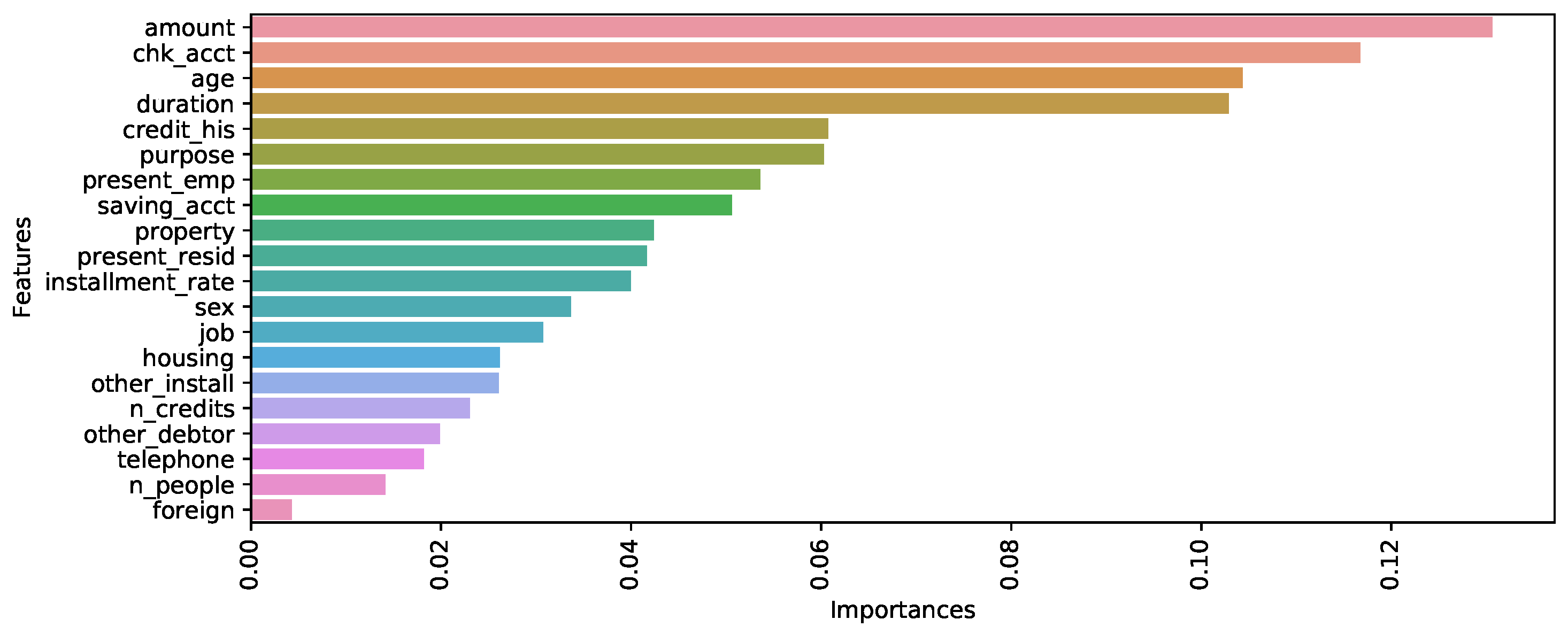
2.3.1. Random Forest Recursive Feature Elimination

Recursive feature elimination (RFE) is a greedy algorithm based on feature-ranking techniques (Zhou et al. 2014). The algorithm measures the classifier performance by eliminating predictors in an iterative manner. In a first step, RFE trains the classifier with all d features, and then it calculates the importance of each feature via the information gain method or the mean reduction in the Gini index (James et al. 2021, p. 336; Ustebay et al. 2018). Subsequently, subsets of progressively smaller sizes $m=d,d-1,\dots ,1$ are created by iterative elimination of the features. The model is retrained within each subset, and its performance is calculated. Hence, RF–RFE is a feature selection method that combines RFE and random forests (see Ustebay et al. 2018 for details). A step-by-step description is given in Algorithm 2.

Algorithm 2 RF–RFE

Train the model in the training set with all d predictors. Compute the overall performance, and rank the predictors by importance. For each subset size m ($m=1,\dots ,d$), repeat the following steps: (a) Train the model by using only the m most important predictors. (b) Compute the classification performance, and rank the m predictors by importance using the mean reduction in Gini index. Use the model based on the optimal number of predictors $m^{*}$, corresponding to the highest performance at Step 3(b) above.

2.3.2. Chi-Squared Feature Selection

In feature selection, we test the null hypothesis of independence by means of the well-known chi-squared test. In particular, we assess whether the class label (the target) is independent of a given feature (Alshaer et al. 2021). The d tests are given by

$${\chi }_s^2=\sum _{i=1}^{m_s}\sum _{j=1}^k\frac{{(O_{ij}-E_{ij})}^2}{E_{ij}},s=1,\dots ,d,$$

where O and E are the observed and expected frequency, respectively, $m_s$ is the number of categories of the sth predictor, and k is the number of classes of the target variable. Continuous features must be discretized.

As usual, large values of ${\chi }_s^2$ imply significant evidence against the null hypothesis of independence of y and $x_s$, and the reference distribution under the null is ${\chi }_{(k-1)(m_s-1)}^2$. Finally, the features $x_s$ for which independence from y cannot be rejected are eliminated from the analysis.

2.3.3. Support Vector Machines and L1-Based Feature Selection

We used support vector machines with linear kernels. The prediction obtained had the general form $\mathrm{pred}\left(\mathit{x}\right)=\mathrm{sign}(b+{\sum }_{i=1}^d{\alpha }_{i}K(\mathit{x},{\mathit{x}}_i))$. If the kernel was linear (i.e., $K(\mathit{x},\mathit{v})={\mathit{x}}^T\mathit{v}$), then the prediction became $\mathrm{sign}(b+{\mathit{w}}^T\mathit{x})$ for $\mathit{w}={(w_1,\dots ,w_d)}^T={({\alpha }_1{x}_1,\dots ,{\alpha }_d{x}_d)}^T$, where $\mathit{w}$ is a vector of weights that can be computed explicitly.

This technique classifies a new observation $(y^{*},{\mathit{x}}^{*})$ by testing whether the linear combination $w_1{x}_1^{*}+\cdots +w_d{x}_d^{*}$ of the components of ${\mathit{x}}^{*}$ is larger or smaller than a given threshold $-b$ (Brankl et al. 2002). Hence, in this approach, the jth feature is more likely to be important if its weight $w_j$ is above the threshold. This type of feature weighting has some intuitive interpretation, because a predictor with a small $|w_j|$ value has a minor impact on the predictions and can be ignored (Sindhwani et al. 2001).

2.4. Over- and Undersampling Techniques

Imbalanced datasets are a relevant issue commonly observed in real-world applications that can have a significant impact on the classification performance of machine learning algorithms. As pointed out by Ganganwar (2012), the available solutions can be grouped into two categories. At the data level, sample-modifying techniques have been developed. At the algorithmic level, cost-sensitive learning methods have been proposed. Here, we apply three algorithms in the former category which have been shown to guarantee a robust solution (Batista et al. 2004). See Baesens et al. (2003) and He and Garcia (2009) for further details.

The basic idea consists of resampling the original dataset, either by oversampling the smallest class or undersampling the largest class until the sizes of the classes are approximately the same. Since undersampling may discard some important information and consequently worsen the performance of the classifiers, oversampling tends to be preferred (Ganganwar 2012).

Random oversampling is one of the simplest methods, as it increases the minority class through randomly repeated copies of the minority class. A possible disadvantage is that if the dataset is large, it may introduce a significant additional computational burden. Moreover, since it yields exact copies of the minority class, it can increase the risk of overfitting.

The synthetic minority oversampling technique (SMOTE; Chawla et al. 2002) oversamples the minority class by synthetically creating new instances rather than oversampling with replacement, as random oversampling does. The SMOTE forms new minority examples by interpolating between several minority class observations that are “close” to each other.

In more detail, given a minority observation ${\mathit{x}}_i$, the K-nearest neighbors of the same class are selected. In a second step, some of these nearest training observations are randomly chosen according to a prespecified oversampling rate. Finally, new synthetic examples are generated along the segment, joining the minority example and its selected nearest neighbors.

SMOTEtomek (Tomek 1976) stands for SMOTE after Tomek and fits into the undersampling group of methods. In this approach, the majority class is undersampled by randomly removing majority class observations until the minority class reaches some specified percentage of the majority class. In particular, the Tomek link discards observations from the most represented class that are close to the least represented class in order to obtain a training dataset with a more clear-cut separation between the two groups.

2.5. Evaluation Criteria

The performance of the models was evaluated based on the established standard measures in the fields of credit scoring. These criteria were the area under the ROC curve (AUC; James et al. 2021, Sect. 4.4.2) and the average accuracy (equal to $1-er$, where er is the error rate). To further strengthen the analysis, we also computed the sensitivity (true positive rate = 1 − Type II error) and the specificity (true negative rate = 1 − Type I error) (see James et al. 2021, p. 152). The basic ingredients are usually represented as follows in the so-called confusion matrix reported in Table 1.

Table 1. Confusion matrix.

		Predicted
		Positive	Negative
Actual	Positive	True positive (TP)	False negative (FN)
	Negative	False positive (FP)	True negative (TN)

Accordingly, the average accuracy, the sensitivity, and the specificity are defined as follows:

$$\mathrm{A}\mathrm{v}.\mathrm{A}\mathrm{c}\mathrm{c}.=\frac{TP+TN}{n},\mathrm{S}\mathrm{e}\mathrm{n}\mathrm{s}.=\frac{TP}{TP+FN},\mathrm{S}\mathrm{p}\mathrm{e}\mathrm{c}.=\frac{TN}{TN+FP}.$$

A default prediction model can misclassify a customer in two ways. First, if the predicted class of a defaulting client is non-default, then the main cost for the bank is the loss of interest and capital. The second error occurs when the model classifies a non-defaulting customer as default and implies the opportunity cost of not lending to a non-defaulting client, which is a missing business opportunity. The cost of the former (i.e., a false negative) is typically higher for a bank.

Several works (see, for example, Dopuch et al. 1987; Koh 1992; Nanda and Pendharkar 2001) suggest that incorporating sensitivity and specificity into the prediction models can lead to more accurate results, especially when the two types of error are associated with different costs. Hence, for decision-making purposes in a banking framework, if a lender can come up with a measure of the cost of the Type I and Type II errors, then proper estimates of sensitivity and specificity can be more important than accuracy.

3. Empirical Analysis

3.1. Dataset Description

The datasets employed for developing credit-scoring models should contain financial characteristics (income, credit history, balance sheet information, …), behavioral information (loan payment behavior, credit usage, …), and categorical variables (age, marital status, …), which are the inputs of the model. In addition, an outcome variable that describes the status of (default or non-default) of the applicant is also known.

In this study, we used a German retail credit dataset downloaded from the UCI machine learning repository1. The dataset refers to the years 1973–1975 and contains 1000 instances and 20 attributes, which give information about the financial statuses of the clients. Of the 20 features, 7 are quantitative and 13 are categorical. To mention just a few of them, we recalled the financial records statuses, measures related to advance rates, bank accounts or securities, installment rates as a percentage of disposable income, and information on the property, age, and number of existing credits. In addition to the 20 features, the dataset contains the target variable credit risk, which is the usual binary variable describing non-creditworthy and creditworthy customers, coded as 1 and 0, respectively. Unfortunately, no information about the definition of default used for constructing the target variable is given. We guessed that the dataset employs the usual definition (i.e., payments missed or delayed by at least 90 days) (see, for example, Duffie and Singleton 2003, p. 44 for possible definitions of the concept). The classes are imbalanced because 300 instances correspond to bad counterparties and 700 instances to good counterparties (Groemping 2019). Table 2 gives the full list.

Table 2. Description of all the features in the German credit dataset.

Column Name	Variable Name	Description
chk acct	Status	Status of the debtor’s checking account with the bank (categorical)
duration	Duration	Credit duration in months (quantitative)
credit his	Credit history	History of compliance with previous or concurrent credit contracts (categorical)
purpose	Purpose	Purpose for which the credit is needed (categorical)
amount	Credit amount	The total amount of credit
saving acct	Saving accounts	Debtor’s savings (categorical)
present emp	Employment duration	Duration of debtor’s employment with current employer (ordinal)
installment rate	Personal status sex	The information about both sex and marital status
sex	Other debtors	If there is another debtor or a guarantor for the credit (categorical)
present resid	Present residence	Length of time (in years) the debtor has lived in the present residence (ordinal)
property	Property	The ranking of debetor’s property in ascending order (ordinal)
age	Age	Age in years (quantitative)
other nstall	Other installment plans	Any credit or installment burden other than the credit given back (categorical)
housing	Housing	Status of current residence (categorical)
n credit	Number credits	The complete history of credit taken (ordinal)
job	Job	The level of debtor’s job (ordinal)
n people	People liable	The total number of peers depending on debtor financially (quantitative)
telephone	Telephone	The status of registered landline on the debtor’s name (binary)
foreign	Foreign worker	If the debtor is a foreign worker (binary)
response	Credit risk	Good or bad (binary)

3.2. Numerical Details

In the empirical analysis, we used five classifiers: neural networks (NNs), naïve Bayes (NB), decision trees (DTs), random forest (RF), K-nearest neighbors, and regularized logistic regression. Three feature selection techniques were employed: chi-squared feature selection, random forest recursive feature elimination, and L1-based feature selection. Since there were fewer defaulters than non-defaulters, the implementation of a preprocessing step to balance the classes was a sensible way of proceeding. We used the SMOTE, SMOTEtomek, and random oversampling algorithms outlined in Section 2.4. However, since the imbalance was not strong, we also performed the analysis with the original imbalanced data.

For the purpose of training and evaluating the models, the dataset was randomly split into a training and a test set in proportions of 75 and 25%, respectively2. The models were implemented in Python with the default parameters using the following packges: Pandas for data manipulation, Matplotlib and Seaborn for data visualization, and Scikit-learn for data preprocessing and fitting the models. For reproducibility purposes, we recall here explicitly the numerical values of the main inputs.

For random forests, the number of trees in the forest was 100. The mean decrease in the Gini index was the measure of the quality of a split in both random forests and decision trees. In the Naïve Bayes approach, the prior probability of each class, ${\pi }_k$ ($k=1,\dots ,M$), was estimated via the relative frequency of the training data in the kth class. As for the univariate distributions of the predictors, they were assumed to be Gaussian in the continuous case, whereas standard nonparametric estimates were used for categorical densities (see, for example, James et al. 2021, p. 156). The KNN algorithm employed a number of neighbors $K=5$3. In neural networks, the activation function for the hidden layer is a rectified linear unit (ReLU). Finally, in regularized logistic regression, the norm of the penalty was ${\ell }_2$4.

3.3. Results

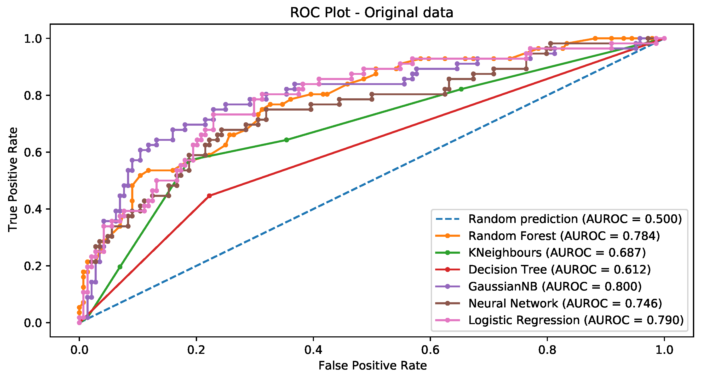
3.3.1. Chi-Squared Feature Selection

Table 3 and Figure 1 display the results obtained with the chi-squared feature selection method of Section 2.3.2. Table 3 lists the seven predictors whose p-values were smaller than 0.01. The actual p-values of the tests are shown in Figure 1. Features corresponding to the test statistics with p-values smaller than 0.01 were considered to be significant for classifying defaulters and non-defaulters.

Table 3. Variables selected via chi-squared feature selection.

Number	Variable	Description
1	Checking accounts	Categorical variable with 4 labels
2	Duration	Numerical variable
3	Credit history	Categorical variable with 5 labels
4	Credit amount	Numerical variable
5	Saving accounts	Categorical variable with 5 labels
6	Present age	Numerical variable
7	Property	Categorical variable with 4 labels

Figure 1. p-values of the chi-squared feature selection procedure.

Table 4 shows the classification performances obtained with the predictors selected via chi-squared feature selection as well as all combinations of the classification algorithms and the sample-modifying approaches used in this paper. For comparison purposes, we reported the outcomes with the original (imbalanced) dataset.

Table 4. Chi-squared feature selection with different classification algorithms. Values in bold are the maximum of each column.

Model	Accuracy	Sensitivity	Specificity	AUC
RF—Imbalanced data	0.746	0.470	0.870	0.755
RF—SMOTE	0.806	0.811	0.800	0.875
RF—SMOTETomek	0.838	0.799	0.878	0.910
RF—RandOverSampling	0.854	0.909	0.800	0.925
DT—imbalanced data	0.680	0.424	0.772	0.598
DT—SMOTE	0.743	0.754	0.731	0.743
DT—SMOTETomek	0.777	0.750	0.805	0.777
DT—RandOverSampling	0.811	0.914	0.709	0.811
GNB—imbalanced data	0.752	0.742	0.755	0.795
GNB—SMOTE	0.691	0.714	0.669	0.736
GNB—SMOTETomek	0.738	0.726	0.750	0.786
GNB—RandOverSampling	0.691	0.663	0.720	0.710
KNN—imbalanced data	0.732	0.439	0.837	0.714
KNN—SMOTE	0.703	0.749	0.657	0.791
KNN—SMOTETomek	0.744	0.756	0.732	0.839
KNN—RandOverSampling	0.680	0.731	0.629	0.771
NN—imbalanced data	0.74	0.5303	0.8152	0.735
NN—SMOTE	0.78	0.789	0.771	0.833
NN—SMOTETomek	0.790	0.811	0.768	0.869
NN—RandOverSampling	0.763	0.771	0.754	0.839
LR—imbalanced data	0.768	0.4848	0.8696	0.782
LR—SMOTE	0.7171	0.7257	0.7086	0.760
LR—SMOTETomek	0.6954	0.6975	0.6933	0.794
LR—RandOverSampling	0.6886	0.6629	0.7143	0.747

We can see that when we employed RF, the model accuracy, sensitivity, specificity, and area under the curve improved significantly with the sample-modifying techniques with respect to the original dataset. Furthermore, when comparing the performance of RF with the different sample-modifying techniques, the combination of random oversampling and random forest achieved the best performance, with an accuracy of 0.854 and $\mathrm{AUC}=0.925$.

As for decision trees, when we used the imbalanced dataset, they had poor performance, being only slightly better than random guessing, with AUC = 0.598 and an accuracy approximately equal to 0.68. In addition, the algorithm tended to favor the most represented class. We conjecture that this was probably caused by the imbalance of the data, since the performance increased significantly by applying sample-modifying techniques. The best combination was based on random oversampling, with an accuracy and AUC equal to 0.8114 and 0.811, respectively.

Turning now to Gaussian Naïve Bayes, we found a rather surprising outcome: when we balanced the data, GNB’s performance decreased with respect to the imbalanced data case. Hence, the best outcome was achieved with imbalanced data. The accuracy of the model was 0.752, and the area under the curve was 0.795, similar to RF with imbalanced data.

Figure 2, Figure 3, Figure 4 and Figure 5 show the ROC curves for the original data (Figure 2) and the data balanced via the SMOTE, SMOTEtomek and random oversampling techniques, respectively (Figure 3, Figure 4 and Figure 5). Each figure displays the ROC curves corresponding to all the classification techniques employed. Overall, the best result was achieved when we combined RF with random oversampling. It is worth noting that all sample-modifying techniques considerably improved the RF algorithm, which was never ranked first when we considered the original imbalanced data but was always clearly the best after balancing the classes.

Figure 2. Imbalanced data.

Figure 3. SMOTE.

Figure 4. SMOTEtomek.

Figure 5. Random oversampling.

The KNN classifier worked rather well by using the imbalanced data, although the most represented class was favored. The best outcome arose from the combination of KNN with the SMOTETomek. In this case, the accuracy was equal to 0.744, and $\mathrm{AUC}=0.839$.

In the neural network case, the performance of the classifier improved significantly with the sample-modifying methods compared with the imbalanced data, and the NN was overall the second-best approach after RF.

Finally, logistic regression performed best when combined with the SMOTETomek. In this case, the AUC was 0.794. However, the performance with imbalanced data was quite similar.

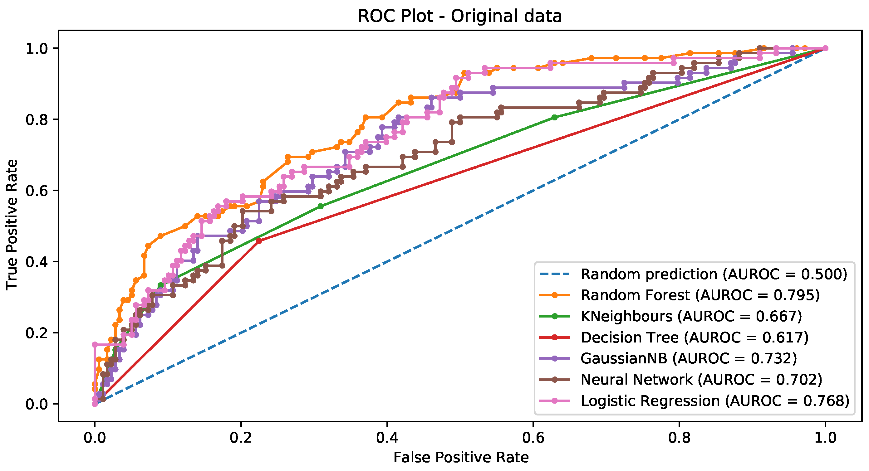
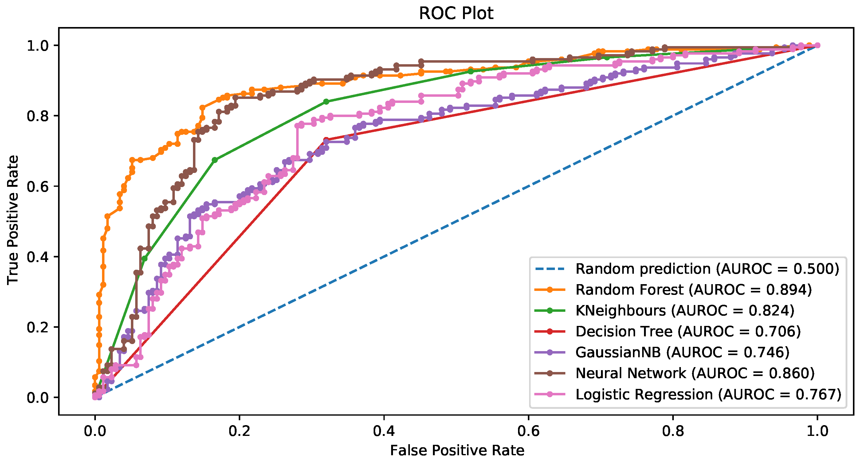
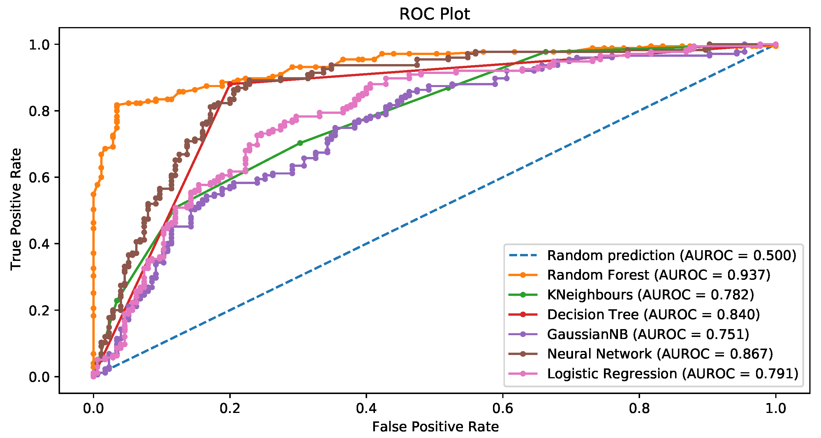
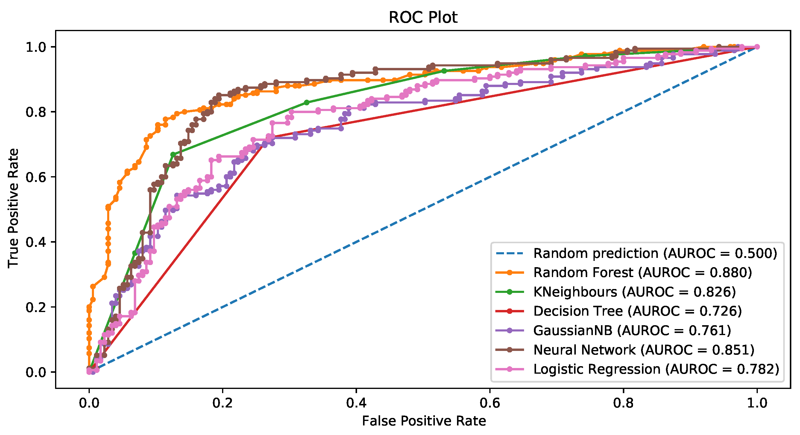
3.3.2. Random Forest Recursive Feature Elimination

When random forest recursive feature elimination was used as a feature selection method, the 10 most important variables according to the mean decrease in the Gini index (James et al. 2021, p. 343) are listed in Table 5. Note that the tenth variable had a mean decrease equal to 0.042. With only one exception (present age), the 7 features selected by Chi-squared feature selection were a subset of the 10 predictors chosen via random forest recursive feature elimination. This suggests that the selection of the relevant predictors was rather robust with respect to the algorithm employed for this goal.

Table 5. The 10 most important predictors obtained via random forest recursive feature elimination.

Number	Variable	Description
1	Credit amount	Numerical variable
2	Checking accounts	Categorical variable with 4 labels
3	Age	Numerical variable
4	Duration	Numerical variable
5	Credit history	Categorical variable with 5 labels
6	Purpose	Categorical variable with 4 labels
7	Present employment since	Categorical variable with 5 labels
8	Savings account	Categorical variable with 5 labels
9	Property	Categorical variable with 4 labels
10	Present residence	Numerical variable

Figure 6 shows the importance of all variables, as measured by the mean decrease in the Gini index.

Figure 6. The importance of the variables in the random forest recursive feature elimination approach. Importance was measured via the mean decrease in the Gini index.

Table 6 reports the results obtained when we used different sample-modifying techniques with the features selected by random forest recursive elimination.

Table 6. Random forest recursive feature elimination with different classification algorithms. Values in bold are the maximum of each column.

Model	Accuracy	Sensitivity	Specificity	AUC
RF—imbalanced data	0.788	0.444	0.927	0.795
RF—SMOTE	0.823	0.794	0.851	0.894
RF—SMOTETomek	0.823	0.846	0.800	0.895
RF—RandOverSampling	0.843	0.869	0.817	0.932
DT—imbalanced data	0.684	0.458	0.775	0.617
DT—SMOTE	0.706	0.731	0.680	0.706
DT—SMOTETomek	0.7200	0.751	0.688	0.720
DT—RandOverSampling	0.831	0.903	0.760	0.831
GNB—imbalanced data	0.708	0.486	0.798	0.732
GNB—SMOTE	0.694	0.703	0.686	0.746
GNB—SMOTETomek	0.696	0.722	0.671	0.749
GNB—RandOverSampling	0.654	0.577	0.731	0.717
KNN—imbalanced data	0.744	0.333	0.910	0.667
KNN—SMOTE	0.760	0.840	0.680	0.824
KNN—SMOTETomek	0.699	0.846	0.553	0.789
KNN—RandOverSampling	0.706	0.714	0.697	0.771
NN—imbalanced data	0.712	0.431	0.826	0.702
NN—SMOTE	0.823	0.840	0.806	0.860
NN—SMOTETomek	0.796	0.882	0.712	0.865
NN—RandOverSampling	0.803	0.806	0.800	0.863
LR—imbalanced data	0.752	0.4306	0.882	0.768
LR—SMOTE	0.7086	0.6971	0.72	0.767
LR—SMOTETomek	0.7351	0.7337	0.6964	0.809
LR—RandOverSampling	0.74	0.7543	0.7257	0.791

Both RF and DT performed better with random oversampling than with the other sample-modifying techniques. It is worth noting that RF with random oversampling was characterized by the highest accuracy and AUC among all methods, whereas DT had the largest specificity. These results were quite similar to those achieved when using the chi-squared feature selection algorithm.

Gaussian Naïve Bayes obtained comparable results with the different sample-modifying techniques, but the outcomes were worse than those based on the imbalanced data. KNN performed well with the SMOTE compared with the other techniques, with 0.76 accuracy and an AUC of 0.824. The neural network’s performance was similar with all the sample-modifying techniques and better with respect to the performance with the imbalanced data. Finally, the performance of the logistic regression was not significantly enhanced by the sample-modifying techniques, whose outcomes were more or less comparable.

To sum up, in this case, for most classifiers, the performance as measured by the AUC also significantly improved compared with the models based on imbalanced data. Similar to Section 3.3.1, however, sample-modifying did not help when combined with GNB, where the best outcomes were obtained with the original data, and with LR, where the AUC remained approximately the same with and without sample-modifying techniques. Overall, the best performance was given by random forests with random oversampling, with an AUC and accuracy of 0.932 and 0.8429, respectively. The largest specificity (0.927) was obtained by RF with imbalanced data at the price of a very low sensitivity (0.444). As for sensitivity, DT with random oversampling achieved the largest value, but its AUC was smaller than that for RF with random oversampling.

All in all, the results yielded by random forest recursive feature elimination were similar to those obtained by chi-squared feature selection (see Table 4). Since, as noted above, the predictors selected by chi-squared selection and random forest recursive feature elimination were quite similar, this is not a suprising outcome.

Figure 7, Figure 8, Figure 9 and Figure 10 show the ROC curves for the original data (Figure 7) and the data balanced via the SMOTE, SMOTEtomek, and random oversampling, respectively (Figure 8, Figure 9 and Figure 10). Each figure displays the ROC curves corresponding to all the classification techniques employed.

Figure 7. Imbalanced data.

Figure 8. SMOTE.

Figure 9. SMOTEtomek.

Figure 10. Oversampling.

The plots are again similar to the results in Section 3.3.1. We observe that the highest AUC resulted from the use of random forests and random oversampling. Moreover, sample modifying was especially beneficial for the RF classifier, and GNB was the only case where sample-modifying methods mostly decreased the predictive accuracy.

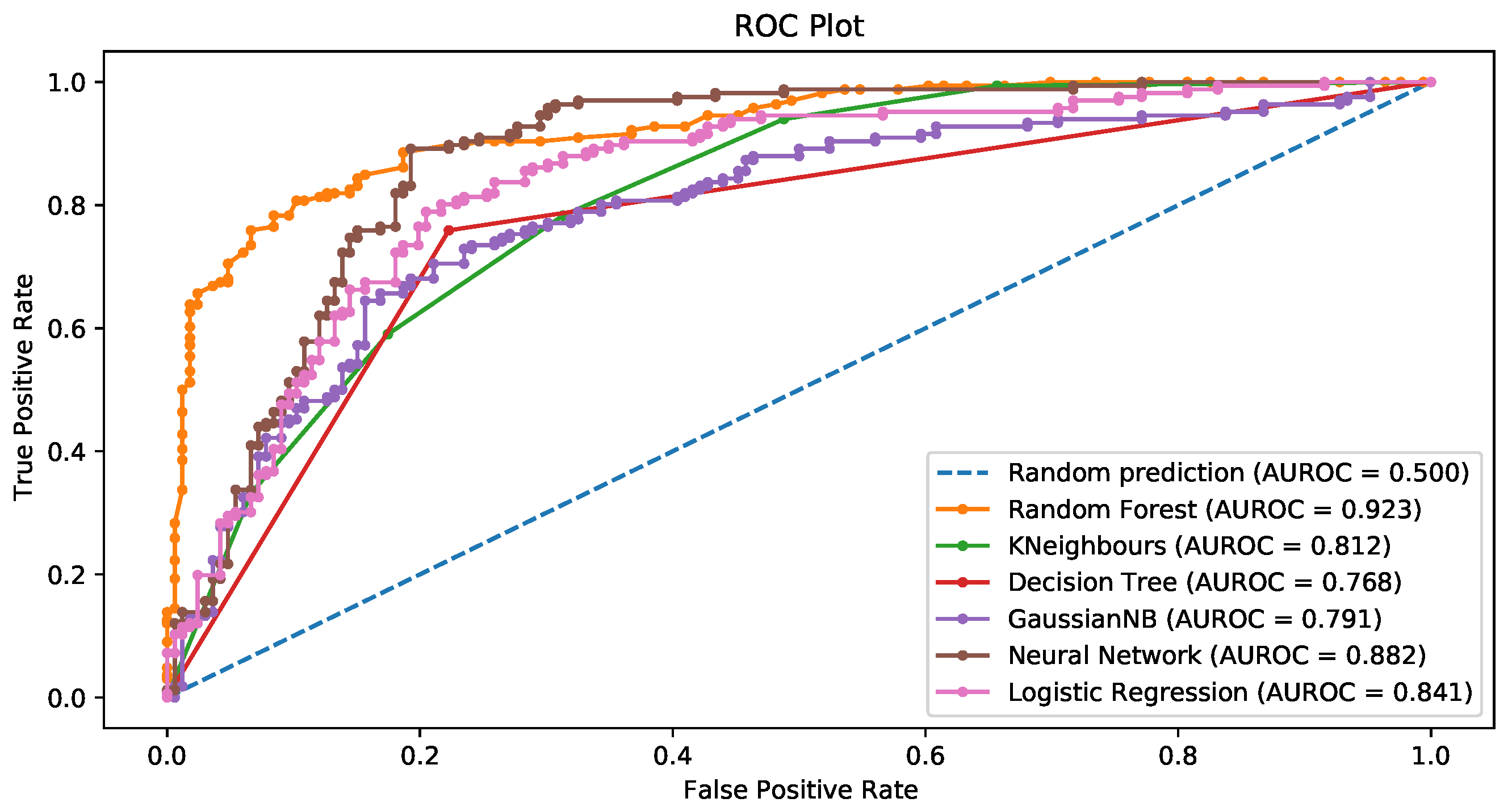
3.3.3. L1-Based Feature Selection

The last feature selection approach employed in this paper is the L1-based criterion introduced in Section 2.3.3. Recall that in this algorithm, the features associated to coefficients not equal to zero are considered to contribute significantly to the prediction of the target variable. Table 7 lists the nine best default predictors according to the L1-based algorithm.

Table 7. The nine best predictors obtained via L1-based feature selection.

Number	Variable	Description
1	Checking accounts	Categorical variable with 4 labels
2	Duration	Numerical variable
3	Credit history	Categorical variable with 5 labels
4	Age	Numerical variable
5	Credit amount	Numerical variable
6	Saving account	Categorical variable with 5 labels
7	Present employment since	Categorical variable with 5 labels
8	Present Instalment rate	Numerical variable
9	Property	Categorical variable with 4 labels

Table 8 confirms the results obtained in Section 3.3.1 and Section 3.3.2: the random forest classifier with random oversampling had the best performance, with an accuracy equal to 0.8571 and $\mathrm{AUC}=0.925$. However, random forest also performed well with the SMOTE and SMOTETomek. Analogously, the decision trees performed best when combined with random oversampling.

Table 8. L1-based feature selection with different classification algorithms. Values in bold are the maximum of each column.

Model	Accuracy	Sensitivity	Specificity	AUC
RF—imbalanced data	0.765	0.393	0.910	0.784
RF—SMOTE	0.820	0.811	0.829	0.880
RF—SMOTETomek	0.812	0.844	0.780	0.922
RF—RandOverSampling	0.857	0.903	0.811	0.920
DT—imbalanced data	0.685	0.446	0.778	0.612
DT—SMOTE	0.726	0.720	0.731	0.726
DT—SMOTETomek	0.749	0.790	0.708	0.749
DT—RandOverSampling	0.840	0.886	0.794	0.840
GNB—imbalanced data	0.765	0.750	0.771	0.800
GNB—SMOTE	0.700	0.731	0.669	0.761
GNB—SMOTETomek	0.758	0.844	0.673	0.803
GNB—RandOverSampling	0.657	0.623	0.691	0.743
KNN—imbalanced data	0.745	0.571	0.812	0.687
KNN—SMOTE	0.751	0.829	0.674	0.826
KNN—SMOTETomek	0.773	0.922	0.625	0.856
KNN—RandOverSampling	0.706	0.709	0.703	0.772
NN—imbalanced data	0.735	0.446	0.847	0.746
NN—SMOTE	0.829	0.851	0.806	0.851
NN—SMOTETomek	0.797	0.838	0.756	0.861
NN—RandOverSampling	0.791	0.771	0.811	0.848
LR—imbalanced data	0.755	0.4286	0.8819	0.790
LR—SMOTE	0.7314	0.7086	0.7543	0.782
LR—SMOTETomek	0.7861	0.8072	0.7651	0.841
LR—RandOverSampling	0.6857	0.6343	0.7371	0.741

Additionally, in this case, Gaussian Naïve Bayes had comparable behavior with the three sample-modifying techniques but tended to achieve better outcomes with the original (imbalanced) data. KNN had overall good performance, and in particular yields, when combined with the SMOTETomek, it had the highest sensitivity among all the classifiers considered in Table 8.

Neural networks gave the best results with the SMOTE, with an accuracy and AUC equal to 0.8286 and 0.851, respectively. It was the second best-performing model after random forests. Finally, logistic regression yielded good outcomes. It is worth noting that in this case, the SMOTEtomek yielded the largest improvement, especially concerning sensitivity and AUC.

Figure 11, Figure 12, Figure 13 and Figure 14 show the ROC curves for the original data (Figure 11) and the data balanced via the SMOTE, SMOTEtomek, and random oversampling, respectively (Figure 12, Figure 13 and Figure 14). Each plot displays the ROC curves corresponding to all the classification techniques employed.

Figure 11. Imbalanced data.

Figure 12. SMOTE.

Figure 13. SMOTEtomek.

Figure 14. Random oversampling.

Similar to the cases of the two feature selection methods analyzed in the previous two sections, the most striking feature of the plots is the strong improvement of RF when combined with sample-modifying techniques.

3.3.4. Computational Efficiency

Table 9 summarizes the training computing times. We have only reported the results with random oversampling, since the SMOTE and SMOTEtomek techniques are very similar. We can see that Naïve Bayes had the lowest training time, while the algorithm with the highest training time was the neural network.

Table 9. Running time of the algorithms (in seconds).

Model	ChiSquare	RF-RFE	L1
RF—RandOverSampling	0.6088	0.4214	0.2902
DT—RandOverSampling	0.0089	0.0109	0.0089
GNB—RandOverSampling	0.0079	0.0059	0.0079
KNN—RandOverSampling	0.0448	0.0468	0.0408
NN—RandOverSampling	1.8018	1.5998	1.8516
LR—RandOverSampling	0.0279	0.0259	0.0229

These outcomes are not surprising, since it is well known that Naïve Bayes is an approach that often trades some predictive power with computational efficiency, whereas neural networks are a complex method whose estimation is more time-consuming. In this set-up, all computing times are rather small, so the practical implementation of all the algorithms should not be difficult, even in larger datasets with more predictors.

3.3.5. General Comments about the Results

The main message of the analysis run in the preceding sections is that random forest was the best classifier in terms of average accuracy and AUC, and artificial neural networks also showed good performance with respect to the other ML algorithms. It is worth stressing that a traditional statistical approach such as logistic regression also worked quite well. This outcome suggests that statistical techniques are still effective and reliable tools for credit scoring. Given that LR is also highly interpretable and already well known by banks and practitioners, it may be convenient for banks to use both approaches (statistical and ML-based) when routinely predicting customer defaults in daily business practices.

All the feature-selection algorithms yielded very similar sets of predictors. Not surprisingly, this implies that, with any of them, one would obtain similar classification outcomes. If we look at the sample-modifying techniques, in the best classification approach (i.e., random forest), random oversampling was preferable to the SMOTE and SMOTEtomek techniques in terms of both accuracy and AUC. However, the SMOTE or SMOTEtomek techniques were sometimes better when we considered other classification algorithms. Overall, the best method was random forest combined with random oversampling.

The performance of almost all classifiers improved significantly with the sample-modifying techniques, with respect to the base imbalanced data case. The only exception was the Naïve Bayes algorithm, which also had comparable performance when the data were imbalanced. Another general result is that sample-modifying techniques are especially beneficial in terms of sensitivity.

Tree-based techniques (i.e., decision trees and random forests) had higher performance when combined with random oversampling. Moreover, they gained more than other classifiers from the use of sample-modifying methods. According to our results, the best combination of algorithms to build a robust, accurate, and sensitive credit-scoring model is random forest combined with random forest recursive feature elimination and the random oversampling technique.

The dataset employed in this section has already been used in ML applications in the past (see, for example, Dea et al. (2001); Ekin et al. (1999); Gonzalez et al. (2001); Ustebay et al. (2018); Wang et al. (2003)). However, Ustebay et al. (2018) performed unsupervised learning analysis, whereas Wang et al. (2003) studied the impact of modifications of the dataset, so these two studies are not directly comparable to our work. The other three articles employed selection and learning techniques that were different from ours, but some comparison is sensible. Dea et al. (2001) used a neural network-like algorithm. They selected seven features, analogous to what we obtained in Table 3, and most features were the same in both cases. The accuracy in the test set was 74.25%, essentially equal to what we showed in Table 4. Similar accuracies were also obtained by Ekin et al. (1999) via distance-based methods. Gonzalez et al. (2001) developed a graph-based relational concept learner. In this case, the highest accuracy was 71.52%.

Our results suggest that ML techniques are a powerful tool for credit scoring and default prediction purposes. From the economic point of view, inaccurate estimates of creditworthiness in the banking sector were the key determinant of the two worst economic crises of modern times (i.e., the Great Depression of 1929 and the Great Recession of 2008). The latter in particular was triggered by the so-called subprime mortgage crisis, where underestimation of default probabilities and easy credit conditions had catastrophic economic consequences. The use of ML approaches such as the ones proposed in the current paper, possibly combined with more traditional statistical techniques and under strict regulatory control, is an additional shelter against further crises.

3.3.6. Dealing with a More-Imbalanced Set-Up

In the preceding section, we studied the performance of the classifiers and the data-balancing techniques in a framework where classes were moderately imbalanced. Since typical credit datasets are more imbalanced5, one may wonder whether the results obtained in Section 3.3 can be generalized to a more imbalanced set-up.

To investigate this issue, in this section, we perform the same analysis in an extremely imbalanced dataset. Specifically, we used the Default dataset from the ISLR R package, which contains 10,000 simulated credit card default observations, consisting of a target variable (default indicator) and three features with a percentage of defaults equal to 3.33%. For simplicity, we only implemented random forests, neural networks, and logistic regression, since these approaches turned out to be very effective in the German credit dataset. Table 10 illustrates the performance of the classifiers with different data-balancing techniques.

Table 10. Performance of RF, NN, and LR in the Default dataset. Values in bold are the maximum of each column.

Model	Accuracy	Sensitivity	Specificity	AUC
RF—Imbalanced	0.9690	0.3889	0.9909	0.8526
RF—SMOTE	0.9200	0.8858	0.9371	0.9664
RF—SMOTETomek	0.9498	0.9384	0.9552	0.9812
RF—RandOverSampling	0.9846	1.000	0.9768	0.9998
NN—Imbalanced	0.9724	0.3333	0.9963	0.9445
NN—SMOTE	0.8756	0.8113	0.9077	0.9511
NN—SMOTETomek	0.9070	0.8524	0.9335	0.9654
NN—RandOverSampling	0.8745	0.8311	0.8962	0.9493
LR—Imbalanced	0.9724	0.3222	0.9967	0.9465
LR—SMOTE	0.8748	0.8022	0.9110	0.9493
LR—SMOTETomek	0.9027	0.8339	0.9361	0.9650
LR—RandOverSampling	0.8737	0.8055	0.9077	0.9479

From Table 10, we see that RF combined with random oversampling had the best performance in terms of accuracy ($0.9846$) and AUC ($0.9998$), which is in line with the outcomes obtained in Section 3.3. The use of data-balancing techniques yielded mixed results. On one hand, all methods significantly improved the sensitivity, similar to the German credit dataset. In terms of accuracy, the results were worse for the NN and LR and remained approximately the same for RF. The AUC was improved for RF and not significantly different for the NN and RF. As in the German credit dataset, RF was the classifier that gained more from the combination with data-balancing techniques, especially with random oversampling.

4. Conclusions

Recently, many studies have shed light on credit scoring, which has become one of the cornerstones of credit risk measurement. In this paper, we tried to identify the most important predictors of credit default for the purpose of constructing machine learning classifiers that identify defaulters and non-defaulters as efficiently as possible.

Since our data were imbalanced, we implemented three sample-modifying algorithms and subsequently assessed the performance improvement of the classification models. The take-home messages are that random forest combined with any feature selection algorithm and with random oversampling is the best classifier, and data-balancing algorithms are beneficial, especially for improving sensitivity.

In terms of classifier performance, similar outcomes were obtained by De Castro Vieira et al. (2019) and Trivedi (2020). Given that, in recent years, there has been an exponentially increasing number of papers employing machine learning for the construction of credit scoring, it is difficult to give a detailed list of the results in the literature here. A good starting point is the references in Leo et al. (2019, sct. 3.1).

A possible limitation of this study is that a moderately large dataset was used in the main application. The second empirical analysis was based on a larger sample and seemed to confirm the results, but the data were simulated. Hence, the use of a larger real dataset should be considered to double-check the accuracy of the models. Another issue open to further research is the use of different credit categories to test the models. In future research, we plan to extend the investigation to corporate defaults. Finally, the impact of sample-modifying techniques in datasets where classes are more imbalanced is also worth further scrutiny.

References

- Alshaer, Hadeel N., Mohammed A. Otair, Laith Abualigah, Mohammad Alshinwan, and Ahmad M. Khasawneh. 2021. Feature selection method using improved Chi Square on Arabic text classifiers: Analysis and application. Multimedia Tools and Applications 80: 10373–90. [Google Scholar] [CrossRef]
- Anderson, Raymond. 2007. The Credit Scoring Toolkit—Theory and Practice for Retail Credit Risk Management and Decision Automation. Oxford: Oxford University Press. [Google Scholar]
- Baesens, Bart, T. Van Gestel, S. Viaene, M. Stepanova, J. Suykens, and J. Vanthienen. 2003. Benchmarking state-of-the-art classification algorithms for credit scoring. Journal of the Operational Research Society 54: 627–35. [Google Scholar] [CrossRef]
- Batista, Gustavo E. A. P. A., Ronaldo C. Prati, and Maria Carolina Monard. 2004. A study of the behavior of several methods for balancing machine learning training data. ACM SIGKDD Explorations Newsletter 6: 20–29. [Google Scholar] [CrossRef]
- Bolder, David Jamieson. 2018. Credit-Risk Modelling: Theoretical Foundations, Diagnostic Tools, Practical Examples, and Numerical Recipes in Python. New York: Springer. [Google Scholar]
- Brankl, Janez, M. Grobelnikl, N. Milić-Frayling, and D. Mladenić. 2002. Feature selection using support vector machines. In Data Mining III. Edited by A. Zanasi, C. Brebbia, N. Ebecken and P. Melli. Southampton: WIT Press. [Google Scholar]
- Breiman, Leo. 2001. Random forests. Machine Learning 45: 5–32. [Google Scholar] [CrossRef] [Green Version]
- Breiman, Leo, Jerome H. Friedman, Charles J. Stone, and Richard A. Olshen. 1984. Classification and Regression Trees. London: Chapman and Hall. [Google Scholar]
- Buta, Paul. 1994. Mining for financial knowledge with CBR. AI Expert 9: 34–41. [Google Scholar]
- Chandrashekar, Girish, and Ferat Sahin. 2014. A survey on feature selection methods. Computers & Electrical Engineering 40: 16–28. [Google Scholar]
- Chawla, Nitesh V., Kevin W. Bowyer, Lawrence O. Hall, and W. Philip Kegelmeyer. 2002. Smote: Synthetic minority over-sampling technique. Journal of Artificial Intelligence Research 16: 321–57. [Google Scholar] [CrossRef]
- Chen, Mu-Chen, and Shih-Hsien Huang. 2003. Credit scoring and rejected instances reassigning through evolutionary computation techniques. Expert Systems with Applications 24: 433–41. [Google Scholar] [CrossRef]
- De Castro Vieira, José Rômulo, Flavio Barboza, Vinicius Amorim Sobreiro, and Herbert Kimura. 2019. Machine learning models for credit analysis improvements: Predicting low-income families’ default. Applied Soft Computing 83: 105640. [Google Scholar] [CrossRef]
- Dea, Paul O., Josephine Griffith, and Colm O. Riordan. 2001. Combining feature selection and neural networks for solving classification problems. Paper presented at the 12th Irish Conference on Artificial Intelligence and Cognitive Science, Dublin, Ireland, December 9–10. [Google Scholar]
- Denison, David G. T., Christopher C. Holmes, Bani K. Mallick, and Adrian F. M. Smith. 2002. Bayesian Methods for Nonlinear Classification and Regression. Hoboken: John Wiley & Sons, vol. 386. [Google Scholar]
- Desai, Vijay S., Jonathan N. Crook, and George A. Overstreet Jr. 1996. A comparison of neural networks and linear scoring models in the credit union environment. European Journal of Operational Research 95: 24–37. [Google Scholar] [CrossRef]
- Dopuch, Nicholas, Robert W. Holthausen, and Richard W. Leftwich. 1987. Predicting audit qualifications with financial and market variables. Accounting Review 62: 431–454. [Google Scholar]
- Duffie, Darrell, and Kenneth J. Singleton. 2003. Credit Risk: Pricing, Measurement, and Management. Princeton: Princeton University Press. [Google Scholar]
- Ekin, Oya, Peter L. Hammer, Alexander Kogan, and Pawel Winter. 1999. Distance-based classification methods. INFOR: Information Systems and Operational Research 37: 337–52. [Google Scholar] [CrossRef]
- Friedman, Jerome H. 1991. Multivariate adaptive regression splines. The Annals of Statistics 19: 1–67. [Google Scholar] [CrossRef]
- Ganganwar, Vaishali. 2012. An overview of classification algorithms for imbalanced datasets. International Journal of Emerging Technology and Advanced Engineering 2: 42–47. [Google Scholar]
- Gonzalez, Jesus A., Lawrence B. Holder, and Diane J. Cook. 2001. Graph-based concept learning. In Proceedings of the Florida Artificial Intelligence Research Symposium. Palo Alto: AAAI/IAAI. [Google Scholar]
- Groemping, Ulrike. 2019. South German credit data: Correcting a widely used data set. Reports in Mathematics, Physics and Chemistry, Berichte aus der Mathematik, Physik und Chemie 4: 2019. [Google Scholar]
- Hand, David J., and William E. Henley. 1997. Statistical classification methods in consumer credit scoring: A review. Journal of the Royal Statistical Society: Series A 160: 523–41. [Google Scholar] [CrossRef]
- Haykin, Simon S. Neural Networks: A Comprehensive Foundation, 2nd ed. Upper Saddle River: Prentice Hall PTR.
- He, Haibo, and Edwardo A. Garcia. 2009. Learning from imbalanced data. IEEE Transactions on Knowledge and Data Engineering 21: 1263–84. [Google Scholar]
- Huang, Cheng-Lung, Mu-Chen Chen, and Chieh-Jen Wang. 2007. Credit scoring with a data mining approach based on support vector machines. Expert Systems with Applications 33: 847–56. [Google Scholar] [CrossRef]
- Huang, Zan, Hsinchun Chen, Chia-Jung Hsu, Wun-Hwa Chen, and Soushan Wu. 2004. Credit rating analysis with support vector machines and neural networks: A market comparative study. Decision Support Systems 37: 543–58. [Google Scholar] [CrossRef]
- Hung, Chihli, and Jing-Hong Chen. 2009. A selective ensemble based on expected probabilities for bankruptcy prediction. Expert Systems with Applications 36: 5297–303. [Google Scholar] [CrossRef]
- James, Gareth, Daniela Witten, Trevor Hastie, and Rob Tibshirani. 2021. An Introduction to Statistical Learning, 2nd ed. New York: Springer. [Google Scholar]
- Karels, Gordon V., and Arun J. Prakash. 1987. Multivariate normality and forecasting of business bankruptcy. Journal of Business Finance & Accounting 14: 573–93. [Google Scholar]
- Koh, Hian Chye. 1992. The sensitivity of optimal cutoff points to misclassification costs of type I and type II errors in the going-concern prediction context. Journal of Business Finance & Accounting 19: 187–97. [Google Scholar]
- Leo, Martin, Suneel Sharma, and Koilakuntla Maddulety. 2019. Machine learning in banking risk management: A literature review. Risks 7: 29. [Google Scholar] [CrossRef] [Green Version]
- Makowski, Paul. 1985. Credit scoring branches out. Credit World 75: 30–37. [Google Scholar]
- Moscatelli, Mirko, Simone Narizzano, Fabio Parlapiano, and Gianluca Viggiano. 2020. Corporate default forecasting with machine learning. Expert Systems with Applications 161: 113567. [Google Scholar] [CrossRef]
- Nanda, Sudhir, and Parag Pendharkar. 2001. Linear models for minimizing misclassification costs in bankruptcy prediction. Intelligent Systems in Accounting, Finance & Management 10: 155–68. [Google Scholar]
- Reichert, Alan K., Chien-Ching Cho, and George M. Wagner. 1983. An examination of the conceptual issues involved in developing credit-scoring models. Journal of Business & Economic Statistics 1: 101–14. [Google Scholar]
- Schebesch, Klaus Bruno, and Ralf Stecking. 2005. Support vector machines for classifying and describing credit applicants: Detecting typical and critical regions. Journal of the Operational Research Society 56: 1082–88. [Google Scholar] [CrossRef]
- Shin, Kyung-shik, and Ingoo Han. 2001. A case-based approach using inductive indexing for corporate bond rating. Decision Support Systems 32: 41–52. [Google Scholar] [CrossRef]
- Sindhwani, Vikas, Pushpak Bhattacharya, and Subrata Rakshit. 2001. Information theoretic feature crediting in multiclass support vector machines. In Proceedings of the 2001 SIAM International Conference on Data Mining. Philadelphia: SIAM, pp. 1–18. [Google Scholar]
- Thomas, Lyn C. 2000. A survey of credit and behavioural scoring: Forecasting financial risk of lending to consumers. International Journal of Forecasting 16: 149–72. [Google Scholar] [CrossRef]
- Tomek, Ivan. 1976. Two modifications of cnn. IEEE Transactions on Systems, Man, and Cybernetics 11: 769–72. [Google Scholar]
- Trivedi, Shrawan Kumar. 2020. A study on credit scoring modeling with different feature selection and machine learning approaches. Technology in Society 63: 101413. [Google Scholar] [CrossRef]
- Tsai, Chih-Fong, and Ming-Lun Chen. 2010. Credit rating by hybrid machine learning techniques. Applied Soft Computing 10: 374–80. [Google Scholar] [CrossRef]
- Ustebay, Serpil, Zeynep Turgut, and Muhammed Ali Aydin. 2018. Intrusion detection system with recursive feature elimination by using random forest and deep learning classifier. Paper presented at the 2018 International Congress on Big Data, Deep Learning and Fighting Cyber Terrorism (IBIGDELFT), Ankara, Turkey, December 3–4; pp. 71–76. [Google Scholar]
- Van Gestel, Tony, and Bart Baesens. 2009. Credit Risk Management. Basic Concepts: Financial Risk Components, Rating Analysis, Models, Economic and Regulatory Capital. Oxford: Oxford University Press. [Google Scholar]
- Wang, Gang, Jinxing Hao, Jian Ma, and Hongbing Jiang. 2011. A comparative assessment of ensemble learning for credit scoring. Expert Systems with Applications 38: 223–30. [Google Scholar] [CrossRef]
- Wang, Ke, Senqiang Zhou, Ada Wai-Chee Fu, and Jeffrey Xu Yu. 2003. Mining changes of classification by correspondence tracing. Paper presented at the 2003 SIAM International Conference on Data Mining (SDM), San Francisco, CA, USA, May 1–3. [Google Scholar]
- West, David. 2000. Neural network credit scoring models. Computers & Operations Research 27: 1131–52. [Google Scholar]
- Yu, Lean, Shouyang Wang, and Kin Keung Lai. 2008. Credit risk assessment with a multistage neural network ensemble learning approach. Expert Systems with Applications 34: 1434–44. [Google Scholar] [CrossRef]
- Zhou, Qifeng, Hao Zhou, Qingqing Zhou, Fan Yang, and Linkai Luo. 2014. Structure damage detection based on random forest recursive feature elimination. Mechanical Systems and Signal Processing 46: 82–90. [Google Scholar] [CrossRef]
Publisher’s Note: MDPI stays neutral with regard to jurisdictional claims in published maps and institutional affiliations. |
© 2022 by the authors. Licensee MDPI, Basel, Switzerland. This article is an open access article distributed under the terms and conditions of the Creative Commons Attribution (CC BY) license (https://creativecommons.org/licenses/by/4.0/).