Article

Measurement of Systemic Risk in the Colombian Banking Sector

by
Orlando Rivera-Escobar
1,
John Willmer Escobar
2,* and
Diego Fernando Manotas
3
1
Department of Economic Sciences, Universidad del Valle, Cali 760001, Colombia
2
Department of Accounting and Finance, Universidad del Valle, Cali 760001, Colombia
3
School of Industrial Engineering, Universidad del Valle, Cali 760001, Colombia
*
Author to whom correspondence should be addressed.
Risks 2022, 10(1), 22; https://doi.org/10.3390/risks10010022
Submission received: 26 October 2021 / Revised: 30 November 2021 / Accepted: 2 December 2021 / Published: 13 January 2022
(This article belongs to the Special Issue Data Analysis for Risk Management – Economics, Finance and Business)

Abstract

:
This paper uses three methodologies for measuring the existence of systemic risk in the Colombian banking system. The determination of its existence is based on implementing three systemic risk measures widely referenced in academic works after the subprime crisis, known as CoVaR, MES and SRISK. Together, the three methodologies were implemented for the case of Colombian Banks during the 2008–2017 period. The findings allow us to establish that the Colombian banking sector did not present a systemic risk scenario, despite having suffered economic losses due to external shocks, mainly due to the subprime crisis. The results and findings show the efficiency of the systemic risk measures implemented in this study as an alternative to measure systemic risk in banking systems.

1. Introduction

After the financial crisis of 2007–2008, the debate on the systemic risk that materialized took center stage. This circumstance led both the financial regulatory institutions and the academy to take part in the different debates generated to know, in a better way, the circumstances and facts that would have provided the necessary inputs for the realization and materialization of this type of risk.
The results of this crisis produced severe consequences and high costs for the economy and society. Although many of the costs involved in the development and subsequent outcome are not directly quantifiable, it is estimated that banks’ costs would be around 2.3 trillion dollars (International Monetary Fund 2010). On the other hand, both direct and indirect impacts on the real sector materialized in economic losses and weakened confidence in the markets and the economy. These events provided the necessary inputs for the appearance of major adverse events such as deflation and economic stagnation (Cáceres 2009). The above results made systemic risk one of the central research topics, thus generating many contributions encouraged by providing answers to the questions generated during and after the subprime crisis.
Within the expected results of the various contributions made to the debate on systemic risk, there is a tendency to suggest that a determining factor would be integration between markets. Over time, financial crises have tended to broaden and deepen more and more, to the extent that the financial sector’s participation within economies has increased significantly. This increase goes hand in hand with technological advances in the computing and information sectors, which, together with other factors, have consolidated a continuous and solid integration between global and local financial markets (Guerra et al. 2016; Silva et al. 2017). In this way, the above events would support the necessary mechanisms for the spread and accentuation of systemic risk events between economies and within them, regardless of their growth and development levels (Grilli et al. 2015).
On the other hand, the financial sector’s participation within economies would be a key factor when evaluating the impacts and spread. The financial crisis of 2008, from now on subprime crisis, also evidenced that the inefficient participation of financial regulation and the prevalence of moral hazard in decision-making by credit institutions and risk evaluators contributed to the creation and extension of systemic risk, which as a result produced the bankruptcy of the largest banks and mortgage institutions in the United States and Europe during 2008 (Cáceres 2009).
The subprime crisis caused an indecision environment due to the lack of consensus regarding its definition and measure. The systemic risk concept had already been addressed in studies before the subprime crisis; however, these did not represent a point of collective interest, and thus remained underdeveloped (Drakos and Kouretas 2015; Silva et al. 2017). As a result of the previous, more information and consensus regarding its consequences than its causes has been fostered (Guerra et al. 2016).
For this article’s purpose, the definition of systemic risk proposed in the Report on Financial Consolidation for the year 2001 proposed by the Bank for International Settlements BIS is used. Systemic risk is defined as the risk induced by exogenous shocks that trigger losses in the economic value of a significant portion of the financial system, and with these, the imposition of adverse effects on the real economy. Based on the findings, the definition proposed here adequately captures the Colombian economy’s role during the subprime crisis. However, the economic losses experienced by the banking sector were not significant enough to materialize in a scenario of systemic crisis. Furthermore, the negative impact imposed on the real sector by the banking sector was carried out mainly through the restriction of the supply of credit by them, as a measure to limit their exposure to credit risk (Cáceres 2009).
The vulnerability of financial systems, both national and international, to a possible realization of a new systemic crisis has been a latent concern due to the lack of dynamism on the part of regulatory policies; despite showing the dynamics present in the financial systems, they remained static without corresponding to these dynamics. This idea is commonly found in the works carried out by Drakos and Kouretas (2015); López-Espinosa et al. (2012) and Castelao et al. (2013), among others. By the above, it is necessary to implement strategies or policies to neutralize or reduce the transmission mechanisms by which systemic risk empowers the system’s stability. In this way, this paper proposes a methodology for measuring systemic risk based on using three risk measures that capture each banking institution’s contribution to global risk. Likewise, the identification of the characteristics conducive to systemic risk in banking entities is determined. In this way, it is possible to evaluate the incidence and the individualization of the determining factors for the generation of systemic risk in the Colombian banking system.
The proposed methodology is based on the implementation of various systemic risk measures. The choice to use different measures to contribute to systemic risk is based on the difficulty of capturing the multiple facets of this type of risk with just one measure (Kleinow et al. 2017). Thus, in this paper, measures based on the DCoVaR (Tobias and Brunnermeier 2016), Marginal Espected Shofoll (Acharya et al. 2017) and SRISK (Brownlees and Engle 2016) have been adapted. The measures have been integrated into a methodological scheme for measuring systemic risk. Tobias and Brunnermeier (2016) developed a systemic risk measure called DCoVaR, which measures the increase in financial risk, defined as the change in the Value at Risk of the system, caused by an institution in trouble. For their part, Acharya et al. (2017) structure an economic model in which they accommodate the systemic risk measure called Marginal Espected Shofoll (MES), which represents the marginal change in the expected losses in the tail of the distribution of the returns of the system, before equally marginal changes in the participation of each institution that makes it up. Finally, Brownlees and Engle (2016) developed a systemic risk index called SRISK, which measures the contribution to systemic risk, the capital deficit of an institution conditioned to a significant decline in the market.
These measures provide different ways of understanding the dynamics surrounding a systemic risk event and provide, in this way, a more global look at the characteristics involved in the development of this type of event. This paper makes it possible to complement each risk measure’s results, considering banks’ exposure, contribution and vulnerability to potentially triggering episodes of systemic risk. This paper uses banks’ characteristics to evaluate their operational structure and thus outline the transmission mechanisms by which a bank becomes systemically essential to evaluate the determining factors contributing to systemic risk by a banking institution. The use of characteristics identified by Bostandzic and Weiß (2018) proposed that the methodology was used to choose variables and link them with systemic risk measures to evaluate the explanatory power of the above characteristics on the risk measures implemented in this study. The paper’s main contribution is the comparison of three measures of Systemic Risk and the empirical confirmation of the study on the Colombian Banking Sector. Finally, in addition to increasing state of the art related to systemic risk for the Colombian economy, this work aims to contribute to international evidence on the effects and consequences of the spread of systemic risk among economies. Unlike the published works, we have extrapolated data to make a fair comparison with the monthly information.
The work has been organized as follows: Section 2 presents and discusses the literature referring to systemic risk and its link with the proposed methodology. In Section 3, the proposed methodology is developed and the data used. Section 4 presents the obtained results. Section 5 discusses the results and highlights the relevant aspects of the proposed methodology. Finally, Section 5 presents the conclusions and future remarks.

2. Literature Review

In the economic literature following the subprime crisis, there is a tendency to identify this event as systemic because it substantially affected agents’ confidence in the financial system, thus deepening the deterioration of economic growth perceived worldwide (Aparicio et al. 2012). The causes that had a significant impact, from the point of view of financial regulation, were associated with incompatibility of the microprudential policies of that time to adequately incorporate scenarios or episodes of systemic risk (Castelao et al. 2013; Drakos and Kouretas 2015; López-Espinosa et al. 2012).
Castelao et al. (2013) present three limitations in microprudential regulation: (i) it ignores the correlations between financial institutions and the concentration of risk between them when analyzing institutions in isolation without considering the endogeneity of risks; (ii) it ignores the systemic importance of certain factors such as size, leverage and interrelations with the rest of the system, factors widely recognized today by the Basel III agreement as criteria when determining systemically important banks and (iii) it does not allow us to see the variation in the risks taken by institutions throughout the economic cycle.
In the contributions from academia, there is a notable absence of a collective consensus regarding the definition of systemic risk, leading to the development of several lines of approach to the problem that structurally mutate in terms of the scope and objectives proposed by the researcher (Acharya 2009; Cabrera-Rodríguez et al. 2014; Aparicio et al. 2012). Aparicio et al. (2012) state that in the literature concerning the analysis of systemic risk, two lines of approach are generically addressed; the first is associated with the calculation of the probability of occurrence of generalized crises in the financial system, and the second one addresses the identification of the underlying causes that give rise to this systemic event.
Drakos and Kouretas (2015) distinguished, like Aparicio et al. (2012), two ways of analyzing systemic risk. The first explores the channels through which risk is transmitted from one financial institution to another, commonly known in the literature as contagion. The second focuses more on the quantification of systemic risk with the use of high-frequency time series. Of these, different approaches have been proposed based on the information involved in the analysis.
Furthermore, there are different perspectives on research focuses. Estrada and Osorio-Rodríguez (2006) state that the recent literature can be classified into three groups that address different analysis perspectives. The first focuses on considering systemic risk as a natural result of considering a possible bank run. The second is based on the analysis of the individual behavior of a financial institution through liquidity risk and how this transforms into systemic risk, i.e., when the existence of explicit links between institutions allows the failure of one, or a small group of these, to be transmitted to others. Finally, an analytical perspective includes the conception of problematic banks that induce disruptions in the financial market. In this way, the market becomes the scenario where the effects of the malfunctioning of one bank are transmitted to others due to the negative changes in the positions of the other banks in the system.
Finally, Furfine (2003) considers two types of systemic risk. The first is associated with the risk caused by financial shocks that simultaneously cause a set of institutions to fall into an inefficiency function. This definition follows the same approach presented by Group of Ten (2001), who define systemic risk as the risk that exogenous shocks produce on the financial system that trigger economic losses in a significant portion of the system and that, in turn, adversely affect the real economy. The second type of systemic risk contemplated by Furfine (2003) is the risk resulting from the failure of one or a small number of institutions that could be transmitted to others in the presence of interconnecting links between institutions.
Berger et al. (2021) show that supervision enforcement actions (EAs)—the primary tools of supervisors—affect systemic risk. The authors empirically investigate relations between EAs and banks’ contributions to systemic risk. The results show that the primary channel behind this relation is reduced leverage, but lower portfolio risk also plays a role. Meuleman and Vander Vennet (2020) investigate the effectiveness of macroprudential policy to determine systemic risk in the short and long run. The systemic risk criteria are decomposed into an individual bank risk component and a systemic linkage component. The results show that the announcements of macroprudential policy actions generally have a downward effect on bank systemic risk. On average, all banks benefit from macroprudential tools in terms of their risk.
Duan et al. (2021) conducted the first broad-based international study of the effect of the COVID-19 pandemic on bank systemic risk by considering 1584 listed banks from 64 countries. The authors find that the pandemic has increased systemic risk across countries. The effect operates through government policy response and bank default risk channels. Besides, the authors suggest that the adverse effect on systemic stability is more pronounced for large, highly leveraged, riskier, high loan-to-asset, undercapitalized, and low network centrality banks.
In conclusion, the presence of different definitions of the concept of systemic risk, as well as the existence of a significant variety of measures of this, are the result of the representation of different aspects of this complex phenomenon that manifests through a wide range of different characteristics and whose results materialize in the affectation of both the financial system and the real economy through spillover effects (Vogl 2015).
The previous ways of addressing and understanding the problem of systemic risk have led to vast literature based on these approaches. For this study, the primary focus is addressing the problem from the perspective of the second approach proposed by Drakos and Kouretas (2015), complemented in turn by the second group proposed by Estrada and Osorio-Rodríguez (2006). In this way, the quantification of systemic risk is carried out from the analysis of time series, from the perspective of an individual risk analysis of institutions and impacts on systemic risk through the presence of links with the system.
As explained by Drakos and Kouretas (2015), in the existing literature after a subprime crisis, approaches that quantify systemic risk predominate; among these, as explained by Cabrera-Rodríguez et al. (2014), a series of approaches that use quantitative methods are appreciated for the development of a ranking based on the systemic importance of financial institutions, using indicators such as asset size, connectivity and substitutability; these are considered a proxy of systemic importance. Authors such as León and Machado (2011) and Laverde and Gutiérrez-Rueda (2012) are commonly referenced authors who address this type of interest for the Colombian case.
Studies have significantly contributed to this phenomenon in the literature regarding systemic risk through its authors’ different interpretations. However, among this large number of contributions, the relatively constant reference to CoVaR (Tobias and Brunnermeier 2016), expected marginal shortfall (MES) (Acharya et al. 2017) and SRISK (Brownlees and Engle 2016) methodologies are notable. These methodologies stand out for being relatively easy to develop; they can be built with public information and are easily accessible. The objectives of these methods focus on measuring the contribution of each financial institution to systemic risk.
In a work developed by Tobias and Brunnermeier (2016), the systemic risk measure known as CoVaR is introduced; this measure corresponds to the value at risk for the financial system conditioned in the scenario in which an institution is at risk. The difference is taken between the previously defined CoVaR and the CoVaR for a financial system conditioned on the normal functioning of the same institution to capture the marginal contribution of a particular institution to systemic risk. With the above methodology, the development of a systemic risk measure is sought, as are the variables of financial institutions that can predict systemic events.
Unlike Tobias and Brunnermeier (2016); Acharya et al. (2017) introduce an economic model to formalize and measure a financial institution’s contribution to systemic risk. For this, the authors develop an economic model called “systemic expected shortfall” (SES), interpreted as the propensity of an institution to be undercapitalized when the system is undercapitalized. The results of the application of this methodology are materialized in a useful tool for the development of policies with important practical utility for regulating systemic risk.
Luciano and Wihlborg (2018) analyze banks’ choice of organizational structures theoretically in branches, subsidiaries, or standalone banks, in the presence of public bailouts and default costs. The authors consider the highest risk-taking as measured by leverage and expected loss. Zedda and Cannas (2020) propose an analysis of the systemic risk and contagion determinants by considering the effect of excluding one bank from the general financial system. This work defines the contribution of individual banks to systemic risk as to the sum of the standalone bank risk and the contagion risk.
A work considering the relationship between bank competition and systemic risk has been proposed by Silva-Buston (2019). The risk is split into a component driven by banks’ commonality with the market and a component arising from other sources of interbank commonality. This relationship is robust for informationally opaque banks, financed with a larger share of uninsured sources and in countries with lower deposit insurance coverage. Davydov et al. (2021) consider the relationship between bank liquidity creation and systemic risk. The proposed approach is applied to data of US banks showing that liquidity creation decreases systemic risk at the individual bank level after controlling for bank size, asset risk and other bank-specific attributes. Besides, the paper shows that the riskiness of individual banks is negatively linked to liquidity creation.
Finally, the SRISK methodology developed by Brownlees and Engle (2016) provides a tool that captures a financial institution’s contribution to systemic risk; as a measure of contribution to systemic risk, the methodology uses the expected capital deficit of an institution conditioned on a prolonged market decline. The inputs for the development of this methodology are size, leverage and expected loss of capital conditioned on the fall of the market, which the authors of this methodology call the long-run marginal expected shortfall (LRMES).
In addition to the previous methodologies, this work considers a series of characteristics identified by different contributions that address systemic risk; within this literature, it is relatively common to find associations between characteristics such as size, fund structure and business model of credit institutions, with channels through which systemic risk emerges under certain conditions. Bostandzic and Weiß (2018) proposed that the methodology was used to choose variables and link them with systemic risk measures to evaluate the explanatory power of the above characteristics on the risk measures implemented in this study.
Among the works with a research proposal similar to that for this study are the contributions by Lin et al. (2018) and Bostandzic and Weiß (2018), which also use three measures of systemic risk, previously exposed, to determine the financial institutions with a more significant contribution to systemic risk and determine the underlying factors that were conducive to such contribution. However, the two studies mentioned above use geopolitically different samples. Lin et al. (2018) use a sample of Taiwanese financial institutions; within this configuration, factors such as size, leverage ratios and price/book value influence the contribution to systemic risk in a transversal dimension. Bostandzic and Weiß (2018) use a sample of North American and European banks, finding that, on average, European banks contribute more to global risk, mainly due to a riskier portfolio and greater interconnection with the system.
As of the time of writing this manuscript, no similar studies were found in which the three risk measures were used to investigate the Colombian economy. Thus, this work presents the first approach to determine the overall performance of these systemic risk measures implemented for the Colombian banking sector.

3. Proposed Methodology

The following provides a summary of the basic inputs for constructing the systemic risk measures CoVaR and MES. Value at Risk (VaR) and expected shortfall (ES) are considered standard risk measures in financial institutions. VaR allows estimating the maximum expected loss of a risky asset or portfolio in a defined time frame and under a confidence level α , given (1 − α) corresponds to the probability of a loss greater than the established level. For the case presented here, α equals 95%. The representation of this concept is shown below:
Pr ( R < V a R ( 1 α ) ) = ( 1 α )
where R is a random variable that represents the profit or loss of a given portfolio. ES is the expected shortcoming conditioned on the losses, being more significant than that of the VaR, that is:
E S ( 1 α ) = E [ R | R V a R ( 1 α ) ]
Indeed, the expected shortcomings are the average returns in the months in which the portfolio losses exceed the VaR limit.

3.1. CoVaR

It is important to note that downside risk statistics such as VaR are customary to present the outcomes in positive values (i.e., −VaR) as in Equation (1) since it is implicitly understood that these refer to a loss. However, when addressing the CoVaR methodology, the definition of VaR presented in Equation (3) shows that it does not follow this convention, in the author’s own words: “In practice, the sign is often switched, a sign convention we will not follow” (Tobias and Brunnermeier 2011, p. 7).
P ( X i V a R ( 1 α ) i ) = ( 1 α )
where X i corresponds to the loss of the bank i for which the V a R ( 1 α ) i is defined. Considering the previous definition, X i corresponds to the negative variation rates of the market value of the total assets of bank i , which are covered in the data and variables section.
When performing the analysis of the risk measure of CoVaR, a confidence interval equal to 95% ( α = 95 % ) is assumed for both the calculation of CoVaR and VaR. This confidence interval is commonly used for the development of this methodology, unless otherwise specified.
Following the interpretation of the CoVaR made by López-Espinosa et al. (2012), the CoVaR is defined as the maximum expected loss for a specific portfolio (in this case, a representative portfolio of the entire banking market) for a given confidence level and time horizon, conditional on the maximum expected loss on the part of one of the institutions that make up the portfolio (in this case, bank), at a specific level of trust and time horizon. According to Tobias and Brunnermeier (2016), C o V a R ( 1 α ) j | i distinguishes the V a R   ( 1 α ) system   j conditioned on V a R   ( 1 α ) of entity i , which is:
P ( X j C o V a R ( 1 α ) j | i | X i = V a R ( 1 α ) i ) = ( 1 α )
where X j is the variable of the institution for which C o V a R ( 1 α ) j | i is defined. This value corresponds to the negative weighted variation rate of the market value of the total assets banking system for institution i . While Equation (3) describes the definition of VaR, Equation (4) has a conditioned event attached to the definition of VaR; this implicitly defines the CoVaR of the banking system conditioned on bank   i being at a level of ( 1 α ) % of VaR. To calculate the entity i to the systemic risk of the system j (banking system for this study), Tobias and Brunnermeier (2016) suggest the following equation:
D C o V a R ( 1 α ) , t j | i = C o V a R ( 1 α ) , t j | X t i = V a R ( 1 α ) i C o V a R ( 1 α ) , t j | X t i = M e d i a n
Equation (5) presents the contribution of bank i to the systemic risk of the banking sector as the difference between the CoVaR of the system conditioned on bank i being at a level (1 − α)% of the VaR and the CoVaR of the system conditioned on bank i being in its “normal” state (its median). This methodology uses quantile regression to calculate CoVaR because of its simplicity and efficiency (Tobias and Brunnermeier 2016).
After the presentation of the methodology, some considerations will be presented below when interpreting the results. We note the lack of a causal relationship within the measure because it does not distinguish whether the contribution to systemic risk is causal or derived by common factors. Although indeed, the authors do not explicitly address the issue of causality, they mitigate the presence of common factors with the use of state variables because these fulfill the function of capturing the risk variation, which is not directly related to the risk exposure of the banking system (Tobias and Brunnermeier 2016). The econometric details of this tool are exposed in Appendix B.
The choice of CoVaR as a tool to characterize systemic risk has, for this study, three important considerations, according to López-Espinosa et al. (2012). The first consideration is related to the possibility of deleveraging due to greater exposure to market risk in an environment of financial stress. The second consideration is related to the possibility of monitoring the dynamics presented by the systemic contribution of a particular bank to the system. The third consideration is the adaptability of configurations to condition nonlinear patterns and other relevant effects that account for the contributions of large banks to the banking system.

3.2. MES

MES arises from the following argumentative structure developed by Acharya et al. (2017). Banks must break down the losses of the entire company into contributions of individual groups or negotiation tables (investments); in this way, the return of bank R can be decomposed into the sum of the returns obtained in each investment r i as follows :   R = i y i r i , where y i is the investment share i in the portfolio. From the definition of ES, we have:
E S ( 1 a ) = i y i E [ r i | R V a R ( 1 α ) ]
From this equation, the sensitivity of the general risk to exposure y i to each investment i is given by:
E S ( 1 α ) y i = E [ r i | R V a R ( 1 α ) ] M E S ( 1 α ) i
From the above equation, M E S i is the marginal expected shortcoming of investment i and is interpreted as the risk taken by investment i and how this attaches risk to the general return for the bank. The previous measure is derived from the perspective of a single institution, and its investment instruments can be approximated to a system comprising different firms (banks). In this way, the ES of the banking system can be established by considering R as the aggregate return of the banking sector. Under this configuration, the MES corresponds to the partial derivative of the ES of the banking system concerning bank participation when the banking system is in an adverse scenario (Boucher et al. 2013). In this way, each bank’s contribution to system risk can be measured through its MES; the more significant the MES of a bank, the more outstanding the bank’s contribution to systemic banking risk. Finally, the construction of the MES methodology presents, in a reduced form, a measure of systemic risk that is a function of observable data and statistical techniques similar to the models (Acharya et al. 2017).

3.3. SRISK

SRISK, proposed by Brownlees and Engle (2016), indicates a financial institution’s contribution to systemic risk; the methodology is defined as the expected capital deficit conditioned on a significant market decline. SRISK is a function of institution size, leverage and the expected loss in share price conditioned on the market decline. SRISK is derived from the stock market and accounting data to construct a measure based on market behavior and the size and degree of leverage of firms; its purpose is to measure the expected undercapitalization of a firm conditioned on a systemic event (Brownlees and Engle 2016).
The variable of interest is capital deficit, which, according to Brownlees and Engle (2016), is obtained taking into account the minimum capital reserve that the firm needs (for regulatory reasons) minus its market capitalization; in this way, the capital deficit of firm i in month t is given by C S i t (capital shortfall), which corresponds to:
C S i , t = k A i , t W i , t = k ( D i , t + W i , t ) W i , t
where W i t is market capitalization, D i t is the book value of the debt, A i t is the value of the quasi asset and k is the prudential capital requirement. For this study, the prudential capital requirement of 8% was taken as a reference. If the capital deficit determined with Equation (8) is negative, the result is interpreted as excess capital, a result that would indicate an “appropriate” functioning of the institution; if capital deficit is positive, the institution is in a state in which its main activities are at risk.
We assume that the systemic event corresponds to a sufficiently extreme scenario, understood as a decline in the market below threshold C during time horizon h to increase the utility of SRISK; the justification of the above lies in the model developed by Acharya et al. (2017), where the capital deficit of a firm generates negative externalities if it occurs when the system is truly at risk; for this, they denote a return of the multiperiod arithmetic market between the period t + 1 and t + h as R m t + 1 : t + h and the systemic event as { R m t + 1 : t + h < C } . For this study, a horizon of 6 months and a threshold of 40% are considered. A representation of this concept is presented below:
S R I S K i , t = E t ( C S i , t + h | R m , t + 1 : t + h < C ) = k E t ( D i , t + h | R m , t + 1 : t + h < C ) ( 1 k ) E t ( W i , t + h | R m , t + 1 : t + h < C )
In order to calculate expectations, the authors assume (as in this work) that in the case of a systemic event, the debt cannot be renegotiated; from the above, it is necessary to:
E t ( D i , t + h | R m , t + 1 : t + h < C ) = D i t
Based on the above mentioned:
S R I S K i , t = k D i , t ( 1 k ) W i , t ( 1 L R M E S i , t ) = W i , t [ k L V G i , t + ( 1 k ) L R M E S i , t 1 ]
where L V G i t corresponds to the ratio of quasi-leverage ( D i t + W i t ) / W i t and L R M E S i t to expected long-term marginal losses. The arithmetic multiperiod expected return of the firm conditioned to a systemic event, is defined below:
L R M E S i , t = E t ( R i , t + 1 : t + h | R m , t + 1 : t + h < C )
where   R i t + 1 : t + h is the multiperiod arithmetic return of the firm between periods t + 1 and t + h . Based on the above, SRISK is a function of the size of the firm, its degree of leverage and the expected devaluation of stock conditioned on a fall in the market. In this way, SRISK is higher for firms that are larger, have the most leverage and have greater sensitivity to market movements (Brownlees and Engle 2016). For simplicity, the prudential ratio k (8%), the threshold C (40%) and the time horizon h (6 months) are implicit in the SRISK notation.
Brownlees and Engle (2016) use the SRISK of institutions to build a systemic measure of financial stress; in this way, the total systemic risk in the financial system is measured by:
S R I S K t = i = 1 N ( S R I S K i , t ) +
where ( S R I S K i t ) + denotes m a x ( S R I S K i t , 0 ) .   S R I S K t is interpreted as the approximate total amount of capital that the government should provide to rescue the financial system conditioned on the systemic event. Similarly, only the positive contributions of SRISK are considered, and the negative contributions are ignored because these correspond to capital surplus scenarios.
In a crisis, it is unlikely that much of the excess capital will be mobilized into loans; therefore, it is not necessarily available to support the firms affected by the systemic event (Brownlees and Engle 2016). For example, Cáceres (2009) presents evidence for the Colombian case, where a substantial reduction in lending activity was observed during 2008, mainly caused by the supply side. These facts support the idea that the excess capital of banking entities during a financial crisis does not represent a risk environment for these institutions, at least in the short term, but that it does not tend to mitigate the spread and accentuation of the systemic event significantly.
The methodology seems to be simple; however, within its structure, a relative complexity is evident when considering the LRMES approximation, although there are different specifications and estimation techniques to obtain it. The alternative proposed by the volatility laboratory (V-Lab) is used. The LRMES is constructed as follows:
L R M E S i , t = 1 exp ( log ( 1 h ) x   β i , t )
where:
β i , t = ρ i , t σ i , t σ m , t
Expressions (14) and (15) show that the LRMES is a function of the time horizon h , in this case, a threshold of six months for the market return to decrease by 40%, and the beta coefficient of the firm, constructed from the dynamic correlations ( ρ i t ) and conditional volatilities ( σ i t , σ m t ) of bank   i and system variable m (V-Lab n.d.). This study utilized the EGARCH model developed by Nelson (1991) for variance and a standard DCC model developed by Engle (2002) for the correlations. For more details, please see Appendix C.
The choice of the EGARCH model for estimating conditional volatilities is the result of multiple tests performed with different models of the GARCH family of models. Indeed, the EGARCH model presents the best behavior fit of volatilities on the series of the rate variations of the value in the market of the total assets of each bank   i . The criteria used to determine the above were based on the minimization of information criteria such as Bayesian and Akaike.

4. Computational Results

The sample for this study comprises banks present in the Colombian market and listed on the Colombian stock exchange. It is common to find similar studies that investigate the same topic of interest as this study, but they consider many financial institutions, including insurance companies, pension funds and stockbrokers. The difficulty of accessing these financial sector segments lies in the fact that many of them are not listed on the stock market, thus preventing the proper application of the methodologies described above. Thus, only commercial banks are considered; these banks tend to be classified as the most systemically important and the most impacted by a shock from the system. This fact is due to the specialty of its business and its activities and access to liquidity configuring its actions within the system (León et al. 2011).
The sample consists of the following commercial banks: Banco de Bogotá SA, Banco Popular SA, Banco de Occidente SA, Banco Comercial AV Villas SA, Banco Bilbao Vizcaya Argentaria SA and Bancolombia SA. Data were collected monthly from 2008 to 30 June 2017; stock prices, financial statements and the number of shares in circulation for the banks were collected. The information on stock prices and financial statements is in Colombian pesos and was obtained from the National Registry of Securities and Issuers—RNVE. The period for the analysis of systemic risk measures corresponds to the availability of the information required for this study.
The three primary sources of information in this study present different frequencies in their publication: daily, monthly and quarterly, for the respective prices of shares, financial statements and annexes. This temporary mismatch requires analyzing each of the sources to determine the frequency of the result of the risk measures are presented, resulting in the choice of a monthly frequency that implies making “transformations” to the series that are not in that frequency. In the case of share prices, the monthly average of these was taken as a reference. Likewise, the number of outstanding shares, both ordinary and preferred, was transformed monthly by keeping them constant during the quarter following the cut-off date.
For the construction of this study, it is essential to carry out the analysis of the systemic risk measures with a monthly frequency instead of daily or weekly, as tended to be applied in previous studies. In this way, there is a tendency to give greater prominence to movements in the stock market, considering the behavior of the rest of the information constant with a lower frequency than that of share prices. Based on the above, the monthly frequency of the financial statements was selected as the reference for constructing risk measures. This configuration allows the results of the development of the institution’s activities to be counteracted with the changes in their valuation in the stock markets. Lastly, the adoption of a monthly frequency reduced the presence of seasonal discontinuities that tend to be observed when implementing a weekly or daily frequency. The share of assets in the banking sector for the sample considered is shown in Figure 1.
As of 31 January 2008, the banking sector had 16 institutions recognized as banking establishments; however, at the end of the study period (30 June 2017), a total of 26 banking establishments were registered, representing a growth of 62.5% in the number of establishments.
For the construction of the DCoVaR, in addition to the accounting and stock market information for the banks, information concerning state variables was required. It was decided to use the state variables cited in the academic literature that addresses the DCoVaR methodology. These variables are used under the argument that the interconnection between the global and local financial systems would allow these variables, coming from the US economy, to capture the temporal variation in the conditional moments of the returns of shares in large parts of the economies. Along with these, it was decided to attach the performance of relevant variables for the Colombian economy, such as the conditional volatilities of the exchange rate and indices of the Colombian stock market and the TES; for more information, see Appendix A.
According to Arias et al. (2010), we have calculated the state variables with the use of principal components. This methodology allows us to avoid multicollinearity between variables and capture 80% of the volatility of the standardized variables. The results matrix of this methodology is incorporated into the quantile regressions to capture time variation in conditional moments of asset returns. Based on the above, when incorporating the state variables into Equations (4) and (5), they would be as follows:
P ( X i V a R ( 1 α ) i , M ) = ( 1 α )
P ( X j C o V a R ( 1 α ) j | i , M | X i = V a R ( 1 α ) i , M ) = ( 1 α )
where M represents the matrix that contributes to the model 80% of the volatilities presented by the state variables, and their effect within the quantile regression is interpreted as the effect they exert on the systemic risk of the banking sector in a specific quantile q , given the risk contributed by the banking institution.

4.1. Characteristics That Contribute to Systemic Risk

To determine the characteristics of banks that contribute to systemic risk in the banking sector, the works of Bostandzic and Weiß (2018), Laeven et al. (2016), Laverde and Gutiérrez-Rueda (2012) and Lin et al. (2018) identify three characteristics that tend to generate the channels through which a bank becomes systemically important, i.e., the size of the institution, the fund structure of the institution and the business model of the institution. For more information, see Appendix A. Each of these characteristics is described below.
  • Size of the Institution: Evidence indicates that size is correlated with the complexity of the institution and the interconnection with the rest of the system (Bostandzic and Weiß 2018). Large institutions are generally less substitutable, a circumstance that tends to present a greater risk to the system’s integrity. The natural logarithm of an institution’s total assets is taken as a proxy for the above characteristics.
  • Fund Structure: For the structure of banks’ funds, the leverage behavior of the institution and the fragility and composition of the funds are used. To capture the leverage behavior of an institution, the leverage variable proposed by Acharya et al. (2017), defined as the quasi-value in the market of the assets divided by the market capitalization of the institution under consideration, is used. The long-term financing indicator developed by the Financial Superintendence of Colombia and the ratio between deposits and total obligations are used to capture the structure and fragility of the funds.
  • Business Model: Three variables are used that can adequately characterize this characteristic in banks to determine the structure of the business model: income other than interest, the portfolio as a percentage of assets and the portfolio provision’s natural logarithm.

4.2. Market Value of Total Assets

Tobias and Brunnermeier (2011) analyze the VaR and DCoVaR based on the growth rate of the market value of the total assets of each institution; based on these, the market value of total assets is related to the supply of credit to the real economy. For this, the following transformation is performed:
X t i = M E t i ( B A t i B E t i ) M E t 1 i ( B A t 1 i B E t 1 i ) M E t 1 i ( B A t 1 i B E t 1 i ) = L E V t i M E t i L E V t 1 i M E t 1 i L E V t 1 i M E t 1 i = M A t i M A t 1 i M A t 1 i
where:
  • B A t i = Corresponds to the book value of the total assets of bank i   at time t .
  • B E t i = Corresponds to the book value of the total shares of bank i   at time t .
  • M E t i = Corresponds to the market value of the total shares of bank i at time t . This variable considers both ordinary and preferred shares issued by the institution under consideration.
  • L E V t i = B A t i B E t i = Corresponds to the ratio between total assets and the book value of the shares of bank i at time t .
  • M A t i = Corresponds to the market value of the total financial assets of the bank i at time t .
The above is conducted for each institution included in the analysis. To determine the systemic risk in the market, the authors consider the weighted average of the growth rate of total assets at market price for all financial institutions; in this way, the returns of the representative systemic portfolio for bank   i are configured according to:
X t S , i = j = 1 , j i n ω j , t X t j  
ω j , t = W t j ( j = 1 , j i n W t j ) 1       a n d       0 ω j , t 1
where W t j is the variable used to perform the weighting. Based on the findings by López-Espinosa et al. (2012), the lagged value of the total assets of the institution under consideration is used.
X t S , i corresponds to the global systemic portfolio for each institution; this is a weighted average of the returns for all banks except bank   i . With the objective of generating results for three risk measures that are “comparable”, it was decided to use the previously established variables for the construction of the CoVaR, MES and SRISK. Finally, Table 1 presents the descriptive statistics of the variables presented in Equations (18) and (19).
Table 1 shows two variables of interest for each Bank. The first column labeled with the name of the “Bank” corresponds to the result of Equation (18) that represents the rate of change in the market value of the total assets of a particular bank. On the other hand, the columns identified as the “System” name correspond to Equation (19). The Table 1 also reports the respective values of minimum, first quartile, median, average, third quartile and maximum for each of the previous variables. The sample period is between 28 February 2008 and 31 June 2017, with 1356 data.

5. Discussion and Managerial Insights

Table 2 and Table 3 provide the EGARCH, DCC and quantile regression results for each bank and their respective proxy of the systemic variable. Likewise, the results of different tests performed to determine the suitability of the selected variables are presented. These tests include only the EGARCH model estimation that includes an ARMA model for the mean. The values in parentheses correspond to the standard error for the coefficients of the EGARCH model and the respective lags of the ARCH effects test. Finally, ***, **, * denote the significance of the coefficients, tests, or statistics at levels of 1, 5 and 10%, respectively.
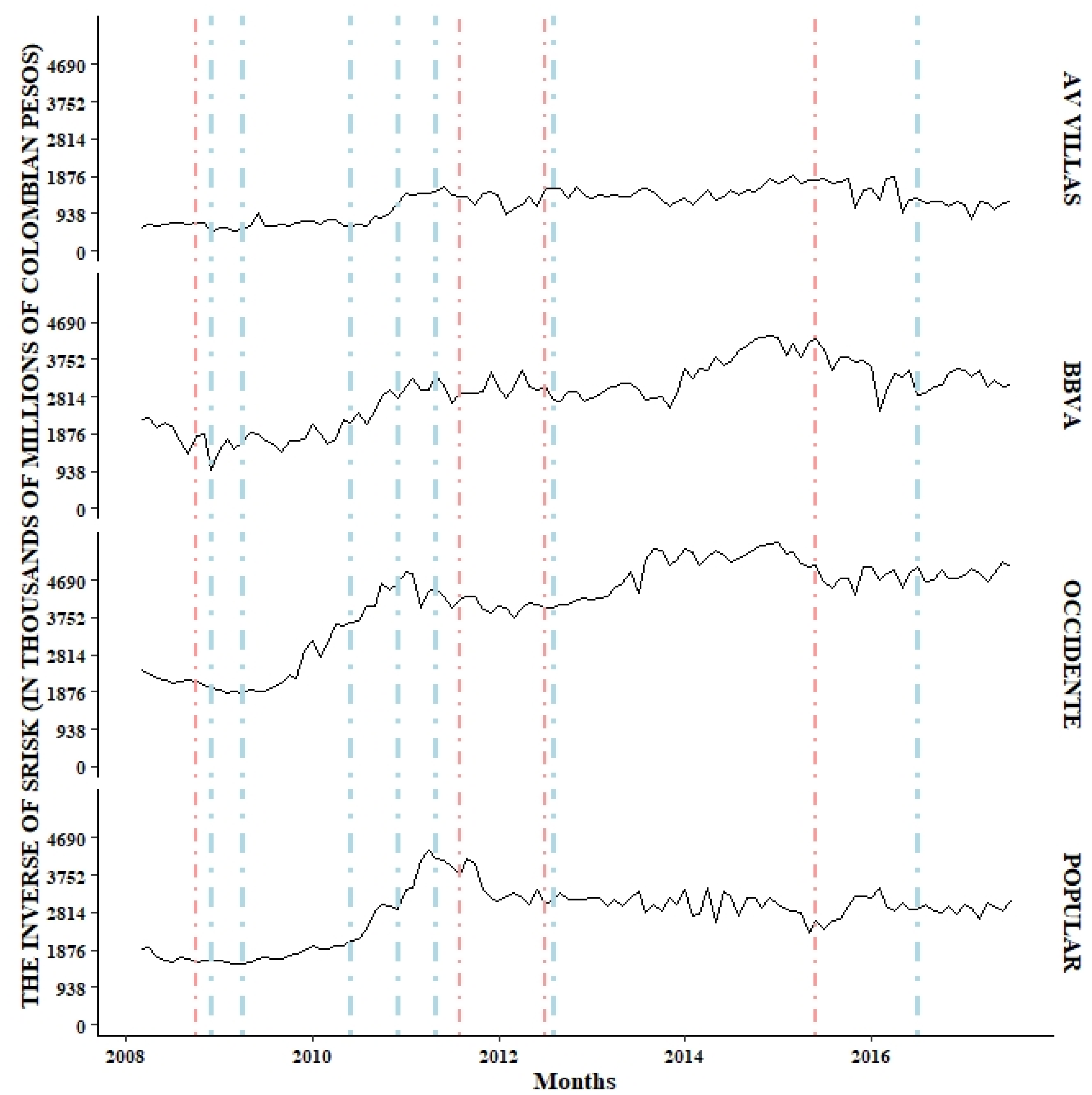
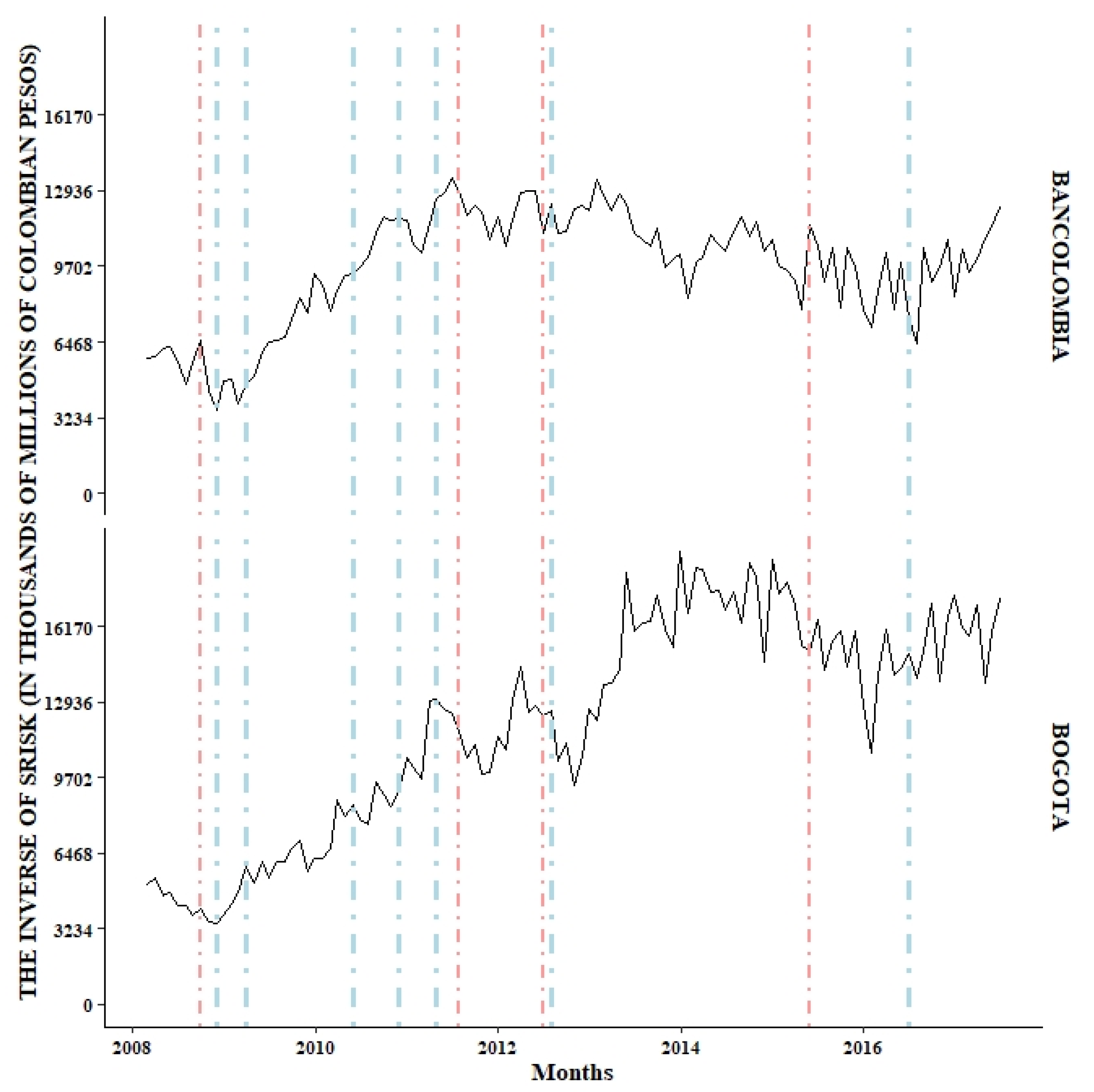
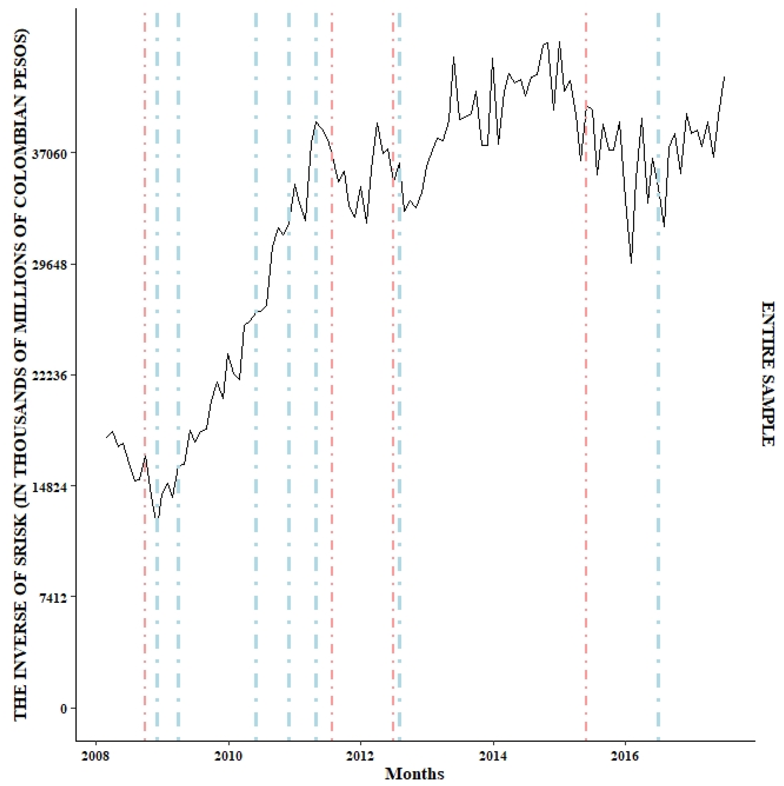
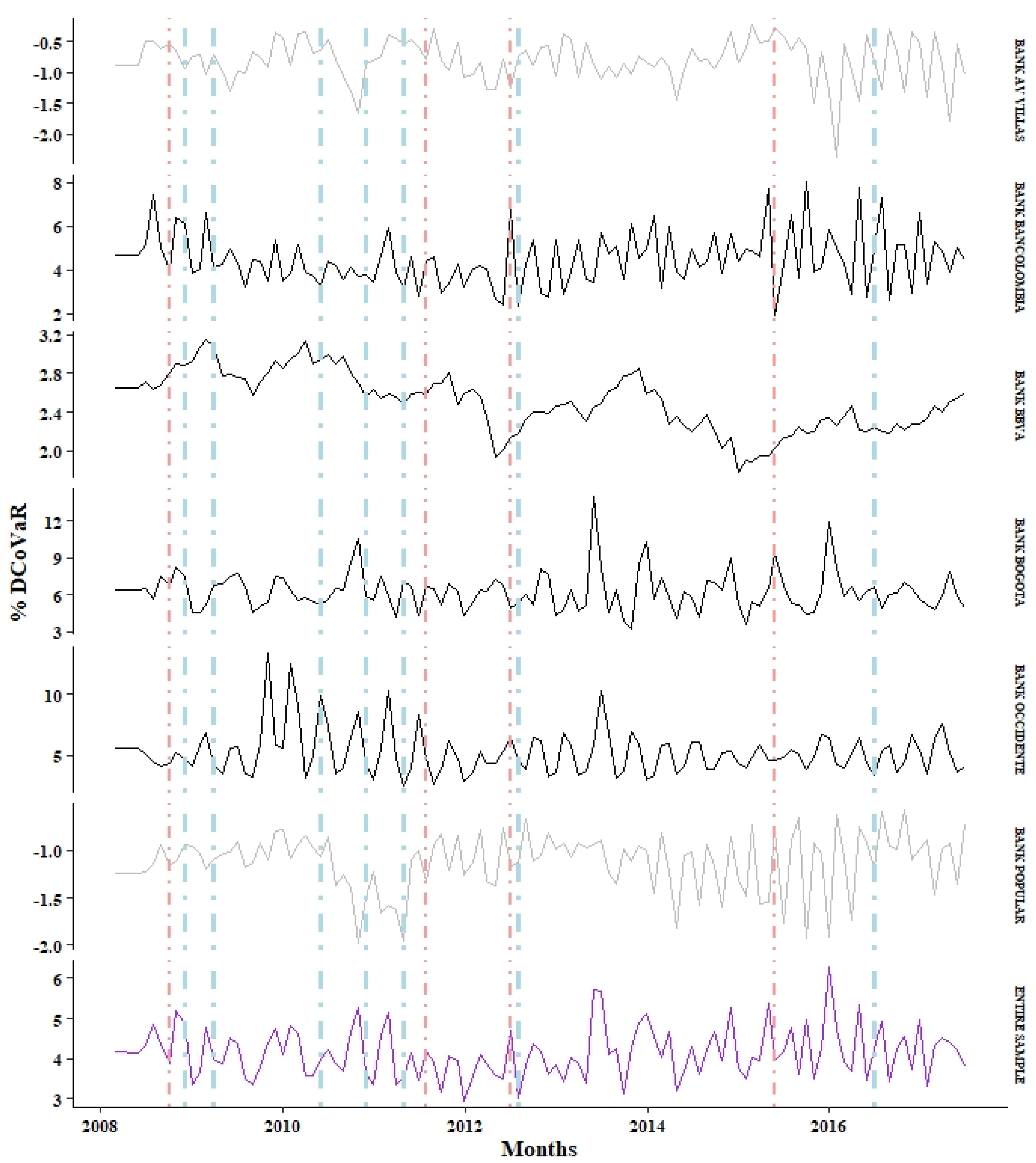
The behavior of the different risk measures was assessed to address the issue related to the realization of a systemic crisis in the Colombian banking sector; the results are presented in Table 4 and Figure 2, Figure 3, Figure 4, Figure 5 and Figure 6.
For the DCoVaR estimation, no evidence showed that the lagged state variables capture the variation in tail risk not directly related to the financial system risk exposure. This finding suggests that using the rate of variation of the value in the market of total assets with a monthly frequency significantly impacted the prominence of share prices on the behavior of the time series from stocks. We developed the methodology in search of a relative equilibrium on the information sources that make up the market value of the total assets for each institution and its respective systemic variable. Thus, the results of this risk measure correspond to dynamic behaviors without state variables.
Table 5 provides the descriptive statistics for the SRISK, DCoVaR and MES risk measures for both the banks included in the study and the respective proxy for the sample; for the SRISK indicator, the results are the sum of the individual results for the banks following the methodology described by Brownlees and Engle (2016), and for the DCoVaR and MES risk measures, the results are the weighted average of assets.
The SRISK systemic risk measure is presented separately to implement the same range for the Y-axis. However, we decided to separate the sample according to the size of each bank. The banks were separated into two samples. According to the sample, Figure 2 corresponds to the relatively small banks, these being the AV VILLAS, OCCIDENTE, POPULAR and BBVA banks. Figure 3 corresponds to the two largest banks in the Colombian banking sector, Banco Bogotá and Bancolombia. Finally, the SRISK measurement for the sample is found in Figure 4. On the other hand, in the case of the DCoVaR and MES systemic risk measures, no way was found to divide the figure based on some factor that differentiates them.
In Figure 5, the DCoVaR values for the AV Villas and Popular banks are shown in a lighter tonality than those for the other banks, a fact that is explained by the lack of evidence (statistically speaking) that extreme events (VaR) of these banks have some effect on the extreme events (VaR) of the sector. In addition, the observed results indicate an inverse relationship to that expected for this risk measure. Furthermore, this lack of agreement also transcends the MES for these banks.
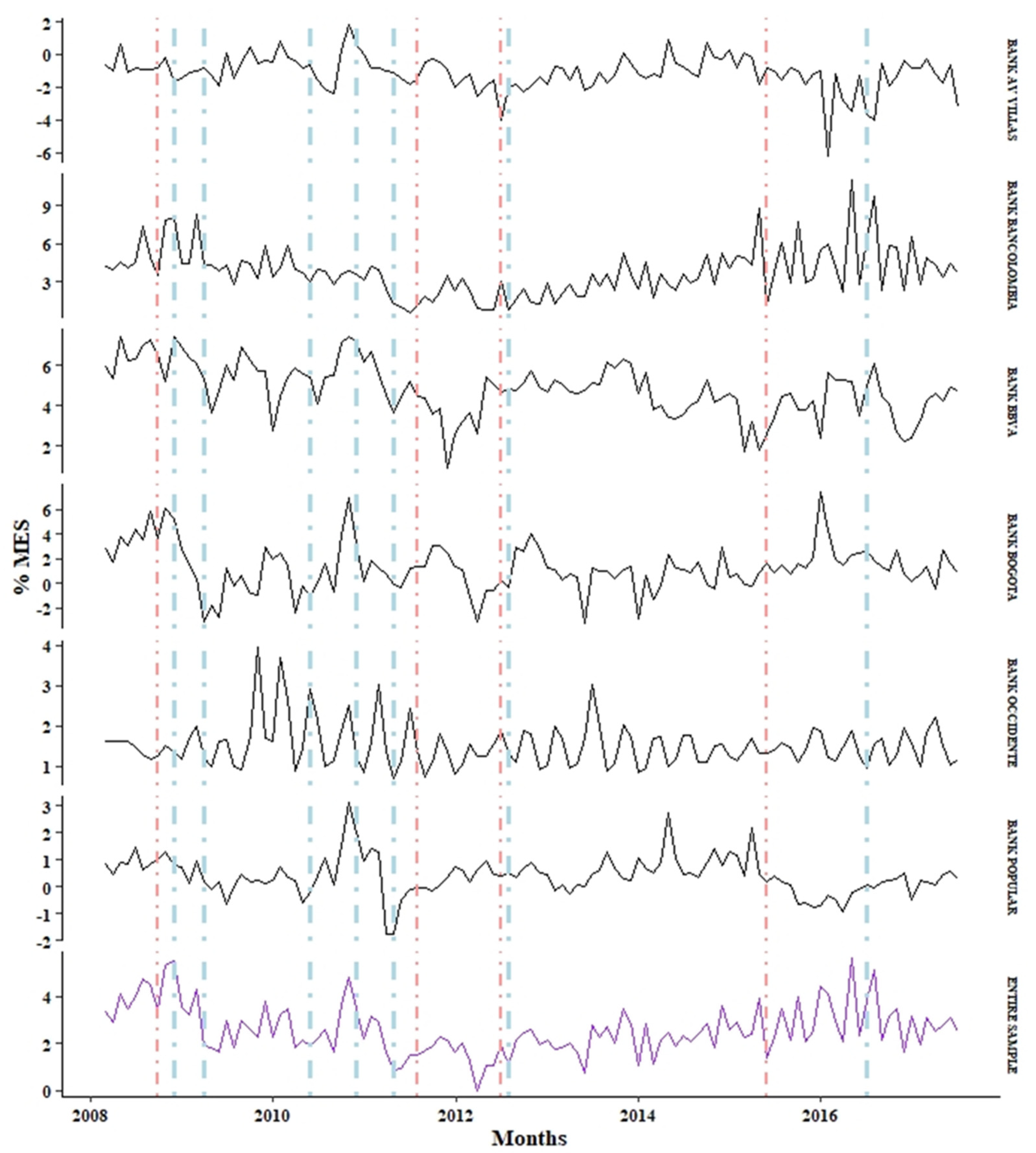
The monthly behavior of the systemic risk measures (INVERSE OF SRISK (Panel A), DCoVaR (Panel B) and MES (Panel C)) is presented for each bank and the entire sample. The lines formed by dots and vertical dashes represent the dates in which there were shocks (positive and negative) with importance in the making of investment decisions: (−) September 2008, the bankruptcy of Lehman Brothers; (+) November 2008, implementation of the Quantitative Easing policy; (+) March 2009, the central banks of large countries came together to face the crisis; (+) May 2010, the first bailout was provided (Greece, 110,000 million euros); (+) November 2010, 67,500 million euros to Ireland; (+) April 2011, 78,000 million euros to Portugal; (−) July 2011, 109,000 million euros to Greece (second bailout); (−) June 2012, Spain requested economic aid from the European Union; (+) July 2012, the European central bank declared its willingness to do everything necessary to sustain the euro; (−) May 2015, 86,000 million euros to Greece (third bailout); (+) June 2016, recovery began in Spain (Reig 2017).
There is evidence of increases in the DCoVaR and MES risk measures during periods of greater volatility in global markets; however, should these results be interpreted as realizations of systemic events in the banking sector, or are they simply the results of market shocks? The above question can be clarified when considering the estimation results for the systemic risk index of the inverse SRISK, that is, the behavior of the capital surplus in the face of significant declines in the market, providing evidence that indicates that the Colombian banking sector did not experience a systemic crisis in at least 60% of the assets managed in the sector, thus avoiding compromising the stability of the system.
Causes that could have influenced the risk measure results are the different impacts that occurred in both developed and emerging economies; the latter tend to show impacts on risk measures that are essentially due to a slowdown or reversal in capital flows that are managed through the banking sector and that, in turn, would be influenced by external factors, regardless of the economic fundamentals of the (emerging) country under consideration (Foggitt et al. 2017).
Likewise, Coleman et al. (2018) provide a critical reinterpretation of the systemic risk indicator SRISK, i.e., the different ways in which the systemic risk event was propagated during the subprime crisis and how economies were linked to this event determined the suitability and interpretation of SRISK, and therefore this indicator should be interpreted as the propensity to face losses during a crisis.
To complete this section of this research and complement the previous results, Table 5 presents the regression results using panel data for the respective risk measures, and explanatory variables addressed in the methodology. The objective of this regression is to find evidence that the explanatory variables related to characteristics such as the institution’s size, the structure of funds and the banks’ business model explain the contribution of different measures to systemic risk.
The regression using panel data considers fixed effects both for the banks and for time, and the respective standard errors provided in Table 5 were controlled for both heteroscedasticity and the serial correlation from the robust estimation of the covariance matrix. In addition, to avoid the presence of a unit root in the SRISK series, the growth rate (in logarithms) of this indicator is used. Finally, the explanatory variables were lagged to mitigate that both the dependent and independent variables were determined simultaneously (Bostandzic and Weiß 2018). Likewise, the independent variables were standardized to have a mean of zero and a standard deviation of one, thus facilitating the results’ interpretation.
In Table 5, the rows show the explanatory variables, and columns 2, 3 and 4 show the dependent variable in the regression. For the inverse SRISK, the natural logarithm of the assets and leverage were not considered because these variables are inputs for the construction of the SRISK. Below the estimated coefficients are their respective standard errors. Finally, ***, **, and * represent statistical significance at the levels of 1, 5 and 10%, respectively.
The results in Table 5 indicate that most of these variables do not significantly influence the behavior of the risk measures implemented, except for the long-term financing index, which has a significant influence on the DCoVaR risk measure. Considering the above, increasing one standard deviation in the long-term financing index decreases the DCoVaR risk measure by 25 basis points. Despite having statistical significance, the above result economically presents an incongruence between the logic of this variable and its relationship with the risk measure.
In general, the three configurations of the panel data regressions show a poor fit that the R 2 and the R 2 adjusted evidence; however, the most critical finding is that the variables present in the regressions, for the case studied herein, do not explain the results observed in the measures of systemic risk, evidence that would support a systemic scenario in the Colombian banking sector through the channels identified as promoters of systemic contributions.

6. Concluding Remarks

This paper proposes a methodology for measuring systemic risk in the banking system. The methodology estimates three systemic risk measures widely referenced in academic papers after the subprime crisis, known as DCoVaR, MES and SRISK systemic risk index. These measures individually tend to capture characteristics of systemic risk events. Therefore, the combined use would better understand and identify the causes or triggers of systemic risk in the Colombian banking sector. The proposed methodology has been tested in the Colombian banking system to determine if this sector presented a systemic crisis between February 2008 and June 2017. Similarly, the banks’ characteristics would have to support the contribution to the sector’s systemic risk.
We found evidence that a systemic event would not have materialized in the Colombian banking sector. The conclusion was provided by the SRISK systemic risk index results, which capture a particular bank’s undercapitalization in the face of the prolonged market downturn. The results showed that none of the banks considered presented a scenario of undercapitalization, implying that the economic losses imposed, mainly due to the subprime crisis, failed to endanger the stability of the Colombian banking system.
Finally, the research results that seek to determine the explanatory power of the variables used as proxies of the characteristics identified as causing the systemic importance of an institution showed that these would not be explaining the behavior of the risk measures. This result would reinforce the conclusion of the absence of a systemic risk scenario in the Colombian banking sector and that the observed results in the risk averages were the product of the external impacts to which the sector was exposed.
For methodological terms, it is essential to point out that the configuration of a monthly frequency for the analysis of systemic risk measures could be generating a Loss of explanatory power by the state variables evaluated for the DCoVaR modeling. On the other hand, we found that the mechanisms identified as drivers of systemic risk did not explain the behavior of the risk measures obtained in this work. The need to exhaustively evaluate the mechanisms by which both direct and indirect impacts, coming from the crisis suppresses, interact with the financial and regulatory systems of the Colombian economy by proposing a topic of interest to be developed. However, we consider that the preceding does not distort the results of the risk measurements implemented in this study, but rather, it is a reflection of the complexity that sustains this type of risk for both local and international financial systems.
Determining that the presence of systemic risk in the Colombian banking sector was not configured during the sample does not imply that these results should be interpreted in a wrong way that leads to thinking that the Colombian banking sector is prepared to face any risk arising from the international context. On the contrary, the subprime crisis scenario reveals the growing dynamism of financial systems, which poses new challenges for the administration and management of risk both at the institutional level and for financial regulatory institutions and the central bank. For this reason, it is necessary to carry out the consolidation of joint work for the appropriate schematization to address the mechanisms that trigger instability within the national financial sector, in search of safeguarding not only its stability and solidity, but also the productive sector of the country that is today more exposed to the dynamics presented by the financial systems, mainly national.
The results observed through the SRISK systemic risk index consistently respond to the events observed during and after the subprime crisis. In this way, this index is postulated with a tool that could be implemented to base or complement an early warning indicator for the Colombian economy, since its implementation in this research adequately captured the periods in which the sector was more affected by the events of greater relevance in the international context.

Author Contributions

Conceptualization, O.R.-E. and J.W.E.; methodology, O.R.-E.; software, O.R.-E.; validation, O.R.-E., J.W.E. and D.F.M.; formal analysis, J.W.E.; investigation, O.R.-E.; resources, O.R.-E.; data curation, O.R.-E.; writing—original draft preparation, J.W.E.; writing—review and editing, J.W.E.; visualization, O.R.-E., supervision, J.W.E.; project administration, J.W.E. and D.F.M.; funding acquisition, D.F.M. All authors have read and agreed to the published version of the manuscript.

Funding

This research received no external funding.

Conflicts of Interest

The authors declare no conflict of interest.

Appendix A

Variable NameDefinitionData Source
VIXVIX measures market expectation of near-term volatility conveyed by stock index option pricesFederal Reserve Bank of St. Louis, https://fred.stlouisfed.org (accessed on 27 January 2020)
LIQSPRShort-term liquidity margin. Difference between three-month repo rate and three-month treasury bill rate.Federal Reserve Bank of St. Louis, https://fred.stlouisfed.org (accessed on 27 January 2020)
TBR3MChange in the three-month treasury bill rate.Federal Reserve Bank of St. Louis, https://fred.stlouisfed.org (accessed on 27 January 2020)
YIESPRChange in the slope of the returns curve. Spread between ten-year and three-month treasury bill rate.Federal Reserve Bank of St. Louis, https://fred.stlouisfed.org (accessed on 27 January 2020)
CRESPRChange in the credit spread between BAA-rated bonds and treasury bill rate (both with a maturity of ten years).Federal Reserve Bank of St. Louis, https://fred.stlouisfed.org (accessed on 27 January 2020)
VOLTRMConditional volatility of the representative foreign exchange rate returns of the Colombian foreign exchange market. Obtained from an ARMA-EGARCH (3.4–7.2) model.Own calculations with data obtained from the Banco de la república de Colombia.
VOLCOLGConditional volatility of the Colombia’s stock market index returns. Obtained from an ARMA-EGARCH (5.3–7.1) model.Own calculations with data obtained from the Banco de la república de Colombia.
VOLTESConditional volatility of the returns of Colombia’s treasury bills index (IDXTES). Obtained from an ARMA-EGARCH (3.4–6.3) model.Own calculations with data obtained from the Banco de la república de Colombia.
Banks’ characteristics
Total AssetsNatural logarithm of the asset’s book value.Own calculations with data obtained from the managerial indicators published by the Superintendencia Financiera de Colombia.
LeverageIt corresponds to the quasi-market value of assets divided by the market value of equity, where the quasi-market value of assets is the book value of assets minus book value of equity + market value of equity (Acharya et al. 2017).Own calculations with data obtained from the managerial indicators published by the Superintendencia Financiera de Colombia.
Operating income different from interestsOperating income different from interest divided by total interest income.Own calculations with data obtained from the managerial indicators published by the Superintendencia Financiera de Colombia.
PortfolioParticipation of gross portfolio in total assets. This variable is calculated as the division of the gross portfolio by total assets.Own calculations with data obtained from the managerial indicators published by the Superintendencia Financiera de Colombia.
Portfolio provisionNatural logarithm of the portfolio provision.Own calculations with data obtained from the managerial indicators published by the Superintendencia Financiera de Colombia.
Long-term financing indexIndicator that captures the need to finance short-term debts with long-term resources (assets). It is obtained by dividing the subtraction of the obligations and short-term assets by the long-term assets.Own calculations with data obtained from the managerial indicators published by the Superintendencia Financiera de Colombia.
DepositsCorresponds to the division of total deposits by total liabilities.Own calculations with data obtained from the managerial indicators published by the Superintendencia Financiera de Colombia.
Source: Owner.

Appendix B

Quantile Regression
The econometric tool used to capture the codependency between institutions and the system is the Quantile Regression. This is considered adequate according to Arias et al. (2010), since:
This methodology provides a more extensive analysis than ordinary least squares because it estimates the relationship between random variables considering different quantiles. (…) Furthermore, this is a methodology that can be easily estimated for a large number of independent variables (p. 4).
This Regression method also approximates the different risk scenarios since it enables the evaluation of specific quantiles, thus capturing a large part of the states of nature captured by the sample used. A low quantile of the distribution is taken into account to estimate the CoVaR since it is in these small quantiles that financial stress episodes materialize; for this reason, the Regression by quantiles is convenient and applicable.
In general, estimating a Regression by quantiles consists of minimizing the sum of the residuals, weighted asymmetrically by a function that depends on the analyzed quantile τ . That is, the τ Quantile Regression, where 0 < τ < 1 . The above can be represented as a solution for the following expression:
m i n β t   ρ τ ( y t f ( x t , β ) )
where y t is the dependent variable, f ( x t , β ) represents a linear function of the parameters and variables used to explain the behavior of y t and ρ τ represents the weight assigned to each observation, depending on the quantile τ analyzed. In the methodology proposed by Koenker and Bassett (1978), they propose the following representation for Equation (A1):
m i n β   [ t { t : y t f ( x t , β ) } τ | y t f ( x t , β ) | + t { t : y t < f ( x t , β ) } ( 1 τ ) | y t f ( x t , β ) | ]

Appendix C

Specifications for the Modeling of Variance and Conditioned Dynamic Correlations (DCC)
The equation to capture the time variation of volatility follows the structure of the exponential GARCH model (EGACH) developed by Nelson (1991), which presents a solution to the problems associated with pessimistic estimates of the variance parameters. This specification makes it possible to capture the differential effect observed in shocks from both the “bad” and the “good” news on the behavior and magnitude of volatility, facts not captured by the standard ARCH/GARCH models because in these the conditional variance is not affected by the sign of the errors of past periods.
The equation of the EGARCH model for the volatility dynamics follows the following structure:
ln ( σ t 2 ) = ω + i = 1 q [ α i ϵ t i 2 + γ i ( | ϵ t i 2 | E ( | ϵ t i | ) ) ] + i = 1 p β i ln ( σ t i 2 )
From Equation (A3), we have that the shocks of positive returns (“Good news”) have α i + γ i impacts on the volatility of the return, while a negative shock in the returns (“bad news”) has a shock of α i γ i on the volatility of the return. The DCC conditioned dynamic correlation model specification uses volatility-adjusted returns as follows:
i t = r i t σ i t ,           m t = r m t σ m t
C o r ( i t m t ) = R t = [ 1 ρ i t ρ i t 1 ] = d i a g ( Q i t ) 1 2 d i a g ( Q i t ) 1 2
where Q i t is also called the pseudo correlation matrix, in this way, the DCC model then specifies the dynamics of the Q i t pseudo-correlation matrix as:
Q i t = ( 1 α c i β c i ) S i + α c i   [ i t 1 m t 1 ]   [ i t 1 m t 1 ] + β c i Q i t 1
where S i is the matrix of unconditional correlations of the adjusted returns of the firm and the market, the model is estimated in two steps through the quasi maximum likelihood estimation. For more details on the estimation of this model, refer to Engle (2002).

References

  1. Acharya, Viral V. 2009. A theory of systemic risk and design of prudential bank regulation. Journal of Financial Stability 5: 224–55. [Google Scholar] [CrossRef]
  2. Acharya, Viral V., Lasse H. Pedersen, Thomas Philippon, and Matthew Richardson. 2017. Measuring systemic risk. The Review of Financial Studies 30: 2–47. [Google Scholar] [CrossRef]
  3. Aparicio, Mónica, Alexandra Heredia, Camilo José Hernández, Juan Carlos Quintero, and Olga Esperanza Serna. 2012. Crisis Financieras Sistémicas en Colombia y Contraste con el Escenario Actual. Documento de Investigación. Colombia: Fogafin. [Google Scholar]
  4. Arias, Mauricio, Juan Carlos Mendoza-Gutiérrez, and David Pérez-Reyna. 2010. Applying covar to measure systemic market risk: The colombian case. Temas de Estabilidad Financiera 47: 1–16. [Google Scholar]
  5. Berger, Allen N., Jin Cai, Raluca A. Roman, and John Sedunov. 2021. Supervisory enforcement actions against banks and systemic risk. Journal of Banking & Finance. [Google Scholar] [CrossRef]
  6. Bostandzic, Denefa, and Gregor N. F. Weiß. 2018. Why do some banks contribute more to global systemic risk? Journal of Financial Intermediation 35: 17–40. [Google Scholar] [CrossRef]
  7. Boucher, Christophe M., Patrick S. Kouontchou, Bertrand B. Maillet, and O. Scaillet. 2013. The Co-CoVaR and Some Other Fair Systemic Risk Measures with Model Risk Corrections. Available online: www.systemic-riskhub.org/papers/selectedworks/BoucherKouontchouMailletScaillet_2013_fullpaper.pdf (accessed on 27 January 2020).
  8. Brownlees, Christian, and Robert F. Engle. 2016. SRISK: A conditional capital shortfall measure of systemic risk. The Review of Financial Studies 30: 48–79. [Google Scholar] [CrossRef]
  9. Cabrera-Rodríguez, Wilmar Alexander, Jorge Luis Hurtado-Guarín, Miguel Morales, and Juan Sebastián Rojas-Bohórquez. 2014. A Composite Indicator of Systemic Stress (CISS) for Colombia. Borradores de Economía; No. 826. Colombia: Banco de República. [Google Scholar]
  10. Cáceres, José Antonio. 2009. Colombia ante la crísis financiera global. Revista Escuela de Administración de Negocios 65: 5–30. [Google Scholar] [CrossRef]
  11. Castelao, Silvina, Sofía Palmigiani, and Patricia Lampes. 2013. Riesgo Sistémico: Una Aproximación Para el Sistema Bancario Uruguayo. No. 2013003. Montevideo: BCU. [Google Scholar]
  12. Coleman, Thomas F., Alex LaPlante, and Alexey Rubtsov. 2018. Analysis of the SRISK measure and its application to the Canadian banking and insurance industries. Annals of Finance 14: 547–70. [Google Scholar] [CrossRef]
  13. Davydov, Denis, Sami Vähämaa, and Sara Yasar. 2021. Bank liquidity creation and systemic risk. Journal of Banking & Finance 123: 106031. [Google Scholar]
  14. Drakos, Anastassios A., and Georgios P. Kouretas. 2015. Bank ownership, financial segments and the measurement of systemic risk: An application of CoVaR. International Review of Economics & Finance 40: 127–40. [Google Scholar]
  15. Duan, Yuejiao, Sadok El Ghoul, Omrane Guedhami, Haoran Li, and Xinming Li. 2021. Bank systemic risk around COVID-19: A cross-country analysis. Journal of Banking & Finance 133: 106299. [Google Scholar]
  16. Engle, Robert. 2002. Dynamic conditional correlation: A simple class of multivariate generalized autoregressive conditional heteroskedasticity models. Journal of Business & Economic Statistics 20: 339–50. [Google Scholar]
  17. Estrada, Dairo Ayiber, and Daniel Esteban Osorio-Rodríguez. 2006. A market risk approach to liquidity risk and financial contagion. Revista Ensayos Sobre Política Económica 24: 242–71. [Google Scholar] [CrossRef]
  18. Foggitt, Gregory M., Andre Heymans, Gary W. van Vuuren, and Anmar Pretorius. 2017. Measuring the systemic risk in the South African banking sector. South African Journal of Economic and Management Sciences 20: 1–9. [Google Scholar] [CrossRef] [Green Version]
  19. Furfine, Craig H. 2003. Interbank exposures: Quantifying the risk of contagion. Journal of Money, Credit and Banking 35: 111–28. [Google Scholar] [CrossRef]
  20. Grilli, Ruggero, Gabriele Tedeschi, and Mauro Gallegati. 2015. Markets connectivity and financial contagion. Journal of Economic Interaction and Coordination 10: 287–304. [Google Scholar] [CrossRef]
  21. Group of Ten. 2001. Report on Consolidation in the Financial Sector. Available online: https://www.imf.org/external/np/g10/2001/01/Eng/index.htm (accessed on 27 January 2020).
  22. Guerra, Solange Maria, Thiago Christiano Silva, Benjamin Miranda Tabak, Rodrigo Andrés de Souza Penaloza, and Rodrigo César de Castro Miranda. 2016. Systemic risk measures. Physica A: Statistical Mechanics and its Applications 442: 329–42. [Google Scholar] [CrossRef]
  23. International Monetary Fund. 2010. Annual Report 2010 Supporting a Balanced Global Recovery. Available online: https://www.imf.org/~/media/Websites/IMF/imported-flagship-issues/external/pubs/ft/ar/2010/eng/pdf/_ar10engpdf.ashx (accessed on 1 September 2021).
  24. Kleinow, Jacob, Fernando Moreira, Sascha Strobl, and Sami Vähämaa. 2017. Measuring systemic risk: A comparison of alternative market-based approaches. Finance Research Letters 21: 40–46. [Google Scholar] [CrossRef] [Green Version]
  25. Koenker, Roger, and Gilbert Bassett Jr. 1978. Regression quantiles. Econometrica: Journal of the Econometric Society 1: 33–50. [Google Scholar] [CrossRef]
  26. Laeven, Luc, Lev Ratnovski, and Hui Tong. 2016. Bank size, capital, and systemic risk: Some international evidence. Journal of Banking & Finance 69: S25–S34. [Google Scholar]
  27. Laverde, Mariana, and Javier Gutiérrez-Rueda. 2012. ¿Cómo Caracterizar Entidades Sistémicas? Medidas de Impacto Sistémico Para Colombia. Temas de Estabilidad Financiera, No. 65. Colombia: Banco de República. [Google Scholar]
  28. León, Carlos, and Clara Machado. 2011. Designing an Expert Knowledge-Based Systemic Importance Index for Financial Institutions. Borradores de Economía, No. 669. Colombia: Banco de República. [Google Scholar]
  29. León, Carlos, Clara Machado, Miguel Sarmiento, Freddy Cepeda, Orlando Chipatecua, and Jorge Cely. 2011. Riesgo sistémico y estabilidad del sistema de pagos de alto valor en Colombia: Análisis bajo topología de redes y simulación de pagos. Revista Ensayos Sobre Política Económica (ESPE) 29: 109–75. [Google Scholar] [CrossRef]
  30. Lin, Edward MH, Edward W. Sun, and Min-Teh Yu. 2018. Systemic risk, financial markets, and performance of financial institutions. Annals of Operations Research 262: 579–603. [Google Scholar] [CrossRef]
  31. López-Espinosa, Germán, Antonio Moreno, Antonio Rubia, and Laura Valderrama. 2012. Short-term wholesale funding and systemic risk: A global CoVaR approach. Journal of Banking & Finance 36: 3150–62. [Google Scholar]
  32. Luciano, Elisa, and Clas Wihlborg. 2018. Financial synergies and systemic risk in the organization of bank affiliates. Journal of Banking & Finance 88: 208–24. [Google Scholar]
  33. Meuleman, Elien, and Rudi Vander Vennet. 2020. Macroprudential policy and bank systemic risk. Journal of Financial Stability 47: 100724. [Google Scholar] [CrossRef] [Green Version]
  34. Nelson, Daniel B. 1991. Conditional heteroskedasticity in asset returns: A new approach. Econometrica: Journal of the Econometric Society 59: 347–70. [Google Scholar] [CrossRef]
  35. Reig, Paula. 2017. Diez Años de Crisis en 24 Acontecimientos Clave. Available online: https://www.bbva.com/es/diez-anos-crisis-24-acontecimientos-clave/ (accessed on 23 March 2020).
  36. Silva, Walmir, Herbert Kimura, and Vinicius Amorim Sobreiro. 2017. An analysis of the literature on systemic financial risk: A survey. Journal of Financial Stability 28: 91–114. [Google Scholar] [CrossRef]
  37. Silva-Buston, Consuelo. 2019. Systemic risk and competition revisited. Journal of Banking & Finance 101: 188–205. [Google Scholar]
  38. Tobias, Adrian, and Markus K. Brunnermeier. 2011. CoVaR. No 17454, NBER Working Papers. Cambridge: National Bureau of Economic Research, Inc., Available online: https://econpapers.repec.org/repec:nbr:nberwo:17454 (accessed on 23 April 2020).
  39. Tobias, Adrian, and Markus K. Brunnermeier. 2016. CoVaR. The American Economic Review 106: 1705. [Google Scholar]
  40. V-Lab. n.d. Dynamic MES. Available online: https://vlab.stern.nyu.edu/docs/srisk/MES (accessed on 24 April 2020).
  41. Vogl, Christian. 2015. Systemic Risk Measurement in the Eurozone—A Multivariate GARCH Estimation of CoVaR. Lund: Lund University. [Google Scholar]
  42. Zedda, Stefano, and Giuseppina Cannas. 2020. Analysis of banks’ systemic risk contribution and contagion determinants through the leave-one-out approach. Journal of Banking & Finance 112: 105160. [Google Scholar]
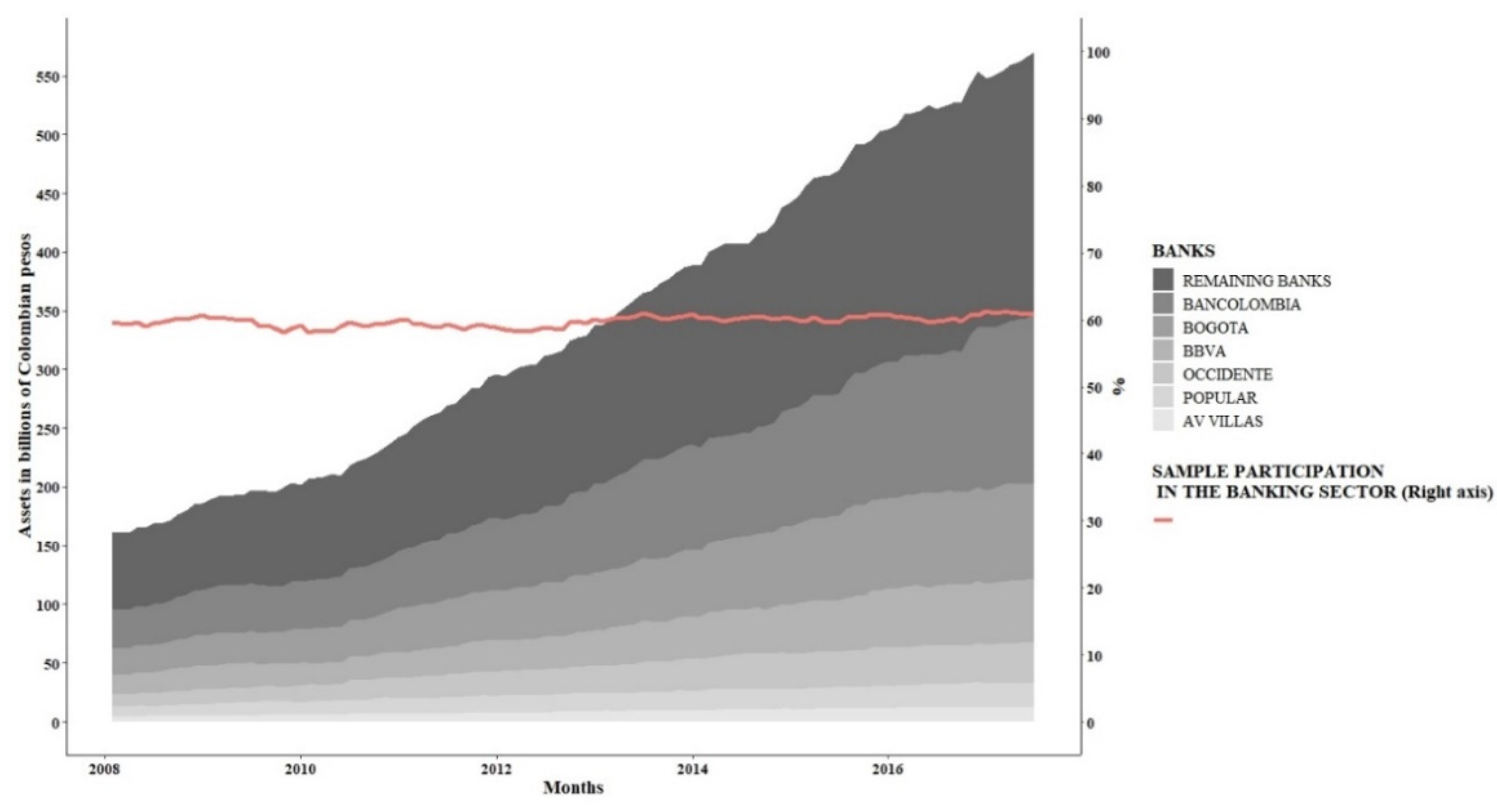
Figure 1. Participation in the level of assets of the selected sample on the sector. Source: Owner.
Risks 10 00022 g001
Figure 2. Monthly behavior of systemic risk measures. Source: owner.
Risks 10 00022 g002
Figure 3. Monthly behavior of the SRISK systemic risk measure for BANCOLOMBIA and BOGOTÁ banks. Source: owner.
Risks 10 00022 g003
Figure 4. Monthly behavior of the SRISK systemic risk measure for the entire sample. Source: owner.
Risks 10 00022 g004
Figure 5. Monthly behavior of the DCoVaR systemic risk measure for both banks and the entire sample. Source: owner.
Risks 10 00022 g005
Figure 6. Monthly behavior of the MES systemic risk measure for both banks and the entire sample. Source: Owner.
Risks 10 00022 g006
Table 1. Descriptive statistics of the market value growth rate of total assets and the system variable.
Descriptive StatisticsNBanks
AV VILLASBANCOLOMBIABBVABOGOTÁOCCIDENTEPOPULAR
BankSystemBankSystemBankSystemBankSystemBankSystemBankSystem
Mín113−0.428−0.336−0.514−0.178−0.302−0.236−0.142−0.212−0.095−0.314−0.197−0.267
1st Qu.113−0.049−0.038−0.056−0.031−0.059−0.023−0.02−0.023−0.016−0.029−0.027−0.033
Median1130.010.0280.0510.01−0.010.0170.0060.0220.0020.0260.0030.024
Average1130.0290.0270.030.0170.0140.0210.010.0210.0090.0240.0040.022
3rd Qu.1130.0730.1040.1170.0690.0560.0730.0380.0750.0230.0870.0390.07
Max11317760.3620.5940.2840.3410.240.1570.2980.1990.3260.2520.258
Source: Owner.
Table 2. ARMA and EGARCH results for the sample data.
SpecificationAV VILLASBANCOLOMBIABBVABOGOTÁOCCIDENTEPOPULAR
SystemBank SystemBank SystemBank SystemBank SystemBank SystemBank
ARMAAR1−0.034479 *** (0.000002)−0.246957 *** (0.000079) −0.049502 *** (0.000090−0.214773 *** (0.000130)0.302472 *** (0.000307)−1.07579 *** (0.000134) −1.026864 *** (0.001008)−0.404966 *** (0.000017)−0.103862 *** (0.000009)
AR20.842407 *** (0.000113)0.151093 *** (0.000241) −0.195470 *** (0.000173)0.824432 *** (0.000828)−0.726260 *** (0.002171)−0.94786 *** (0.000556) −1.095858 *** (0.001594)−0.731353 *** (0.000040)
AR3 0.041250 *** (0.000139) −0.144043 *** (0.000095)
MA10.275944 *** (0.000001) 0.224597 *** (0.000269) 0.470256 *** (0.000408)−0.133322 *** (0.000054)1.05083 *** (0.003667)−0.25046 *** (0.000009)1.125084 *** (0.000669)0.533917 *** (0.000044) −0.046343 *** (0.000009)
MA2−1.095661 *** (0.000231) −0.991695 *** (0.000063)0.538468 *** (0.000342)0.86165 *** (0.001624) 1.234945 *** (0.000874)0.686710 *** (0.000009) −0.076016 *** (0.000005)
MA3−0.240641 *** (0.000104) −0.188052 *** (0.000150)0.278034 *** (0.000166) 0.292615 *** (0.000109)0.229717 *** (0.000012) −0.073302 *** (0.000001)
MA40.355981 *** (0.000014) 0.264615 *** (0.000076)−0.447289 *** (0.001104) −0.184071 *** (0.000318) 0.051772 *** (0.000028)
EGARCHARCH10.799366 *** (0.000303)0.012710 *** (0.000031)0.246493 *** (0.000754)−0.576275 *** (0.000133)0.605561 *** (0.000035)−0.069722 *** (0.000166)0.33965 *** (0.001264)0.44333 *** (0.000105)0.537437 *** (0.000114)0.422964 *** (0.001229)0.011183 *** (0.000047)0.149429 *** (0.000013)
ARCH2−0.579092 *** (0.000059)0.323211 *** (0.000908)−0.384483 *** (0.001015)0.140552 *** (0.000034)−0.789385 *** (0.000009) 0.132865 *** (0.000190) 0.154661 *** (0.000050)0.157589 *** (0.000014)
ARCH3−0.451457 *** (0.000105)−0.853260 *** (0.000486) 0.702936 *** (0.000578)0.219627 *** (0.000737) −0.104234 *** (0.000032)
ARCH40.471059 *** (0.000138) −0.376674 *** (0.000009)
GARCH10.644798 *** (0.000292)0.726499 *** (0.000853)0.997655 *** (0.009199)0.036037 *** (0.000044)0.540945 *** (0.000161)0.961643 *** (0.003489)0.35768 *** (0.001203)0.41782 *** (0.000115)−0.042545 *** (0.000041)0.815780 *** (0.000302)−0.125789 *** (0.000047)−0.227812 *** (0.000061)
GARCH2 −0.107191 *** (0.000058)−0.022221 *** (0.000009)0.534309 *** (0.000690)−0.490466 *** (0.000137) −0.21096 *** (0.000147)−0.77307 *** (0.000482)−0.328719 *** (0.000051)−1.000000 *** (0.000075)0.973641 *** (0.001867)−0.009186 *** (0.000001)
GARCH3 0.787467 *** (0.001844) 0.296964 *** (0.000203)0.688145 *** (0.000609) 0.70607 *** (0.000028)0.53256 *** (0.000298)0.493064 *** (0.000072)0.712506 *** (0.000023)0.036081 *** (0.000036)0.734146 *** (0.000337)
GARCH4 −0.748643 *** (0.001662) −0.62262 *** (0.001066)−0.86264 *** (0.000495)0.037023 *** (0.000091)−0.066404 *** (0.000157)−0.682825 *** (0.000912)−0.129795 *** (0.000016)
GAMMA1−0.885067 *** (0.000101)0.996195 *** (0.000574)0.115575 *** (0.000175)0.632487 *** (0.000820)−0.420413 *** (0.000873)−0.246882 *** (0.001143)1.15198 *** (0.032347)1.21458 *** (0.000511)0.721123 *** (0.000233)0.930880 *** (0.000041)1.589955 *** (0.001813)0.459014 *** (0.000084)
GAMMA20.029432 *** (0.000030)−0.943253 *** (0.000887)−0.331180 *** (0.001007)−1.079320 *** (0.000993)−0.417899 *** (0.000043) 1.408392 *** (0.000516) 0.076924 *** (0.000026)1.140554 *** (0.000129)
GAMMA31.135463 *** (0.000306)−0.448216 *** (0.000036) −1.413676 *** (0.000585)−0.140913 *** (0.000193) −0.888913 *** (0.001216)
GAMMA4−1.427526 *** (0.0000499 1.201497 *** (0.002484)
Source: Owner.
Table 3. Estimated results for the data sample.
SpecificationsBanks
AV VILLASBANCOLOMBIABBVABOGOTÁOCCIDENTEPOPULAR
SystemBankSystemBankSystemBankSystemBankSystemBankSystemBank
Statistic of Weighted ARCH LM TestsLAG3.562 * (8)3.006 * (6)2.149 (5)0.2935 (8)0.3971 (7)0.8164 (3)0.1252 (6)0.006104 (6)2.378 (7)0.05129 (6)0.01764 (8)0.004192 (7)
LAG5.027 (10)4.306 (8)2.688 (7)1.3683 (10)1.5182 (9)0.9351 (5)0.4744 (8)0.108698 (8)2.679 (9)0.34029 (8)1.50173 (10)0.008476 (9)
LAG6.327 (12)4.751 (10)3.553 (9)1.8888 (12)2.8858 (11)1.656 (7)1.0434 (10)0.211909 (10)4.512 (11)3.94416 (10)1.72761 (12)0.013002 (11)
Statistic of Weighted Ljung-Box Test on Standardized ResidualsLAG(1)0.3450.2250.50310.011740.47660.31040.91130.66870.0030.13060.79950.07855
LAG [2 x (p + q) + (p + q) − 1]9.1451.4971.16331.435779.17055.77345.60352.18827.9316.90931.32963.1782
LAG [4 x (p + q) + (p + q) − 1]15.9272.5222.28553.1830318.069515.55138.84233.860613.37611.97682.46116.2216
t-value of Sign Bias TestSign Bias0.26251.92338 *0.4741.01721.19450.19731.06920.61550.40140.56280.71370.9539
−Sign Bias0.35570.312160.015920.218370.11440.44380.49760.0610.60780.1520.7830.2512
+Sign Bias1.2890.050670.244860.027481.17680.18971.60550.25990.62371.5321.4761.2071
Joint Effect2.0436.30388 *0.338063.162042.05180.24383.24511.48171.09962.37093.08697.3373 *
Statistic of Adjusted Pearson Goodness-of-Fit TestGroup 2025.2324.5224.5223.1116.7310.0113.914.6118.8613.5517.4419.92
Group 3032.7530.129.5726.3836.4720.0122.6629.0427.9722.1327.4420.54
Group 4042.448.7740.2731.7836.7327.5328.9530.3745.2333.1937.4436.73
Group 5047.6258.2437.8848.542.73744.0831.247.6239.6547.6237.88
Dynamic Conditional Correlation (DCC)p10.051755 ** (0.025315)0.039008 ** (0.015635) 0.086556 *** (0.004175) 0.25804 *** (0.059624)0.000000 ** (0.000000)0.063595 *** (0.021299)
q10.486054 *** (0.185008)0.860154** (0.380315)0.461762 ** (0.214375) 0.37346 *** (0.131889) 0.902351 *** (0.115806)0.553310 *** (0.165288)
Normal distribution YesYesYesYesYesYes
Quantile Regression (τ = 0.05)Intercept−0.13094 *** (0.01403)−0.103357 *** (0.009594)−0.10624 *** (0.01127) −0.10761 *** (0.01062) −0.13298 *** (0.01459)−0.10531 *** (0.01152)
Beta−0.03467 (0.22383)0.189388 *** (0.055078)0.20543 ** (0.07904) 0.73401 *** (0.17231)0.73588 *** (0.18341)−0.11914 (0.16436)
Table 4. Descriptive statistics of systemic risk measures.
BanksDescriptive StatisticsNSRISK%DCoVaR%MES
AV VILLASMín113454.30–2.38–6.26
1st Qu.113787.00–0.96–1.58
Median1131263.00–0.79–1.02
Average1131191.00–0.81–1.13
3rd Qu.1131496.00–0.55–0.55
Max1131891.00–0.241.80
BANCOLOMBIAMín1133593.001.930.60
1st Qu.1137959.003.662.44
Median11310,307.004.343.64
Average1139675.004.473.76
3rd Qu.11311,528.005.114.48
Max11313,455.000.8010.98
BBVAMín113966.001.780.94
1st Qu.1132298.002.274.03
Median1132981.902.544.77
Average1132888.202.514.81
3rd Qu.1133460.102.715.68
Max1134348.403.157.45
BOGOTAMín1133480.003.25–3.26
1st Qu.1138466.005.230.17
Median11312,759.006.271.20
Average11312,024.006.291.27
3rd Qu.11315,956.006.962.39
Max11319,400.0014.017.44
OCCIDENTEMín1131835.002.460.69
1st Qu.1133680.003.921.13
Median1134393.004.971.44
Average1134110.005.221.52
3rd Qu.1134988.005.891.72
Max1135624.0013.363.95
POPULARMín1131530.00–1.98–1.78
1st Qu.1132160.00–1.250.05
Median1132973.00–1.070.38
Average1132766.00–1.130.41
3rd Qu.1133182.00–0.930.82
Max1134395.00–0.583.11
SAMPLEMín11312,044.002.960.00
1st Qu.11326,491.003.661.89
Median11335,914.004.092.39
Average11332,653.004.152.60
3rd Qu.11339,109.004.563.21
Max11344,470.006.265.62
Source: owner.
Table 5. Results of the explanatory power of the characteristics of the banks.
Dependent Variables
Independent VariablesInverse of SRISKDCoVaRMES
Log-natural assets −0.001230.00625
(0.00440)(0.00630)
Leverage −0.00170−0.00023
(0.00153)(0.00110)
Long-term financing index−0.00140−0.00250 ***−0.00060
(0.00390)(0.00088)(0.00210)
Deposits−0.00986−0.00054−0.00250
(0.00626)(0.00081)(0.00270)
Other incomes different from the interest−0.00080−0.00045−0.00100
(0.00340)(0.00036)(0.00100)
Portfolio−0.001700.00011−0.00080
(0.00620)(0.00071)(0.00100)
Provisions Portfolio−0.00490−0.000570.00630
(0.02000)(0.00470)(0.00850)
Fixed effects—banksYesYesYes
Fixed effects—timeYesYesYes
Observations672452565
R20.00060.01700.0420
Adjusted R2−0.2190−0.3500−0.2252
Source: Owner.
Publisher’s Note: MDPI stays neutral with regard to jurisdictional claims in published maps and institutional affiliations.