Abstract
The question of whether environmental, social, and governance investments outperform or underperform other conventional financial investments has been debated in the literature. In this study, we compare the volatility of rates of return of selected ESG indices and conventional ones and investigate dependence between them. Analysis of tail dependence is important to evaluate the diversification benefits between conventional investments and ESG investments, which is necessary in constructing optimal portfolios. It allows investors to diversify the risk of the portfolio and positively impact the environment by investing in environmentally friendly companies. Examples of institutions that are paying attention to ESG issues are banks, which are increasingly including products that support sustainability goals in their offers. This analysis could be also important for policymakers. The European Banking Authority (EBA) has admitted that ESG factors can contribute to risk. Therefore, it is important to model and quantify it. The conditional volatility models from the GARCH family and tail-dependence coefficients from the copula-based approach are applied. The analysis period covered 2007 until 2019. The period of the COVID-19 pandemic has not been analyzed due to the relatively short time series regarding data requirements from models’ perspective. Results of the research confirm the higher dependence of extreme values in the crisis period (e.g., tail-dependence values in 2009–2014 range from 0.4820/0.4933 to 0.7039/0.6083, and from 0.5002/0.5369 to 0.7296/0.6623), and low dependence of extreme values in stabilization periods (e.g., tail-dependence values in 2017–2019 range from 0.1650 until 0.6283/0.4832, and from 0.1357 until 0.6586/0.5002). Diversification benefits vary in time, and there is a need to separately analyze crisis and stabilization periods.
1. Introduction
The pandemic has highlighted social and global inequality and spiked interests in environmental, social, and governance (ESG) investing. ESG assets reached $35.3 trillion in 2020 from around $30.7 trillion in 2018, reaching a third of current total global assets under management, according to the Global Sustainable Investment Association (http://www.gsi-alliance.org/, accessed on 18 November 2021).
According to the 2020 Trends Report, investors are considering ESG factors across USD 17 trillion of professionally managed assets, a 42% increase since 2018. Such continued growth is expected over the long term, too. Since 1995, the value of US sustainable investment assets (USD 639 billion) has increased more than 25-fold (USD 16.6 trillion in 2020), at a compound annual growth rate of 14% (US SIF 2020).
A few terms are used interchangeably to describe environmental, social, and governance investments, e.g., socially responsible investing (SRI), responsible investing, sustainable investing, and impact investing. In this paper, we understand ESG investing in terms of the ESG factors, which enhance traditional financial analysis, making it more complete.
There are some ESG factors that are helpful in the evaluation of investment performance. Investments with high ESG scores can increase rates of return, while those with poor ESG scores may inhibit these rates. One may find energy consumption, pollution, climate change, waste production, natural resource preservation (deforestation, carbon emission reduction), and animal welfare among the environmental factors. The social factors include human rights, child and forced labor, community engagement, health and safety, stakeholder relations and employee relations, customer success, data hygiene, and security. The governance factors contain the following: quality of management, board independence, conflict of interest, executive compensation, hiring and onboarding best practices, transparency, and disclosure. In this paper, we use the term ESG to refer to these indices, which include the companies that disclose these factors.
Morgan Stanley’s research on nearly 11,000 mutual funds between 2004 and 2018 indicates there is no financial trade-off in returns of sustainable funds compared to traditional ones. Moreover, sustainable funds showed lower downside risk. The number of ESG focused funds has been growing, since 2004 by 144% (Morgan Stanley, Institute for Sustainable Investing, Sustainable Reality. Analyzing Risk and Returns of Sustainable Funds, 2019. www.morganstanley.com, accessed on 18 November 2021).
A growing number of investors not only focus on the profitability of investment strategies but also look for their social value. ESG investing fulfills this goal. ESG looks at the company’s environmental, social, and governance practices, as well as traditional ones. ESG investors believe that investments in companies employing ESG practices may have a material impact on their investments’ profitability and risk. Moreover, they accept a lower return in the short term and even slightly higher risk because of the additional future value of their investment.
Considering ESG benefits in investing for economic value is not a new concept. The report “Who Cares, Wins—Connecting Financial Markets to a Changing World”, which provided guidelines for companies to incorporate ESG into their operations, was published in 2004. The first ESG index, the Domini 400 Social Index (now known as the MSCI KLD 400 Social Index), was launched in May 1990. Since then, the ESG indices have evolved to meet investors’ unique needs in investing.
ESG equity indices are used as benchmarks for ESG investment, as the underlying assets of passive ESG investment tools (such as exchange-traded funds), and as related risk-management tools (ESG index futures). ESG equity indices are usually constructed based on parent equity indices incorporating ESG investment styles. The construction process may comprise screening out the companies with negative ESG impacts and including the companies with positive ESG impacts by adjusting their relative weights. Therefore, the risk-return performances of these indices may be different from those of their parent indices with traditional investment strategies (HKEX 2020).
Making investment decisions, including portfolio construction, requires knowledge of volatility and dependence between financial time series. Determination of the dependence structure is essential for portfolio management, and the misinterpretation of the strength of this dependence can lead to wrong investment decisions. Pearson’s linear correlation coefficient is the most common and widely used correlation measure. Because of its linearity, it is a tool appropriate only for measuring the dependence between variables of elliptic distributions. In situations where empirical data are characterized by, for example, asymmetric and non-elliptic distributions, with high kurtosis or skewness, the use of linear correlation coefficient is not advisable. In such instances, copula functions are better tools for investigating the dependence structure between the time series (Messaoud and Aloui 2015).
The objective of the paper is to evaluate the attractiveness of ESG investments as a potential diversifier for conventional investments. In this study, we examine the following hypothesis:
Hypothesis 1 (H1).
ESG investments outperform conventional investments in terms of risk.
Hypothesis 2 (H2).
Asymptotic dependence increases during the crisis on the market (declines of stock market indices), stabilizing during the non-crisis periods.
There are many ESG indices; in this paper, we select five ESG indices (see Table A1 for details). Conventional stock indices are represented by the Dow Jones Industry Average (DJI) and the S&P 500 (GSPC).
Because little is known about the dependence structure between ESG and conventional investments, the contribution of this paper is to fill this research gap. The pioneering character of this research—application of tail dependence to ESG investments, is highly contributing both to the knowledge of the field as well as to the practice of assets selection in portfolio construction. The paper also contributes to improving the understanding of volatility and the (tail) dependence structure between ESG and conventional investments. By quantifying the overall and lower tail risk between these two assets, we indicate that these dependencies exist, can be quantified, and are not negligible, especially in times of crisis.
The research results confirm the higher dependence of extreme values in the crisis period (declines of indices); however, this is also due to increased volatility during this period.
The paper is structured as follows: the introduction, literature review, research methodology, data description, empirical results, discussion, conclusions, and references.
Literature Review
Managi et al. (2012) report no statistical difference in means and volatilities generated from the SRI indices and conventional indices in neither of the studied regions (the US, the UK, and Japan). Furthermore, they found strong comovements between the two indices in both regimes (bear and bull). In contrast, Ortas et al. (2014) found that in the period of the global financial crisis of 2008, social and responsible investment strategies were less risky in comparison to conventional investments.
There is no consensus in the literature as to whether ESG investments are characterized by very high returns and very low risks compared to conventional ones.
Weber and Ang (2016) analyzed the performance of an emerging market SRI index concerning its financial performance compared to conventional indices. Their results indicate that the SRI index outperformed in terms of mean return the majority of the conventional emerging market portfolios. Similarly, Verheyden et al. (2016) found that both global and developed-markets portfolios (a 10% best-in-class ESG screening approach) show higher returns, lower (tail) risk, and no significant reduction of diversification potential.
On the other hand, Giese and Lee (2019) reported no clear consensus on whether ESG criteria have enhanced risk-adjusted returns. The empirical findings in the report on ESG indices performance (HKEX 2020), indicate that many ESG indices tended to have similar, if not better, risk-return performances then their parent indices. This implies that investment in ESG indices may provide equally good or even better returns while pursuing an ethics-focused investment strategy.
Ouchen (2021) empirically verified whether the series of returns of an ESG index was less volatile than that of a conventional stock index. He concluded that the ESG index was relatively less turbulent than the stock index. Jain et al. (2019) reported there is no significant difference in the performance between sustainable indices and conventional indices. Plastun et al. (2022) investigated returns on ESG and conventional indices. They showed no significant differences between ESG and conventional indices. The types of price effects detected by them were the same for the cases of ESG and conventional indices (but their power was different in some cases).
Charles et al. (2016) compared the risk-adjusted performance between ESG and conventional indices, as well as within the ESG indices, examining it based on standard and tail risk measures. They showed that the ESG screens for equities lead neither to a significant outperformance nor an underperformance compared to the benchmarks. They also indicated that the weights used to construct these indices (sustainability-score weights vs. market cap-weights) seemed to impact their risk and performance.
Apergis et al. (2015) employed a standard cointegration methodology and a novel time-varying quantile cointegration approach to investigate whether the US Dow Jones Sustainability Index and its conventional parent index are integrated. The results confirmed the presence of an asymmetric long-run relationship between these indices that is not detected by the standard methodology of cointegration.
Classical Markowitz portfolio theory does not consider the role currently played by the ESG investments on the market. It applies risk and return as single criteria, assuming that investors are rational and seek the highest return at the lowest level of risk, and their utility functions are convex (Markowitz 1952). Incorporating the ESG-based factor into the portfolio selection problem, Pedersen et al. (2021) proposed a hypothesis that explained how the increasingly widespread adoption of ESG affected portfolio choice and equilibrium asset prices.
In the case of dependency modeling for classical portfolio theory, linear correlation coefficients were used (assuming elliptic distributions of returns). The problem appears because the returns are not correlated strongly when they are around zero; however, the correlation increases in the tails. Then an appropriate tool for dependency modeling is the copula function (Sklar 1959).
Empirical research indicates that stock returns also display an asymmetric dependence in growing and declining markets, i.e., this dependence may be stronger in bearish markets than in bullish markets and tends to increase in the periods of violent fluctuations of prices (Ang and Bekaert 2002; Jondeau 2016; Longin and Solnik 2001). Because of the detected asymptotic dependence of random variables in tails (Patton 2006), the authors apply copula functions. This approach allows investigating the dependence in variance and in tails, which is not possible using standard dependence measures.
While more than 2000 empirical studies have been conducted analyzing the ESG factors and financial performance, still little is known about the dependence structure and the associated risks (Friede 2019). This is especially important as ESG scores are often related to investment risk (Bax et al. 2021).
Due to the imperfections of financial time series (they are not normally distributed) and correlation coefficients (which measure linear relationship and are constant in time), we applied GARCH family models and copula functions accompanied with some heavy-tailed marginal distributions.
2. Data and Methods
2.1. Research Methodology
The ability to forecast volatility of assets is vital for portfolio selection and asset management, as well as for the pricing of primary and derivative assets (Engle and Ng 1993).
Early studies point to volatility clustering, leptokurtosis, and the leverage effect in stock-returns time series (Mandelbrot 1963) and (Fama and Fama 1965). The additional features of financial time series observed across different financial assets (stocks, stock indices, exchange rates) are as follows: stationarity, fat tails, asymmetry, aggregational Gaussianity, quasi-long-range dependence, and seasonality (e.g., Rydberg 2000; Taylor 1986). In the GARCH model, the variance is influenced by the square of the lagged innovation. However in the equity returns the leverage effect (higher impact of negative shocks on volatility) is observed, the simple GARCH model fails to describe it. GARCH (1,1) with a generalized residuals distribution can capture more volatility assessment than other models. On the other hand, the impact of asymmetry on stock market volatility and return analysis is beyond the descriptive power of the asymmetric GARCH models, which could capture more details.
There are several limitations to GARCH models. The most important one is the inability to capture the asymmetric performance. For that reason, EGARCH, GJR-GARCH, and APGARCH models were proposed. Furthermore, the asymmetric GARCH models can measure the effect of positive or negative shocks on stock market returns and volatility incompletely, and the GARCH (1,1) comparatively fails to accomplish this. The GJR-GARCH model performs better in the face of asymmetry, producing a predictable conditional variance during the period of high volatility. In addition, among the asymmetric GARCH models, the performance of the EGARCH model appeared to be superior.
Based on the properties of the studied time series: volatility clustering, leptokurtosis, asymmetry, leverage effects, mean-reversion, and stationarity—we apply the following models from the GARCH family: GARCH, EGARCH, GJR-GARCH, APGARCH, and AVGARCH in the study. We selected the GARCH model using the Akaike (AIC) and Bayesian (BIC) information criteria. Table A2, Table A3, Table A4 and Table A5 present only the results of estimation for the best-fitted models according to these criteria (with the minimum criteria values).
Base ARMA(p, q) model is as follows (Box and Jenkins 1983; Brockwell and Davis 1991):
where .
The autoregressive conditional heteroskedasticity (ARCH) models were introduced by Engle (1982) and their generalization, the GARCH models, by Bollerslev (1986). The standard GARCH(q, p) model (Bollerslev 1986) may be written as:
where is the conditional variance, the intercept, and the residuals from the ARMA model.
Some researchers pointed out limitations of the GARCH model. The most important one is that GARCH cannot capture asymmetric performance. Later, for improving this problem, EGARCH, GJR-GARCH, and APGARCH were proposed.
The exponential GARCH (EGARCH) is designed to model the logarithm of the variance rather than the level, and this model accounts for an asymmetric response to a shock. The exponential GARCH model of Nelson (1991) is defined as:
where the coefficient captures the sign effect and the size effect. is the expected value of the absolute standardized innovation .
The Glosten–Jagannathan–Runkle GARCH (GJR-GARCH) as GARCH model captures features of financial time series like leptokurtic returns and volatility clustering.However, the GJR-GARCH model of Glosten et al. (1993) models positive and negative shocks on the conditional variance asymmetrically by the use of the indicator function I:
where now represents the ’leverage’ term. The indicator function takes on value of for and zero otherwise.
The asymmetric power ARCH (APARCH) model of Ding et al. (1993) allows for both leverage and the Taylor effect, named after Taylor (1986) who observed that the sample autocorrelation of absolute returns was usually larger than that of squared returns:
where , being a Box–Cox transformation of , and the coefficient in the leverage term.
The absolute value GARCH (AVGARCH) model of Taylor (1986) and Schwert (1990):
where and are rotations and shifts parameters respectively.
This paper examines the structure of interdependence between ESG and conventional indices. In order to achieve this goal, we fit different theoretical distributions to the series of returns. Then, we assumed the best-fitted distribution describing the process of returns as a marginal distribution applied for our copula estimation. We used the two-stage maximum likelihood method to estimate the parameters of the considered two-dimensional copulas. In addition to testing the goodness of fit of alternative copulas, we also verified a set of hypotheses relating to the correlation matrix.
The concept of copula, was first introduced by Sklar (1959). The theoretical background for copulas is provided by Sklar’s theorem. There exists a copula C such that:
where is two-dimensional joint distribution with the marginal distributions , of random variables . If are continuous, the copula is unique:
where , for .
The proof is provided by, e.g., Nelsen (2006).
One may use a wide range of parametric copula families to capture the different structures of dependence (e.g., Gaussian, Archimedean). In the paper, we applied the following copulas: Student’s t, Joe–Clayton (a combination of the Joe copula and the Clayton copula), Gumbel–Clayton (a combination of the Clayton copula and the Gumbel copula), and survival. The Gaussian copula does not capture tail dependence, Student’s t-copula has symmetric tail dependence in both lower and upper tails, and the Clayton and Gumbel copulas have only lower and upper tail dependence, respectively. Survival copulas correspond to rotation by 180 degrees.
For two dimensions following copulas are defined as (Patton 2006):
- (1)
- Gaussian/normal (N) copulawhere N is the normal joint distribution and is the quantile of the univariate normal distribution;
- (2)
- Student’s t/t (t) copulawhere , is the joint Student’s t distribution and is the univariate Student’s t distribution with ν degrees of freedom;
- (3)
- Clayton–Gumbel (BB1) copulawhere , ;
- (4)
- Joe–Clayton (BB7) copulawhere , , , .
Survival copula is the copula of (1 − u1) and (1 − u2) instead of u1 and u2, respectively. Its function can measure the asymmetric dependence on the opposite side of the distribution as compared to the original function.
Our focus was on the extreme downside market risk, so we investigated the lower tail dependence in detail. The tail-dependence coefficients (Patton 2006) are:
- Lower tail-dependence coefficient:
- Upper tail-dependence coefficient:in the case that the limit exists, and (), dependence is present.
The bivariate normal distribution is tail independent, the bivariate Student’s t-distribution exhibits the same upper and lower tail dependence, the bivariate Joe–Clayton and Gumbel–Clayton distributions have both lower and upper tail dependence. The concept of tail dependence is embedded within the copula theory.
Instead of Pearson’s correlation coefficient in the copula theory, we use the Kendall’s τ coefficient (Nelsen 2006; Patton 2006). For each pair, the Kendall’s τ is estimated and the p-values of the independence test based on the Kendall’s τ were determined in the study.
In this paper, we used functions from the VineCopula library in R (Stoeber et al. 2018). We made the following assumptions during the estimation process: we took 39 copulas into consideration, we applied the Maximum Likelihood Estimation (MLE) method, and we used the AIC selection criterion to select the best-fitted copula. To measure the discrepancy between a hypothesized model and the empirical model, we used the goodness-of-fit (GoF) statistics based on the Kendall’s process as proposed by Wang and Wells (2000). For computation of p-values, the parametric bootstrap described by Genest et al. (2006) was used.
2.2. Data Description
In the study, we used five selected ESG indices (presented in Table A1) and two stock indices—Dow Jones Industry and the S&P 500. Daily logarithmic rates of return for them were calculated, as a difference between logarithms of two consecutive closing prices multiplied by 100 (they can be interpreted as percentage changes). The data set was retrieved from the Thomson Reuters database. In Table 1, Table 4, Table 7 and Table 10 descriptive statistics for rates of return of selected indices were given. The period of analysis covered 3 July 2007 until 31 December 2019. We considered, based on important market events (e.g., global financial crisis, debt crisis in the EU, fall in oil prices) and data requirements from the models’ perspectives, the following four subperiods:

Table 1.
Descriptive statistics 3 July 2007–30 January 2009.
- 3 July 2007–30 January 2009 (388 observations)—the global financial crisis period;
- 2 December 2009–30 July 2014 (1140 observations)—the period of debt crisis in the EU;
- 3 June 2014–31 January 2017 (633 observations)—the Russian financial crises, fall in oil prices;
- 3 January 2017–31 December 2019 (746 observations)—stabilization period.
3. Results
3.1. General Remarks
In order to identify the processes of the series of daily rates of return of the ESG indices and conventional indices (S&P 500, DJI) during the period between 3 July 2007 and 31 December 2019 (excluding the COVID-19 pandemic), it is essential to conduct graphical, statistical, and econometric examinations of these time series to check for their stationarity and the presence of the ARCH effect. We conduct such analysis for four subperiods.
The graphic examination of values of all indices shows that they are not stationary, but their daily rates of return are stationary (see Figure 1, Figure 3, Figure 5 and Figure 7). We applied unit root tests, i.e., the Augmented Dickey–Fuller, Phillips–Perron, and KPSS to confirm stationarity.
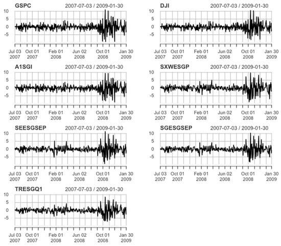
Figure 1.
The rates of return 3 July 2007–30 January 2009.
At the same time, the distribution of the returns has tails, which are heavier than the tails of the normal distribution. To confirm this, we used the Jarque–Bera test and Q-Q plots.
Generally, the daily returns for both types of indices exhibit no significant auto-correlation, supporting the hypothesis that the returns are uncorrelated across time. To confirm this, we applied the Ljung–Box test. Finally, we checked whether the rates of return are characterized by the ARCH effect using the McLeoda and Li test. The null hypothesis is that the rates of return do not have the ARCH effect, while the alternative hypothesis is that they have the ARCH effect. In all subperiods, the ARCH effect was detected in the returns.
In the case of the standardized innovations from the ARMA-GARCH models, at the assumed 5% level of significance, the p-values for the Engle test are greater than 0.05 (see Table A3, Table A4 and Table A5), which means that the null hypothesis was not rejected, i.e., the ARCH effect is not present in the innovations. Hence, the models are free from conditional heteroskedasticity in almost all cases (only in the first period for three indices the ARCH effect is present—Table A2). To verify the autocorrelation in the innovations, we used the Ljung–Box test. The null hypothesis that the innovations are independently distributed was not rejected in all the cases (see Table A2, Table A3, Table A4 and Table A5). It means that the models have been well-chosen and fitted.
Finally, the persistence parameters are close to one, which is high (see Table A2, Table A3, Table A4 and Table A5), meaning that the variance moves slowly through time.
We employ not only normally distributed innovations, but also the Student’s t-distributions, the generalized error distribution (GED) and a skewed version of both. The reason for considering distributions other than normal is that a GARCH model with conditional normal errors has fatter tails than the normal distribution, and for many financial time series the standardized innovations still appear to be leptokurtic. Therefore, assuming a leptokurtic unconditional distribution for the innovations seems more appropriate.
Because the market returns are not normally distributed, the Gaussian copula would not capture tail dependence. Therefore, we fitted the Student’s t-copula and the combination of Clayton and Gumbel copulas. At a 1% significance level for the chosen copulas, we cannot reject the null hypothesis (GoF test), i.e., our copulas are the true copulas. Due to the observed nonnormality in the returns distribution, we measured the dependence by using Kendall’s τ coefficient. All results for the Kendall’s τ coefficient are statistically significant. In the first two subperiods, dependencies were higher than in the next two subperiods (see Table 2, Table 3, Table 5, Table 6, Table 8, Table 9, Table 11 and Table 12). To quantify the degree of tail dependence in each pair, the Kendall’s τ is estimated and the p-values of the independence test based on the Kendall’s τ are determined (see Figure 2 and Table 2 and Table 3). The results indicate the existence of positive, significant dependence.
Table 2.
Dependence structure for the GSPC and ESG indices, 3 July 2007–30 January 2009.
Table 3.
Dependence structure for DJI and ESG indices, 3 July 2007–30 January 2009.
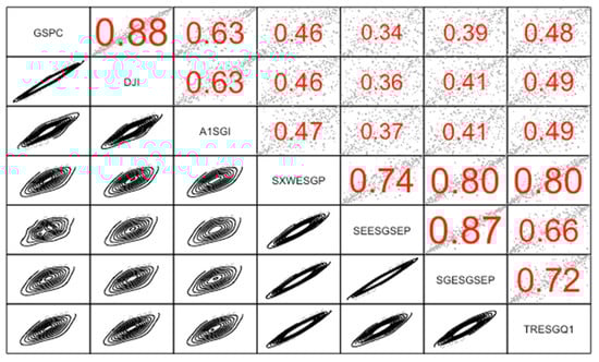
Figure 2.
Kendall’s τ and copulas 3 July 2007–30 January 2009.
We analyzed the dependence for 10 pairs of indices, namely S&P and ESG—5 pairs and DJI and ESG—5 pairs. Dependence between S&P and DJI exhibited lower tail dependence in three subperiods; only in the 2008 global financial crisis was the tail dependence symmetric. In the first and last subperiod, ESG and conventional investments showed lower and symmetric tail dependence—in the first subperiod for 5 pairs in the lower tail, for 5 pairs symmetric; in the third subperiod for 3 pairs in the lower tail and for 7 pairs symmetric. In the second period, ESG and conventional investments exhibited lower and upper tail dependence—for 6 pairs in the lower tail, for 3 pairs symmetric (see Table 2, Table 3, Table 5, Table 6, Table 8, Table 9, Table 11 and Table 12).
3.2. The Global Financial Crisis Period (3 July 2007–30 January 2009)
In the global financial crisis period, all indices are not normally distributed (high kurtosis, mostly positive asymmetry, as confirmed by the Jarque–Bera test) with negative means and similar standard deviations (lower only for SGESGSEP and TRESQ1—Table 1). The year 2008 was characterized by high volatility. Volatility clustering was observed for all indices (Figure 1). There is no consensus in modeling the volatility of conventional indices. There were APGARCH (innovations with normal distribution—norm) for S&P 500 and EGARCH (innovations with skewed Student’s t-distribution—sstd) for the fitted DJI. For ESG indices, GJR-GARCH (innovations with normal distribution) for A1SGI and for other AVGARCH (innovations with normal distribution) fitted best. From Table A2, we can see that all the parameters have very small p-values, which shows their significance. Persistence ranges from 0.9654 to 0.9818 for S&P 500 and DJI, and from 0.9649 to 0.9730 for ESG indices, indicating the slow movement of variance through time.
The highest values of Kendall’s tau (see Figure 2) are between indices of the same type (S&P 500 and DJI, and SEESGSEP and SGESGSEP). High dependence is observed between S&P 500 and A1SGI and between DJI and A1SGI, low dependence between S&P 500 and SEESGSEP and between DJI and SEESGSEP. For example, for the GSPC–SEESGSEP relationship—the observed copula has the lowest dependency—depends by 34.24% on the upper and lower tail (Student’s t-copula was employed). The GSPC–SXWESGP relationship has a dependency of 47.54% on the upper tail, and of 54.41% on the lower tail. It means the interaction has a greater effect in the lower tail (also for GSPC–SGESGSEP, GSPC–TRESGQ1, DJI–SXWESGP, DJI–SGESGSEP, DJI–TRESGQ1).
The dependence between the S&P 500 and ESG indices and between the DJI and ESG indices is modeled by Student’s t and the Joe–Clayton copula (see Table 2 and Table 3). There is one difference—the dependence between S&P 500 and SGESGSEP is described by the Joe–Clayton copula; between DJI and SGESGSEP by the t copula.
3.3. The Period of Debt Crisis in EU (2 December 2009–30 July 2014)
In the period of debt crisis in the EU, all indices are not normally distributed (mostly high kurtosis, negative asymmetry, as confirmed by the Jarque–Bera test) with positive means and similar standard deviations (lower only for DJI and A1SGI—Table 4). Two periods were characterized by high volatility (visible volatility clustering at all indices in 2009 and 2011—Figure 3). To model the volatility of conventional indices ARMA-EGARCH models (with innovations with skewed GED—sged) were fitted. In the case of ESG indices ARMA-EGARCH models also fitted best, but different distributions for innovation were applied (mostly skewed Student’s t-distribution and skewed GED for SEESGSEP). From Table A3 we can see that all the parameters have very small p-values, which shows their statistical significance. Persistence for S&P 500 and DJI is similar (0.9410–0.9411) for ESG indices ranges from 0.9594 to 0.9910, indicating slow movement of variance through time.
Table 4.
Descriptive statistics, 2 December 2009–30 July 2014.
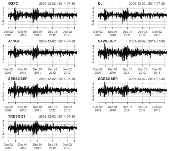
Figure 3.
The rates of return, 2 December 2009–30 July 2014.
The highest values of Kendall’s τ (see Figure 4) are between indices of the same type (S&P 500 and DJI, and SEESGSEP and SGESGSEP). High dependence is observed between S&P 500 and A1SGI and between DJI and A1SGI; low dependence between S&P 500 and SEESGSEP and between DJI and SEESGSEP. For example, for the GSPC–SEESGSEP relationship—the observed copula has the lowest dependency (but higher comparing to previous period)—depends by 52.82% on the upper tail and 50.95% on the lower tail. The GSPC-A1SGI relationship has a dependency of 84.33% on the upper tail, and of 89.85% on the lower tail. It means the interaction has a greater effect in the upper tail for the first pair and for DJI–SEESGSEP, DJI–SGESGSEP, and GSPC–SGESGSEP. The greater effect in the lower tail is observed for the second pair and for the other indices.
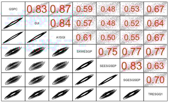
Figure 4.
Kendall’s τ and copulas, 2 December 2009–30 July 2014.
The dependence between the S&P 500 and ESG indices and between the DJI and ESG indices is modeled by the Clayton–Gumbel and Joe–Clayton copulas (see Table 5 and Table 6). The dependences between S&P 500 and SXWESGP, SGESGSEP, and TRESGQ1 comparing to DJI’s dependence were modeled differently. For example, GSPC–SGESGSEP relationship is modeled by the Clayton–Gumbel copula, and DJI–SGESGSEP by the Joe–Clayton copula.
Table 5.
Dependence structure for GSPC and ESG indices, 2 December 2009–30 July 2014.
Table 6.
Dependence structure for DJI and ESG indices, 2 December 2009–30 July 2014.
3.4. The Russian Financial Crises, Fall in Oil Prices (3 June 2014–31 January 2017)
In the Russian financial crises and fall in oil prices period, all indices are not normally distributed (mostly high kurtosis, negative asymmetry, as confirmed by the Jarque–Bera test) with mostly positive means (for three ESG indices the mean was negative) and similar standard deviations for S&P 500 and DJI. In the case of standard deviation for the ESG indices, large differences were observed—low for A1SGI and high for SEESGSEP (Table 7). In this period, three subperiods characterized by high volatility (visible volatility clustering of all indices in 2015 and the beginning of 2016, and a large drop in the middle of 2016—Figure 5) were present. The volatility of three indices, namely S&P 500, DJI and A1SGI, was modeled by AVGARCH (innovations with skewed Student’s t-distribution). There is no consensus in the modeling volatility of the ESG indices. GARCH, EGARCH, and AVGARCH (innovations with Student’s t-distribution in all models) were applied. From Table A4, we can see that all the parameters have very small p-values, which shows their statistical significance. Persistence ranges from 0.9655 to 0.9749 for S&P 500 and DJI, and from 0.8972 to 0.9716 for ESG indices.
Table 7.
Descriptive statistics, 3 June 2014–31 January 2017.
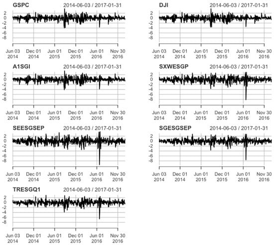
Figure 5.
The rates of return, 3 June 2014–31 January 2017.
The highest values of Kendall’s τ (see Figure 6) are between indices of the same type (S&P 500 and DJI, and SEESGSEP and SGESGSEP). High dependence is observed between S&P 500 and A1SGI and between DJI and A1SGI; low dependence between S&P 500 and SEESGSEP and between DJI and SEESGSEP. For example, for the DJI–SEESGSEP relationship—the observed copula has the lowest dependency (lower compared to previous periods too)—depends by 21.90% on the upper tail and 21.90% on the lower tail. The GSPC–A1SGI relationship has a dependency of 85.21% on the upper tail, and of 85.21% on the lower tail. It means that the interaction has the same effect in the upper tail and in the lower tail. The greater effects in the lower tail are observed for GSPC–TRESGQ1, DJI–TRESGQ1 and DJI–A1SGI.
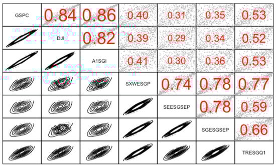
Figure 6.
Kendall’s τ and copulas, 3 June 2014–31 January 2017.
The dependences between the S&P 500 and ESG indices and between the DJI and ESG indices were modeled by the Clayton–Gumbel and t copulas (see Table 8 and Table 9). The dependence between S&P 500 and A1SGI compared to the DJI dependence was modeled differently. For example, the GSPC–A1SGI relationship is modeled by Student’s t copula, and DJI–GESGSEP by Clayton–Gumbel copula.
Table 8.
Dependence structure for the GSPC and ESG indices, 3 June 2014–31 January 2017.
Table 9.
Dependence structure for DJI and ESG indices, 3 June 2014–31 January 2017.
3.5. The Stabilization Period (4 January 2017–31 December 2019)
In the stabilization period, all indices are not normally distributed (mostly low kurtosis comparing to previous periods, but higher than for normal distribution, negative asymmetry, as confirmed by the Jarque–Bera test) with positive means and similar standard deviations for S&P 500, DJI, and A1SGI. In the case of standard deviation for other ESG indices, large differences were observed—low for SGESGSEP and high for SEESGSEP (Table 10). In the whole period, two subperiods characterized by high volatility (visible volatility clustering in beginning of 2018 and the beginning of 2019—Figure 7) were observed for S&P 500, DJI, and A1SGI. For other ESG indices not only these clusters were observed (high volatility was during the whole of 2018 and the first half of 2019). Volatility of three indices, namely S&P 500, DJI, and A1SGI, was modeled by AVGARCH (innovations with skewed Student’s t and skewed GED distributions). There is no consensus in the modeling volatility of the ESG indices. There were applied GJR-GARCH and EGARCH (innovations with Student’s t and skewed normal distributions). From Table A5, we can see that all the parameters have very small p-values, which shows their statistical significance. Persistence ranges from 0.9581 to 0.9564 for S&P 500 and DJI, and from 0.9169 to 0.9628 for the ESG indices.
Table 10.
Descriptive statistics, 4 January 2017–31 December 2019.
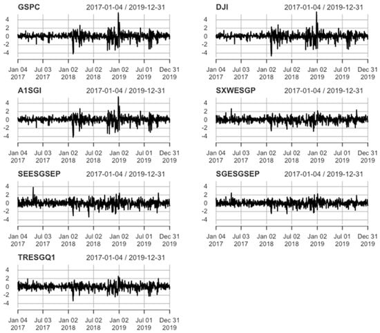
Figure 7.
The rates of return, 4 January 2017–31 December 2019.
The highest values of Kendall’s τ (see Figure 8) are between indices of the same type (S&P 500 and DJI, and SEESGSEP and SGESGSEP). High dependence is observed between S&P 500 and A1SGI and between DJI and A1SGI, low dependence between S&P 500 and SEESGSEP, and between DJI and SEESGSEP. For example, for the GSPC–SEESGSEP relationship—the observed copula has the lowest dependency—depends by 16.50% on the upper tail and 16.50% on the lower tail (the same dependency). The pair GSPC–A1SGI has a dependency of 88.22% on the lower tail, and of 85.32% on the upper tail. It means the interaction has a greater effect in the lower tail. This interaction was also observed in the pairs DJI–A1SGI, DJI–TRESGQ1, DJI–SXWESGP, and GSPC–TRESGQ1.
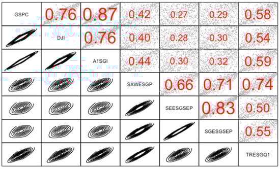
Figure 8.
Kendall’s τ and copulas, 4 January 2017–31 December 2019.
The dependences between the S&P 500 and ESG indices and between the DJI and ESG indices were modeled by the Clayton–Gumbel, t, and Joe–Clayton copula (see Table 11 and Table 12). Dependences between S&P 500 and SEESGSEP, and between S&P 500 and SGESGSEP compared to DJI were modeled by using the t copula. In the other cases, we used other copulas. For example, the GSPC-TRESGQ1 relationship is modeled by the Clayton–Gumbel copula, and DJI–SGESGSEP by the Survival Joe–Clayton copula.
Table 11.
Dependence structure for the GSPC and ESG indices, 4 January 2017–31 December 2019.
Table 12.
Dependence structure for the DJI and ESG indices, 4 January 2017–31 December 2019.
4. Discussion
Our study does not confirm the outperformance of the ESG indices compared to conventional ones in terms of risk in the considered subperiods. However, generalization of the results is limited by the selection of a market index as a proxy of an investment portfolio. Other empirical studies demonstrate a strong correlation between the lower risk related to sustainability and better financial performance (Whelan et al. 2021). During the 2008 global financial crisis Fernández et al. (2019) found that German green mutual funds had risk-adjusted returns slightly better than their peers (in the noncrisis period, they were equal to conventional funds but better than the SRI funds). Similarly, ESG stock indices performed better and recovered faster after the 2008 global financial crisis (Wu et al. 2017). Other results confirm these findings, as in economic downturns, the high-rated mutual funds outperformed the low-rated funds, based on the Sharpe ratio (Das et al. 2018a, 2018b; Khajenouri and Schmidt 2020). In line are research by Abate et al. (2021) that mutual funds investing in high ESG stocks perform better than investing in low ESG score stocks. Gil-Bazo et al. (2010) confirm that SRI funds perform better than their conventional counterparts.
In the study we evaluate whether conventional stock portfolios, including ESG companies, can effectively decrease portfolio risk, especially in times of financial distress on the market. Generally, we observe in all subperiods almost-weak to high lower-tail dependence between the ESG and conventional indices. Our findings indicate that there is low or symmetric tail dependence between ESG and conventional indices, meaning that if the ESG index decreases, the conventional one will also decrease accordingly. In the two first subperiods (economic downturn periods) lower tail dependence coefficients are higher comparing to the next two periods (‘stabilization’ periods). We conclude that dependencies exist, can be quantified, and are not negligible, especially in times of crisis.
In risk management of an asset portfolio, we are interested whether the decline of one (or more) assets may influence the behavior of the other assets in a portfolio. Especially, the occurrence of simultaneous extreme events on the market implies that risk diversification breaks down just when it is crucial. In case of extreme events, classical dependence analysis (e.g., linear correlation) fails, a copula approach is used. Some researchers argue that considering ESG practices when creating an equity portfolio (selecting companies with high ESG scores) can act as protection against left-tail risk; therefore, reducing ex-ante expectations of a left-tail event (Shafer and Szado 2020; De and Clayman 2015; Djoutsa Wamba et al. 2020).
The measurement of the tail dependence between ESG and conventional investment based on the copula approach, allows to monitor extreme risks between them. Understanding dependencies and risks is important for setting up adequate risk management as well as construction portfolios—ESG-diversified and resilient to crises. Bax et al. (2021) use the R-vine copula ESG risk model. They estimate all the conditional dependencies among assets as well as specify their interactions as modeled by different copulas families, but they also introduce three ESG risk measures that capture ESG risk, market risk conditionally on the ESG class, as well as an idiosyncratic risk component.
5. Conclusions
As interest in ESG investments grows, it is crucial to better understand the various risks and return tradeoffs between ESG and conventional stocks and the dependence structures between them. We used GARCH family models to estimate conditional volatilities and the copula approach, in particular the (tail) dependence structure between ESG and conventional investments to quantify the overall and lower tail risk between these two investments.
Hypothesis 1, that ESG investments outperform conventional ones in terms of risk was negatively verified—there are indices that underperform the conventional indices in selected subperiods. Hypothesis 2, that asymptotic dependence increases during the crisis on the market (declines of stock market indices), and it stabilizes during non-crisis periods was positively verified.
The findings indicate that there is no significant difference in daily returns of ESG indices and conventional ones.
The parameters are significant among all the estimations and comparisons, showing that GARCH family models may appropriately model the ESG and conventional index data. In most subperiods, the data for the ESG and conventional indices were negatively skewed. The EGARCH models this type of behavior, but in this study, also AVGARCH model was applied. Surprisingly, GJR-GARCH was not often used.
We found relations between the selected ESG indices. A1GSI is related in construction to S&P 500, while three other ESG indices—SXWESGP, SEESGSEP, and SGESGSEP are related to each other. These relations were visible in similar behavior of the rates of return. Volatility clustering observed at S&P 500, DJI, and A1SGI was different from that in other ESG indices (but the scale of these differences depends on the subperiod). In the first subperiod, one cluster was observed for all the indices (there is no difference visible). In the second and third subperiod, two clusters were found for all indices, but the difference between these two groups of indices was present. The most visible differences were observed in the last subperiod. Only in the second period, results of model estimation are consistent for all the indices (ARMA-EGARCH models with innovations sged and sstd).
We cannot confirm that the volatility of conventional indices should be modeled using different models than the volatility of the ESG—this depends on the time period and the market events. There are periods when volatility of all the indices may be modeled by using the same models, when there is a difference between the modeling of conventional and ESG indices, and when there is a difference between the modeling of ESG indices.
The characteristics of the time series indicated the need to apply to the dependence analysis copula approach. To capture tail dependence, Student’s t-copula and the combination of the Clayton and Gumbel copulas were fitted best in this study. The choice of an appropriate copula function is crucial. Two features are important regarding the copula selection. The general structure of the chosen copula should coincide with the dependence structure of the real data. If the data show tail dependence than we must apply a copula which comprises tail dependence.
In the periods of economic downturn (declines of stock market indices), the dependencies measured by Kendell’s tau coefficients were higher than in the less turbulent periods.
The lower tail dependence and symmetric dependence between ESG and conventional investments were detected. High values of low tail-dependence coefficients were observed in the economic downturn periods; low in stabilization periods. This signifies higher dependence of extreme values in the economic downturn periods and low dependence of extreme values in stabilization periods.
We conclude that when selecting the right model, the preliminary analysis of data is necessary, and the selection of the volatility model should be carried out for subperiods regarding different market-event characteristics. Results show, as in cases of systemic risk, that analysis of volatility and dependence structure should be carried out separately—in the periods of economic downturn and in less turbulent times.
To extend this research for the future, a more detailed analysis, including ESG and non-ESG companies from different markets (developed and developing) would be beneficial. In addition, application of a time-varying model (time-varying copula) would give insights into dependence structure.
Author Contributions
Conceptualization, K.K.; methodology, K.K. and J.G.; software, J.G.; formal analysis, K.K. and J.G.; investigation, K.K. and J.G.; data curation, J.G.; writing—original draft preparation, K.K. and J.G.; writing—review and editing, K.K. and J.G.; visualization, K.K. and J.G.; supervision, K.K.; funding acquisition, K.K. All authors have read and agreed to the published version of the manuscript.
Funding
This research was funded by Wroclaw University of Economics and Business.
Conflicts of Interest
The authors declare no conflict of interest.
Appendix A
Table A1.
Description of ESG indices.
Table A1.
Description of ESG indices.
| Name | Ticker | Description | Market |
|---|---|---|---|
| STOXX GLOBAL ESG LEADERS Index | .SXWESGP | The index offers a representation of the leading global companies in terms of environmental, Social, and governance criteria, based on ESG indicators provided by Sustainalytics | Global |
| STOXX Europe ESG Leaders Select 30 Price EUR Index | .SEESGSEP | The index captures the performance of stocks with low volatility and high dividends from the STOXX Global ESG Leaders Index. | Europe |
| STOXX Global ESG Leaders Select 50 Price EUR Index | .SGESGSEP | The index captures the performance of stocks with low volatility and high dividends from the STOXX Global ESG Leaders Index. The component selection process first excludes all stocks whose 3- or 12-month historical volatilities are the highest. Among the remaining stocks, the 50 stocks with the highest 12-month historical dividend yields are selected to be included in the index. | Global |
| Refinitiv IX Global ESG Equal Weighted Price Only | .TRESGQ1 | The index is a benchmark for investors seeking companies that actively invest in and promote ESG values and principles. The index tracks the price return and net total return of publicly traded equities across the world that display relatively high ESG. The constituents’ universe is derived from Refinitiv Global Developed Index (the parent index). | Global |
| Dow Jones Sustainability North America Composite Index | .A1SGI | The index comprises North American sustainability leaders as identified by S&P Global through the Corporate Sustainability Assessment (CSA). It represents the top 20% of the largest 600 North American companies in the S&P Global BMI based on long-term ESG criteria. | North America |
Source: own elaboration based on particular indices’ websites.
Appendix B
Table A2.
Family ARMA-GARCH models, 3 July 2007–30 January 2009.
Table A2.
Family ARMA-GARCH models, 3 July 2007–30 January 2009.
| GSPC | DJI | A1SGI | SXWESGP | SEESGSEP | SGESGSEP | TRESGQ1 | |
|---|---|---|---|---|---|---|---|
| Model | APARCH | EGARCH | GJR GARCH | AVGARCH | AVGARCH | AVGARCH | AVGARCH |
| Distribution | norm | sstd | norm | norm | norm | norm | norm |
| −1.8549 | −1.8857 | −1.8615 | −0.2658 | ||||
| 0.0000 | 0.0000 | 0.0000 | 0.0000 | ||||
| −0.9319 | −0.9614 | −0.8876 | −1.0050 | ||||
| 0.0000 | 0.0000 | 0.0000 | 0.0000 | ||||
| 1.7806 | 1.8063 | 1.6787 | 0.2702 | 0.1156 | |||
| 0.0000 | 0.0000 | 0.0000 | 0.0000 | 0.0167 | |||
| 0.6639 | 0.7189 | 0.3917 | 1.0118 | −0.0562 | |||
| 0.0000 | 0.0000 | 0.0000 | 0.0000 | 0.0285 | |||
| −0.2059 | −0.1801 | −0.3394 | |||||
| 0.0000 | 0.0000 | 0.0000 | |||||
| 0.0512 | 0.0001 | 0.0555 | 0.0370 | 0.0454 | 0.0382 | 0.0312 | |
| 0.0000 | 0.9834 | 0.0000 | 0.0000 | 0.0000 | 0.0000 | 0.0000 | |
| 0.0000 | −0.1579 | 0.0000 | 0.0926 | 0.1398 | 0.1164 | 0.0753 | |
| 1.0000 | 0.0000 | 1.0000 | 0.0000 | 0.0000 | 0.0000 | 0.0000 | |
| 0.1068 | |||||||
| 0.0000 | |||||||
| 0.8751 | 0.9818 | 0.8774 | 0.8314 | 0.7855 | 0.8196 | 0.8354 | |
| 0.0000 | 0.0000 | 0.0000 | 0.0000 | 0.0000 | 0.0000 | 0.0000 | |
| −0.4094 | 0.1037 | 0.1778 | |||||
| 0.9532 | 0.0000 | 0.0001 | |||||
| 1.0000 | |||||||
| 0.0000 | |||||||
| 0.4877 | 0.4084 | 0.5056 | 0.6569 | ||||
| 0.0000 | 0.0000 | 0.0000 | 0.0000 | ||||
| 0.8895 | 0.7126 | 0.6472 | 0.9940 | ||||
| 0.0000 | 0.0000 | 0.0000 | 0.0000 | ||||
| 1.0751 | |||||||
| 0.0000 | |||||||
| skew | 0.8852 | ||||||
| 0.0000 | |||||||
| shape | 11.4791 | ||||||
| 0.0642 | |||||||
| Akaike | 3.8296 | 3.7112 | 3.6759 | 3.7624 | 3.6824 | 3.6065 | 3.5371 |
| Bayes | 3.9521 | 3.8235 | 3.7678 | 3.8135 | 3.7743 | 3.6576 | 3.6085 |
| Ljung–Box test | 4.4482 | 6.3567 | 9.9787 | 6.9881 | 5.9840 | 6.6419 | 7.7529 |
| 0.9249 | 0.7845 | 0.4424 | 0.7266 | 0.8166 | 0.7588 | 0.6530 | |
| Engle Arch test | 8.6312 | 15.2820 | 12.3802 | 21.5479 | 16.7602 | 30.0986 | 24.3912 |
| 0.7341 | 0.2264 | 0.4156 | 0.0429 | 0.1588 | 0.0027 | 0.0180 | |
| Persistence | 0.9654 | 0.9818 | 0.9663 | 0.9730 | 0.9649 | 0.9693 | 0.9721 |
Note: the first row indicates the estimate parameters (or test statistics) and the second row—the p-value of the Student’s t-test (or appropriate test); Ljung–Box and Engle ARCH tests were calculated for standardized innovations.
Table A3.
ARMA-EGARCH models, 2 December 2009–30 July 2014.
Table A3.
ARMA-EGARCH models, 2 December 2009–30 July 2014.
| GSPC | DJI | A1SGI | SXWESGP | SEESGSEP | SGESGSEP | TRESGQ1 | |
|---|---|---|---|---|---|---|---|
| Distribution | sged | sged | sstd | sstd | sged | sstd | sstd |
| −0.5969 | −0.2909 | 0.0773 | |||||
| 0.0000 | 0.0000 | 0.0000 | |||||
| 0.5690 | 0.2501 | ||||||
| 0.0000 | 0.0000 | ||||||
| −0.0042 | −0.0162 | −0.0081 | 0.0027 | 0.0023 | −0.0017 | 0.0024 | |
| 0.4793 | 0.0005 | 0.1138 | 0.1199 | 0.2122 | 0.6040 | 0.3074 | |
| −0.3983 | −0.3570 | −0.3832 | −0.1023 | −0.0918 | −0.1150 | −0.1117 | |
| 0.0000 | 0.0000 | 0.0000 | 0.0000 | 0.0000 | 0.0000 | 0.0000 | |
| 0.1515 | 0.1371 | 0.1687 | |||||
| 0.0000 | 0.0049 | 0.0000 | |||||
| 0.9410 | 0.9411 | 0.9594 | 0.9910 | 0.9867 | 0.9816 | 0.9867 | |
| 0.0000 | 0.0000 | 0.0000 | 0.0000 | 0.0000 | 0.0000 | 0.0000 | |
| −0.1456 | −0.0852 | −0.1791 | 0.0668 | 0.0672 | 0.1182 | 0.0808 | |
| 0.0323 | 0.0003 | 0.0126 | 0.0000 | 0.0000 | 0.0002 | 0.0019 | |
| 0.2681 | 0.2472 | 0.2805 | |||||
| 0.0001 | 0.0003 | 0.0001 | |||||
| skew | 0.8098 | 0.8356 | 0.7841 | 0.8657 | 0.8563 | 0.8689 | 0.8251 |
| 0.0000 | 0.0000 | 0.0000 | 0.0000 | 0.0000 | 0.0000 | 0.0000 | |
| shape | 1.3919 | 1.4247 | 7.7845 | 8.1811 | 1.5014 | 8.8081 | 6.7950 |
| 0.0000 | 0.0000 | 0.0000 | 0.0000 | 0.0000 | 0.0001 | 0.0000 | |
| Akaike | 2.4940 | 2.3325 | 2.3731 | 2.9187 | 2.8993 | 2.5299 | 2.6496 |
| Bayes | 2.5382 | 2.3767 | 2.4084 | 2.9496 | 2.9258 | 2.5564 | 2.6762 |
| Ljung–Box test | 7.6686 | 4.6382 | 6.8038 | 5.5808 | 4.8186 | 6.0897 | 7.1695 |
| 0.6612 | 0.9140 | 0.7438 | 0.8492 | 0.9030 | 0.8077 | 0.7094 | |
| Engle ARCH test | 7.8238 | 6.3159 | 7.2004 | 8.4786 | 13.9807 | 17.9072 | 10.1396 |
| 0.7987 | 0.8993 | 0.8441 | 0.7467 | 0.3019 | 0.1185 | 0.6037 | |
| Persistence | 0.9410 | 0.9411 | 0.9594 | 0.9910 | 0.9867 | 0.9816 | 0.9867 |
Note: the first row indicates the estimate parameters (or test statistics) and the second row—the p-value of the Student’s t-test (or appropriate test); Ljung–Box and Engle ARCH tests were calculated for standardized innovations.
Table A4.
Family GARCH models, 3 June 2014–31 January 2017.
Table A4.
Family GARCH models, 3 June 2014–31 January 2017.
| GSPC | DJI | A1SGI | SXWESGP | SEESGSEP | SGESGSEP | TRESGQ1 | |
|---|---|---|---|---|---|---|---|
| Model | AVGARCH | AVGARCH | AVGARCH | EGARCH | EGARCH | GARCH | AVGARCH |
| Distribution | sstd | sstd | sstd | std | std | std | std |
| 0.0361 | 0.0285 | 0.0302 | −0.0215 | −0.0147 | 0.0723 | 0.0326 | |
| 0.0000 | 0.0000 | 0.0000 | 0.0560 | 0.2977 | 0.0052 | 0.0007 | |
| 0.2033 | 0.2302 | 0.2782 | −0.1276 | −0.1335 | 0.1981 | 0.1807 | |
| 0.0000 | 0.0000 | 0.0000 | 0.0001 | 0.0007 | 0.0000 | 0.0000 | |
| 0.6804 | 0.7186 | 0.7042 | 0.9419 | 0.8972 | 0.7133 | 0.7933 | |
| 0.0000 | 0.0000 | 0.0000 | 0.0000 | 0.0000 | 0.0000 | 0.0000 | |
| 0.2418 | 0.2775 | ||||||
| 0.0002 | 0.0003 | ||||||
| 0.1086 | −0.1145 | −0.2498 | −0.1651 | ||||
| 0.1826 | 0.0000 | 0.0000 | 0.0450 | ||||
| 1.1870 | 1.1419 | 1.1495 | 0.9274 | ||||
| 0.0000 | 0.0000 | 0.0000 | 0.0000 | ||||
| skew | 0.8196 | 0.8599 | 0.8440 | ||||
| 0.0000 | 0.0000 | 0.0000 | |||||
| shape | 11.2696 | 7.7111 | 11.4148 | 10.6788 | 8.5965 | 9.6351 | 7.6282 |
| 0.0084 | 0.0001 | 0.0037 | 0.0022 | 0.0003 | 0.0018 | 0.0001 | |
| Akaike | 2.1554 | 2.1590 | 2.1985 | 2.5601 | 2.7756 | 2.4024 | 2.3052 |
| Bayes | 2.2029 | 2.2065 | 2.2460 | 2.5940 | 2.8096 | 2.4296 | 2.3458 |
| Ljung–Box test | 15.6265 | 12.3524 | 13.1544 | 11.6801 | 7.0749 | 13.3207 | 11.0541 |
| 0.1108 | 0.2622 | 0.2152 | 0.3070 | 0.7184 | 0.2063 | 0.3533 | |
| Engle ARCH test | 5.3622 | 4.8535 | 8.7917 | 9.6174 | 9.4367 | 12.2077 | 12.4372 |
| 0.9448 | 0.9627 | 0.7206 | 0.6495 | 0.6653 | 0.4291 | 0.4112 | |
| Persistence | 0.9655 | 0.9749 | 0.9716 | 0.9419 | 0.8972 | 0.9114 | 0.9668 |
Note: the first row indicates the estimate parameters (or test statistics) and the second row—the p-value of the Student’s t-test (or appropriate test); Ljung–Box and Engle ARCH tests were calculated for standardized innovations.
Table A5.
Family ARMA-GARCH models, 4 January 2017–31 December 2019.
Table A5.
Family ARMA-GARCH models, 4 January 2017–31 December 2019.
| GSPC | DJI | A1SGI | SXWESGP | SEESGSEP | SGESGSEP | TRESGQ1 | |
|---|---|---|---|---|---|---|---|
| Model | AVGARCH | AVGARCH | AVGARCH | EGARCH | EGARCH | GJR GARCH | EGARCH |
| Distribution | sged | sstd | sged | std | std | std | snorm |
| 0.0766 | |||||||
| 0.0462 | |||||||
| 0.0392 | 0.0406 | 0.0338 | −0.0707 | −0.0417 | 0.0208 | −0.0443 | |
| 0.0000 | 0.0000 | 0.0000 | 0.0141 | 0.0407 | 0.0207 | 0.0021 | |
| 0.1456 | 0.1065 | 0.1321 | −0.1286 | −0.0982 | 0.0067 | −0.1526 | |
| 0.0000 | 0.0000 | 0.0000 | 0.0000 | 0.0036 | 0.7335 | 0.0000 | |
| 0.7806 | 0.8708 | 0.7995 | 0.9169 | 0.9394 | 0.8845 | 0.9402 | |
| 0.0000 | 0.0000 | 0.0000 | 0.0000 | 0.0000 | 0.0000 | 0.0000 | |
| 0.1402 | 0.1375 | 0.1149 | 0.1793 | ||||
| 0.0077 | 0.0009 | 0.0078 | 0.0000 | ||||
| 0.5809 | 1.0000 | 0.4573 | |||||
| 0.0000 | 0.0001 | 0.0000 | |||||
| 0.5806 | 0.0786 | 0.6727 | |||||
| 0.0000 | 0.0695 | 0.0000 | |||||
| skew | 0.8846 | 0.8334 | 0.8564 | 0.8620 | |||
| 0.0000 | 0.0000 | 0.0000 | 0.0000 | ||||
| shape | 1.2853 | 4.6528 | 1.3843 | 14.0514 | 8.7823 | 12.4842 | |
| 0.0000 | 0.0000 | 0.0000 | 0.0145 | 0.0002 | 0.0122 | ||
| Akaike | 1.8836 | 1.9762 | 1.9035 | 1.9509 | 2.1482 | 1.8526 | 1.9036 |
| Bayes | 1.9269 | 2.0195 | 1.9468 | 1.9880 | 2.1791 | 1.8835 | 1.9345 |
| Ljung–Box test | 8.6446 | 7.6484 | 9.9759 | 9.0690 | 12.1615 | 9.3624 | 10.8849 |
| 0.5661 | 0.6631 | 0.4426 | 0.5256 | 0.2744 | 0.4981 | 0.3666 | |
| Engle ARCH test | 9.3952 | 12.5922 | 10.9797 | 10.0092 | 20.3661 | 14.3953 | 8.8700 |
| 0.6689 | 0.3994 | 0.5307 | 0.6151 | 0.0605 | 0.2762 | 0.7140 | |
| Persistence | 0.9581 | 0.9564 | 0.9628 | 0.9169 | 0.9394 | 0.9487 | 0.9402 |
Note: the first row indicates the estimate parameters (or test statistics) and the second row—the p-value of the Student’s t-test (or appropriate test); Ljung–Box and Engle ARCH tests were calculated for standardized innovations.
References
- Abate, Guido, Ignazio Basile, and Pierpaolo Ferrari. 2021. The level of sustainability and mutual fund performance in europe: An empirical analysis using ESG ratings. Corporate Social Responsibility and Environmental Management 28: 1446–55. [Google Scholar] [CrossRef]
- Ang, Andrew, and Geert Bekaert. 2002. International asset allocation with regime shifts. Review of Financial Studies 15: 1137–87. [Google Scholar] [CrossRef]
- Apergis, Nicholas, Vassilios Babalos, Christina Christou, and Rangan Gupta. 2015. Identifying Asymmetries between Socially Responsible and Conventional Investments. Working Papers: 2015-37. Pretoria: Department of Economics, University of Pretoria. [Google Scholar]
- Bax, Karoline, Özge Sahin, Claudia Czado, and Sandra Paterlini. 2021. ESG, Risk, and (Tail) Dependence. SSRN Electronic Journal. [Google Scholar] [CrossRef]
- Bollerslev, Tim. 1986. Generalized autoregressive conditional heteroscedasticity. Journal of Econometrics 31: 307–27. [Google Scholar] [CrossRef]
- Box, George E. P., and Gwilym M. Jenkins. 1983. Analiza Szeregów Czasowych. Warszawa: Wydawnictwo PWN. [Google Scholar]
- Brockwell, Peter J., and Richard A. Davis. 1991. Time Series: Theory and Methods. New York: Springer. [Google Scholar] [CrossRef]
- Charles, Amélie, Olivier Darné, and Jessica Fouilloux. 2016. The Impact of Screening Strategies on the Performance of ESG Indices. July 12. Available online: https://hal.archives-ouvertes.fr/hal-01344699 (accessed on 1 October 2021).
- Das, Nandita, Bernadette Ruf, Swarn Chatterjee, and Aman Sunder. 2018a. Fund characteristics and performances of socially responsible mutual funds: Do ESG ratings play a role? Journal of Accounting and Finance 18: 57–69. [Google Scholar] [CrossRef]
- Das, Nandita, Swarn Chatterje, Bernadette Ruf, and Aman Sunder. 2018b. ESG ratings and the performance of socially responsible mutual funds: A panel study journal of finance issues esg ratings and the performance of socially responsible mutual funds: A panel study. Journal of Finance Issues 17: 49–57. [Google Scholar]
- De, Indrani, and Michelle R. Clayman. 2015. The benefits of socially responsible investing: An active manager’s perspective. The Journal of Investing 24: 49–72. [Google Scholar] [CrossRef]
- Ding, Zhuanxin, Clive William John Granger, and Robert F. Engle. 1993. A long memory property of stock market returns and a new model. Journal of Empirical Finance 1: 83–106. [Google Scholar] [CrossRef]
- Djoutsa Wamba, Léopold, Jean Michel Sahut, Eric Braune, and Frédéric Teulon. 2020. Does the optimization of a company’s environmental performance reduce its systematic risk? New evidence from European listed companies. Corporate Social Responsibility and Environmental Management 27: 1677–94. [Google Scholar] [CrossRef]
- Engle, Robert F. 1982. Autoregressive conditional heteroscedasticity with estimates of the variance of United Kingdom inflation. Econometrica 50: 987–1007. [Google Scholar] [CrossRef]
- Engle, Robert F., and Victor K. Ng. 1993. Measuring and testing the impact of news on volatility. The Journal of Finance 48: 1749–78. [Google Scholar] [CrossRef]
- Fama, Eugene F., and Eugene F. Fama. 1965. The behaviour of stock market prices. Journal of Business 38: 34–105. [Google Scholar] [CrossRef]
- Fernández, Manuel Salazar, Ahmad Abu-Alkheil, and Ghadeer M. Khartabiel. 2019. Do German green mutual funds perform better than their peers. Business and Economics Research Journal 10: 297–312. [Google Scholar] [CrossRef]
- Friede, Gunnar. 2019. Why don’t we see more action? A metasynthesis of the investor impediments to integrate environmental, social, and governance factors. Business Strategy and the Environment 28: 1260–82. [Google Scholar] [CrossRef]
- Genest, Christian, Jean François Quessy, and Bruno Rémillard. 2006. Goodness-of-Fit procedures for copula models based on the probability integral transformation. Scandinavian Journal of Statistics 33: 337–66. [Google Scholar] [CrossRef]
- Giese, Guido, and Linda-Eling Lee. 2019. Weighing the Evidence: ESG and Equity Returns. MSCI Research Insight. Available online: https://www.msci.com/www/research-paper/weighing-the-evidence-esg-and/01315636760 (accessed on 24 October 2021).
- Gil-Bazo, Javier, Pablo Ruiz-Verdú, and André A. P. Santos. 2010. The performance of socially responsible mutual funds: The role of fees and management companies. Journal of Business Ethics 94: 243–63. [Google Scholar] [CrossRef]
- Glosten, Lawrence R., Ravi Jagannathan, and David E. Runkle. 1993. On the relation between expected value and the volatility of the nominal excess return on stocks. Journal of Finance 48: 1779–801. [Google Scholar] [CrossRef]
- HKEX. 2020. Performance of ESG Equity Indices Versus Traditional Equity Indices. Available online: https://www.hkex.com.hk/-/media/HKEX-Market/News/Research-Reports/HKEx-Research-Papers/2020/CCEO_ESGEqIdx_202011_e.pdf (accessed on 24 October 2021).
- Jain, Mansi, Gagan Deep Sharma, and Mrinalini Srivastava. 2019. Can sustainable investment yield better financial returns: A comparative study of ESG indices and MSCI indices. Risks 7: 15. [Google Scholar] [CrossRef]
- Jondeau, Eric. 2016. Asymmetry in Tail Dependence in Equity Portfolios. Computational Statistics and Data Analysis 100: 351–68. [Google Scholar] [CrossRef]
- Khajenouri, Daniel, and Jacob Schmidt. 2020. Standard or sustainable—Which offers better performance for the passive investor. Journal of Applied Finance & Banking 11: 61–71. [Google Scholar] [CrossRef]
- Longin, Franqois, and Bruno Solnik. 2001. Extreme correlation of international equity markets. The Journal of Finance LVI: 649–76. [Google Scholar] [CrossRef]
- Managi, Shunsuke, Tatsuyoshi Okimoto, and Akimi Matsuda. 2012. Do socially responsible investment indexes outperform conventional indexes? Applied Financial Economics 22: 1511–27. [Google Scholar] [CrossRef]
- Mandelbrot, Benoit. 1963. The Variation of Certain Speculative Prices. The Journal of Business 36: 394. [Google Scholar] [CrossRef]
- Markowitz, Harry. 1952. Portfolio Selection. Journal of Finance 7: 77–91. [Google Scholar]
- Messaoud, Samia Ben, and Chaker Aloui. 2015. Measuring risk of Portfolio: GARCH-Copula model. Journal of Economic Integration 30: 172–205. [Google Scholar] [CrossRef]
- Nelsen, Roger B. 2006. An introduction to Copulas. New York: Springer. [Google Scholar] [CrossRef]
- Nelson, Daniel B. 1991. Conditional heteroskedasticity in asset returns: A new approach. Econometrica 59: 347. [Google Scholar] [CrossRef]
- Ortas, Eduardo, José M. Moneva, Roger Burritt, and Joanne Tingey-Holyoak. 2014. Does sustainability investment provide adaptive resilience to ethical investors? evidence from Spain. Journal of Business Ethics 124: 297–309. [Google Scholar] [CrossRef]
- Ouchen, Abdessamad. 2021. Is the ESG Portfolio Less Turbulent than a Market Benchmark Portfolio? Risk Management, 1–33. [Google Scholar] [CrossRef]
- Patton, Andrew J. 2006. Copula-Based Models for Financial Times Series. Working Papers: OMI11/07. Oxford: The Oxford-Man Institute, University of Oxford. [Google Scholar]
- Pedersen, Lasse Heje, Shaun Fitzgibbons, and Lukasz Pomorski. 2021. Responsible investing: The ESG-efficient frontier. Journal of Financial Economics 142: 572–97. [Google Scholar] [CrossRef]
- Plastun, Alex, Elie Bouri, Rangan Gupta, and Qiang Ji. 2022. Price Effects after one-day abnormal returns in developed and emerging markets: ESG versus traditional indices. The North American Journal of Economics and Finance 59: 101572. [Google Scholar] [CrossRef]
- Rydberg, Tina Hviid. 2000. Realistic statistical modelling of financial data. International Statistical Review/Revue Internationale de Statistique 68: 233. [Google Scholar] [CrossRef][Green Version]
- Schwert, G. William. 1990. Stock Volatility and the crash of ’87. Review of Financial Studies 3: 77–102. [Google Scholar] [CrossRef]
- Shafer, Michael, and Edward Szado. 2020. Environmental, social, and governance practices and perceived tail risk. Accounting and Finance 60: 4195–224. [Google Scholar] [CrossRef]
- Sklar, A. 1959. Fonctions de Répartition an Dimensions et Leurs Marges. Publications de l’Institut de statistique de l’Université de Paris 8: 229–31. [Google Scholar]
- Stoeber, Jakob, Eike Christian, Benedikt Graeler, Thomas Nagler, Tobias Erhardt, Carlos Almeida, Aleksey Min, Claudia Czado, Mathias Hofmann, Matthias Killiches, and et al. 2018. Package ‘VineCopula’. Available online: https://cran.microsoft.com/snapshot/2018-07-26/web/packages/VineCopula/VineCopula.pdf (accessed on 9 August 2020).
- Taylor, Stephen J. 1986. Modelling Financial Time Series: 2nd Edition. Modelling Financial Time Series. Chichester: John Wiley & Sons. [Google Scholar]
- US SIF. 2020. 2020 Report on US Sustainable, Responsible and Impact Investing Trends. Available online: https://www.ussif.org/currentandpast (accessed on 24 October 2021).
- Verheyden, Tim, Robert G. Eccles, and Andreas Feiner. 2016. ESG for all? the impact of ESG screening on return, risk, and diversification. Journal of Applied Corporate Finance 28: 47–55. [Google Scholar] [CrossRef]
- Wang, Weijing, and Martin T. Wells. 2000. Model Selection and Semiparametric Inference for Bivariate Failure-Time Data. Journal of the American Statistical Association 95: 62–72. [Google Scholar] [CrossRef]
- Weber, Olaf, and Wei Rong Ang. 2016. The performance, volatility, persistence and downside risk characteristics of sustainable investments in emerging market. ACRN Oxford Journal of Finance and Risk Perspectives 5: 1–12. [Google Scholar]
- Whelan, Tensie, Ulrich Atz, Tracy Van Holt, and Casey Clark. 2021. ESG and Financial Performance: Uncovering the Relationship by Aggregating Evidence from 1000 Plus Studies Published between 2015–2020. Available online: https://www.stern.nyu.edu/sites/default/files/assets/documents/NYU-RAM_ESG-Paper_2021%20Rev_0.pdf (accessed on 24 October 2021).
- Wu, Junjie, George Lodorfos, Aftab Dean, and Georgios Gioulmpaxiotis. 2017. The Market Performance of Socially Responsible Investment during Periods of the Economic Cycle—Illustrated Using the Case of FTSE. Managerial and Decision Economics 38: 238–51. [Google Scholar] [CrossRef]
Publisher’s Note: MDPI stays neutral with regard to jurisdictional claims in published maps and institutional affiliations. |
© 2022 by the authors. Licensee MDPI, Basel, Switzerland. This article is an open access article distributed under the terms and conditions of the Creative Commons Attribution (CC BY) license (https://creativecommons.org/licenses/by/4.0/).