Article

An Overview on the Landscape of R Packages for Open Source Scorecard Modelling

Institute of Applied Computer Science, Stralsund University of Applied Sciences, Zur Schwedenschanze 15, 18435 Stralsund, Germany
Risks 2022, 10(3), 67; https://doi.org/10.3390/risks10030067
Submission received: 16 February 2022 / Revised: 10 March 2022 / Accepted: 14 March 2022 / Published: 18 March 2022
(This article belongs to the Special Issue Data Analysis for Risk Management – Economics, Finance and Business)

Abstract

:
The credit scoring industry has a long tradition of using statistical models for loan default probability prediction. Since this time methodology has strongly evolved, and most of the current research is dedicated to modern machine learning algorithms which contrasts with common practice in the finance industry where traditional regression models still denote the gold standard. In addition, strong emphasis is put on a preliminary binning of variables. Reasons for this may be not only the regulatory requirement of model comprehensiveness but also the possibility to integrate analysts’ expert knowledge in the modelling process. Although several commercial software companies offer specific solutions for modelling credit scorecards, open-source frameworks for this purpose have been missing for a long time. In recent years, this has changed, and today several R packages for credit scorecard modelling are available. This brings the potential to bridge the gap between academic research and industrial practice. The aim of this paper is to give a structured overview of these packages. It may guide users to select the appropriate functions for the desired purpose. Furthermore, this paper will hopefully contribute to future development activities.

1. Introduction

In the credit scoring industry, there is a long tradition of using statistical models for loan default probability prediction, and domain specific standards were established long before the hype of machine learning. An overview of the historical evolution of credit risk scoring can be found in Kaszynski (2020) and Anderson (2019). A comprehensive description of the corresponding methodology is given in Thomas et al. (2019) and Kaszynski et al. (2020). The different subsequent steps during the scorecard modelling process are worked out in Anderson (2007), Finlay (2012) and Siddiqi (2006) where the latter is closely related to the credit scoring solution as implemented by the SAS Enterprise Miner software1. The typical steps in credit risk scorecard modelling refer to the general process definition for data mining as given by KDD, CRISP-DM or SAS’s SEMMA (cf. Azevedo and Santos 2008). It turns out that strong emphasis is laid on possibilities for manual intervention after each modelling step. Therefore, functions to summarize and visualize the intermediate results of each single step are of great importance. The typical development steps are denoted by:
In contrast, the typical scorecard modelling process is rarely taken into account in current academic benchmark studies (for an overview cf. Louzada et al. 2016). An exception is given in Bischl et al. (2016), where both approaches are covered. A reason for this gap between academic research and business practice may be due to the lack of open source frameworks for scorecard modelling.
Although several commercial software companies, such as SAS, offer specific solutions for credit scorecard modelling (cf. footnote 1), explicit packages for this purpose in R have been missing for a long time and in the CRAN task view on Empirical Finance2 the explicit topic of scorecard modelling is not covered. A “Guide to Credit Scoring in R” can be found among the CRAN contributed documentations (Sharma 2009) being dedicated to describing the application of different (binary) classification algorithms to credit scoring data rather than to emphasizing the common subsequent modelling stages that are typical for scorecard modelling processes. This can be a result of the circumstances: at that time, no explicit packages were available in R for undertaking this kind of task.
In recent years this has changed, and several packages have been submitted to CRAN with the explicit scope of credit risk scorecard modelling, such as creditmodel (Fan 2022), scorecard (Xie 2021), scorecardModelUtils (Poddar 2019), smbinning (Jopia 2019) woeBinning (Eichenberg 2018), woe (Thoppay 2015), Information (Larsen 2016), InformationValue (Prabhakaran 2016), glmdisc (Ehrhardt and Vandewalle 2020), glmtree (Ehrhardt 2020), Rprofet (Stratman et al. 2020) and boottol (Schiltgen 2015).
Figure 1 gives an overview of the packages and their popularity in terms of the number of their CRAN downloads as well as their activity and existence as observable by their CRAN submission dates. It can be seen that the packages smbinning, InformationValue and Information are among the most popular, and they have been available for quite some time. Another popular toolbox is provided by the package scorecard, which has been frequently updated in the recent past as has also happened with the package creditmodel.
In addition, some packages are available on Github but not on CRAN, such as creditR (Dis 2020), riskr (Kunst 2020), and scoringTools (Ehrhardt 2018).
As all of these packages have become available during the last few years, this paper is dedicated to the question of whether recent developments have made it possible to perform all steps of the entire scorecard development process within R. For this reason, the presentation of the package landscape will be guided by these steps. One section will be dedicated to each stage. In each section, the available packages will be presented together with their advantages and disadvantages. The aim of the paper is to give a structured overview of existing packages. It may guide users in selecting the appropriate functions for the desired purpose by working out pros and cons of existing functions.
As an open source programming language, the R universe is extended by a large community with currently more than 19,000 contributed packages. It is impossible for a single user to know all of them which in turn leads to some redundant development activities by programming multiple solutions for the same task. Moreover, sometimes contributed packages for a similar purpose provide different desirable functionalities but are not compatible with each other because they rely on different kind of input objects. By working out the pros and cons of the functions provided by the aforementioned packages, this paper aims to analyze existing gaps and provide several remedies in the supplementary code (cf. corresponding footnotes).
Note that this paper focuses on the open source statistical programming language R. Within the data science industry other open source frameworks such as python have increased in popularity during the last few years, which is beyond the scope of this paper. For interested readers, some useful python functions for scorecard development are mentioned in Kaszynski et al. (2020), and some websites are dedicated to this purpose3,4. In particular, a python implementation of the scorecard R package (Xie 2021) is available5 which means that some of the results as worked out in this paper are directly transferable into the python world. Nonetheless as R denotes the lingua franca of statistics Ligges (2009), it provides access to a huge number of contributed packages and functionalities from the field of statistics outside the aforementioned ones. For this reason, the paper concentrates on R and investigates whether scorecard development can be improved by access to other already existing packages that have initially been designed for other purposes but can improve the analyst’s life. If available, such functionalities will also be mentioned in the corresponding sections.
Note that, traditionally, logistic regression is used for credit risk scorecard modelling despite the current hype around modern machine learning methods as they are provided by frameworks such as e.g., mlr3 (Lang et al. 2019, 2021) or caret (Kuhn 2008, 2021). Studies have investigated potential benefits from using modern machine learning algorithms (Baesens et al. 2002; Bischl et al. 2016; Lessmann et al. 2015; Louzada et al. 2016; Szepannek 2017), but regulators and the General Data Protection Regulation (GDPR) require models to be understandable (cf. Financial Stability Board 2017; Goodman and Flaxman 2017). The latter issue can be addressed by methodologies of explainable machine learning (for an overview Bücker et al. 2021), e.g., using frameworks as provided by the packages DALEX (Biecek 2018) or iml (Molnar et al. 2018) while taking into account to what extent a model actually is explainable (Szepannek 2019). It further turned out that the use of current state-of-the-art ML algorithms is not necessarily always beneficial in the credit scoring context (Chen et al. 2018; Szepannek 2017), and they should be rather carefully analyzed in each specific situation, rather than relying on preferred preferred models (Rudin 2019). For this reason this paper focuses on the traditional way of scorecard modelling as briefly described above.

2. Data

Probably the most common credit scoring data are the German Credit Data provided by Hoffmann (1994) that are contained in the UCI Machine Learning Repository (Dua and Graff 2019). The data consist of 21 variables: a binary target (creditability) and 13 categorical as well as seven numeric predictors, and 1000 observations in total with 300 defaults (level == “bad”) and 700 nondefaults (level == “good”). The data are provided by several R packages such as klaR (Roever et al. 2020), woeBinning, caret or scorecard. For the examples in this paper, the data from the scorecard package are used where in addition the levels of the categorical variables such as present.employment.since, other.debtors.or.guarantors, job or housing are sorted according to their expected order w.r.t. credit risk. Note that Groemping (2019) compared the data from the UCI repository to the original papers and made a corrected version of itavailable6 (cf. also Szepannek and Lübke 2021). Other (partly simulated) example data sets (amongst others loan data of the peer-to-peer lending company Lending Club7) are contained within the packages creditmodel, scoringTools and smbinning and riskr.
It is common practise to use separate validation data which are not used for model training but only for validation purposes. The manual interventions between the different modelling steps do not allow for repetitive resampling strategies such as k-fold cross validation or bootstrapping for model validation as they are, e.g., provided by the package mlr3 (see Section 6). Instead, usually one single holdout set is used. The package scorecard has a function split_df() that splits data according to a prespecified percentage into training and validation sets. For the examples in the remainder of the paper, the following data are used:
Risks 10 00067 i001
Note that some of the packages (smbinning, woe, creditR, riskr, glmdisc, scoringTools, scorecardModelUtils and creditmodel8) do require the target variable to take only values 0 and 1 as in the example’s data sets train2 and valid2. Although this is of course easily obtained, the package scoringModelUtils contains a function fn_target() that does this job and replaces the original target variable with a new one of name Target.

3. Binning and Weights of Evidence

3.1. Overview

Binning of numeric variables is often considered the most relevant step in scorecard development. An initial automatic algorithm-based binning is manually checked and—if necessary—modified by the analyst variable by variable. On the one hand, this is a very time-consuming task, but, on the other hand, this ensures the dependencies between the explanatory variables and the target in the final model to be plausible and helps detect sampling bias (Verstraeten and den Poel 2005). Furthermore, it allows modelling of nonlinear dependencies by linear logistic regression in the subsequent Multivariate Modelling step. The loss of information by aggregation turned out to be comparatively small while this kind of procedure does not take into account for interactions between several variables and the target variable (Szepannek 2017). The identification of relevant interactions typically needs a lot of business experience, and Sharma (2009) suggests using random forests to identify potential interaction candidates.

3.2. Requirements

It is important to note that binning corresponds not just to exploratory data analysis, but its results have to be considered an integral part of the final model, i.e., the resulting preprocessing has to be applied to new data to be able use the resulting scorecard for business purposes. For this reason, important requirements on an implementation of the binning step are the possibility to: (i) store the binning results for all variables, and (ii) apply the binning to new data with some kind of predict() function.
The importance of an option to: (iii) manually modify an initial automatic binning has already been emphasized. This leads to the requirement for a separate function to manipulate an object that stores the binning results. In order to support this: (iv) summary tables and (v) visualizations of the intermediate binning results are helpful. In addition, application of binning in practice has to: (vi) deal with missing data or new levels of categorical variables that did not occur in the training data as, e.g., by regulation it may be required that holding back information (and the resulting missing values) must not lead to an improvement of the final score. Both missing data and new levels should be taken into account by the implemented binning function.
Often, binning is followed by subsequent assignment of numeric weights of evidence to the factor levels x of the binned variable which are given by:
W o E ( x ) = log f ( x | y = 1 ) f ( x | y = 0 ) .
Note that just like the bins, the WoEs, as computed on the training data are part of the model. Furthermore, an implementation of WoE computation has to account for potentially occurring bins that are empty w.r.t. the target level y = 0 (typically by adding a small constant when computing the relative frequencies f ( ) ). By construction, WoEs are linear in the logit of the target variable and thus well suited for subsequent use of logistic regression. The use of WoEs is rather advantageous for small data sets, and directly using the bins may increase performance if enough data are available (Szepannek 2017). On the other hand, using WoEs fixes mononty between the resulting scorecard points and the default rates of the bins, such that only the sign of the monotonicity has to be checked. It is also usual to associate binned variables with an information value (IV)
I V = x ( f ( x | y = 1 ) f ( x | y = 0 ) ) W o E ( x )
based on the WoEs which describe the strength of a single variable to discriminate between both classes.

3.3. Available Methodology for Automatic Binning

Several packages provide functions for automatic binning based on conditional inference trees (Hothorn et al. 2006) from the package partykit (Hothorn and Zeileis 2015): scorecard::woebin(), smbinning::smbinning(), scorecardModelUtils::iv_table() and riskr::superv_bin(). The implementation in the scorecardModelUtils package merges the resulting bins to ensure monotonicity in default rates w.r.t. with the original variable which might or might not be desired. For the same purpose, the package smbinning offers a separate function (smbinning.monotonic()). In contrast to all previously mentioned packages, the package woeBinning implements its own tree algorithm where either initial bins of similar WoE are merged (woe.binning()), or the set of bins is binary split (woe.tree.binning()) as long as the IV of the resulting variables decreases (increases) by a percentage less (more) than a prespecified percentage (argument stop.limit) while the initial bins are created to be of minimum size (min.perc.total). The function creditmodel::get_breaks_all() uses classification and regression trees (Breiman et al. 1984) of the package rpart (Therneau and Atkinson 2019)9 to create initial bins. An additional argument, best = TRUE, merges these bins subsequently according to different criteria such as the maximum number of bins, the minimum percentage of observations per bin, a threshold for the χ 2 test or odds, a minimum population stability (cf. Section 4) or monotonicity of the default rates across the bins (all of these can be specified by the argument bins_control).
In addition to tree-based binning, the scorecard package offers alternative algorithms (argument method) for automatic binning based on either the χ 2 statistic or equal width or size of numeric variables.
An alternative concept for automatic binning is provided by the package glmdisc, which is explicitly designed to be used in combination with logistic regression modelling for credit scoring (Ehrhardt et al. 2019). The bins are optimized to maximize either AIC, BIC or the Gini coefficient (cf. Section 6) of a subsequent logistic regression model (using binned variables, not WoEs) on validation data (argument criterion=). Second order interactions can also be considered (argument interact = TRUE). Note that this approach is comparatively intense in terms of computation time and does not take variable selection into acount (cf. Section 5).
Some packages do not provide their own implementations of an automatic binning but just interface to discretization functions within other packages. Rprofet::BinProfet() uses the function greedy.bin() of the package binr (Izrailev 2015). The package scoringTools contains a variety of functions (chiM_iter(), mdlp_iter(), chi2_iter(), echi2_iter(), modchi2_iter() and topdown_iter()) which provide interfaces to binning algorithms from the package discretization (Kim 2012). The dlookr package (Ryu 2021), which is primarily designed for exploratory data analysis, has an implemented interface (binning_by()) to smbinning::smbinning().

3.4. Manipulation of the Bins

As outlined before, manual inspection and manipulation of the bins is considered a substantial part of the scorecard development process. Two of the aforementioned packages provide functions to support this. Scorecard::woebin() allows passing an argument breaks_list. Each element corresponds to a variable with manual binning and must be named like the corresponding variable. For numeric variables, it must be a vector of break points, and for factor variables, it must be a character vector of the desired bins given by the merged factor levels, separated by “%,%” (cf. output from Example 3 for variable purpose). In addition, a function scorecard::woebin_adj() allows for an interactive adjustment of bins. The package smbinning provides two functions, smbinning.custom() and smbinning.factor.custom().
Manipulation of the bins should be based on an analysis of the binning results. For this purpose, most of the packages provide result tables on a variable level. The subsequent code example illustrates the step of an initial automatic binning as created by the package scorecard:
Risks 10 00067 i002a
Risks 10 00067 i002b
The resulting table contains several key figures for each bin such as the distribution (absolute and relative frequency of the samples given the level of the target variable), default rate and the bin’s WoE. The information value of the binned variable (cf. Section 4) is given in a column total_iv (not shown here).
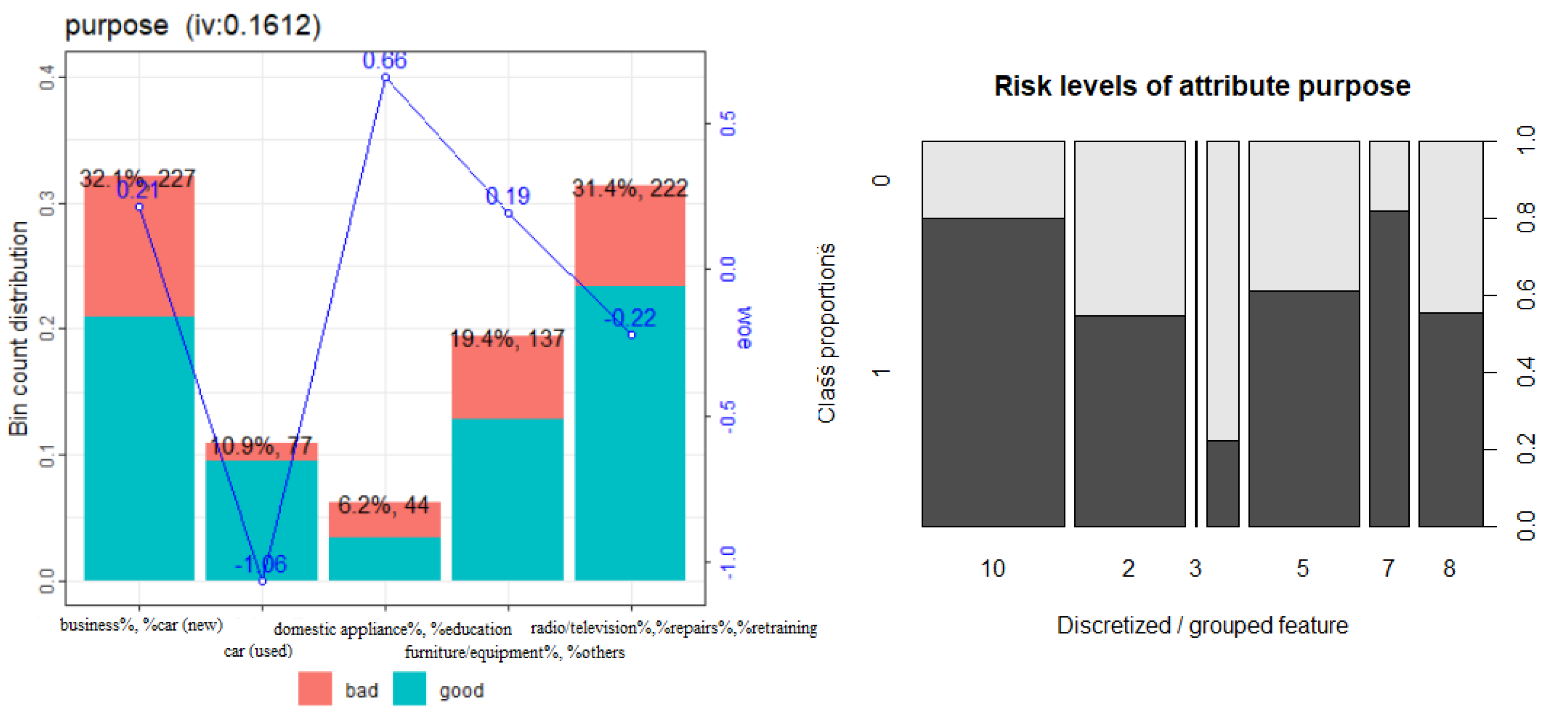
In addition to summary tables, many packages (glmdisc, riskr, Rprofet, scorecard, smbinning, woeBinning) provide a visualization of the bins on a variable level. Figure 2 (left) shows the binning resulting from code in Example 2 which is similar for most packages. A mosaic plot of the bins, which simultaneously visualizes default rates and the size of the bins, is offered by the package glmdisc (Figure 2, right) while the names of the bins after automatic binning are not self-explanatory.

3.5. Applying Bins to New Data

It has been emphasized that the bins as they are built on training data constitute the first part of a scorecard model. For this reason, it is necessary to store the results of the binning and to have functions to apply it to a data set.
Most of the packages such as scorecard (woebin_ply()), smbinning (smbinning.gen() and smbinning.factor.gen()), woeBinning (woe.binning.deploy()), creditmodel (split_bins_all()), glmdisc (discretize()) and scorecardModelUtils (num_to_cat()) provide this functionality. Example 3 illustrates the application of binning results to a data set. Via the to = “bin” argument, either bins or WoEs can be assigned:
Risks 10 00067 i003
For ctree-based binning (cf. above) a workaround using the partykit::predict.party() method for bin assignment can be obtained if the tree model is stored within the results object10.
More generally, binned variables can be created via the function cut() for numeric variables or by using lookup tables for factor variables (cf. Zumel and Mount 2014, p. 23)11. It is worth mentioning that several packages (smbinning and riskr) implement binning only on a single variable level but not simultaneously for several selected variables or all variables of a data frame12.

3.6. Binning of Categorical Variables

For categorical variables, initially, each level can be considered as a separate bin, but levels of similar default rate and/or meaning could be grouped together. As an additional challenge, there is no natural order of the levels. For these reasons, only some of the packages offer an automatic binning of categorical variables. For example, the package smbinning does not offer an automatic merging of levels for factor variables, and its function smbinning.factor() only returns the figures similar to the table resulting from Example 2. However, each original level corresponds to only one bin. The bins can be manipulated afterwards via smbinning.factor.custom() and further be applied to new data via smbinning.factor.gen(). An automatic binning of categorical variables based on conditional inference trees is supported by the packages riskr and scorecard (method = “tree”). Additional merging strategies are provided by the packages glmdisc and creditmodel (as described above), scorecard (method = “chimerge”) and woeBinning (according to similar WoEs).
Generally, merging levels with a similar default rate should only be done if the level’s frequency is large enough to result in a reliable default rate estimate on the sample. By using woeBinning’s woe.binning() function this can be ensured: Initial bins of a minimum size (min.perc.total) are created and smaller factor levels are initially bundled into a positive or negative ‘miscellaneous’ category according to the sign of the corresponding WoE which is desirable to prevent overfitting. The package scorecardModelUtils offers a separate function cat_new_class() for this. All levels less frequent than specified by the argument threshold are merged together, and a data frame with the resulting mapping table is stored in the output element $cat_class_new13. The package creditmodel provides a function merge_category which keeps the m most frequent categories and merges all other levels in a new category of name “other” but no function is available to apply the same mapping to new data.
Similar to woeBinning’s woe.binning(), the functions scorecard::woebin()14 and creditmodel::get_breaks_all()15 also merge adjacent levels of similar default rates for categorical variables. An important difference between both implementations consists in how they deal with the missing natural order of the levels and thus the notion of what ’adjacent’ means: In woe.binning() the levels are sorted according to their WoE before merging. This is not the case for the other two functions where levels are merged along their natural order which is often alphabetical 16. This might lead to an undesired binning, and as an important conclusion an analyst should think about manually changing the level order for factor variables when working with the package scorecard17.

3.7. Weights of Evidence

Most of the abovementioned packages provide WoEs of the bins within their binning summary tables. To use WoEs within the further modelling steps, it needs a functionality to assign the corresponding WoE value for each bin to the original (/or binned) variables as given by scorecard::woebin_ply() (with argument to = “woe”), woeBinning::woe.binning.deploy() (with argument add.woe.or.dum.var = “woe”) and creditmodel::woe_trans_all().
A general way of training, storing and assigning WoEs independently of the package used for binning is given by the function woe() in the klaR package, probably the first and most comprehensive implementation of WoE computation in R. WoEs for binned variables are computed on the training data and stored in an S3 object of class woe with a corresponding predict.woe() method that allows application to new data. Furthermore, via an argument ids, a subset of the variables can be selected for which WoEs are to be computed (default: all factor variables) and a real value zeroadj specified and added to the frequency of bins with empty target levels for computation of f ( ) in Equation (1) to prevent WoEs from resulting in ± . In contrast to other implementations, it allows observation weights which can be necessary for reject inference
Reject Inference to be assigned. The subsequent code shows its usage:
Risks 10 00067 i004

3.8. Short Benchmark Experiment

The example data has been used to compare the performance of the different available packages for automatic binning. For reasons explained above, binning of categorical variables requires expert knowledge on the meaning of the levels. Thus the benchmark is restricted to a comparison for the seven numeric variables in the data set. Note that four of these variables contain small numbers of distinct numeric values such as the number of credits (cf. 2nd column of Table 1). Therefore, the remaining three variables age, amount and duration are the most interesting ones. Further note that (although it is by far the most popular data set used in literature) for reasons of its size and the balance of the target levels, the German credit data might not be representative of typical credit scorecard developments (Szepannek 2017). For this reason, the results should not be overemphasized but rather used to give an idea on differences in performance of the various implementations.
Table 1 shows the number of bins resulting from automatic binning as implemented by the different packages. The first row summarizes the average number of bins for the three variables age, amount and duration. The package Rprofet (which interfaces to binr::bins.greedy(), cf. above) returns the largest numbers of bins. The number of bins as returned by the tree-based binning via smbinning and riskr as well as glmdisc and creditmodel are comparatively small.
Table 2 lists the performance of the different binning algorithms. To prevent analyzing the overfitting of the training data (as it would be obtained by increasing the number of bins), the validation data is used for comparison (cf. Example 1). To ensure a fair comparison of all packages, the performance is computed using the same methodology. First, WoEs are assigned to the binned validation data using the package klaR. Afterward, univariate Gini coefficients (as one of the most commonly used performance measures for performance evaluation of credit scoring models, cf. Section 6) of the WoE variables are computed using the package pROC (Robin et al. 2021). Note that some of the introduced functions for automatic binning allow for a certain degree ofhyperparameterization which could be used to improve the binning results. However, as the scope of automatic binning does not provide a highly tuned perfect model but rather a solid basis for a subsequent manual bin adjustment, all results in the experiment are computed using default parameterization. Further note that, for the package Rprofet, no validation performance is available as there exists no predict() method. For the packages riskr, the workaround has been used as described above to assign bins to validation data18. Concerning the results, it also has to be mentioned that the package glmdisc optimizes bins w.r.t. subsequent logistic regression based on dummy variables on the bins which further takes into account the multivariate dependencies between the variables and not just discriminative power of the single variables19.
The first column (LCL) of the results contains a 95 % lower confidence level of the best binning for each variable using bootstrapping (Robin et al. 2011). Only for the package creditmodel results of the automatic binning for the variables age, amount and duration were significantly worse (below LCL) than the best method. In summary, none of the packages clearly dominates the others, and at first glance the choice of the algorithm does not seem to be crucial. In practice, it might be worth trying different algorithms and comparing their results to support the subsequent modelling step of their manual modification (cf. above).

3.9. Summary of Available Packages for Binning

Table 3 summarizes the functionalities for variable binning and WoE assignment that are provided by the different packages as they have been worked above.
For an initial automatic binning of variables, most of the packages have implemented strategies based on decisions trees. A short benchmark experiment on the German credit data shows only small differences in performance depending on the package used. Only for the package creditmodel using default parameters was a significantly worse performance used. However, because the resulting automatically generated bins should be analyzed and modified if necesseray, the choice of an explicit algorithm for the initial automatic binning becomes less important. In summary, the package woeBinning offers quite a comprehensive toolbox with many desirable implemented functionalities, but unfortunately no manual modification of the results from automatic binning is supported. For the latter the scorecard package can be used, but it must be used with care for factor variables because its automatic binning of categorical variables suffers from dependence on the natural order of the factor levels. As a remedy, a function has been suggested in the supplementary code (cf. footnote 17) to import the results of woeBinning’s automatic binning into the result objects from the scorecard package for further processing.

4. Preselection of Variables

4.1. Overview

As outlined above, a major aspect of credit risk scorecard development is to allow for the integration of expert domain knowledge at different stages of the modelling process. In statistics, traditionally criteria such as AIC or BIC are used for variable selection to find a compromise between a model’s ability to fit the training data’s parsimony in terms of the number of trainable model parameters (cf. Section 5). For scorecard modelling, typically a variable preselection is made, which allows for a plausibility check by analysts and experts. Apart from plausibility checks, several analyses are carried out at this stage, typically consisting of:
  • Information values of single variables;
  • Population stability analyses of single variables on recent out-of-time data
  • Correlation analyses between variables.

4.2. Information Value

Variables with small discriminatory power in terms of their IV (cf. Section 3) are candidates for removal from the development process. While the interpretation “small” in the context of IV slightly varies depending on who is asked, an example is given in Siddiqi (2006) by I V < 0.02 . As an important remark and in contrast to a common practice in credit scorecard modelling, in business not just the IV of a variable should be taken into account but rather how much different information a variable will contribute to a scorecard model that is not already included in other variables. For this reason, IVs should be analyzed together with correlations (cf. this Section below). If not just validation data but also an independent test data set is available, a comparison of the IV on training and validation data can be used to check for overfitting of the binning.
Table 4 lists packages that provide functions to compute information values of binned variables. As usual, these packages differ by the type of the target variable that is required. Some allow for factors; others require binary numerics that take the values 0 and 1. An important difference consists in whether (and how) they do WoE adjustment in case of bins where one of the classes is empty. In creditR no adjustment is completed, and the resulting IV becomes . Some packages (creditmodel, Information, InformationValue and smbinning) return a value different from , but from the documentation it is not clear how it is computed. For the packages scorecard and scorecardModelUtils, the adjustment is known, and for the package klaR the adjustment can be specified in an argument. Note that, depending on the adjustment, the resulting IVs of the affected variables may differ strongly.
Example 5 shows how IVs can be computed using the package klaR with zero adjustment (which in fact is not necessary here.) The function woe() (cf. Example 4) automatically returns IVs for all factor variables.
Risks 10 00067 i005
The package creditR also offers a function IV_elimination() that allows an iv_threshold and returns a data set with a subset of variables with IV above threshold for the training data. Similarly, the package scorecardModelUtils offers a function iv_filter() that returns a list of variable names that pass (/fail) a prespecified threshold.
Beyond computation of IVs, the package creditR can be used to compute Gini coefficients for simple logistic regression models on each single variable via the function Gini.univariate.data(), and just as for IVs, this can be used for variable subset preselection (Gini_elimination()). The function pred_ranking() from the package riskr returns a summary table containing IV as well as the values of the univariate AUC and KS statistic and an interpretation.

4.3. Population Stability Analysis

To take into account the sample selection bias that results from a customer portfolio shift (e.g., due to new products or marketing activities), the stability of the distribution of the variable’s bins over time is considered. For this purpose, typically, the population stability index (PSI) is computed between the (historical) development sample data and a more recent out-of-time (OOT) sample (where typically performance information is not yet available). Basically, the PSI is just the IV (cf. eqn. (2)). While the IV compares two data sets given by the development sample which are split according to the levels of the target variable ( y = 1 vs.  y = 0 ), the PSI compares the entire development sample ( y { 0 , 1 } ) with an entire out-of-time sample. A large PSI indicates a change in the population w.r.t. the bins. A small PSI close to 0 indicates a stable population and (again referring to Siddiqi (2006)) P S I < 0.1 can be interpreted as stable while a P S I > 0.25 is an indicator of a population shift. Of course, a decision of inclusion or removal of variables from the development sample should take into account both population stability and the discriminatory power (i.e., IV) of a variable. With reference to the analogy for PSI and IV, the formerly presented functions of IV calculation can also be used for population stability analysis. The function SSI.calc.data() from the package creditR returns a data frame of PSIs for all variables. The corresponding code (here, for a computation of PSIs between training and validation—not OOT—set) is given in Example 6.
Risks 10 00067 i006
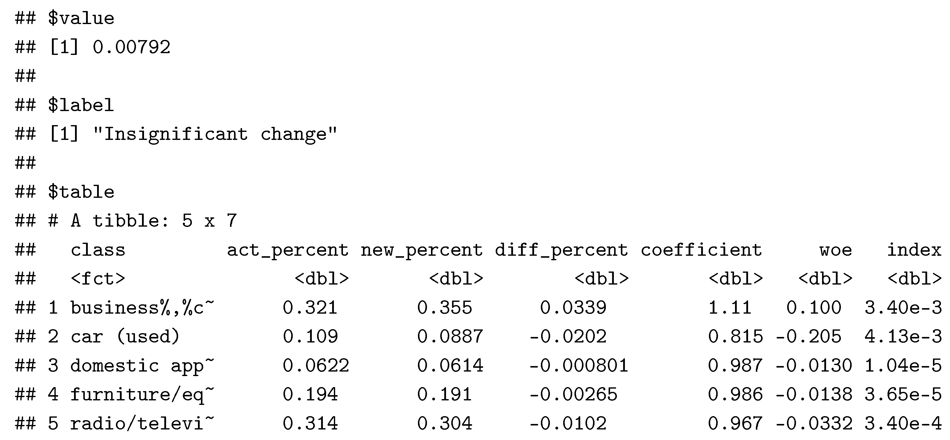
The function riskr::psi() calculates the PSI for single variables and also provides a more detailed table on the bin-specific differences (cf. Example 7 for the variable purpose). It does contain the absolute and relative distribution of the bins (for reasons of space two columns with the absolute frequencies have been discarded from the output). The PSI of the variable as given by the value element of the output corresponds to the sum of the column index:
Risks 10 00067 i007
Risks 10 00067 i008
Alternatively, the package smbinning comes along with a function smbinning.psi(df, y, x) which requires both development and OOT sample to be in one data set (df) and a variable y that indicates the data set where an observations originates. In addition to a function get_psi_all() for PSI calculation, the package creditmodel provides a function get_psi_plots() to visualize stability of the bins for two data sets using bar plots with juxtaposed bars. The packages creditR and scorecard further offer functions that can be used for an OOT stability analysis of the final score (cf. Section 5).

4.4. Correlation Analysis

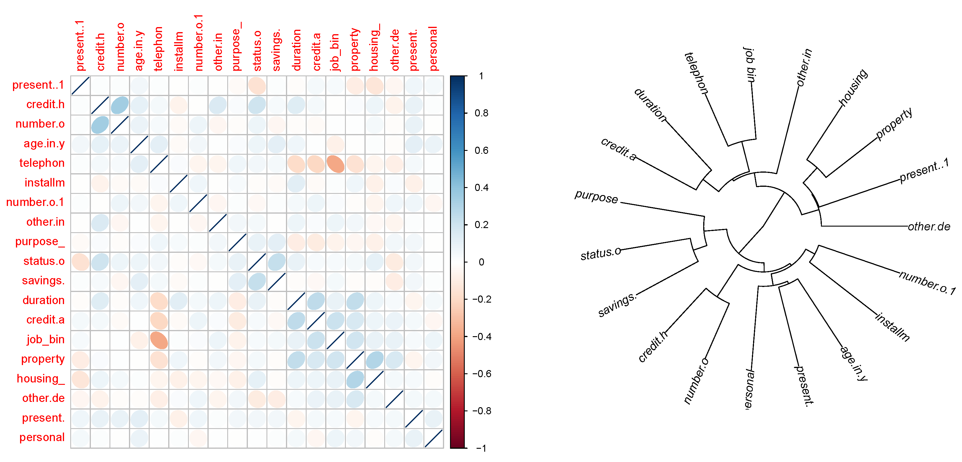
To avoid variability of the estimates of a regression model, its regressors should be of low correlation (cf. e.g., Hastie et al. 2009, chps. 3, 4). As per construction, WoE transformed variables are linear in the logit of the target variable, providing a natural approach in analyzing correlations between these variables. For this purpose, the caret package (Kuhn 2008, 2021) offers a function findCorrelation() that automatically identifies among any two variables of strong correlation the one that has the larger average (absolute) correlation to all other variables. A major advantage of performing correlation analysis in advance for variable preselection is that it can be used as another way to integrate expert’s experience into the modelling. Among variable clusters of high correlations, experts can choose which of these variables should be used or discarded for further modelling. There are some packages that are not originally intended to be used for credit scorecard modelling but that offer functions that can be used for this purpose. The package corrplot corrplot offers a function to visualize the correlation matrix and resort it such that groups of correlated variables are next to each other (cf. Figure 3, left). An alternative visualization is given by a phylogenetic tree of the clustered variables using the package ape (Paradis and Schliep 2018; Paradis et al. 2021), where the variable clustering is obtained using the package ClustOfVar ((Chavent et al. 2012, 2017), cf. Figure 3, right). The code for creation of both plots is given in the following example (note that the choice of the hclust.method = “complete” in the left plot guarantees a minimum correlation among all variables in a cluster, but all correlations on the training data are below 0.35 in this example).
Risks 10 00067 i009
Risks 10 00067 i010
The package clustVarLV (Vigneau et al. 2015, 2020) offers variable clustering such that the correlation between each variable and the first latent principal component of its variable cluster is maximized. The number of clusters K has to be prespecified. As it can be seen in the output from Example 9 (only cluster 1 is shown), for each variable the correlation to the cluster’s latent component as well as the correlation to the ‘closest’ next cluster are shown.
Risks 10 00067 i011
Risks 10 00067 i012
Among the aforementioned packages dedicated to credit scoring, creditR contains a function variable.clustering() that performs cluster’s pam (Maechler et al. 2021) on the transposed data for variable clustering. The (sparsely documented) function correlation.cluster() %data, output, “variable”, “Group”)} can be used to compute average correlations between the variables of each cluster. 20
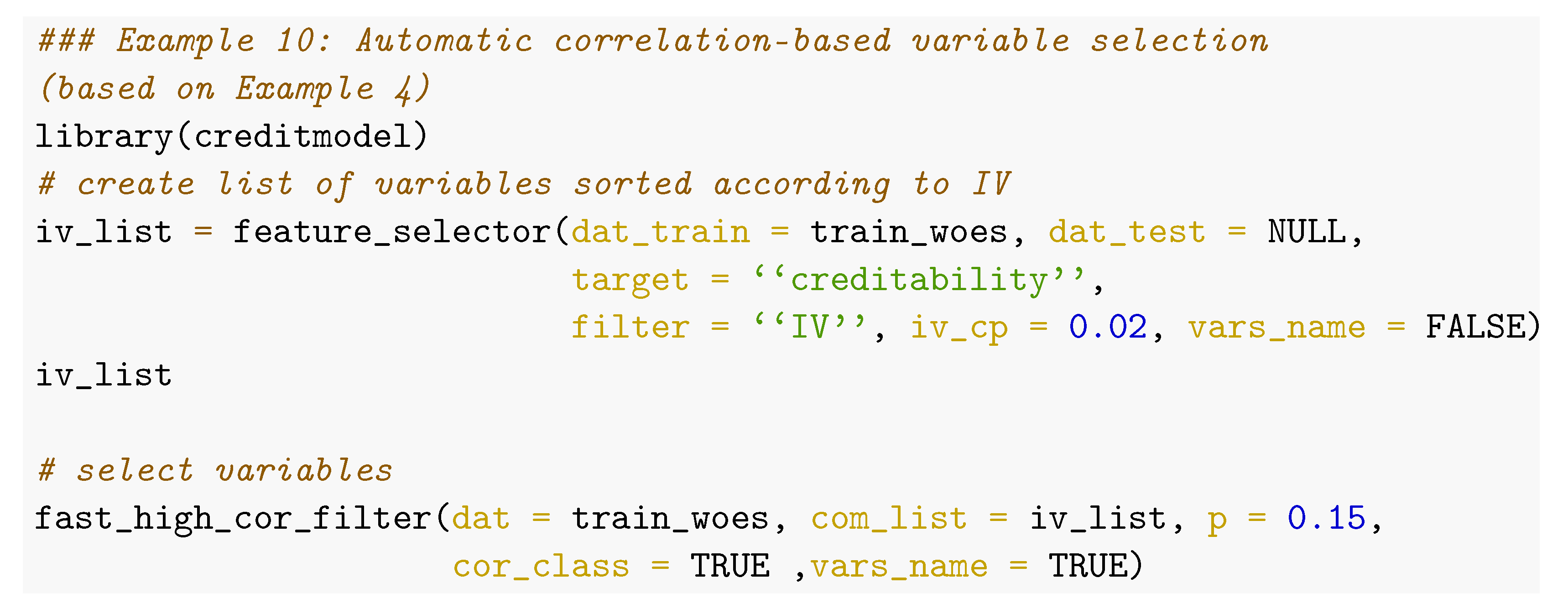
The package Rprofet provides two functions WOEClust_hclust() and WOEClust_kmeans() that perform stats::hclust() on the transformed data or ClustOfVar::kmeansvar() and return a data frame with variable names and cluster index together with the IV of the variable, which may help to select variables from the clusters. Unfortunately, they are only designed to work with output from the package’s function WOEProfet() and require a list of a specific structure as input argument. In addition to functions cor_plot() for visualization of the correlation matrix, char_cor() computes a matrix of Cramer’s V between or a set of categorical variables and get_correlation_group() for detection of groups of correlated (numeric) variables. The package creditmodel also contains a function fast_high_cor_filter() for an automatic correlation- based variable selection. In a group of highly correlated variables, the one with the highest IV is selected as shown in Example 10.
Risks 10 00067 i013
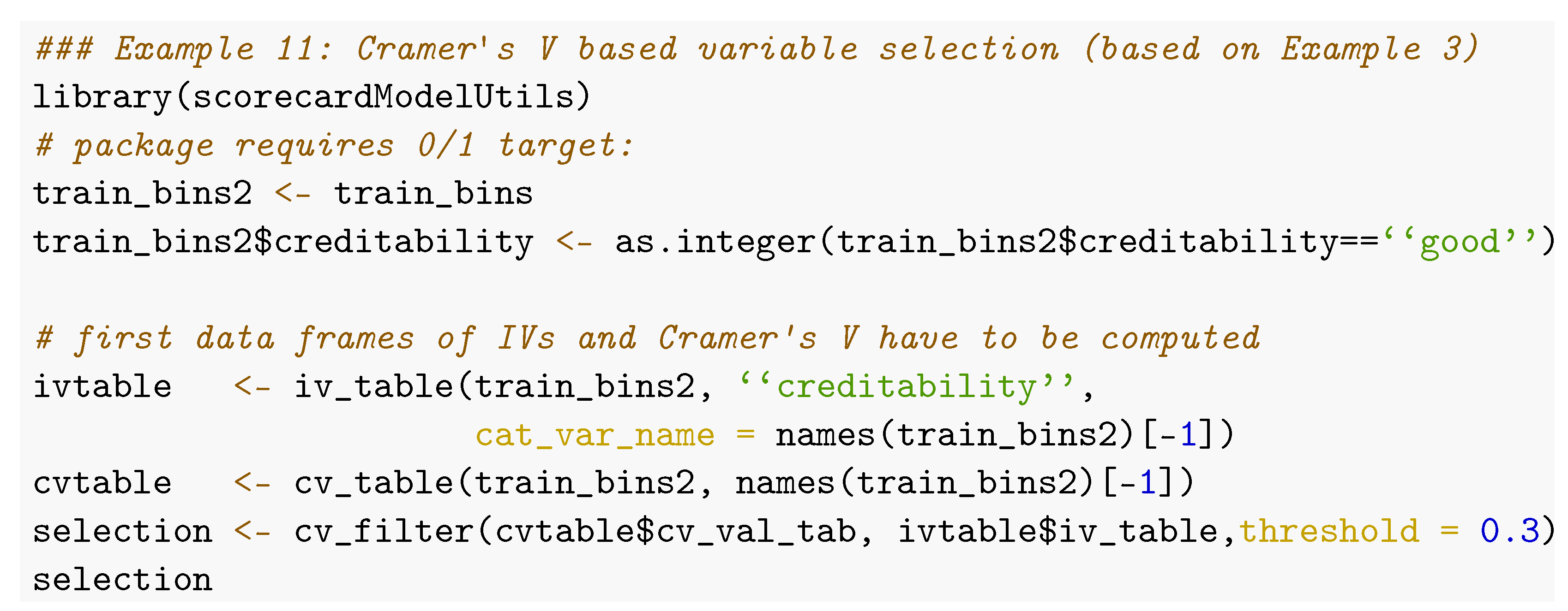
Similarly, the package scorecardModelUtils offers an alternative for an automatic variable preselection based on Cramer’s V using the function cv_filter(). Among two (categorical) variables of V >  threshold, the one with lower IV is automatically removed (cf. Example 11). Finally, two functions, iv_filter() and vif_filter() can be used for variable preselection based on IVs only (w/o taking into account for correlations between the explanatory variables) and based on variance inflation (cf. also Section 5).
Risks 10 00067 i014

4.5. Further Useful Functions to Support Variable Preselection

The package scorecard contains a function var_filter() that performs an automatic variable selection based on IV and further allows for specifying a maximum percentage of missing or identical values within a variable, but it does not account for correlations among the predictor variables. Alternatively, the package creditmodel has a function feature_selector() for automatic variable preselection based on IV, PSI, correlation and xgboost variable importance (Chen and Guestrin 2016).
The package creditR has two functions to identify variables with missing values (na_checker()) and compute the percentage of variables with missing values (missing_ratio()). For imputation of numeric variables in a data set with mean or median values, a function na_filler_contvar() is available. Of course, this has to be handled with care as the mean or median value will typically not be the same on training and validation data. The package mlr (Bischl et al. 2016, 2020) offers imputation that can be applied to new data.
For an assignment of explicit values to missing the package scorecardModelUtils also provides a function missing_val(). This can be either a function such as “mean”, “median” or “mode” or an explicit value such as -99999 which can be meaningful before binning to assign missing values to a separate bin. Similarly, for categorical variables the assignment of a specific level such as “missing_value” can be meaningful. A function missing_elimination() removes all variables with a percentage above missing_ratio_threshold from training (but not from validation) data. The package creditmodel offers a convenient function data_cleansing() that can be used for automatic deletion of variables with low variance and a high percentage of missing values, to remove duplicated observations and reduce the number of levels of categorical variables. The package riskr provides two functions select_categorical() and select_numeric() to select all (non-/) numeric variables of a data frame.
A univariate summary of all variables is given by the function univariate() of the scorecardModelUtils package. A summary for numeric variables can be computed using the function ez_summ_num() from the package riskr. A general overview of packages explicitly designed for exploratory data analysis that provide further functionalities are given in Staniak and Biecek (2019). The packages scorecard (one_hot() and var_scale()) and creditmodel (\texttt{one_hot_encoding(), de_one_hot_encoding(), min_max_norm()) provide functions for one-hot-encoding of categorical and standardization of numeric variables.

5. Multivariate Modelling

5.1. Variable Selection

Traditionally, credit risk scorecards are modelled using logistic regression (cf. e.g., Anderson 2019; Siddiqi 2006; Thomas et al. 2019; Wrzosek et al. 2020), which is in R performed via glm() (with family = binomial). In addition to the manual variable preselection as described in the former section, typically, a subsequent variable selection is performed which can be completed by the step() function. Common criteria for variable selection are AIC (k = 2) or BIC (k = log(nrow(data))). Example 12 gives an example for BIC based variable selection.
Risks 10 00067 i015
Note that an initial model (here: null) and the scope for the search have to be specified. This offers another possibility for expert knowledge integration. After each step the criteria of all candidates are reported and can be used to decide among several variable candidates of similar performance for the one that is most appropriate from a business point of view. The corresponding variable can be manually added to the formula of a new initial model in a subsequent variable selection step.
The function smbinning.logitrank() of package smbinning runs all possible combinations of a specified set of variables, ranks them according to AIC and returns the corresponding model formulas in the result data frame. Depending on the size of the preselected set of variables (cf. Section 4), this can be time-consuming.
As an alternative to AIC and BIC, Scallan (2011) presents how variables can be selected in line with the concept of information values (cf. Section 3) using so-called marginal information values, but currently none of the presented packages offers an implementation of this strategy.
It is also common to consider the variance inflation factor of the explanatory variables of a final model given by:
V I F ( X i ) = 1 1 R i 2
where R i 2 is the R 2 of a linear regression model with X i as dependent variable and all other explanatory variables except X i as regressors. Large values of V I F ( X i ) denote that this variable can be explained by the other regessors and are an indication of multicollinearity. Both the packages car (Fox and Weisberg 2019; Fox et al. 2021) and scorecard offer a function vif() that can be used for this purpose as well as the functions vif.calc() and lr_vif() of the packages creditR and creditmodel (cf. Example 13).
Risks 10 00067 i016
Not only variable selection during the scorecard development but also the question of segmentation may arise, i.e., whether one single model or several separate models should be used for different subsets of the population. For this purpose, the package glmtree offers a function glmtree() that computes a potential segmentation scheme according to a tree of recursive binary splits where each leaf of the tree consists in a logistic regression model. The resulting segmentation optimizes AIC, BIC or alternatively the likelihood or the Gini coefficient on validation data. Note that this optimization does not account for variable selection as described above.

5.2. Turning Logistic Regression Models into Scorecard Points

From the coefficients of the logistic regression model, the historical shape of a scorecard is obtained by assigning the corresponding effect (aka points) to each bin (such that the score of a customer is the sum over all applicable bins and can easily be calculated by hand). Typically, the effects are scaled to obtain some predefined points to double the odds (pdo, cf. e.g., Siddiqi 2006) and rounded to integers.
The package scorecard offers a function scorecard() that translates a glm object into scorecard points as described above and in addition returns key figures such as frequencies, default rates and WoE for all bins. A function scorecard_ply() is available that can be used to assign scores to new data. In addition to the glm object, the bins as created by scorecard’s woebin() (cf. Section 3) have to be passed as an input argument. Further arguments do specify the (pdo) as well as a fixed number of points points0 that corresponds to odds of odds0 and whether the scorecard should contain an intercept or whether the intercept should be redistributed to all variables (basepoints_eq0). The function requires WoEs (not just the binned factors) and the variable names in the coef(glm) to match the convention of variable renaming as it is done by scorecard’s woebin_ply() function (i.e., a postfix _woe)21.
Alternatively, a function scorecard2() is available that directly computes a scorecard based on bins and a data frame of the original variables. Here, in addition, the name of the target variable (y) and a named vector (x) of the desired input variables have to be passed22. Example 14 illustrates the usage of scorecard2() and its application to new data (here represented by the validation set) as well as its output for the variable duration.in.month.
Risks 10 00067 i017
Risks 10 00067 i018
Risks 10 00067 i019
In addition, the package further contains a function report() that takes the data, the (original) names of all variables in the final scorecard model and a breaks list (cf. Section 3 that can be obtained from the bins) as input arguments and generates an excel report summary of the scorecard model. Different sheets are reported with information and figures on the data, model, scorecard points, model performance and the binning figures for all variables of the model which can be used for model development documentation in practice.
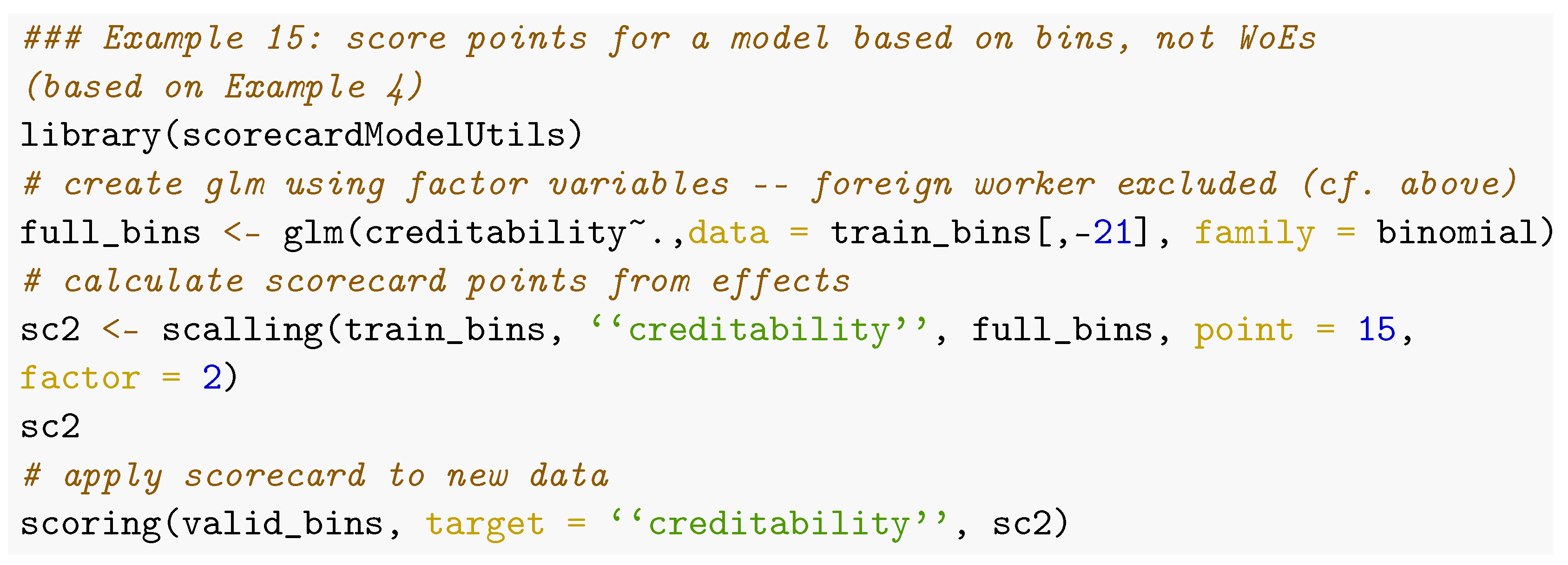
To translate a glm based on factor variables (bins instead of WoEs) into scorecard points, the package scorecardModelUtils provides a function scalling(). Its output can be used to predict scores for new data by function scoring() (cf. Example 15).
Risks 10 00067 i020
The package creditmodel transforms a glm object into scorecard points via a function get_score_card(), which requires a bin table created by creditmodel::get_bins_table_all() and thus is restricted to application within its own universe. In addition, if a table of scorecard points is not required, it offers a function score_transfer() that directly applies the glm object to data and scales the resulting points accordingly (cf. Example 16) and another function p_to_score to turn posterior probabilities into score points.
Risks 10 00067 i021
Another implementation of calculating scorecard points from a glm object based on bins and not WoEs is given by the function smbinning.scaling(), which comes with a predict function smbinning.scoring.gen() that can be used to score new observations but that requires the binned variables have been generated with smbinning.gen() or smbinning.factor.gen() (cf. Section 3). A function smbinning.scoring.sql() is available that transforms the resulting scorecard into SQL code.
The package Rprofet also contains a function ScorecardProfet() for this purpose, which calculates a glm with corresponding scorecard points but only based on binning and WoEs as calculated by functions from the package itself (cf. Section 3), and no function is available for application of the scorecard points to new data. The function scaled.score() of the package creditR transforms posterior default probabilities into scores where any increase points double the odds (of nondefault), and odds of increase correspond to ceiling_score points. In addition, the package creditR offers a function that can be used to recalibrate an existing glm on calibration data. A simple logistic regression is fit on the calibration_data with only one input variable: the predicted log odds by the current model.

5.3. Class Imbalance

In credit scorecard modelling, the class typically is highly unbalanced in the training sample. This issue has been addressed in several papers (Brown and Mues 2012; Crone and Finlay 2012; Vincotti and Hand 2002). Usual remedies are oversampling, undersampling, synthetic minority over-sampling (SMOTE, Chawla et al. 2002) or simply reweighing observations. A comprehensive benchmark study of these techniques as well as overbagging is undertaken in Bischl et al. (2016), and it turns out that logistic regression is less sensitive to class imbalance than tree-based classifiers. Furthermore, note that different from, e.g., the accuracy of the two most commonly used performance measures in credit scorecard modelling, the Gini coefficient and the KS statistic (cf. Section 6) do not depend on the class imbalance ratio.
The package klaR allows for specifying observation weights for WoE computation (see Section 3.7). Within the mlr3 framework, imbalance correction can be performed using mlr3pipelines (Binder et al. 2021). Several resampling algorithms are implemented in the packages imbalance (Cordón et al. 2020, 2018) and unbalanced (Pozzolo et al. 2015). The SMOTE algorithm is also implemented in the smotefamily package (Siriseriwan 2019).

6. Performance Evaluation

6.1. Overview

In credit scoring modelling, performance evaluation is used not only for model selection but also for third-party assessments of an existing model by auditors or regulators and to drive future management decisions about whether an existing model should be kept in place or whether it should be replaced by a new one. Note that, as opposed to common practice in machine learning, hyperparameter tuning typically has no separate validation data used for model selection (cf. e.g., Bischl et al. (2012), Bischl et al. (2021)), but in credit scorecard modelling, the validation data serves for independent model validation (corresponding to test data in frameworks such as mlr3). While this is less critical in the case of simple models such as logistic regression, it should still be kept in mind, especially if the model is benchmarked against more flexible machine learning models such as support vector machines, random forests or gradient boosting (cf. e.g., Hastie et al. (2009)).

6.2. Discrimination

The two most popular performance metrics for credit scorecards are the Gini coefficient, G i n i = 2 ( A U C 0.5 ) and the Kolmogorov–Smirnov test statistic. While for the latter, R provides the function ks.test(), one of the most popular ways to compute the AUC in R is given by the package ROCR (Sing et al. 2005, 2020). Nonetheless, for the purpose of credit scorecard modelling, it is referred to the package pROC at this point for the following three reasons:
  • Different from standard binary classification problems, credit scores are typically supposed to be increasing if the event (= default-) probability decreases. The function roc() of the package pROC has an argument direction that allows for specifying this.
  • In credit scoring applications, it may be given that not all observations of a data set are of equal importance, e.g., it may not be as important to distinguish which of two customers with small default probabilities has the higher score if his or her application will be accepted anyway. The package’s function auc() has an additional argument partial.auc to compute partial area under the curve (Robin et al. 2011).
  • Finally, its function ci() can be used to compute confidence intervals for the AUC using either bootstrap or the method of DeLong (DeLong et al. 1988; Sun and Xu 2014), e.g., to support the comparison of two models.
Example 17 demonstrates how pROC can be used for performance analysis.
Risks 10 00067 i022
Risks 10 00067 i023
Risks 10 00067 i024
Among the packages enumerated above, creditR offers a function Kolmogorov–Smirnov(), and riskr has two functions, ks() and ks2(), for computation of the Kolmogorov–Smirnov test statistic. In addition, riskr provides a function divergence() to compute the divergence between two empirical distributions as well as gg_dists() and gg_cum() to visualize the score densities for defaults and nondefaults and their empirical cumulative distribution functions. To compute the Gini coefficient, the package riskr provides functions aucroc (AUC), gini (Gini coefficient), gg_roc() (visualization of the ROC curve), gain() (gains table for specified values on the x-axis) and gg_gain() /gg_lift() (for visualization of the gains-/lift-chart).
In the package creditmodel, two functions ks_value() and auc_value() are available as well as a model_result_plot() to visualize the ROC curve, cumulative score distributions of defaults vs. nondefaults, lift chart and the default rate over equal-sized score bins. A table with respective underlying numbers can be obtained via perf_table().
The package InformationValue contains two functions, ks_stat() and ks_plot(), for Kolmogorov-Smirnov analysis and several functions: AUROC(), plot_ROC(), Concordance() and SomersD() (Gini coefficient) to support analyses with regard to the Gini coefficient. Additionally, the confusionMatrix() and derivative performance measures misClassError(), sensitivity(), specificity(), precision(), npv(), kappaCohen() and youdensIndex() (cf. e.g., Zumel and Mount (2014) chp. 5 for an overview) can be computed for a given cut off by the corresponding functions. Note that these measures are computed with respect to the nondefault target level (supposed to be coded as ‘1’ in the target variable) as well as a cut off optimization w.r.t. the misclassification error, Youden’s Index or the minimum (/maximum) score such that no misclassified defaults (/non-defaults) occur in the data (function optimalCutoff()).
Similar measures (accuracy, precision, recall, sensitivity, specificity, F1) are computed by the function fn_conf_mat() of the scorecardModelUtils package. Numeric differences between the (0/1-coded) target and the model’s predictions in terms of MSE, MAE and RMSE can be computed by its fn_error() function. The package boottol contains a function boottol() to compute bootstrap confidence intervals for Gini, AUC and KS, where subsets of the data above different cut off values are also considered. It may be desirable to analyze the (cumulative) frequencies of the binned scores. A table of such frequencies is returned by the function gini_table() in the scorecardModelUtils package. Example 18 shows selected columns for a binned score using the function gains_table() from the scorecard package.
Risks 10 00067 i025
Risks 10 00067 i026
Risks 10 00067 i027
Note that although the Gini coefficient is generally bounded by −1 and 1, the value it can take for a specific model strongly depends on the discriminability of the data. For this reason, it is suitable to compare performance on different models on the same data rather than comparing performance across different data sets. Consequently, for the purpose of an out-of-time monitoring of a scorecard, it is advisable to compare an existing scorecard’s performance against a recalibrated version of it rather than to compare it with its performance on the original (development) data. Drawbacks of the Gini coefficient as a performance measure for binary classification are discussed in (Hand 2009), and the H-measure is proposed as an alternative which is implemented in the package hmeasure (Anagnostopoulos and Hand 2019). The expected maximum profit measure (Verbraken et al. 2014) as implemented in the package EMP (Bravo et al. 2019) further takes into account the profitability of a model.

6.3. Performance Summary

Many of the functionalities as provided by the packages for scorecard modelling in the previous subsection already exist in other packages and are thus not indispensable. In addition to these, however, some of the package provide performance summary reports of several performance measures. These functions are listed in the following table.
In Example 19, computation of a scorecard performance summary is demonstrated using the package smbinning (which returns the largest number of performance measures of the four functions from Table 5) as well the function riskr::gg_perf() that can be used to produce several graphs on the scorecard’s performance (cf. Figure 4). Note that although ROC curves are one of the most popular tools for performance visualization of binary classifiers, they are hardly suited to visualize the performance difference of several competitive models. One reason for this is that large areas of the TPR-FPR plane (e.g., everything below the main diagonal) are typically of no interest given a specific data situation. For this reason, in practice, ROC curves are not very useful for model selection.
Risks 10 00067 i028

6.4. Rating Calibration and Concentration
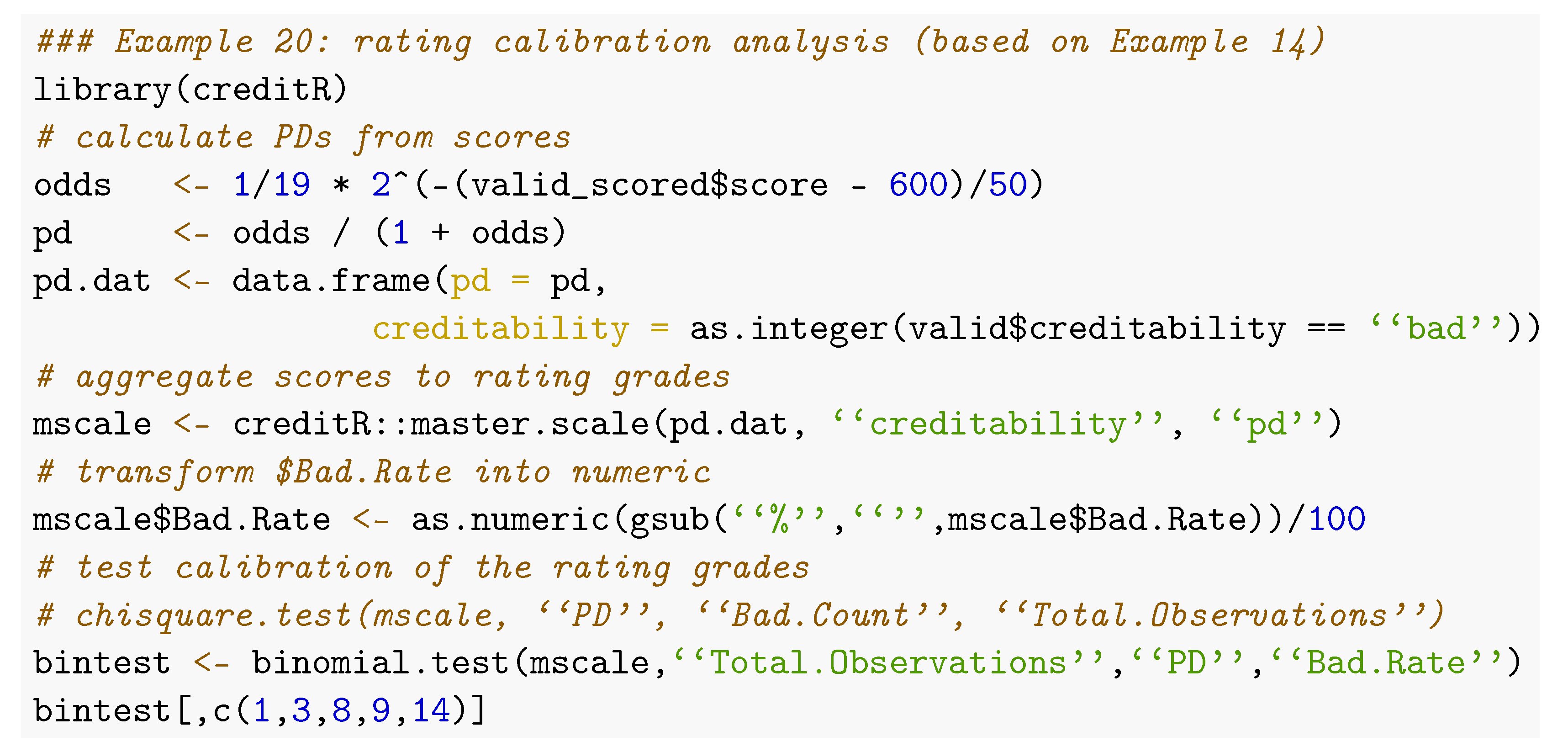
From a practical point of view, it is often desirable to aggregate scorecard points into classes (rating grades) of similar risk, which is once again a binning task (cf. Section 3). The package creditR contains a function master.scale() that takes a data frame with scores and corresponding default probabilities as input and uses the function woeBinning::woe.binning() to group scores of similar WoE (cf. Example 20). The function odds_table() of the riskr package allows setting a breaks argument with arbitrary bins.
Rating classes should be appropriately calibrated in the sense that the predicted and observed default probabilities match for all rating grades. In order to check this, the package creditR contains three functions (chisquare.test(), binomial.test() and adjusted.binomial.test()) that provide a table with indicators for each rating grade (cf. Example 19). Another function, binomial.point(), compares the observed average predicted default probability on the data with prespecified boundaries around some desired central tendency default probability. Bootstrap confidence intervals for default probabilities of rating grades can be computed using the function vas.test() of the package boottol. A Hosmer–Lemeshow goodness-of-fit test (Hosmer and Lemeshow 2000) is, e.g., implemented by the function hoslem.test() in the resourceselection package (Lele et al. 2019).
Risks 10 00067 i029
Risks 10 00067 i030
According to regulation, ratings must avoid risk concentration (i.e., a majority of the observations being assigned to only a few grades). The Herfindahl–Hirschman index ( H H I = j f ^ ( j ) 2 , with the empirical distribution f ^ of the rating grades j) can be considered to verify this, as e.g., implemented by creditR’s Herfindahl.Hirschman.Index() or Adjusted.Herfindahl.Hirschman.Index(). Small values of HHI indicate low risk concentration.

6.5. Cross Validation

Some of the mentioned packages also provide functions for cross-validation. As both binning and variable selection are interactive, they are not suited for cross-validation (cf. Section 3 and Section 4). For this reason it should be used on the training data and restricted to analyzing overfitting of the logistic regression model. There are already several packages available that provide general functionalities for execution of cross-validation analyses (e.g., mlr3 or caret). The function k.fold.cross.validation.glm() of the creditR package computes cross-validated Gini coefficients, while the function perf_cv() of the scorecard package offers an argument to specify different performance measures such as “auc”, “gini” and “ks”. Both functions allow setting seeds to guarantee reproducibility of the results. The function fn_cross_index() somewhat more generally returns a list of training observation indices that can be used to implement a cross-validation and compare models using identical folds.

7. Reject Inference

7.1. Overview

Typically, the final stage of scorecard development consists of reject inference. The scorecard model is based on historical data but already in the past, credit applications of customers that were assumed to be high risk were rejected, and thus for these data only, the predictor variables are available from the application but not the target variable. The use of these observations with unknown performance is commonly referred to as reject inference.
The benefits of using reject inference in practice still remains questionable. It has been investigated by several authors (cf. e.g., Crook and Banasik (2004), Banasik and Crook (2007), Verstraeten and den Poel (2005), Bücker et al. (2013), Ehrhardt et al. (2019)) and is nicely discussed in Hand and Henley (1993). The appropriateness of different suggested algorithms for reject inference depends on the way the probability of being rejected can be modelled, i.e., whether it is solely a function of the scorecard variables (MAR) or not (MNAR) (for further details cf. also Little and Rubin (2002)). A major issue is that, especially for the most relevant MNAR situation, the inference entirely relies on expert judgments. For this reason the appropriateness of the model cannot be tested anymore. In consequence, reject inference should be used with care.
In R, the only package that offers functions for reject inference is the package scoringTools, which is available on Github but not on CRAN. It provides five functions for reject inference: augmentation(), fuzzy_augmentation(), parcelling(), reclassification() and twins(), which correspond to common reject inference strategies of the same name (cf. e.g., Finlay (2012)). In the following, two of the most popular strategies, namely augmentation and parcelling are briefly explained as they are implemented within the package, completed by an example of their usage.

7.2. Augmentation

An initial logistic regression model is trained on the observed data of approved credits (using all variables, i.e., variable selection has to be done in a preceding step). Afterward, weights are assigned to all observations of this sample of accepted credits, according to their probability of being approved. For this purpose, all observations (accepted and rejected) are scored by the initial model. Then, score-bands are defined and within each band23 the probability of having been approved is computed by the proportion of observations with known performance in the combined sample from both accepted and rejected credits. Finally, the logistic regression model is fitted again on the sample of the accepted loans with only observed performance but reweighted observations24.

7.3. Parcelling

Based on an initial logistic regression model which is trained on the observed data of approved credits, only score-bands are defined, and the observed default rate P D ^ j of each score-band j is derived. The observations of the rejected subsample are then scored by the initial model and assigned to each score-band. Labels are randomly assigned to the rejected observations such that they will have a default probability of P D ^ j × α j 25 in each band where α j are user-defined factors to increase the score-bands’ default rates which have to be specified by expert experience. Typically the α j are set to be increasing for score-bands with larger default probabilities. Note that accepting these credit applications in the past might have happened for reasons beyond those that were reflected by the score variables but which led to a reduced risk for these observations in the observed sample compared to observations with a similar score in the total population. For this reason, parcelling is suitable for the MNAR situation.
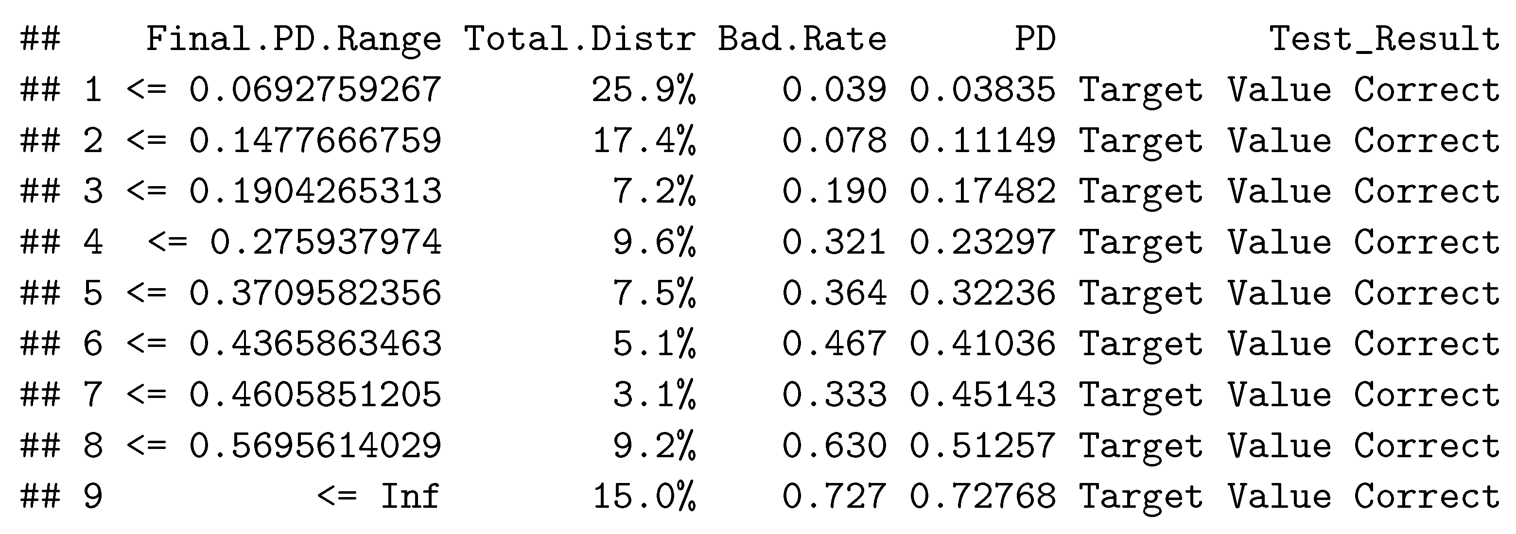
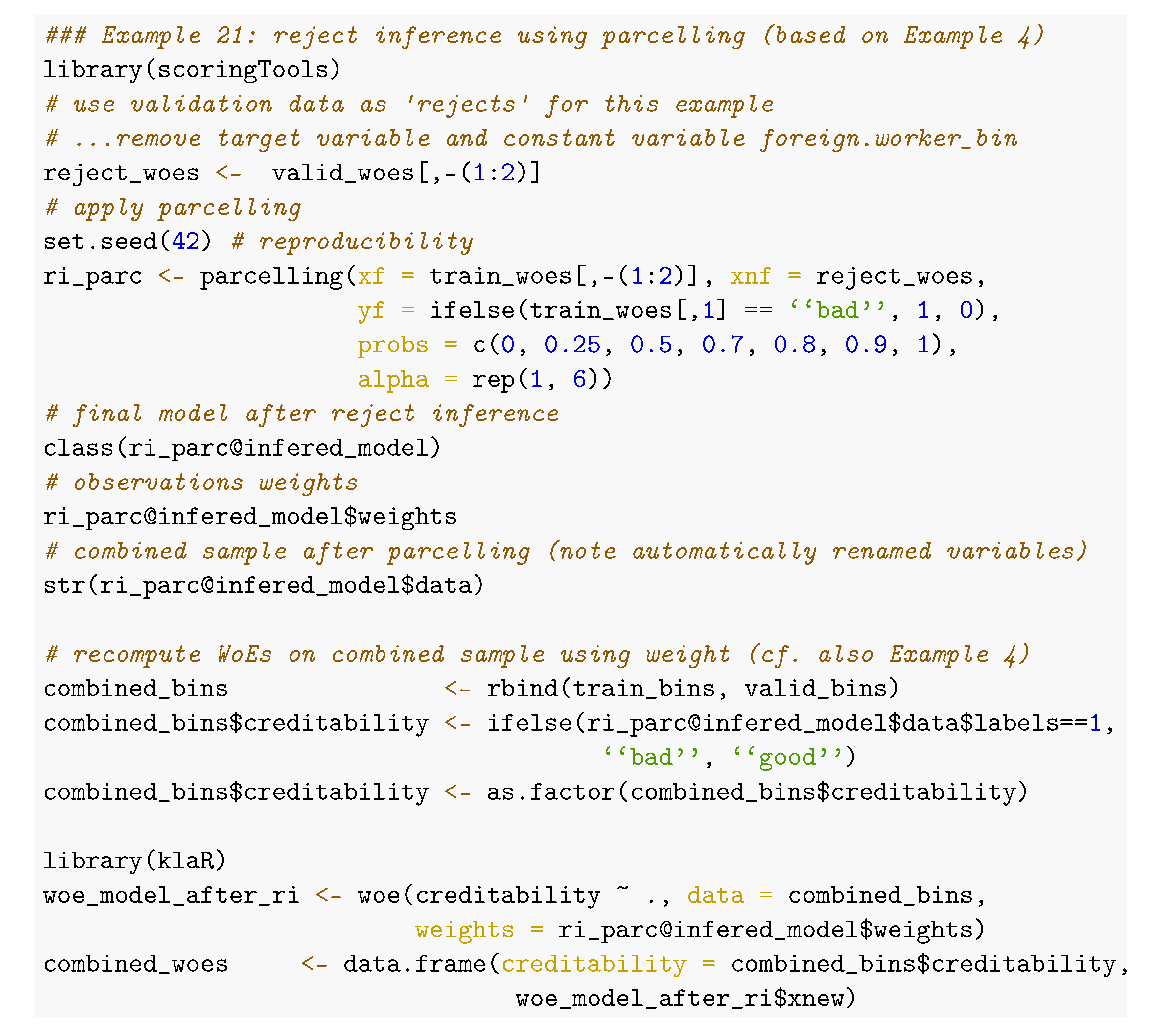
Example 21 illustrates parcelling using the scoringTools package. Note that all other functions of this package are of similar syntax and output. For parcelling in particular, the probs argument specifies quantiles w.r.t. the predicted default probabilities (i.e., from low risk to high risk). Although in the example the factor vector alpha is constantly set to 1 for all bands, in practice it will be chosen to be increasing, at least for quantiles of high PDs.
Risks 10 00067 i031
The initial model and the final model are stored in the result object’s slots financed_model and infered_model. Both are of class glm. Note that both models are automatically calculated without any further options of parameterization such as variable selection or a recomputation of the WoEs based on the combined sample of accepted applications and rejected applications with inferred target. For this purpose, the woe() function of the klaR package can be used, which supports the specification of observation weights as the only one among all presented packages. Finally, the combined sample can be used to rebuild the scorecard model as described in Section 4, Section 5 and Section 6.

8. Summary and Discussion

For a long time in the R universe, no packages were available that were explicitly dedicated to the credit risk scorecard development process, while during the last few years a simultaneous growth of several packages on this task has been observed. Some of these packages are available on CRAN, while some are only available on Github.
This paper aims to give a comparative overview on the different functionalities of currently available packages guided by the sequence of steps along a typical scorecard development process. At the same time, any required functionality is available, which makes it easy to develop scorecards using R. As a conclusion of this systematic review, currently the most comprehensive implementations are given by the packages scorecard, scorcardModelUtils, smbinning and creditmodel. With regard to the important modelling step of variable binning and WoE computation, the package woeBinning provides an implementation that reflects a broad range of practical issues (cf. Section 3). The package creditmodel comes with a whole set of additional functionalities such as cohort analysis, correlation based variable preselection or Cramer’s V. It further allows for an easy development of challenging models using xgboost (Chen et al. 2021), gradient boosting (Greenwell et al. 2020) or random forests (Liaw and Wiener 2002). In turn, it does not support manual modification of the bins but rather claims to make the development of binary classification models simple and fast. Unfortunately, its functions are poorly documented, and for the user it is not clear what exactly many of the functions do without looking into the source code. While it seems based on individual experiences, the package scorecard is close to the methodology as described in literature (Siddiqi 2006).
Thanks to its large developing community and the huge amount of freely available packages, developers have access to many additional packages that are not explicitly designed for the purpose under investigation but that still provide valuable tools and functions to facilitate and improve the analyst’s life, making R a serious alternative to commercial software on this topic.
An investigation of the functionalities provided by the different packages concludes that the packages seem to have been developed quite independently of one other. Some steps of the developments are addressed in many packages, especially the important one of binning variables. However, links between the packages are mostly missing,26 and many packages are not flexibly designed in the sense that their functions require input arguments and variable naming conventions restricted to results from functions of the same package, which makes it somewhat difficult to benefit from advantages of different packages at the same time. The paper’s supplementary code provides several remedies for this issue27. Some of the packages are missing predictive functionalities to apply the results of the modelling to new data. It would be desirable, if package developers in the future would check thoroughly for existing implementations and take these into account before generating new code. In particular, respecting existing naming conventions and output objects of other packages may help users simultaneously use different packages and maximally profit from the advantages provided by the R package system.
To summarize the results as they have been worked out in the previous sections, Table 6 lists the presented packages with an explicit scope of scorecard modelling together with the stages of the development process that are addressed.
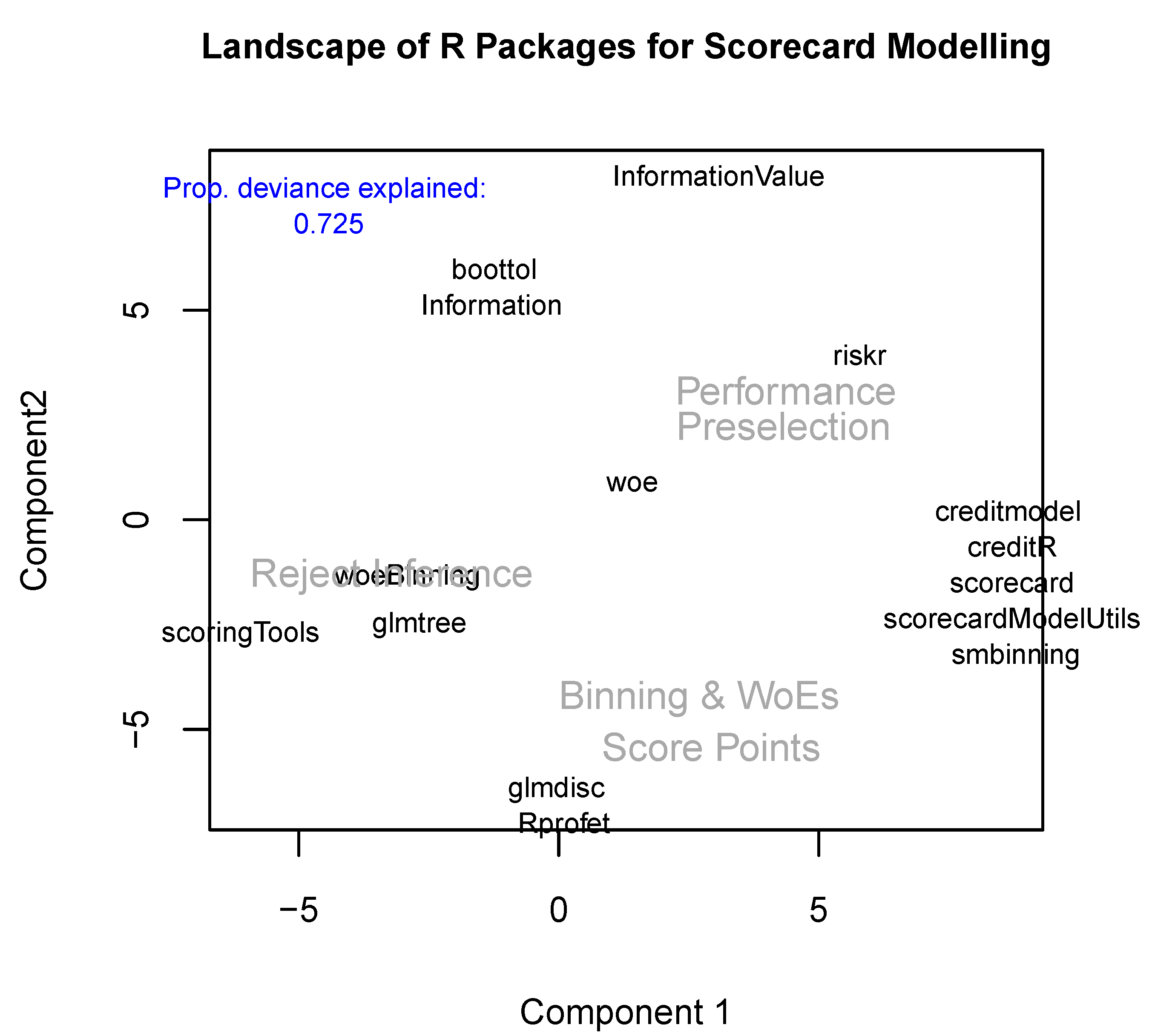
Finally, and with regard to the title of the paper, Figure 5 aims to visualize the ‘landscape’ of R packages dedicated to scorecard development using logistic principal component analysis (Landgraf and Lee 2015) as implemented in the logisticPCA package (Landgraf 2016) on the binary data given by Table 6.
The future will show to what degree the traditional process of credit risk scorecard development will stay as it is or whether or up to what extent the use of logistic regression will be replaced by more recent machine learning algorithms such as those offered by the recent powerful mlr3 framework in combination with explainable ML methodology to fulfill regulatory requirements (Bücker et al. 2021). The availability of open source frameworks for scorecard modelling as described above may help bridge the gap between academic advances in machine learning research and the traditional modelling process in the financial industry.

Funding

The APC was funded by Institute of Applied Computer Science, Stralsund.

Institutional Review Board Statement

Not applicable.

Informed Consent Statement

Not applicable.

Data Availability Statement

Reproducible code is available on the GitHub repository https://github.com/g-rho/CSwR (accessed on 15 February 2022).

Acknowledgments

Thanks to Rabea Aschenbruck and Alexander Frahm for support in writing this paper and to the forfunding of this work.

Conflicts of Interest

The author declares no conflict of interest.

Notes

1
2
3
4
5
https://github.com/ShichenXie/scorecardpy (accessed on 15 February 2022).
6
7
https://www.lendingclub.com/ (accessed on 15 February 2022).
8
Note that the package creditmodel supports a pos_flag to define the level of the positive class which currently does not work for Binning and Weights of Evidence.
9
Argument equal_bins = FALSE or initial bins of equal sample size otherwise.
10
An example code for the package riskr is given in Snippet 2 of the supplementary code.
11
An example using a lookup table for the variable purpose is given in Snippet 3 of the supplementary code.
12
A code example of looping through all (numeric) variables for the package smbinning is given in Snippet 4 of the supplementary code.
13
An example code for application of this mapping to new data is given in Snippet 5 of the supplementary code. The names of the resulting new levels are the concatenated old levels, separated by commas. Note that the function cannot deal with commas in the original level names: a new level <NA> will be assigned
14
Using method = “chimerge”.
15
Using best = TRUE.
16
This can be easily checked using the variable purpose, cf. e.g., Snippet 6 of the supplementary code.
17
A code snippet for creating a breaks_list (cf. above) from a binning result using the package woeBinning that can be imported for further use within the package scorecard, e.g., for manual manipulation of the bins is given by the function woeBins2breakslist() in Snippet 7 of the supplementary code
18
See footnote 10.
19
Note that the call of glmdisc() ran in an internal error (incorrect number of subscripts on matrix) for more than 10 iterations. For this reason the number of iterations has been reduced to 10 which is much smaller than the default of 1000 iterations and the reported Gini coefficient does still strongly vary among subsequent iterations. For larger numbers of iterations better results might have been possible.
20
Its argument data denotes the training data, output is a data frame with two variables specifying the variable names of the training data (character) and the corresponding cluster index, as given, e.g., by the result from variable.clustering(). Finally, its arguments variables and clusters denote the names of these two variables in the data frame from the output argument where the clustering results are stored.
21
A remedy how it can be used in combination with WoE assignment using the package klaR as shown in Example 4 is given in Snippet 9 of the supplementary code.
22
Snippet 10 of the supplementary code illustrates how the vector x of the names of the input variables in the original data frame can be extracted from the bicglm model after variable selection from Example 12.
23
For the function augmentation(), this is obtained by rounding the posterior probabilities to the first digit.
24
Here, the augmented weights within each score-band are computed by 1 + n r e j e c t e d n a c c e p t e d .
25
Within the function parcelling() this is done by sampling the labels from a binomial distribution.
26
As an exception, the package creditR has been developed as an extension of the package woeBinning.
27
Cf. corresponding footnotes in the paper. Supplementary code is available under https://github.com/g-rho/CSwR (accessed on 15 February 2022).

References

  1. Anagnostopoulos, Christoforos, and David J. Hand. 2019. Hmeasure: The H-Measure and Other Scalar Classification Performance Metrics, R Package Version 1.0-2; Available online: https://CRAN.R-project.org/package=hmeasure (accessed on 15 February 2022).
  2. Anderson, Raymond. 2007. The Credit Scoring Toolkit: Theory and Practice for Retail Credit Risk Management and Decision Automation. Oxford: Oxford University Press. [Google Scholar]
  3. Anderson, Raymond. 2019. Credit Intelligence & Modelling: Many Paths through the Forest. Oxford: Oxford University Press. [Google Scholar]
  4. Azevedo, Ana, and Manuel F. Santos. 2008. KDD, SEMMA and CRISP-DM: A parallel overview. Paper presented at IADIS European Conference on Data Mining 2008, Amsterdam, The Netherlands, July 24–26; pp. 182–85. [Google Scholar]
  5. Baesens, Bart, Tony Van Gestel, Stijn Viaene, Maria Stepanova, Johan Suykens, and Jan Vanthienen. 2002. Benchmarking state-of-the-art classification algorithms for credit scoring. JORS 54: 627–35. [Google Scholar] [CrossRef]
  6. Banasik, John, and Jonathan Crook. 2007. Reject inference, augmentation and sample selection. European Journal of Operational Research 183: 1582–94. [Google Scholar] [CrossRef] [Green Version]
  7. Biecek, Przemyslaw. 2018. DALEX: Explainers for complex predictive models. Journal of Machine Learning Research 19: 1–5. [Google Scholar]
  8. Binder, Martin, Florian Pfisterer, Michel Lang, Lennart Schneider, Lars Kotthoff, and Bernd Bischl. 2021. mlr3pipelines—Flexible machine learning pipelines in r. Journal of Machine Learning Research 22: 1–7. [Google Scholar]
  9. Bischl, Bernd, Martin Binder, Michel Lang, Tobias Pielok, Jakob Richter, Stefan Coors, Janek Thomas, Theresa Ullmann, Marc Becker, Anne-Laure Boulesteix, and et al. 2021. Hyperparameter optimization: Foundations, algorithms, best practices and open challenges. arXiv arXiv:2107.05847. [Google Scholar]
  10. Bischl, Bernd, Tobias Kühn, and Gero Szepannek. 2016. On class imbalance correction for classification algorithms in credit scoring. In Proceedings Operations Research 2014. Edited by Marco Lübbecke, Arie Koster, Peter Lethmathe, Reinhard Madlener, Britta Peis and Grit Walther. Heidelberg: Springer, pp. 37–43. [Google Scholar]
  11. Bischl, Bernd, Michel Lang, Lars Kotthoff, Julia Schiffner, Jakob Richter, Erich Studerus, Giuseppe Casalicchio, and Zachary Jones. 2016. mlr: Machine learning in R. Journal of Machine Learning Research 17: 1–5. [Google Scholar]
  12. Bischl, Bernd, Michel Lang, Lars Kotthoff, Patrick Schratz, Julia Schiffner, Jakob Richter, Zachary Jones, Giuseppe Casalicchio, Mason Gallo, Jakob Bossek, and et al. 2020. mlr: Machine Learning in R, R Package Version 2.17.1; Available online: https://CRAN.R-project.org/package=mlr (accessed on 15 February 2022).
  13. Bischl, Bernd, Olaf Mersmann, Heike Trautmann, and Claus Weihs. 2012. Resampling methods for meta-model validation with recommendations for evolutionary computation. Evolutionary Computation 20: 249–75. [Google Scholar] [CrossRef]
  14. Bravo, Cristian, Seppe van den Broucke, and Thomas Verbraken. 2019. EMP: Expected Maximum Profit Classification Performance Measure, R Package Version 2.0.5; Available online: https://CRAN.R-project.org/package=EMP (accessed on 15 February 2022).
  15. Breiman, Leo, Jerome H. Friedman, Richard A. Olshen, and Charles J. Stone. 1984. Classification and Regression Trees. New York: Wadsworth and Brooks. [Google Scholar]
  16. Brown, Iain, and Christophe Mues. 2012. An experimental comparison of classification algorithms for imbalanced credit scoring data sets. Expert Systems with Applications 39: 3446–53. [Google Scholar] [CrossRef] [Green Version]
  17. Bücker, Michael, Maarten van Kampen, and Walter Krämer. 2013. Reject inference in consumer credit scoring with nonignorable missing data. Journal of Banking & Finance 37: 1040–45. [Google Scholar]
  18. Bücker, Michael, Gero Szepannek, Alicja Gosiewska, and Przemyslaw Biecek. 2021. Transparency, Auditability and explainability of machine learning models in credit scoring. Journal of the Operational Research Society 73: 1–21. [Google Scholar] [CrossRef]
  19. Chavent, Marie, Vanessa Kuentz, Benoit Liquet, and Jerome Saracco. 2017. ClustOfVar: Clustering of Variables, R Package Version 1.1; Available online: https://CRAN.R-project.org/package=ClustOfVar (accessed on 15 February 2022).
  20. Chavent, Marie, Vanessa Kuentz-Simonet, Benoît Liquet, and Jerome Saracco. 2012. Clustofvar: An r package for the clustering of variables. Journal of Statistical Software 50: 1–6. [Google Scholar] [CrossRef] [Green Version]
  21. Chawla, Nitesh V., Kevin W. Bowyer, Lawrence O. Hall, and W. Philip Kegelmeyer. 2002. Smote: Synthetic minority over-sampling technique. Journal of Artificial Intelligence Research 16: 321–57. [Google Scholar] [CrossRef]
  22. Chen, Chaofan, Kangcheng Lin, Cynthia Rudin, Yaron Shaposhnik, Sijia Wang, and Tong Wang. 2018. An interpretable model with globally consistent explanations for credit risk. arXiv arXiv:1811.12615. [Google Scholar]
  23. Chen, Tianqi, and Carlos Guestrin. 2016. Xgboost: A scalable tree boosting system. Paper presented at the 22nd ACM SIGKDD International Conference on Knowledge Discovery and Data Mining, San Francisco, CA, USA, August 13–17; pp. 785–94. [Google Scholar] [CrossRef] [Green Version]
  24. Chen, Tianqi, Tong He, Michael Benesty, Vadim Khotilovich, Yuan Tang, Hyunsu Cho, Kailong Chen, Rory Mitchell, Ignacio Cano, Tianyi Zhou, and et al. 2021. xgboost: Extreme Gradient Boosting, R Package Version 1.5.0.2; Available online: https://CRAN.R-project.org/package=xgboost (accessed on 15 February 2022).
  25. Cordón, Ignacio, Salvador García, Alberto Fernández, and Francisco Herrera. 2018. Imbalance: Oversampling algorithms for imbalanced classification in r. Knowledge-Based Systems 161: 329–41. [Google Scholar] [CrossRef]
  26. Cordón, Ignacio, Salvador García, Alberto Fernández, and Francisco Herrera. 2020. imbalance: Preprocessing Algorithms for Imbalanced Datasets, R Package Version 1.0.2.1; Available online: https://CRAN.R-project.org/package=imbalance (accessed on 15 February 2022).
  27. Crone, Sven F., and Steven Finlay. 2012. Instance sampling in credit scoring: An empirical study of sample size and balancing. International Journal of Forecasting 28: 224–38. [Google Scholar] [CrossRef]
  28. Crook, Jonathan, and John Banasik. 2004. Does reject inference really improve the performance of application scoring models? Journal of Banking & Finance 28: 857–74. [Google Scholar] [CrossRef] [Green Version]
  29. Csárdi, Gábor. 2019. cranlogs: Download Logs from the ’RStudio’ ’CRAN’ Mirror, R Package Version 2.1.1; Available online: https://CRAN.R-project.org/package=cranlogs (accessed on 15 February 2022).
  30. DeLong, Elizabeth R., David M. DeLong, and Daniel L. Clarke-Pearson. 1988. Comparing the areas under two or more correlated receiver operating characteristic curves: A nonparametric approach. Biometrics 44: 837–45. [Google Scholar] [CrossRef]
  31. Dis, Ayhan. 2020. creditR: A Credit Risk Scoring and Validation Package, R Package Version 0.1.0; Available online: https://github.com/ayhandis/creditR (accessed on 15 February 2022).
  32. Dua, Dheeru, and Casey Graff. 2019. UCI Machine Learning Repository. Irvine: University of California. [Google Scholar]
  33. Ehrhardt, Adrien. 2018. scoringTools: Credit Scoring Tools, R Package Version 0.1; Available online: https://CRAN.R-project.org/package=scoringTools (accessed on 15 February 2022).
  34. Ehrhardt, Adrien. 2020. glmtree: Logistic Regression Trees, R Package Version 0.2; Available online: https://CRAN.R-project.org/package=glmtree (accessed on 15 February 2022).
  35. Ehrhardt, Adrien, Christophe Biernacki, Vincent Vandewalle, and Philippe Heinrich. 2019. Feature quantization for parsimonious and interpretable predictive models. arXiv arXiv:1903.08920. [Google Scholar]
  36. Ehrhardt, Adrien, Christophe Biernacki, Vincent Vandewalle, Philippe Heinrich, and Sébastien Beben. 2019. Réintégration des refusés en credit scoring. arXiv arXiv:1903.10855. [Google Scholar]
  37. Ehrhardt, Adrien, and Vincent Vandewalle. 2020. glmdisc: Discretization and Grouping for Logistic Regression, R Package Version 0.6; Available online: https://CRAN.R-project.org/package=glmdisc (accessed on 15 February 2022).
  38. Eichenberg, Thilo. 2018. woeBinning: Supervised Weight of Evidence Binning of Numeric Variables and Factors, R Package Version 0.1.6; Available online: https://CRAN.R-project.org/package=woeBinning (accessed on 15 February 2022).
  39. Fan, Dongping. 2022. creditmodel Toolkit for Credit Modeling, Analysis and Visualization, R Package Version 1.3.1; Available online: https://CRAN.R-project.org/package=creditmodel (accessed on 15 February 2022).
  40. Financial Stability Board. 2017. Artificial Intelligence and Machine Learning in Financial Services—Market Developments and Financial Stability Implications. Available online: https://www.fsb.org/2017/11/artificial-intelligence-and-machine-learning-in-financial-service/ (accessed on 15 February 2022).
  41. Finlay, Steven. 2012. Credit Scoring, Response Modelling and Insurance Rating. London: Palgarve MacMillan. [Google Scholar]
  42. Fox, John, and Sanford Weisberg. 2019. An R Companion to Applied Regression, 3rd ed. Thousand Oaks: Sage. [Google Scholar]
  43. Fox, John, Sanford Weisberg, Brad Price, Daniel Adler, Douglas Bates, Gabriel Baud-Bovy, Ben Bolker, Steve Ellison, David Firth, Michael Friendly, and et al. 2021. car: Companion to Applied Regression, R Package Version 3.0-12; Available online: https://CRAN.R-project.org/package=car (accessed on 15 February 2022).
  44. Goodman, Bryce, and Seth Flaxman. 2017. European union regulations on algorithmic decision-making and a “right to explanation”. AI Magazine 38: 50–57. [Google Scholar] [CrossRef] [Green Version]
  45. Greenwell, Brandon, Bradley Boehmke, Jay Cunningham, and GBM Developers. 2020. gbm: Generalized Boosted Regression Models, R Package Version 2.1.8; Available online: https://CRAN.R-project.org/package=gbm (accessed on 15 February 2022).
  46. Groemping, Ulrike. 2019. South German Credit Data: Correcting a Widely Used Data Set. Technical Report 4/2019. Berlin: Department II, Beuth University of Applied Sciences Berlin. [Google Scholar]
  47. Hand, David. 2009. Measuring classifier performance: A coherent alternative to the area under the roc curve. Machine Learning 77: 103–23. [Google Scholar] [CrossRef] [Green Version]
  48. Hand, David, and William Henley. 1993. Can reject inference ever work? IMA Journal of Management Matehmatics 5: 45–55. [Google Scholar] [CrossRef]
  49. Hastie, Trevor, Robert Tibshirani, and Jerome Friedman. 2009. The Elements of Statistical Learning, 2nd ed. New York: Springer. [Google Scholar]
  50. Hoffmann, Hans. 1994. German Credit Data Set (statlog). Available online: https://archive.ics.uci.edu/ml/datasets/statlog+(german+credit+data) (accessed on 15 February 2022).
  51. Hosmer, David W., and Stanley Lemeshow. 2000. Applied Logistic Regression. Hoboken: Wiley. [Google Scholar]
  52. Hothorn, Thorsten, Kurt Hornik, and Achim Zeileis. 2006. Unbiased recursive partitioning: A conditional inference framework. Journal of Computational and Graphical Statistics 15: 651–74. [Google Scholar] [CrossRef] [Green Version]
  53. Hothorn, Torsten, and Achim Zeileis. 2015. partykit: A modular toolkit for recursive partytioning in R. Journal of Machine Learning Research 16: 3905–9. [Google Scholar]
  54. Izrailev, Sergei. 2015. Binr: Cut Numeric Values into Evenly Distributed Groups, R Package Version 1.1; Available online: https://CRAN.R-project.org/package=binr (accessed on 15 February 2022).
  55. Jopia, Herman. 2019. smbinning: Optimal Binning for Scoring Modeling, R Package Version 0.9; Available online: https://CRAN.Rproject.org/package=smbinning (accessed on 15 February 2022).
  56. Kaszynski, Daniel. 2020. Background of credit scoring. In Credit Scoring in Context of Interpretable Machine Learning. Edited by Daniel Kaszynski, Bogumil Kaminski and Tomasz Szapiro. Warsaw: SGH, pp. 17–26. [Google Scholar]
  57. Kaszynski, Daniel, Bogumil Kaminski, and Tomasz Szapiro. 2020. Credit Scoring in Context of Interpretable Machine Learning. Warsaw: SGH. [Google Scholar]
  58. Kim, HyunJi. 2012. Discretization: Data Preprocessing, Discretization for Classification, R Package Version 1.0-1; Available online: https://CRAN.R-project.org/package=discretization (accessed on 15 February 2022).
  59. Kuhn, Max. 2008. Building predictive models in r using the caret package. Journal of Statistical Software 28: 1–26. [Google Scholar] [CrossRef] [Green Version]
  60. Kuhn, Max. 2021. Caret: Classification and Regression Training, R Package Version 6.0-90; Available online: https://CRAN.R-project.org/package=caret (accessed on 15 February 2022).
  61. Kunst, Joshua. 2020. Riskr: Functions to Facilitate the Evaluation, Monitoring and Modeling process, R Package Version 1.0; Available online: https://github.com/jbkunst/riskr (accessed on 15 February 2022).
  62. Landgraf, Andrew J. 2016. logisticPCA: Binary Dimensionality Reduction, R Package Version 0.2; Available online: https://CRAN.Rproject.org/package=logisticPCA (accessed on 15 February 2022).
  63. Landgraf, Andrew J., and Yoonkyung Lee. 2015. Dimensionality reduction for binary data through the projection of natural parameters. arXiv arXiv:1510.06112. [Google Scholar] [CrossRef]
  64. Lang, Michel, Martin Binder, Jakob Richter, Patrick Schratz, Florian Pfisterer, Stefan Coors, Quay Au, Giuseppe Casalicchio, Lars Kotthoff, and Bernd Bischl. 2019. mlr3: A modern object-oriented machine learning framework in R. Journal of Open Source Software 4: 1903. [Google Scholar] [CrossRef] [Green Version]
  65. Lang, Michel, Bernd Bischl, Jakob Richter, Patrick Schratz, Giuseppe Casalicchio, Stefan Coors, Quay Au, and Martin Binder. 2021. mlr3: Machine Learning in R—Next Generation, R Package Version 0.13.0; Available online: https://CRAN.R-project.org/package=mlr3 (accessed on 15 February 2022).
  66. Larsen, Kim. 2016. Information: Data Exploration with Information Theory, R Package Version 0.0.9; Available online: https://CRAN.R-project.org/package=Information (accessed on 15 February 2022).
  67. Lele, Subhash R., Jonah L. Keim, and Peter Solymos. 2019. ResourceSelection: Resource Selection (Probability) Functions for Use-Availability Data, R Package Version 0.3-5; Available online: https://CRAN.R-project.org/package=ResourceSelection (accessed on 15 February 2022).
  68. Lessmann, Stefan, Bart Baesens, Hsin-Vonn Seow, and Lyn Thomas. 2015. Benchmarking state-of-the-art classification algorithms for credit scoring: An update of research. European Journal of Operational Research 247: 124–36. [Google Scholar] [CrossRef] [Green Version]
  69. Liaw, Andy, and Matthew Wiener. 2002. Classification and regression by randomforest. R News 2: 18–22. [Google Scholar]
  70. Ligges, Uwe. 2009. Programmieren Mit R, 3rd ed. Heidelberg: Springer. [Google Scholar]
  71. Little, Roderick, and Donald Rubin. 2002. Statistical Analysis with Missing Data. Hoboken: Wiley. [Google Scholar]
  72. Louzada, Francisco, Anderson Ara, and Guilherme Fernandes. 2016. Classification methods applied to credit scoring: A systematic review and overall comparison. Surveys in OR and Management Science 21: 117–34. [Google Scholar] [CrossRef] [Green Version]
  73. Maechler, Martin, Peter Rousseeuw, Anja Struyf, Mia Hubert, and Kurt Hornik. 2021. Cluster: Cluster Analysis Basics and Extensions, R Package Version 2.1.2; Available online: https://CRAN.R-project.org/package=cluster (accessed on 15 February 2022).
  74. Molnar, Christoph, Bernd Bischl, and Giuseppe Casalicchio. 2018. iml: An R package for Interpretable Machine Learning. JOSS 3: 786. [Google Scholar] [CrossRef] [Green Version]
  75. Paradis, Emmanuel, Simon Blomberg, Ben Bolker, Joseph Brown, Julien Claude, Hoa Sien Cuong, Richard Desper, Gilles Didier, Benoit Durand, Julien Dutheil, and et al. 2021. ape: Analyses of Phylogenetics and Evolution, R Package Version 5.6.1; Available online: https://CRAN.R-project.org/package=ape (accessed on 15 February 2022).
  76. Paradis, Emmanuel, and Klaus Schliep. 2018. ape 5.0: An environment for modern phylogenetics and evolutionary analyses in R. Bioinformatics 35: 526–28. [Google Scholar] [CrossRef]
  77. Poddar, Arya. 2019. scorecardModelUtils: Credit Scorecard Modelling Utils, R Package Version 0.0.1.0; Available online: https://CRAN.R-project.org/package=scorecardModelUtils (accessed on 15 February 2022).
  78. Pozzolo, Andrea Dal, Olivier Caelen, and Gianluca Bontempi. 2015. unbalanced: Racing for Unbalanced Methods Selection, R Package Version 2.0; Available online: https://CRAN.R-project.org/package=unbalanced (accessed on 15 February 2022).
  79. Prabhakaran, Selva. 2016. InformationValue: Performance Analysis and Companion Functions for Binary Classification Models, R Package Version 1.2.3; Available online: https://CRAN.R-project.org/package=InformationValue (accessed on 15 February 2022).
  80. Robin, Xavier, Natacha Turck, Alexandre Hainard, Natalie Tiberti, Frederique Lisacek, Jean Sanchez, and Markus Müller. 2011. Proc: An open-source package for r and s+ to analyze and compare roc curves. BMC Bioinformatics 12: 1–8. [Google Scholar] [CrossRef]
  81. Robin, Xavier, Natacha Turck, Alexandre Hainard, Natalia Tiberti, Frederique Lisacek, Jean-Charles Sanchez, Markus Müller, Stefan Siegert, and Matthias Doering. 2021. pROC: Display and Analyze ROC Curves, R Package Version 1.18.0; Available online: https://CRAN.R-project.org/package=pROC (accessed on 15 February 2022).
  82. Roever, Christian, Nils Raabe, Karsten Luebke, Uwe Ligges, Gero Szepannek, and Marc Zentgraf. 2020. klaR: Classification and visualization, R Package Version 0.6-15; Available online: https://CRAN.R-project.org/package=klaR (accessed on 15 February 2022).
  83. Rudin, Cynthia. 2019. Stop explaining black box machine learning models for high stakes decisions and use interpretable models instead. Nature Machine Intelligence 1: 206–15. [Google Scholar] [CrossRef] [Green Version]
  84. Ryu, Choonghyun. 2021. dlookr: Tools for Data Diagnosis, Exploration, Transformation, R Package Version 0.5.4; Available online: https://CRAN.R-project.org/package=dlookr (accessed on 15 February 2022).
  85. Scallan, Gerard. 2011. Class(ic) scorecards—Selecting attributes in logistic regression. Credit Scoring and Credit Control XIII. Available online: https://www.scoreplus.com/papers/paper (accessed on 15 February 2022).
  86. Schiltgen, Garrett. 2015. Boottol: Bootstrap Tolerance Levels for Credit Scoring Validation Statistics, R Package Version 2.0; Available online: https://CRAN.R-project.org/package=boottol (accessed on 15 February 2022).
  87. Sharma, Dhuv. 2009. Guide to credit scoring in R. CRAN Documentation Contribution. Available online: https://cran.r-project.org/ (accessed on 15 February 2022).
  88. Siddiqi, Naeem. 2006. Credit Risk Scorecards: Developing and Implementing Intelligent Credit Scoring, 2nd ed. Hoboken: Wiley. [Google Scholar]
  89. Sing, Tobias, Oliver Sander, Niko Beerenwinkel, and Thomas Lengauer. 2005. ROCR: Visualizing classifier performance in R. Bioinformatics 21: 7881. [Google Scholar] [CrossRef]
  90. Sing, Tobias, Oliver Sander, Niko Beerenwinkel, and Thomas Lengauer. 2020. ROCR: Visualizing the Performance of Scoring Classifiers, R Package Version 1.0-11; Available online: https://CRAN.R-project.org/package=ROCR (accessed on 15 February 2022).
  91. Siriseriwan, Wacharasak. 2019. smotefamily: A Collection of Oversampling Techniques for Class Imbalance Problem Based on SMOTE, R Package Version 1.3.1; Available online: https://CRAN.R-project.org/package=smotefamily (accessed on 15 February 2022).
  92. Staniak, Mateusz, and Przemysław Biecek. 2019. The Landscape of R Packages for Automated Exploratory Data Analysis. The R Journal 11: 347–69. [Google Scholar] [CrossRef]
  93. Stratman, Eric, Riaz Khan, and Allison Lempola. 2020. Rprofet: WOE Transformation and Scorecard Builder, R Package Version 2.2.1; Available online: https://CRAN.R-project.org/package=Rprofet (accessed on 15 February 2022).
  94. Sun, Xu, and Weichao Xu. 2014. Fast implementation of delong’s algorithm for comparing the areas under correlated receiver operating characteristic curves. IEEE Signal Processing Letters 21: 1389–93. [Google Scholar] [CrossRef]
  95. Szepannek, Gero. 2017. On the practical relevance of modern machine learning algorithms for credit scoring applications. WIAS Report Series 29: 88–96. [Google Scholar]
  96. Szepannek, Gero. 2019. How much can we see? A note on quantifying explainability of machine learning models. arXiv arXiv:1910.13376. [Google Scholar]
  97. Szepannek, Gero, and Karsten Lübke. 2021. Facing the challenges of developing fair risk scoring models. Frontiers in Artificial Intelligence 4: 117. [Google Scholar] [CrossRef] [PubMed]
  98. Therneau, Terry, and Beth Atkinson. 2019. rpart: Recursive Partitioning and Regression Trees, R Package Version 4.1-15; Available online: https://CRAN.R-project.org/package=rpart (accessed on 15 February 2022).
  99. Thomas, Lynn C., Jonathan N. Crook, and David B. Edelman. 2019. Credit Scoring and its Applications, 2nd ed. Philadelphia: SIAM. [Google Scholar]
  100. Thoppay, Sudarson. 2015. woe: Computes Weight of Evidence and Information Values, R Package Version 0.2; Available online: https://CRAN.R-project.org/package=woe (accessed on 15 February 2022).
  101. Verbraken, Thomas, Christian Bravo, Weber Richard, and Baesens Baesens. 2014. Development and application of consumer credit scoring models using profit-based classification measures. European Journal of Operational Research 238: 505–13. [Google Scholar] [CrossRef] [Green Version]
  102. Verstraeten, Geert, and Dirk Van den Poel. 2005. The impact of sample bias on consumer credit scoring performance and profitability. JORS 56: 981–92. [Google Scholar] [CrossRef]
  103. Vigneau, Evelyne, Mingkun Chen, and Veronique Cariou. 2020. ClustVarLV: Clustering of Variables Around Latent Variables, R Package Version 2.0.1; Available online: https://CRAN.R-project.org/package=ClustVarLV (accessed on 15 February 2022).
  104. Vigneau, Evelyne, Mingkun Chen, and El Mostafa Qannari. 2015. ClustVarLV: An R Package for the Clustering of Variables Around Latent Variables. The R Journal 7: 134–48. [Google Scholar] [CrossRef] [Green Version]
  105. Vincotti, Veronica, and David Hand. 2002. Scorecard construction with unbalanced class sizes. Journal of The Iranian Statistical Society 2: 189–205. [Google Scholar]
  106. Wrzosek, Malgorzata, Daniel Kaszynski, Karol Przanowski, and Sebastian Zajac. 2020. Selected machine learning methods used for credit scoring. In Credit Scoring in Context of Interpretable Machine Learning. Edited by Daniel Kaszynski, Bogumil Kaminski and Tomasz Szapiro. Warsaw: SGH, pp. 83–146. [Google Scholar]
  107. Xie, Shichen. 2021. scorecard: Credit Risk Scorecard, R Package Version 0.3.6; Available online: https://CRAN.R-project.org/package=scorecard (accessed on 15 February 2022).
  108. Zumel, Nina, and John Mount. 2014. Practical Data Science with R. New York: Manning. [Google Scholar]
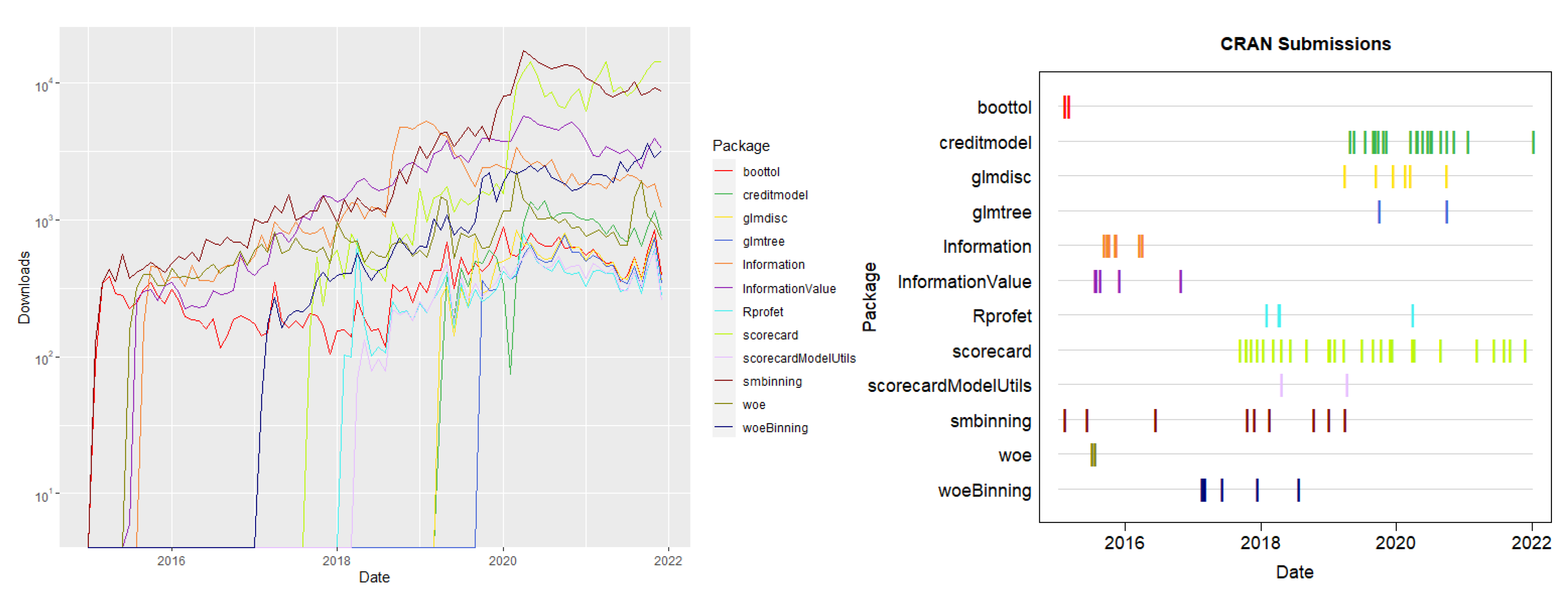
Figure 1. CRAN release activity and download statistics (as returned by cranlogs, Csárdi 2019) of packages available on CRAN.
Risks 10 00067 g001
Figure 2. Visualization of the bins for the variable purpose as created by the package scorecard (left) and mosaicplot of the binning result by the package glmdisc (right).
Risks 10 00067 g002
Figure 3. Reordered correlation matrix (left) and phylogenetic tree of the clustered variables (right).
Risks 10 00067 g003
Figure 4. Scorecard performance graphs: ECDF (top left); score densities (top right); gains (bottom left); ROC (bottom right).
Risks 10 00067 g004
Figure 5. Landscape of R packages for scorecard modelling using logistic PCA.
Risks 10 00067 g005
Table 1. Number of bins after automatic binning. Abbreviations of package names: sc = scorecard; woeB = woeBinning using woe.binning(); woeB.T = woeBinning using woe.tree.binning(); sMU = scorecardModelUtils; Rprof = Rprofet; smb = smbinning and cremo = creditmodel.
UniquescwoeBwoeB.TGlmdiscsMURprofsmbCremoRiskr
Avg. # bins 6.334.3362.673.67112.6722.67
duration325553513323
amount6637461311323
instRate4444144421
residence4444324431
age52747439222
numCredits4233223421
numLiable2233212221
Table 2. Gini coefficient of WoE transformed variables on validation data.
LCLscwoeBwoeB.TGlmdiscsMUsmbCremoRiskr
duration0.1700.2970.2590.2640.2650.2990.2480.1620.248
amount0.1160.2510.1790.2270.0000.1960.2190.0690.219
age0.0780.1790.1690.2220.1890.2000.187−0.0030.187
numLiable0.0000.0060.0060.0060.0060.0000.0060.0060.000
numCredits0.0000.0680.0680.0680.0680.0680.0610.0680.000
residence0.0000.0060.0170.0170.0170.0290.0060.0170.000
instRate0.0000.1080.1030.1030.0000.1080.1080.1040.000
Table 3. Summary of the functionalities for binning and WoEs provided by the different packages where ✓ denotes available and ✗ not available. An empty field means that this is not relevant w.r.t. the scope of the package. (1): workaround available (cf. above); (2) separate bin (00.NA) is created—binning of new data (split_bins_all()) possible but no WoE assignment ((woe_trans_all)); (3) always bin 1 assigned; (4) separate function missing_val() for imputation; (5) additional function cat_to_new() merges levels smaller than threshold (cf. above).
scsmbwoeBCremoRiskrGlmdiscsMURprofklaR
automatic binning of numerics
automatic binning of factors
store and predict numerics(1)
store and predict factors(1)
supports bin prediction(1)
supports WoE prediction
summary table
plot
manual modification
multiple variables
supported target levels
adjust WoEs
NAs(2)(3)(4)
new levels (3)
level order irrelevant
min. level size (5)
Table 4. Packages and functions for computation of IVs.
PackageFunctionTarget TypeMultiple VariablesWoE Adjustment
creditRIV.calc.data()both, levels 0/1yesno
creditmodelget_iv_all()both, levels 0/1yesyes
Informationcreate_infotables()numeric 0/1yesyes
InformationValueIV()numeric 0/1noyes
klaRwoe()factoryesargument
riskrpred_ranking()numeric 0/1yesno
scorecardiv()bothyes0.99
scorecardModelUtilsiv_table()numeric 0/1yes0.5
smbinningsmbinning.sumiv()numeric 0/1yesyes
Table 5. Overview of scorecard performance summary functions.
Package FunctionRiskrPerf()ScorecardPerf_Eva()ScorecardModelUtilsGini_Table()SmbinningSmbinning.Metrics()
KS
AUC
Gini
Divergence
Bin table
Confusion matrix
Accuracy
Good rate
Bad rate
TPR
FNR
TNR
FPR
PPV
FDR
FOR
NPV
ROC curve
Score densities | y
ECDF
Gain chart
Table 6. Overview of R packages with the explicit scope of scorecard modelling and addressed stages of the development process.
PackageBinning & WoEsPreselectionScorecardPerformanceReject Inference
boottol
creditmodel
creditR
glmdisc
glmtree
Information
InformationValue
riskr
Rprofet
scorecard
scoringTools
scorecardModelUtils
smbinning
woe
woeBinning
Publisher’s Note: MDPI stays neutral with regard to jurisdictional claims in published maps and institutional affiliations.