Review

Stochastic and Temporal Models of Olfactory Perception

by
Thomas P. Hettinger
and
Marion E. Frank
*
Dental Medicine, UConn Health, 263 Farmington Ave., Farmington, CT 06030, USA
*
Author to whom correspondence should be addressed.
Chemosensors 2018, 6(4), 44; https://doi.org/10.3390/chemosensors6040044
Submission received: 3 August 2018 / Revised: 5 September 2018 / Accepted: 18 September 2018 / Published: 26 September 2018
(This article belongs to the Special Issue Electronic nose’s, Machine Olfaction and Electronic Tongue’s)

Abstract

:
Olfactory systems typically process signals produced by mixtures composed of very many natural odors, some that can be elicited by single compounds. The several hundred different olfactory receptors aided by several dozen different taste receptors are sufficient to define our complex chemosensory world. However, sensory processing by selective adaptation and mixture suppression leaves only a few perceptual components recognized at any time. Thresholds determined by stochastic processes are described by functions relating stimulus detection to concentration. Relative saliences of mixture components are established by relating component recognition to concentration in the presence of background components. Mathematically distinct stochastic models of perceptual component dominance in binary mixtures were developed that accommodate prediction of an appropriate range of probabilities from 0 to 1, and include errors in identifications. Prior short-term selective adaptation to some components allows temporally emergent recognition of non-adapted mixture-suppressed components. Thus, broadly tuned receptors are neutralized or suppressed by activation of other more efficacious receptors. This ‘combinatorial’ coding is more a process of subtraction than addition, with the more intense components dominating the perception. It is in this way that complex chemosensory mixtures are reduced to manageable numbers of odor notes and taste qualities.

1. Introduction

1.1. Preamble

This article presents an emerging view of odor coding in humans. It developed from consideration of diverse topics such as odor chemistry, olfactory and gustatory receptors, neural processing, adaptation, mixture suppression, and human perception of odors and tastes. In particular, we are not claiming a definitive answer to all aspects of odor coding, but presenting a point of view that we think should be considered in any treatment of odor coding. Though we are mostly focused on perception of odor quality, the above factors must be considered before we elaborate on our main topics of perception of mixtures in Section 2, selective adaptation in Section 3, and models of component interaction in Section 4.

1.2. Odor Identification of Single Compounds

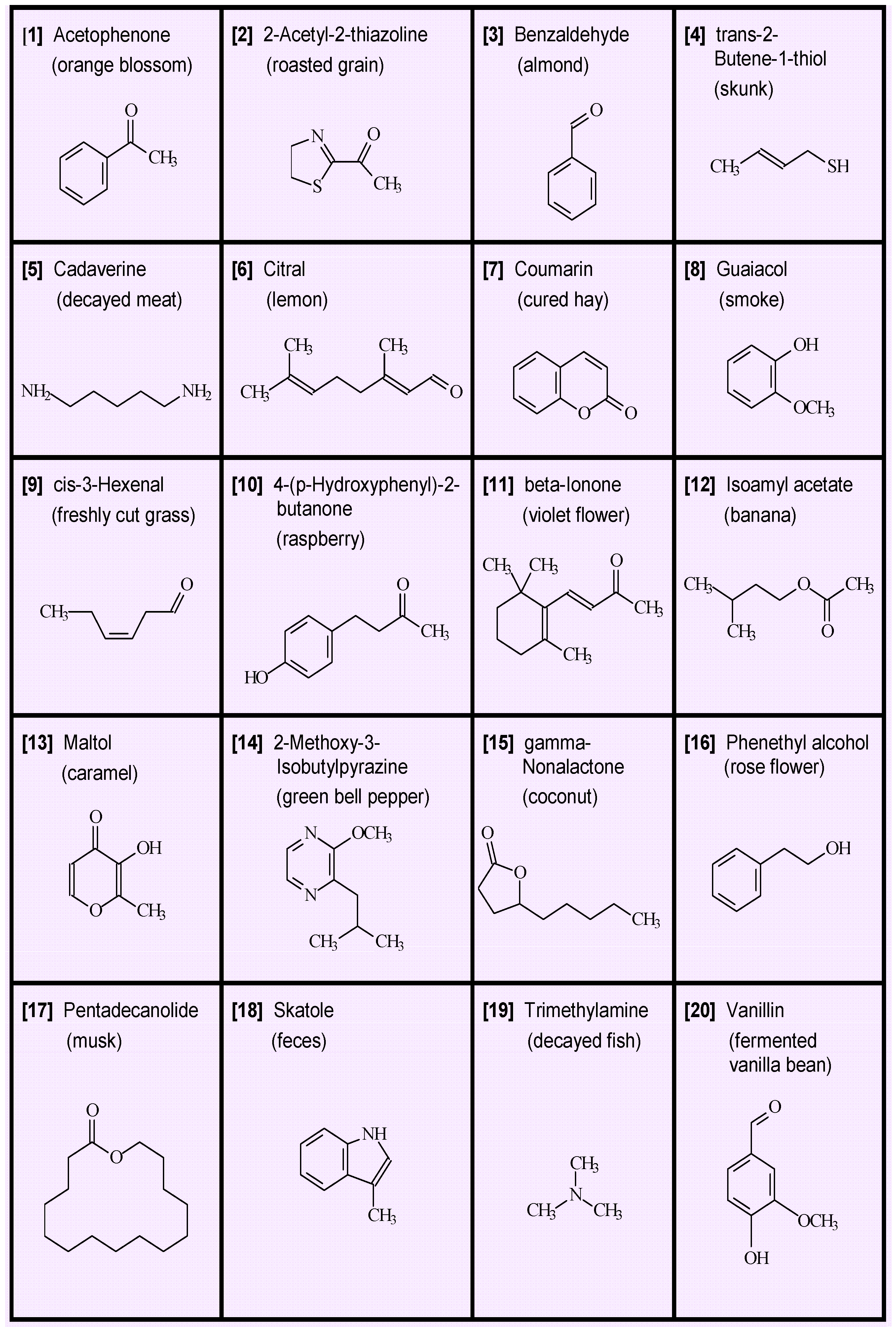
  • Single odors. Perhaps the most straightforward aspect of smell is odor identification, which generally attaches a name or label to an odor object. There are, nevertheless, challenges in naming odors because odor objects are not always completely defined and because subjects may have different perceptions and experiences. A key observation that has been made numerous times in the history of odor chemistry is that many natural odors can be imitated by a single chemical substance. We present in Figure 1 an array of 20 diverse chemicals that by themselves epitomize a characteristic odor object [1]. For example, single compounds such as vanillin convey a pleasant food odor but a decayed odor is conveyed by cadaverine. We note that in the case of the latter compound, numerous metabolic decomposition products can be present, but odor of decay can be represented by a single chemical [2].
  • Number of odorants in single odor objects. The natural environment is replete with numerous odors, but most of the time we are not aware of any odors. This is partly due to the effect of adaptation, but it is also due to the great dilution of odors compared to the concentration at their source. Even here, we should recognize that flowers are most often associated with the idea of odor, yet flowers are often completely odorless. If half of all flowers are odorless, we can speculate on the chemical composition of odorants in flowers that have odors. We would not expect nature to pack many odorants into some flowers and none in others. Suppose there were just eight possible odorants, and a given flower had an 8% chance of producing each odorant, then the probability that the flower would be odorless is 0.928, or about 51% by chance. In this assumed situation, about 49% of flowers would have an odor and binomial calculations show about 73% of them would have one odorant, about 22% would have two odorants, and about 4% would have three odorants. Similar results are obtained for a larger number of potential odorants and a correspondingly lower chance occurrence per odorant. The conclusion would be the odor of the majority of flowers is due to a single component, and only about 1% is due to more than three components. This argument can be extended to other sources of odor than flowers, but with less certainty.
  • Few odors dominate perception. The sparse existence of odorants in the environment and in odor objects in general is a concept at odds with accepted views of olfaction. Many articles repeat the refrain that objects such as coffee or grilled meat contain hundreds of odorants that act in a combinatorial way to produce their characteristic odors. While it is true that many odorants are present, they are mostly present at concentrations below threshold and therefore contribute little or nothing to the overall odor. Odorants are present at widely different perceptual intensities, with the strongest odors dominating the perception. In the paper by Bushdid et al. [3], the calculation of the possibility of a trillion distinguishable odors was based in part on the use of artificial mixtures of as many as 30 components that were presumed to be equally intense. Such a situation is unrealistic and difficult to achieve. If there was an imbalance in intensity of the components, the calculated value could be too large by many orders of magnitude. In simple binary mixtures, the dominance of one component over the other is achieved when the intensities of the components differ by a factor of more than 1.4. An extensive discussion of the perception of binary mixtures is presented in Section 2.

1.3. Chemical Identification and Purity

The identification of natural odor chemicals is not straightforward. Natural odor objects are often composed of numerous odorants at widely different concentrations and can have very different odor intensities. When components are separated by gas chromatography (GC), the measured size of the GC peak may not relate easily to odor intensity. Identification of peaks by mass spectrometry (MS) has to consider that the main MS peak will be the same for different isomers with different odors. Odors are often evident in GC bands even when peaks are practically non-existent. The odors of GC bands may not correspond to odors of ostensibly pure chemicals obtained by chemical suppliers. This is because impurities can have more intense odors than the main component. There are many examples in the literature where either the chemical was misidentified or the odor was inaccurate.

1.4. Odor Intensity

  • Stevens’ power law, subjective and no threshold. After chemical components of odor objects are properly identified, it is essential to determine the relative intensities or salience of the components. In the sensory psychology literature, the perceptual intensity of an odorant is generally estimated from Stevens’ power law, which states that intensity (I) is a power function of concentration (C) such that I = kC a , where k is a constant and the exponent (a) can vary between about 0.1 and 1, depending on the odorant and conditions of measurement. An exponent below 1 is interpreted to mean that perceptual intensity is a ‘compressed’ function of concentration. In our treatment, we assume that the typical value of the exponent is approximately 0.5, that is, the odor intensity is proportional to the square root of the concentration ( I = k C ). A problem with the Stevens’ power law is the need for the subject to make what is essentially a subjective estimate of intensity by the method of magnitude estimation. Also, the power law does not provide an absolute reference point for intensity and does not establish a threshold value.
  • Odor activity value, stimulus/threshold concentrations. A way around these problems is to establish a reasonably objective measurement of threshold and then to infer relative stimulus intensity from the ratio of suprathreshold concentration (C) to threshold concentration (T). In the food and fragrance literature, this ratio (C/T) is called the odor activity value (OAV) [4]. The OAV is not equal to perceptual intensity (I), but a mathematical relationship can be established as follows: Because I = k C and I ( threshold ) = k T , then I / I ( threshold ) = OAV . Thus, the ratio of perceived odor intensity to its intensity at threshold is approximately equal to the square root of the odor activity value. This relationship will be used later in the treatment of perception of mixtures (Section 2) and development of stochastic models (Section 4).

1.5. Threshold Determination

Many different methods have been used to determine odor thresholds. Some use direct measurement of odorant concentration in the gas phase, whereas others infer a threshold by detection of odorant in the headspace above a known concentration of odorant in a liquid such as water or propylene glycol. Ascending and descending concentrations are used in the method of limits where reversals attain an asymptotic threshold. Psychometric methods using detection probability as a function of concentration [5] are currently thought to be the most precise. Threshold is defined as the concentration giving correct identification halfway between chance and perfect performance. In methods of analysis of complex natural mixtures by gas chromatography, a simple method of serial dilution is used to establish a threshold, which is defined as the highest dilution where the odorant can be detected. Because this method is labor-intensive and tedious, thresholds are generally accurate only by a factor of 2. The odor activity value of an odorant is the ratio of the concentration in the sample to the threshold concentration [4].

1.6. Receptor Mechanisms

  • Numbers of receptors. Chemosensory receptors for taste and smell have distinctly different chemistries (Table 1). Humans have about 390 types of functional olfactory receptors and only about 34 types of taste receptors, most of which serve to detect bitter stimuli.
  • Combinatorial odor coding. In developing the combinatorial concept for receptor activation for odors, Malnic et al. [6] found that receptors appeared to be broadly tuned and that many odorants activated multiple receptors. This may be the case when relatively high concentrations of odorants in the range of 10 to 100 micromolar are used. Some stimuli having little volatility and no odor, such as dicarboxylic acids, were used in developing the combinatorial theory. At much lower concentrations that exist in the natural world, a more sparse activation of odorant receptors would be expected. Odorants are probably identifiable in many cases at concentrations of less than 1 micromole. Activation of a few receptors or even a single receptor might be responsible of the perception of characteristic odor notes. This point has been emphasized in Figure 1, where single odorants can often define odor objects. A single compound could also be functionally heterogeneous and have more than one odor note, but one note is likely to be dominant because of mixture suppression, discussed in Section 2.
  • Odor antagonism in mixtures. A recently described model [7] of odor antagonism in the molecular receptors (ORs) or olfactory receptor neurons is hypothetical and rather questionable, as the main antagonism occurs in the olfactory bulb with stimuli that are orthogonal or distinctly different. OR antagonism has only been reported in a few cases [8,9] and would be expected mostly for similar odorants rather than different ones. Each OR has the potential to suppress all the other ORs represented in the olfactory bulb. The perception of odor quality is critically dependent on the balance of excitation and inhibition in neural circuits of the olfactory bulb [10,11]. We discuss the perception of mixtures in Section 2 and present a mathematical model for component identification in Section 4.

2. Perception of Mixtures

2.1. Preamble

The perception of components of odor mixtures has been studied by many different groups, some from the perspective of psychophysics and others from the perspective of flavor and food chemistry. Laing [12] and Livermore and Laing [13,14] made a key observation that equally intense components of mixtures could not be identified above chance performance in mixtures containing more than four components. In this and most of the subsequent discussion, the components are considered to be orthogonal, that is, distinctly different and not readily confused. What Livermore and Laing found was that, in multicomponent mixtures, all components tended to suppress the perception of the others, irrespective of the qualities of the components, or even their hedonic value, so long as the components were distinctly different and equally intense.

2.2. Mixture Component Dominance

  • Relative perceived intensity. Olsson [15] studied the important phenomenon of component dominance in binary mixtures. As the relative intensity of the components diverge, one or the other component quality dominates the perception. Olsson questioned the idea of specific odor “maskers”, and concluded that the ability of one odor to mask another was “just a matter of relative perceived intensity of the masker”. Various models of component interactions are discussed in Section 4.
  • Mixture interactions. The mathematical assessment of mixture interactions in binary odor mixtures has been reviewed extensively by Ferreira [16]. Olsson [15] and Ferreira indicated that for the most part binary mixtures of diverse odors retain the odors of the components. In a range of mixtures when both components are present at similar perceptual intensities, they can both be identified. The odors are considered to be co-dominant in this range. For a typical case (and also for an average case), when the component intensities (when measured in isolation by psychophysical tests) differ by a factor of about 1.4, the dominant component is recognized about twice as often as the suppressed component.
  • Odor activity values. In most cases in the literature and in our studies on mixtures, magnitude estimation was used to establish equal perceptual intensity of components. To obtain a more objective estimate of concentrations producing equal perceptual intensity of components in mixtures, odor activity values (OAVs) can be used. The OAV procedure derived from the food and fragrance literature [4] defines the OAV as the ratio of odorant concentration (C) to its threshold value (T). We discussed in Section 1 the development of the relation of perceptual intensity to OAV, which is represented by the equation I / I ( threshold ) = OAV . For binary mixtures, intensities are presumed to be equal if the concentrations of both components have the same OAV. Thus OAV1 = C1/T1 = OAV2 = C2/T2 when components are equally intense. The OAV is equal to 1 at threshold and is <1 at sub-threshold concentrations and >1 at supra-threshold concentrations. This is an easy way to directly match perceived intensity of components in binary mixtures. In order to relate the concentrations to perceived intensity when the intensities are not matched, we use the equations I 1 / I 1 ( threshold ) = OAV 1 and I 2 / I 2 ( threshold ) = OAV 2 and making the reasonable assumption that I 1 ( threshold ) = I 2 ( threshold ) , we get I 1 / I 2 = ( OAV 1 / OAV 2 ). Thus, the ratio of the perceived intensities of the two components is equal to the square root of the ratio of their odor activity values.
  • Component dominance/co-dominance. Because the perceived intensity is a compressed function of concentration, related approximately to the square root of concentration, the transition from co-dominance to dominance (at a 2:1 ratio of detection probability in the mixture) occurs when the perceived intensities of the components in isolation differ by a factor of about 1.4 or when the OAV of the dominant component is twice as large as the OAV of the suppressed component.
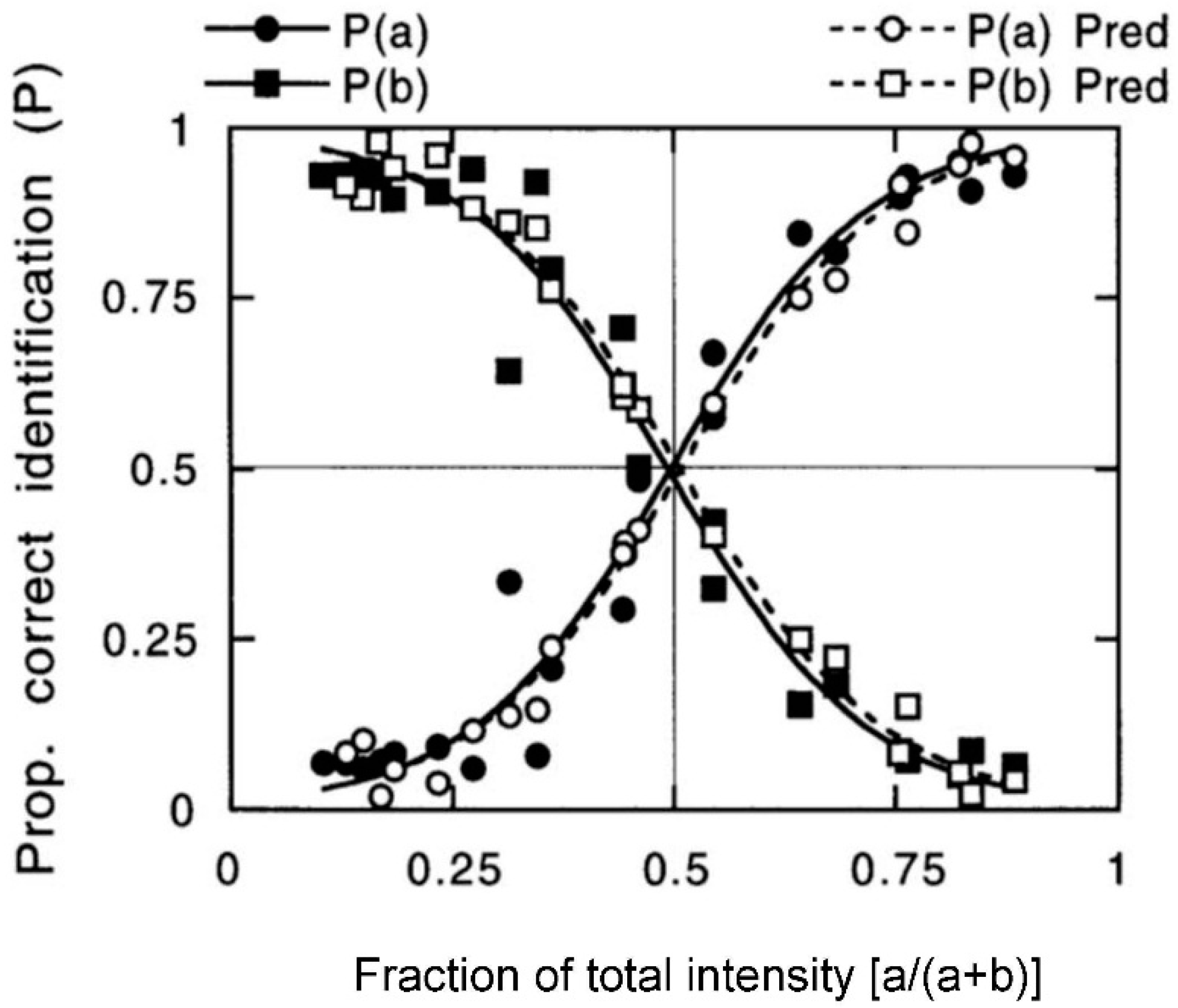
With equally intense components of binary odor mixtures, a unique situation occurs. As shown by Livermore and Laing [13,14], Olsson [15], Olsson and Cain [17] and in the comprehensive review by Ferreira [16], in most cases, both components of the odor mixture could be identified, but with reduced intensity compared to their perception in isolation. Ferreira [16] suggested that both components could be simultaneously recognized, but it is not clear if the individual perceptions occur exactly at the same time. Generally, one component did not dominate the other, a situation that Ferreira [16] referred to as “co-dominance”. In some cases, one component may dominate, but Olsson and Cain [17] suggested that such dominance might not be due to inherent properties of the components but due to unintentionally mismatched intensities. Ferreira [16] concluded that binary mixtures did not form new odor percepts beyond that of the components. Ferreira allowed that some complex mixtures with multiple components could form unique perceptions and referred to the work of Thomas-Danguin et al. [18], who argued for a “configural” perception of odor mixtures. Wilson [19] also supported the idea of a “pattern” percept for mixtures. Saraiva et al. [20] suggested a “combinatorial” effect in binary mixtures on mouse behavior, but this is at odds with many human olfactory studies showing that binary odor mixtures generally do not have unique perceptions.
e.
Probabilities determine component detection. When the intensity of components of binary odor mixtures are not matched, the more intense component tends to suppress or dominate the weaker component. Olsson [15] noted that the dominance is not simply proportional to the relative intensity of the components in the mixture, but is exaggerated. For example, in a study of butanol-pyridine mixtures, if the intensity of one of the components was 1.4 (about the square root of 2) times the other, the probability of detecting the stronger component was about twice the probability of detecting the weaker component. Olsson and Cain [17] provided a simple equation for this relationship: P(a) = RA2/(RA2 + RB2), where P(a) is the probability of detecting component A, RA is the relative intensity of component A in isolation and RB is the relative intensity of component B in isolation. Olsson and Cain [17] summarized their findings as follows: “The probability (P) that a substance A will dominate a mixture of A and B depends on the perceived intensity (R) such that P(a) = RA2/(RA2 + RB2). In other words, the olfactory system seems to accentuate the difference in intensity between two odors when determining a mixture quality”. This concept is discussed later in Section 4, where we present a general model of component interactions.
f.
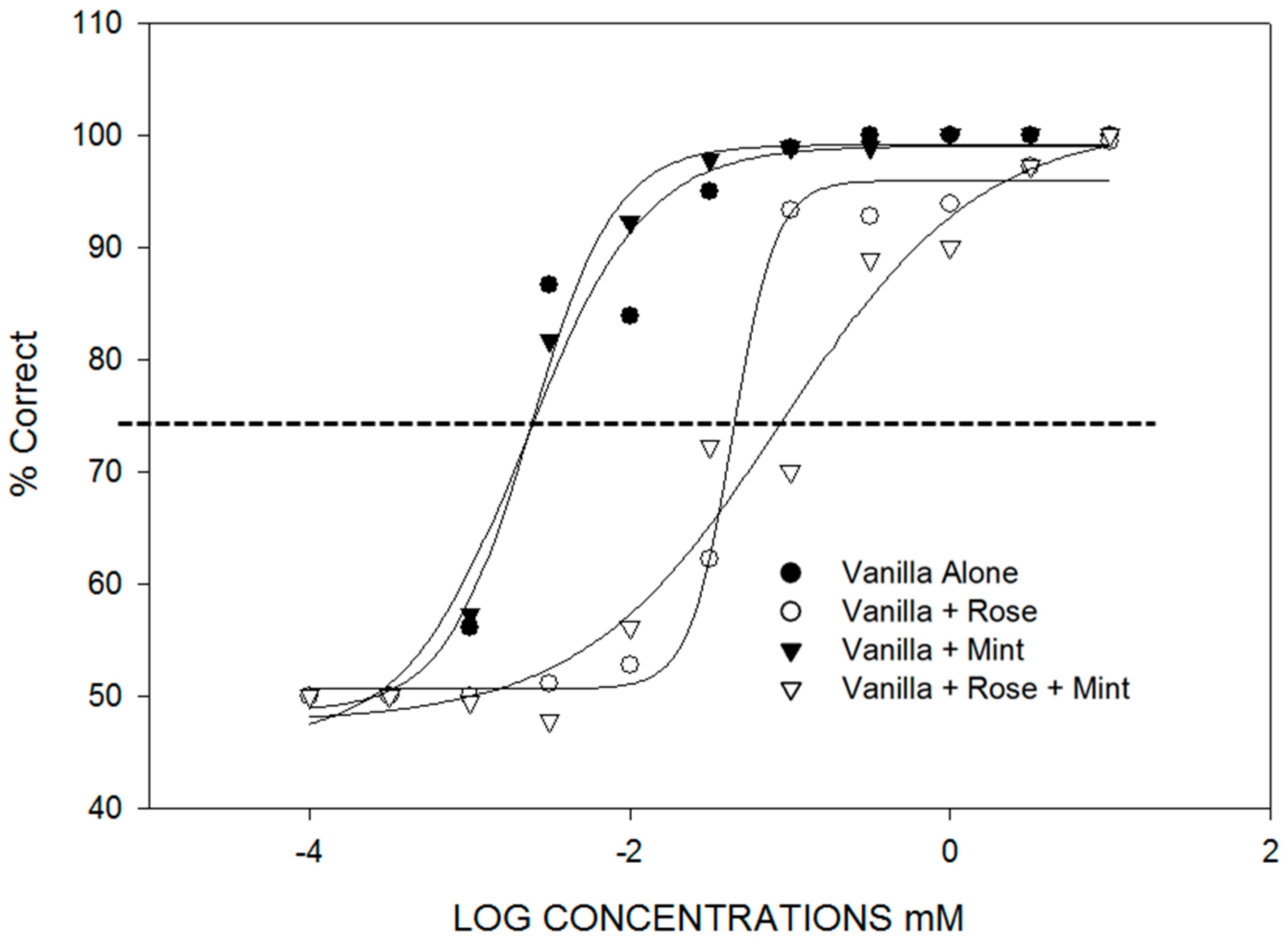
Selective adaptation, background, and genetics affect component identification. There are three situations where identification of components in mixtures reflects the relative intensities of the components in unique ways. The first is the identification of components in mixtures following selective adaptation. This is presented in Section 3. The second case is the identification of a particular odorant in a background of another odorant (Figure 2). In [21], binary and ternary mixtures containing vanillin were found to have vanillin thresholds dependent on the background odorant concentration. For example, vanillin thresholds were raised an order of magnitude in the presence of a background containing phenethyl alcohol. The third case is the identification of odor components in a mixture where genetic differences determine the perception of the components and the mixtures (Figure 3). In [22], individual differences were found in the perception of a mixture of vanillin and beta-ionone that depended on whether the subject had a low or high threshold for beta-ionone, for which a genetic basis is established [23]. “Smellers” and “non-smellers” of beta-ionone differed significantly in their beta-ionone thresholds, but not in their vanillin thresholds. Because of component dominance, “smellers” tended to perceive a mixture of vanillin and beta-ionone to be “violet” and “non-smellers” tended to perceive the same mixture as “vanilla” (Table 2).

3. Selective Adaptation

3.1. Preamble

Sniffing, site, and time course of odor adaptation. Sensory adaptation is a complex phenomenon that is especially difficult to study in olfaction. The act of sniffing produces a variable stimulus intensity and concentrations of odorants at the receptors is unknown. Possible sites of olfactory adaptation include the receptor cell, the olfactory bulb and the olfactory cortex or different cortical areas. The time course of olfactory adaptation is also difficult to assess. The common notion that olfactory adaptation typically occurs over many minutes or hours is probably incorrect. The most rapid process will determine the overall adaptation, wherever its locus. Research of Zufall and Leinders-Zufall [24] places the site of rapid olfactory adaptation within the receptor cell itself. An alternate model [25] would place rapid adaptation in the CNS, but it requires feedback circuits that have not been identified. The most parsimonious model would locate rapid adaptation within the receptor cell. This process may occur with a half-life of a few seconds, though it may not be complete even after many sniffs.

3.2. Selective Adaptation Defined

Selective adaptation occurs when some components of a mixture are preferentially reduced in intensity by prior exposure. In the olfactory system, selective adaptation can be demonstrated by sniffing an odor mixture for a few seconds, followed by sniffing the same mixture with an extra component. The extra component is recognized more readily than the ambient background components.
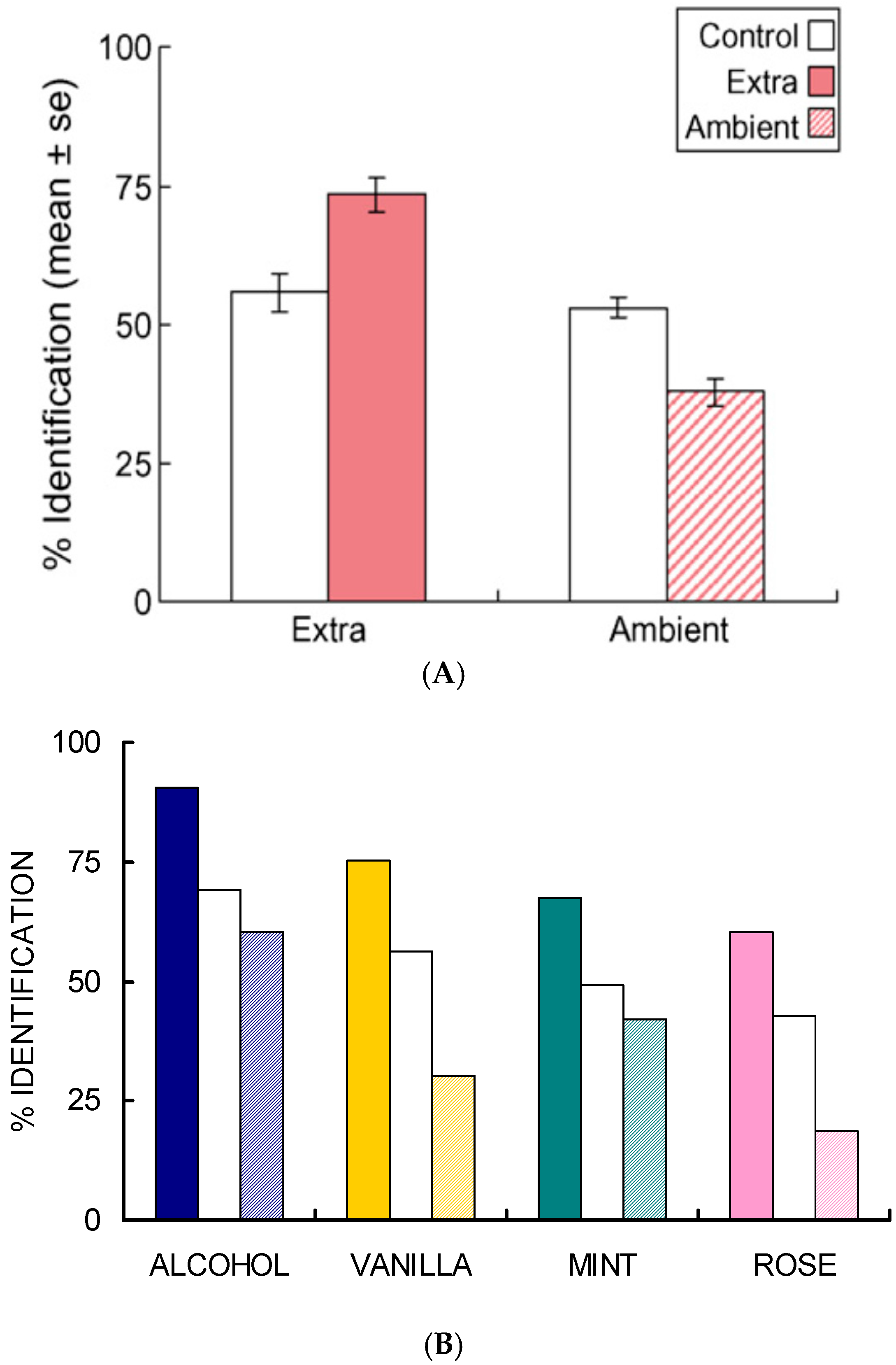
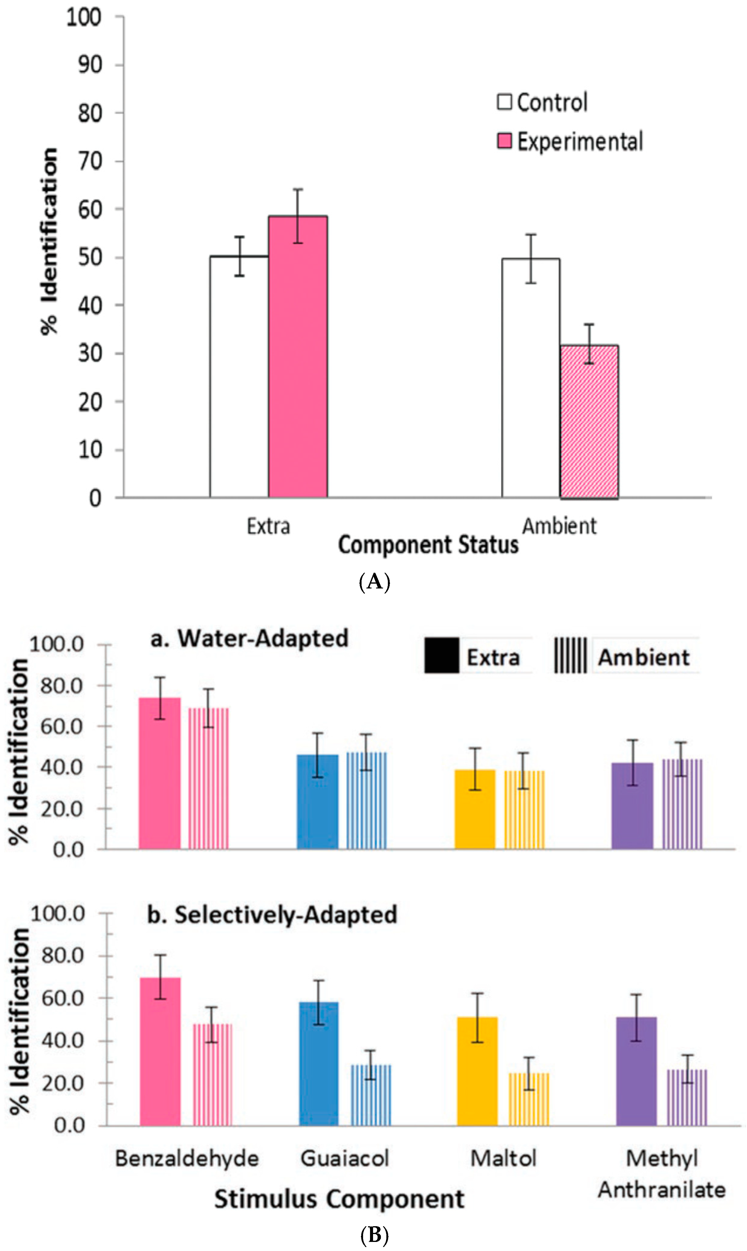
  • Studies of selective adaptation. In our first study [26,27], we used mixtures containing (quality names in parentheses) isopropyl alcohol (alcohol), vanillin (vanilla), l-carvone (mint), and phenethyl alcohol (rose) to determine the effect of selective adaptation (Figure 4). In our second study [28], we used mixtures of benzaldehyde (cherry, almond), guaiacol (smoke), maltol (caramel, cotton candy), and methyl anthranilate (grape) (Figure 5). These two studies gave consistent results for the different four-component mixtures and showed improved ‘extra’ component identification as a result of selective adaptation of ‘ambient’ components.
  • Salient mixture components retain qualities. These different odor sets [26,27,28] suggest that equally salient components retain, to a certain extent, the qualities of the mixture components. In the case of selective adaptation (Figure 4 and Figure 5), odor intensities of the components become unbalanced. Then it is possible to estimate the relative effective concentrations of the ambient and extra components in the mixture. After selective adaptation for about 4 s, identification of the extra component is about twice as likely as identification of the adapted component. The extra component is considered to be dominant. We thus conclude that the process of selective adaptation effectively reduces the apparent concentration of the adapted component to a level about one-half the actual value in the mixture.
  • Adaptation half-life. We would then estimate (assuming first-order kinetics) the half-life (t1/2) for adaptation (in concentration terms) of about 4 s. Using the half-life equation for first-order reactions (k = 0.693/t1/2) we calculate the rate constant for adaptation to be about 0.17 s−1. Of course these are very approximate, but it is important to produce an estimate to compare with known values for adaptation at various levels of the nervous system.
  • Selective taste adaptation. The phenomenon of selective adaptation also occurs in the gustatory system. Our results [29] for taste mixtures of sucrose and sodium chloride showed that extra component identification is improved by selective adaptation to ambient components.

4. Models of Component Interactions in Binary Odor Mixtures

4.1. Preamble

Binary odor mixture component interactions modelled with distinct mathematical formulations yield quite similar symmetric curves. Olsson [15] described a prototypical example (Figure 6). The figure depicts the relation between component-identification proportions and the composition of butanol-pyridine mixtures. The two curves are symmetrical sigmoid functions that cross at the point of equal salience. As the relative intensities of the components diverge, either butanol or pyridine will dominate the perception. The data were fit to logistic functions.

4.2. Probabilities of Component Identification

We developed a model for the identification of components within a binary mixture starting with the general equation of Olsson and Cain [17] which relates the probability of identification of a component P1 as a function of the composition of the binary mixture. We use the same equation of Olsson and Cain, but with different symbols (Equation (1)). P1 is the probability of component 1 identification in the mixture and F1 and F2 are the fractional intensities of the mixture components. We replaced F22 with its equivalent (1 − F1)2 to give Equation (2-1) for P1 and Equation (2-2) for P2 having a single independent variable F1. Note that P1 + P2 = 1 and F1 + F2 = 1.
( Olsson   and   Cain )   P 1 = F 1 2 F 1 2 + F 2 2
( Hettinger   and   Frank )   P 1 = F 1 2 F 1 2 + ( 1 F 1 ) 2
( Hettinger   and   Frank )   P 2 = ( 1 F 1 ) 2 F 1 2 + ( 1 F 1 ) 2
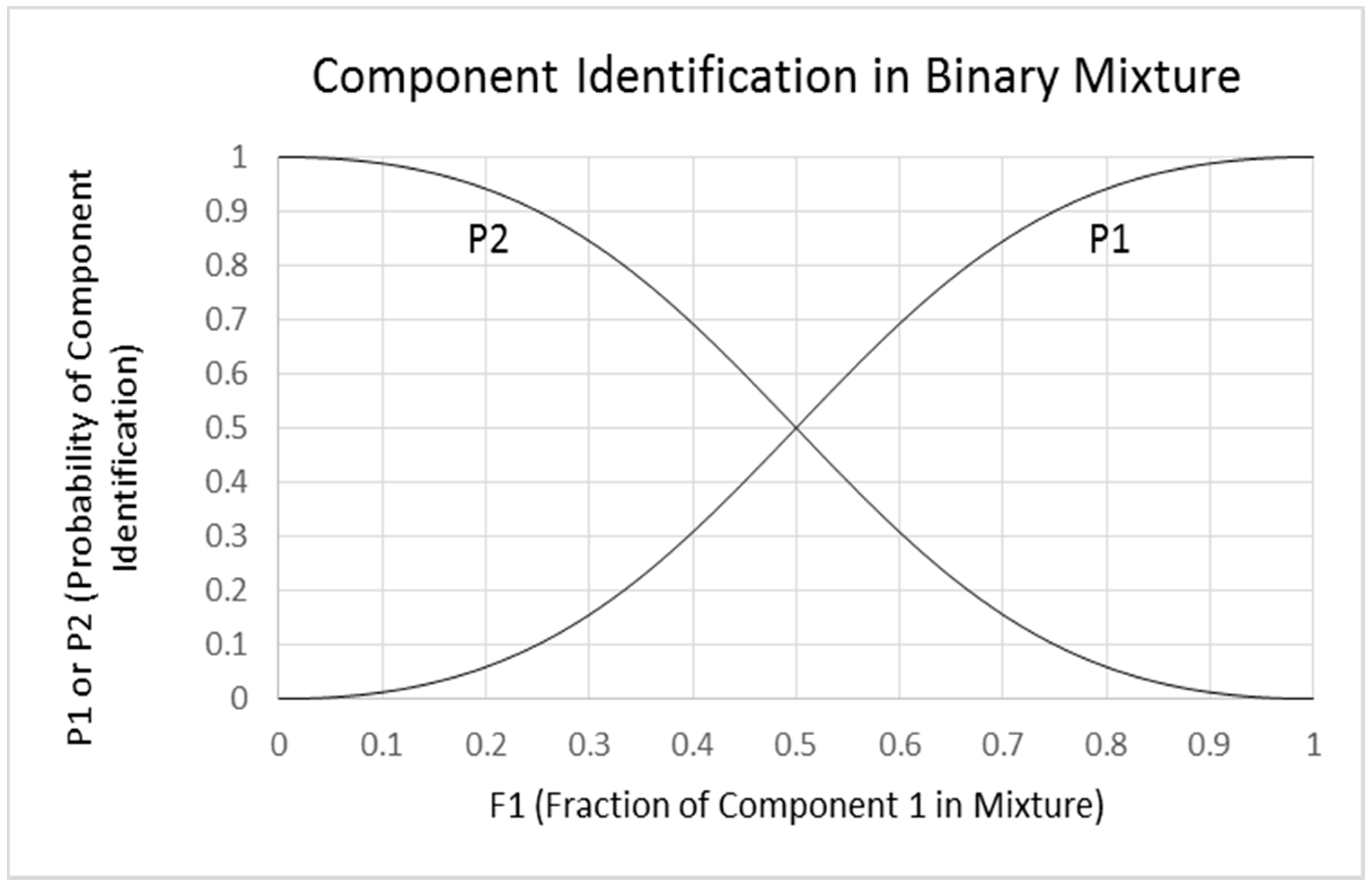
  • Sigmoid/logistic functions. It is notable that a plot of P1 or P2 versus F1 using Equations (2-1) and (2-2) produces sigmoid functions within the defined limits of 0 to 1 for F1. These plots are similar to logistic plots of Ferreira [16], but without logarithmic or exponential operations. The squared intensity terms provide an exaggerated or relatively steep relationship between P1 and F1 in the central region of the plot compared to a linear function. The slope of the equation at the inflection point (0.5, 0.5) is 2, the value of the F1 exponent. It is possible that the exponent could be different for different mixtures, but we consider a value of 2 to be typical for odorants that are orthogonal and have non-overlapping odors. This typical case is shown in Figure 7.
In the original paper by Olsson [15] describing the identification of components of butanol–pyridine mixtures, the curves were fit to unspecified logistic functions. These curves differ slightly from the general equation P1 = F12/(F12 + F22) given by Olsson and Cain [17] because the general equation requires that P1 = 0 when F1 = 0 and P1 = 1 when F1 =1, whereas the logistic functions appear to have a non-zero y intercept due to errors in identification of the pure components. In Olsson’s paper [15], the y intercept is not zero, but about 0.05, corresponding to an error rate of about 5%. In the reanalysis of literature data on odor mixtures, Ferreira [16] fitted the identification probability versus composition curves to logistic functions with calculated slopes and intercepts that have different meanings than those used in our analysis. We adjusted Ferreira’s equations to fit our symbols for the variables P1, P2, and F1 (Equations (3-1) and (3-2)). The two equations are related by symmetry and differ only in the sign of the exponent.
( Ferreira )   P 1 = 1 1 + 10 ( F 1 b ) / a
( Ferreira )   P 2 = 1 1 + 10 ( F 1 b ) / a
Ferreira’s slope parameter (a) in the exponent of the exponential function is related to the shallowness of the function, not the typical value of dy/dx at the inflection point used in our model. Ferreira’s intercept parameter (b) corresponds to the point of equal component intensity and differs conceptually from our intercept, the relative identification error. Some of the odor pairs described by Ferreira had rather shallow functions and had y intercepts (equal to b in our definition in Figure 8) of about 0.1, implying substantial misidentification of the pure components.
In some of Ferreira’s plots, it is notable that P1 and P2 are not equal to 1 even when F1 and F2 values are equal to 1. This is especially true when the slope parameter (a) is large (about 0.53), where P1 is only about 0.9 when F1 = 1, which indicates that the components are not perfectly recognized even when alone. This raises the important issue of orthogonality, or whether the components are distinct enough to be separately recognized. We made the presumption that, in order for the dominance rules to be established with conviction, the odor components of each pair should be distinct. If components have similar odor quality such as occurs in isomeric esters [30] or periodic table analogs [31], they would not exhibit strong dominance because they would be hard to distinguish.
b.
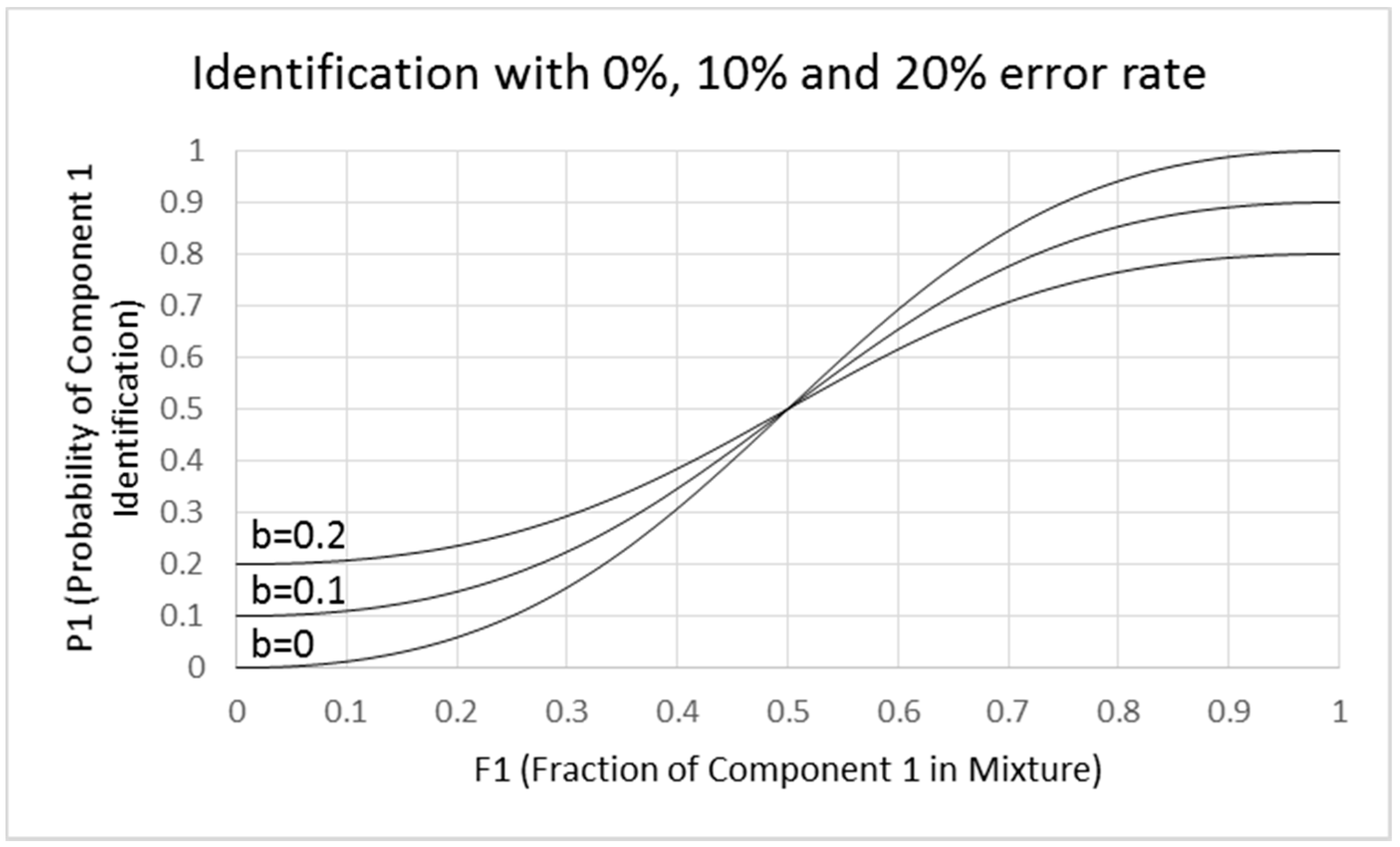
Misidentifications. Though Ferreira did not consider identification errors in explaining the logistic fits, it is likely that the flat functions are due to misidentifications. We show in Figure 8 examples of how this could occur. We made pragmatic adjustments of Equations (2-1) and (2-2) to develop Equations (4-1) and (4-2), which show increasing flattening of the sigmoid function with increasing error rate defined by intercept b. The slope at the inflection point is 2(1 − 2b). When b = 0, the curve is identical to that shown in Figure 8 with a slope of 2. When b = 0.1, the slope is reduced to 1.6, and when b = 0.2, the slope is 1.2. This result suggests that the flattening of the function can be due to identification errors rather than a change in the exponent of the fractional component intensity. It also indicates that analysis of mixtures with extensively overlapping odor qualities would be difficult. Analysis of mixtures works best when odors are orthogonal and non-overlapping. An exponent of 2 for the fractional component intensities in binary mixtures may be a general property for orthogonal odorants.
( Hettinger   and   Frank )   P 1 = ( 1 b ) F 1 2 + b ( 1 F 1 ) 2 F 1 2 + ( 1 F 1 ) 2
( Hettinger   and   Frank )   P 2 = ( 1 b ) ( 1 F 1 ) 2 + bF 1 2 F 1 2 + ( 1 F 1 ) 2
c.
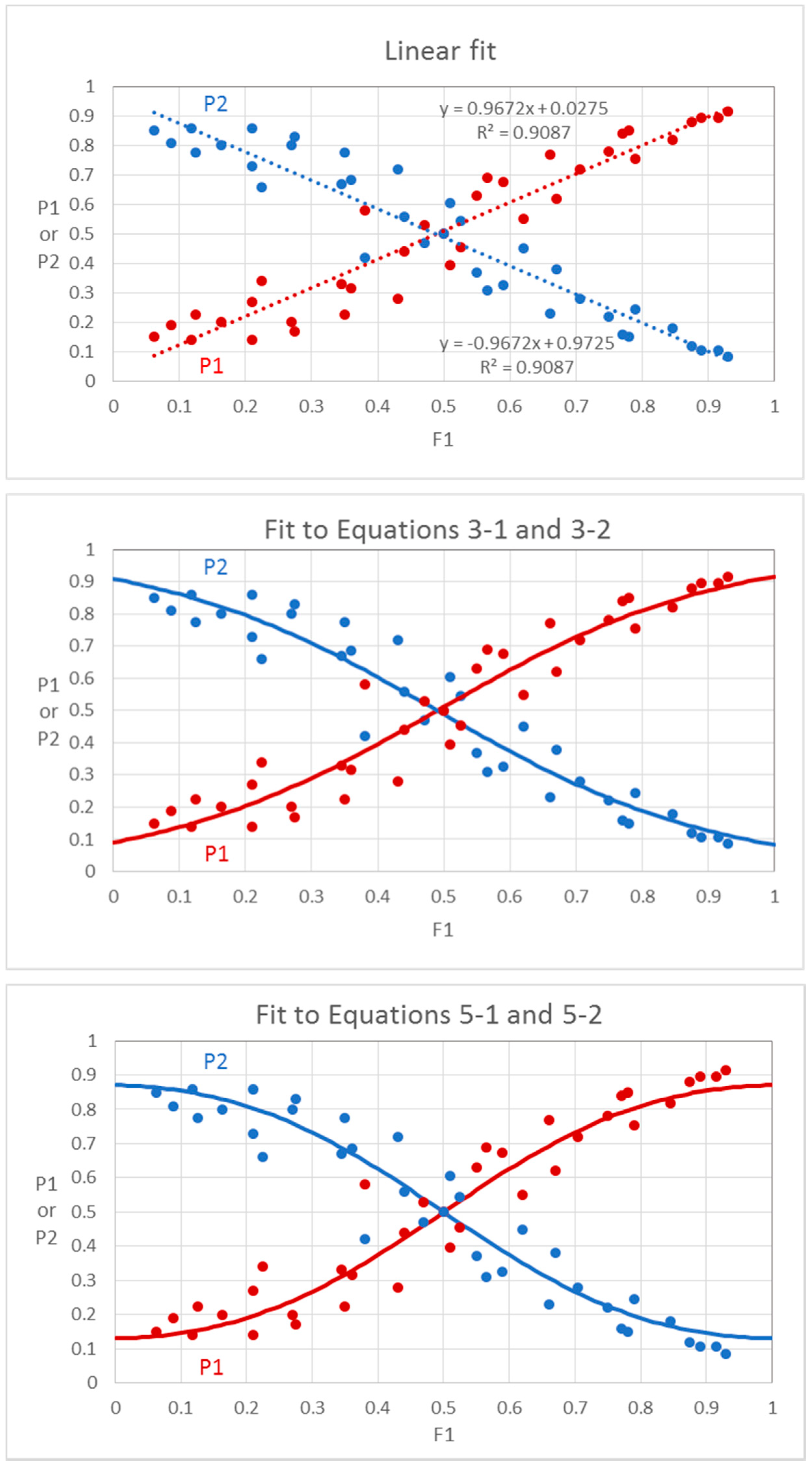
Exponent effects. Finally, we also consider equations where the exponent of F1 may not be 2 but could be any positive value = n (Equations (5-1) and (5-2)). The value of n is analogous to the Hill coefficient in enzyme kinetics where it is related to cooperativity among subunits. The value of n has no clear meaning for dominance in odor mixtures, but it may be speculated that values of n greater than 1 represent convergent neural activity in the CNS. Because Equations (5-1) and (5-2) cannot be linearized, the b and n parameters are determined by successive approximation and minimizing the sum of squared deviations of P1 from the fitted line. We provide an example in Supplementary Material of how data can be fit to Equations (5-1) and (5-2) in an Excel program.
( Hettinger   and   Frank )   P 1 = ( 1 b ) F 1 n + b ( 1 F 1 ) n F 1 n + ( 1 F 1 ) n
( Hettinger   and   Frank )   P 2 = ( 1 b ) ( 1 F 1 ) n + bF 1 n F 1 n + ( 1 F 1 ) n
We extracted odor mixture data from Figure 2a of Ferreira [16], which describes odor dominance in eugenol/propionic acid mixtures. We then fit the P versus F values to Equations (3-1) and (3-2) (Ferreira) and Equations (5-1) and (5-2) (Hettinger and Frank). The optimum fits to either pair of equations have similar sum of squared deviations (0.2035 for Equations (3-1) and (3-2) and 0.2034 for Equations (5-1) and (5-2) and both are better than the value of 0.2250 for a straight line fit (Figure 9). The straight line fit has an R2 value of 0.909, while the fits to Equations (3-1), (3-2), (5-1), and (5-2) all have R2 values of about 0.917, which is only approximate because R2 is rigorously defined only for linear fits. The sigmoid shape of the data is only marginally evident because of the high scatter of the points. The lines fitted to Equations (3-1) and (3-2) have a slope value a = 0.49 and a co-dominance point of b = 0.49. These values differ slightly from those reported by Ferreira because he used linearized logistic plots that give different weights to the data points. Ferreira’s plot crosses the y-axis at 0.083 (fractional identification error). The fit to Equations (5-1) and (5-2) has an optimum b intercept value of 0.13 (error) and an optimum n value of 1.75 (exponent). Ferreira’s equation does not provide an exponent of F1, as the slope value is a factor of F1, not an exponent of F1. Although Ferreira’s model and our model fit the experimental data equally well, we believe that Equations (5-1) and (5-2) are improvements because they provide an explicit interpretation of the parameters b and n. It is peculiar that much of the literature on mixtures does not provide a direct estimate of the identification error b, when it would be easy to do by determining the misidentification rate of the pure components. Possibly the pure components were not used because the logistic fits could not deal with F1 values of 0 or 1. This is not a problem in our model because it does not use logistic functions. Our model applies only to cases where the two plots are symmetrical and where P1 and P2 values are equal or nearly equal to 0.5 when F1 equals 0.5, which indicates that the components are equal in their effects on perception of the binary mixture. Ferreira described cases of binary mixtures where the two plots are asymmetrical and cross at values of F1 different from 0.5, which implies that one component dominates the perception even when both components are equally intense. We made no attempt to model this situation, which would require an additional parameter to fit the data. The existence of asymmetry in binary odor mixture perception is currently not understood. A detailed analysis is given in Supplementary Material, which provides interactive Excel spreadsheets for adjusting the parameters of Equations (3-1), (3-2), (5-1), and (5-2) to optimize fitting of the lines to the data.
In his analysis of binary odor mixtures, Ferreira [16] concluded that in a typical or average case, the ratio of identification probabilities is about 2 when the component intensities in isolation are in the ratio of 59/41 or about 1.4 or the square root of 2. This fits with the general equation of Olsson and Cain [17]. Ferreira also considered that one component would be dominant when the ratio of identification probabilities is 2 or more. Thus, one component will dominate the other by at least a factor of 2 if its intensity is 59% or more of the summed intensities of the components.
d.
One or two sniffs can reduce ambient component intensity by a factor of 1.4. In our studies [26,27,28] on selective adaptation (Figure 4 and Figure 5), we observed that, for two different datasets each involving four components in various mixture combinations, extra components were on average identified twice as often as ambient components which had been partially adapted over a few seconds. This suggests that the intensity of the ambient components had been reduced by a factor of about 1.4 during one or two sniffs. Of the eight different odorants used in the two studies, the individual components were identified with an accuracy of about 90%, except for methyl anthranilate, which was correctly identified only about 60% of the time. It is difficult to generate mixtures of four or more components where each component has an odor completely distinct from the others.
e.
Detecting odor mixture interactions. Models of odor interactions in mixtures are dependent on how odor intensity is measured and how component intensities are matched. In the sensory psychology literature, perceived odor intensity is considered to be a power function of odorant concentration (Stevens’ power law). We assumed a typical value for the concentration exponent to be about 0.5 according to the equation I = kC0.5, where I is the perceived intensity, C is the odorant concentration and k is a constant. When comparing different odorants with different and unknown values of k, odor intensities are typically determined by magnitude estimation, and matched by direct comparison of perceived odor intensities or by cross-modality matching. This is a difficult procedure that involves subjective judgments that are prone to bias and other errors. As noted in Section 2, in an attempt to produce a more objective measure of odor intensity, flavor, and fragrance studies use the concept of odor activity value (OAV), which is the ratio of odorant concentration to its threshold value [4]. This method has been criticized because in comparing different odorants in mixtures, OAVs were not considered to be additive in the same way as odor intensities. However, as shown in Section 2 for a binary mixture, we were able to eliminate k from the paired power law equations and generate a new equation for the relationship between perceived intensity and OAV for mixture components: I 1 / I 2 = ( OAV 1 / OAV 2 ). This means that the ratio of odor intensities is (approximately) equal to the square root of the ratio of their respective OAV values.
Thus, if one considers the typical case [16] for a binary mixture presented above where P1/P2 = 2 when I1/I2 = 1.4, we can conclude that P1/P2 = 2 when (OAV1/OAV2) is (approximately) 2. More generally, the ratio of the component identifications is approximately equal to the ratio of the component OAVs. This would be true for component dominance in binary mixtures where the intensities have been intentionally mismatched or if components become mismatched by selective adaptation. In the case of selective adaptation, we conclude that selective adaptation for a few seconds reduces the identification ratio and the OAV of the ambient component by about 50%.
f.
Analytic odor perception. Our treatment is explicitly analytical and does not consider odor mixtures to have synthetic properties. The treatments of Olsson [15] and Ferreira [16] are also analytical, while there are many researchers who consider olfaction to be synthetic or combinatorial like color vision. Thomas-Danguin et al. [18] and Wilson [19] have argued for configural or synthetic processing of odor mixtures. We do not disagree with their approach, but we think there are strong arguments for treating odor mixtures as resolvable into components. Combinatorial arguments based on receptor activation [6] for pure compounds and mixtures use the relatively broad tuning of receptors to imply that odor perception is essentially synthetic. However, activation of broadly tuned receptors could be neutralized or suppressed by activation of other more efficacious and selective receptors. In this way, the combinatorial process is more a process of subtraction than addition, with the more intense components dominating the perception.
g.
A unique or synthesized perception? A combinatorial process was also invoked for binary odor mixtures in mice [20]. Though not explicitly stated, the combinatorial model involves a unique or synthetic perception for binary mixtures. Olsson [15], Olsson and Cain [17], and Ferreira [16] have discussed typical situations where binary odor mixtures are perceived as two distinct components, and we have argued that both components are often perceived in binary mixtures if the components are present at equal intensities. When the components are not balanced in intensity, generally one component will dominate the perception. Even when perceptual intensities are matched and both components are recognized, it is likely that the individual components are identified in a probabilistic manner, so both components are not recognized exactly at the same time. If we were to propose that both components could be recognized simultaneously, this would amount to a synthetic composition, in which neither component could actually be recognized, negating the original premise. As in the case of color vision, red and green cannot be simultaneously recognized.
We also observed in animal [32,33] as well as human [29] taste experiments that individual components can be recognized in mixtures. There is less room for a combinatorial argument for taste because the receptors are fewer, the perceptions are distinct and the chemical structures are very different for the different taste qualities.
The mechanism of component dominance and mixture suppression most likely occurs in the olfactory bulb, where extensive inhibitory circuits serve to suppress activity between glomeruli [10,11]. A recent hypothetical model invokes receptor antagonism for mixture suppression [7]. However, there are very few examples of receptor antagonism that have been demonstrated experimentally [8,9]. A key factor in support of a neural basis for olfactory antagonism in mixtures is that antagonism is almost universal among odorants and is especially evident when components are distinctly different. The site of rapid selective adaptation most likely occurs in the receptor cell itself, which has feedback pathways for altering second messenger levels on the scale of a few seconds [24].

5. Summary and Conclusions

This commentary focuses on selective adaptation and mixture suppression of odors in humans. The chemosensory world comprises individual odor and taste chemicals often in complex mixtures. The natural environment of olfaction is often sparse, with a few or no odorants present at any given time. The olfactory system with its many receptors is exquisitely sensitive and can detect and recognize odorants at extremely low concentrations. Often a single odorant can define the perception of an odor object. At near threshold levels, odorants activate only a few of the most sensitive receptors. At higher concentrations, other receptors are activated, but they can be suppressed by increased activation of the most sensitive receptors through inhibitory circuits in the olfactory bulb, which allows the perceptual quality of odorants to remain constant. The taste system has fewer receptors that detect stimuli at higher concentrations that are appropriate for nutrition. Mixtures of chemosensory stimuli, whether taste or smell, are perceived in a temporally fluctuating manner in which individual components can nevertheless be recognized. Mathematical models developed for binary mixture perceptions appropriately predicted the 0 to 1 range of probabilities and measured subject error rates. When components are not balanced in intensity, it is generally the most salient component that dominates perception. In the process of sniffing or tasting, stimuli are partially adapted in a few seconds, allowing new and unadapted stimuli to be perceived. In this way, chemical senses employ subtraction by mixture suppression and selective adaptation to resolve components combined in complex mixtures into their component parts.

Supplementary Materials

Supplementary materials can be found online at https://www.mdpi.com/2227-9040/6/4/44/s1.

Acknowledgments

We acknowledge funding by the UCONN Medical Clinical Research Center, UCONN Research Foundation, UCONN Dental Clinical Research Center; and the work of our students: Ashley N. Phares and Lauren K. Dulieu.

Conflicts of Interest

The authors declare no conflict of interest.

References

  1. Frank, M.E. Chapter 10, Chemoreception and Perception. In Fundamentals of Oral Histology and Physiology; Hand, A.R., Frank, M.E., Eds.; Wiley and Sons: Hoboken, NJ, USA, 2014; pp. 191–217. [Google Scholar]
  2. Dieris, M.; Ahuja, G.; Krishna, V.; Korsching, S.I. A single identified glomerulus in the zebrafish olfactory bulb carries the high-affinity response to death-associated odor cadaverine. Sci Rep. 2017, 7, 40892. [Google Scholar] [CrossRef] [PubMed] [Green Version]
  3. Bushdid, C.; Magnasco, M.O.; Vosshall, L.B.; Keller, A. Humans can discriminate more than 1 trillion olfactory stimuli. Science 2014, 343, 1370–1372. [Google Scholar] [CrossRef] [PubMed]
  4. Grosch, W. Determination of potent odourants in foods by aroma extract dilution analysis (AEDA) and calculation of odour activity values (OAVs). Flavour Fragr. J. 1994, 9, 147–158. [Google Scholar] [CrossRef]
  5. Cometto-Muñiz, J.E.; Abraham, M.H. Dose-Response Functions for the Olfactory, Nasal Trigeminal, and Ocular Trigeminal Detectability of Airborne Chemicals by Humans. Chem. Senses 2016, 41, 3–14. [Google Scholar] [CrossRef] [PubMed]
  6. Malnic, B.; Hirono, J.; Sato, T.; Buck, L.B. Combinatorial receptor codes for odors. Cell 1999, 96, 713–723. [Google Scholar] [CrossRef]
  7. Reddy, G.; Zak, J.D.; Vergassola, M.; Murthy, V.N. Antagonism in olfactory receptor neurons and its implications for the perception of odor mixtures. eLife 2018, 7, e34958. [Google Scholar] [CrossRef] [PubMed] [Green Version]
  8. Oka, Y.; Nakamura, A.; Watanabe, H.; Touhara, K. An odorant derivative as an antagonist for an olfactory receptor. Chem. Senses 2004, 29, 815–822. [Google Scholar] [CrossRef] [PubMed]
  9. Brodin, M.; Laska, M.; Olsson, M.J. Odor interaction between Bourgeonal and its antagonist undecanal. Chem. Senses 2009, 34, 625–630. [Google Scholar] [CrossRef] [PubMed]
  10. Yu, Y.; Migliore, M.; Hines, M.L.; Shepherd, G.M. Sparse coding and lateral inhibition arising from balanced and unbalanced dendrodendritic excitation and inhibition. J. Neurosci. 2014, 34, 13701–13713. [Google Scholar] [CrossRef] [PubMed]
  11. Storace, D.A.; Cohen, L.B. Measuring the olfactory bulb input-output transformation reveals a contribution to the perception of odorant concentration invariance. Nat. Commun. 2017, 8, 81. [Google Scholar] [CrossRef] [PubMed]
  12. Laing, D.G. Natural sniffing gives optimum odour perception for humans. Perception 1983, 12, 99–117. [Google Scholar] [CrossRef] [PubMed]
  13. Livermore, A.; Laing, D.G. Influence of training and experience on the perception of multicomponent odor mixtures. J. Exp. Psychol. Hum. Percept. Perform. 1996, 65, 267–277. [Google Scholar] [CrossRef]
  14. Livermore, A.; Laing, D.G. The influence of odor type on the discrimination and identification of odorants in multicomponent odor mixtures. Physiol. Behav. 1998, 65, 311–320. [Google Scholar] [CrossRef]
  15. Olsson, M.J. An integrated model of intensity and quality of odor mixtures. Ann. N. Y. Acad. Sci. 1998, 30, 837–840. [Google Scholar] [CrossRef]
  16. Ferreira, V. Revisiting psychophysical work on the quantitative and qualitative odour properties of simple odour mixtures: A flavour chemistry view. Part 2, qualitative aspects. A review. Flavour Fragr. J. 2012, 27, 201–215. [Google Scholar] [CrossRef]
  17. Olsson, M.J.; Cain, W.S. Psychometrics of odor quality discrimination: Method for threshold determination. Chem. Senses 2000, 25, 493–499. [Google Scholar] [CrossRef] [PubMed]
  18. Thomas-Danguin, T.; Sinding, C.; Romagny, S.; El Mountassir, F.; Atanasova, B.; Le Berre, E.; Le Bon, A.M.; Coureaud, G. The perception of odor objects in everyday life: A review on the processing of odor mixtures. Front. Psychol. 2014, 5, 504. [Google Scholar] [CrossRef] [PubMed]
  19. Wilson, D.A. Pattern separation and completion in olfaction. Ann. N. Y. Acad. Sci. 2009, 1170, 306–312. [Google Scholar] [CrossRef] [PubMed]
  20. Saraiva, L.R.; Kondoh, K.; Ye, X.; Yoon, K.H.; Hernandez, M.; Buck, L.B. Combinatorial effects of odorants on mouse behavior. Proc. Natl. Acad. Sci. USA 2016, 113, E3300–E3306. [Google Scholar] [CrossRef] [PubMed]
  21. Phares, A.N.; Frank, M.E.; Hettinger, T.P. Effects of background stimuli on odor detection thresholds. In Proceedings of the AChemS Meeting, St. Pete Beach, FL, USA, 13–17 April 2011; UCONN Health, Dental Medicine: Farmington, CT, USA, 2011. [Google Scholar]
  22. Dulieu, L.K.; Frank, M.E.; Hettinger, T.P. Discovering Qualities of Single-Stimuli Mixtures Having Double Odors; UCONN Health, Dental Medicine: Farmington, CT, USA, 2015. [Google Scholar]
  23. McRae, J.F.; Jaeger, S.R.; Bava, C.M.; Beresford, M.K.; Hunter, D.; Jia, Y.; Chheang, S.L.; Jin, D.; Peng, M.; Gamble, J.C.; et al. Identification of regions associated with variation in sensitivity to food-related odors in the human genome. Curr. Biol. 2013, 23, 1596–1600. [Google Scholar] [CrossRef] [PubMed]
  24. Zufall, F.; Leinders-Zufall, T. The cellular and molecular basis of odor adaptation. Chem. Senses 2000, 25, 473–481. [Google Scholar] [CrossRef] [PubMed]
  25. Li, Z.; Hertz, J. Odour recognition and segmentation by a model olfactory bulb and cortex. Netw. Comput. Syst. 2000, 11, 83–102. [Google Scholar] [CrossRef] [Green Version]
  26. Goyert, H.F.; Frank, M.E.; Gent, J.F.; Hettinger, T.P. Characteristic component odors emerge from mixtures after selective adaptation. Brain Res. Bull. 2007, 72, 1–9. [Google Scholar] [CrossRef] [PubMed] [Green Version]
  27. Frank, M.E.; Goyert, H.F.; Hettinger, T.P. Time and intensity factors in identification of components of odor mixtures. Chem. Senses 2010, 35, 777–787. [Google Scholar] [CrossRef] [PubMed]
  28. Frank, M.E.; Fletcher, D.B.; Hettinger, T.P. Recognition of the Component Odors in Mixtures. Chem. Senses 2017, 42, 537–546. [Google Scholar] [CrossRef] [PubMed] [Green Version]
  29. Frank, M.E.; Goyert, H.F.; Formaker, B.K.; Hettinger, T.P. Effects of selective adaptation on coding sugar and salt tastes in mixtures. Chem. Senses 2012, 37, 701–770. [Google Scholar] [CrossRef] [PubMed]
  30. Poivet, E.; Tahirova, N.; Peterlin, Z.; Xu, L.; Zou, D.J.; Acree, T.; Firestein, S. Functional odor classification through a medicinal chemistry approach. Sci. Adv. 2018, 4, eaao6086. [Google Scholar] [CrossRef] [PubMed]
  31. Doszczak, L.; Kraft, P.; Weber, H.P.; Bertermann, R.; Triller, A.; Hatt, H.; Tacke, R. Prediction of perception: Probing the hOR17-4 olfactory receptor model with silicon analogues of bourgeonal and lilial. Angew. Chem. Int. Ed. Engl. 2007, 46, 3367–3371. [Google Scholar] [CrossRef] [PubMed]
  32. Frank, M.E.; Formaker, B.K.; Hettinger, T.P. Taste responses to mixtures: Analytic processing of quality. Behav. Neurosci. 2003, 117, 228–235. [Google Scholar] [CrossRef] [PubMed]
  33. Frank, M.E.; Lundy, R.F., Jr.; Contreras, R.J. Cracking taste codes by tapping into sensory neuron impulse traffic. Prog. Neurobiol. 2008, 86, 245–263. [Google Scholar] [CrossRef] [PubMed] [Green Version]
Figure 1. Structures of odor objects captured by one compound. The 20 chemicals occur in nature and have different, distinct odors that represent a wide range of chemical structure and odor variety. In contrast to color vision (based on three pigments with sensitivities peaking at blue, green, or red regions of visible electromagnetic spectra), there are tens of taste receptors and hundreds of odor receptors tuned to water-soluble and vaporous chemicals, respectively. The 20 times as many olfactory-neuron than taste-cell receptor variants match numerical differences in distinct odors and tastes perceived. From [1] with permission from Wiley.
Chemosensors 06 00044 g001
Figure 2. Odor mixture interactions: vanilla plus background. Near-threshold background stimuli affected vanilla odor detection. Background odors were at a constant 0.032 mM concentration. With the exception of l-menthol, vanilla odor detection threshold in mixtures increased by 1 log unit (vanillin + phenethyl-alcohol, p = 0.0001; vanillin + phenethyl − alcohol + l-menthol, p = 0.0001). Vanilla-odor detection threshold possibly increased in presence of background containing rose odor because of olfactory-bulb glomerular competitive mutual suppression. The mint background did not affect vanilla detection. Menthol also elicits a cool sensation. Whether stimuli with trigeminal components behave differently from pure odors in mixtures has not been tested. From [2].
Chemosensors 06 00044 g002
Figure 3. Odor mixture interactions: genetics. Vanillin thresholds do not differ for ‘smellers’ and non-smellers of β-ionone. β-ionone thresholds for ‘non-smellers’ are all higher than thresholds for ‘smellers’. From [22]. The β-ionone smeller detects a ‘violet-flower’ odor; whereas, the non-smeller detects ‘woody’. Results are generally consistent with McRae et al. [23], who found ‘non-smellers’ of β-ionone to have a threshold more than an order of magnitude higher than ‘smellers’.
Chemosensors 06 00044 g003
Figure 4. Selective adaptation of alcohol, vanilla, mint and rose odors in 2, 3, and 4 component mixtures. (A) Correct identification increased for newly introduced extra stimuli, p < 0.0001, but decreased for continuing ambient stimuli, compared to controls, p < 0.001. (B) Extra component identification is greater (solid color bars) and ambient component is poorer (striped color bars) than controls (white bars). From [26] with permission from Elsevier.
Chemosensors 06 00044 g004
Figure 5. Selective adaptation of cherry, smoke, caramel and grape odors in 2, 3, and 4 component mixtures replicates the results shown in Figure 4 for alcohol, vanilla, mint and rose in spite of benzaldehyde cherry-odor dominance. From [28] with permission of Oxford University Press. (A) Results for a second foursome of odors: cherry, smoke, caramel, and grape replicate first shown in Figure 4. Experimental: selectively adapted (rose-colored bars). Control: water-adapted (white bars). (B) Although benzaldehyde dominates water-adapted mixtures (a); extra components dominate selectively-adapted mixtures (b).
Chemosensors 06 00044 g005
Figure 6. Binary odor mixture identification: Olsson model [15]. The plots show identification proportions for butanol/pyridine as a function of composition (fractional intensity). Fit of the Olsson model (open symbols) to empirical data (filled symbols) is good. The r = 0.98 for prediction of proportional quality. Mixed ‘odors of equal intensity’ have equally prominent components. From [15] with permission from Wiley.
Chemosensors 06 00044 g006
Figure 7. Binary mixture odor identification: Hettinger and Frank model. P1 shows a plot of the probability of identification (P1) of component 1 as a function of the relative intensity (F1) of component 1. P2 shows the corresponding plot for the identification of component 2. The plot is for the equation P1 = F12/(F12 + (1 − F1)2) and is based on the equation of Olsson and Cain [17] where P1 = F12/(F12 + F22). The two plots are symmetric and sigmoid, with the points at 0.5 corresponding to matched intensities of the two components. P1 and P2 are the probabilities of identification of components 1 and 2, respectively, where P1 + P2 = 1. F1 and F2 are the fractional intensities of the respective unmixed components, where F1 + F2 = 1. The steepness of the functions is determined by the F1 and F2 exponents, which in the general model equals 2. The slope (dy/dx) at the inflection point is equal to 2 for the P1 function and −2 for the P2 function.
Chemosensors 06 00044 g007
Figure 8. Binary mixture odor identification error: Hettinger and Frank model. Model of component identification showing effect of identification errors show three binary-odor identification error-rates for mixture components. Errors are reflected in the existence of an intercept b for the P1 function when F1 = 0. Three plots are given: (1) b = 0 where no identification errors occur, (2) b = 0.1 where the error rate is 10% and (3) b = 0.2 where the error rate is 20%. The plots are for the equation P1 = [(1 − b)F12 + b(1 − F1)2]/[F12 + (1 − F1)2] which shows increasing flattening of the function with increasing error rate. The slope at the inflection point is 2 × (1 − 2b). When b = 0, the curve is identical to that shown for P1 in Figure 7. The slope and intercept have different meanings from those of Ferreira [16].
Chemosensors 06 00044 g008
Figure 9. Probability of identification of components in eugenol-propionic acid mixtures. Data extracted from Figure 2a of Ferreira [16]. P1 is the probability of identification of eugenol (red points), P2 is the probability of identification of propionic acid (blue points), and F1 is the fractional intensity of eugenol in the mixture. The top graph shows fit to straight line, the middle graph shows fit to Ferreira model, and the bottom graph shows fit to Hettinger and Frank model. The fits of both models are equally good, and better than the linear fit. Details of fitting of models can be found in Supplementary Material. Extracted from [16] with permission from Wiley.
Chemosensors 06 00044 g009
Table 1. Chemosensory receptors with distinct chemistries.
Number of Variants
ReceptorsReceptor CellsSensory Neurons
Total Olfactory Receptors (OR)390390390
Total Taste Receptors (TR)3455
Taste Receptor (TR)T1R dimer222
T2R3011
ENaC111
PKD dimer111
Olfactory and Taste424395
In contrast to color vision (based on three pigments with sensitivities peaking at blue, green, or red regions of visible electromagnetic spectra), there are tens of taste receptors and hundreds of odor receptors tuned to water-soluble and vaporous chemicals, respectively. The 20 times as many olfactory-neurons than taste-cell receptor variants match numerical differences in distinct odors and tastes perceived. From [1] with permission from Wiley.
Table 2. Responses of β-ionone (‘violet odor’) smellers and β-ionone non-smellers to mixtures with 10 ppm vanillin (‘vanilla odor’).
β-Ionone ppb‘Smellers’ (n = 12)‘Non-Smellers’ (n = 4)
(1) 10 ppbIdentifications
Violet only10
Vanilla only124
Both30
(2) 100 ppb
Violet only80
Vanilla only74
Both80
(3) 1000 ppb
Violet only123
Vanilla only01
Both44
Choice of ‘vanilla’, ‘violet’, or ‘both’ on at least one of the three trials counted as an identification. (1). ‘Violet’ was rarely identified in 10 ppb β-ionone by ‘smellers’ or ‘non-smellers’; (2). While ‘smellers’ identified ‘violet’ and ‘both’ odors, non-smellers failed to identify either in 100 ppb β-ionone. Chi square = 6.83, df = 2, p = 0.033; (3). ‘Violet’ and ‘both’ odors prevailed in all subjects at 1000 ppb β-Ionone, a concentration in which ‘non-smellers’ detect a woody odor. From [22].

