Rapid Geographical Origin Discrimination of Tremella fusiform Based on Temporal Response Features of Electronic Nose

Abstract

Rapid geographical origin discrimination of Tremella fuciformis is important for quality control and authenticity assessment; however, conventional analytical methods are often time-consuming and require complex sample preparation. In this study, a rapid discrimination approach was established by integrating electronic nose (E-nose) response fingerprints with machine learning. To capture temporal variation in the E-nose signals, fingerprint features were extracted from three response windows: the selected overall response window (0–69 s), the early response window (0–29 s), and the relatively stable response window (56–65 s). Random forest, partial least squares discriminant analysis (PLS-DA), Gaussian naive Bayes, nearest centroid, and decision tree were then constructed and evaluated. Classification performance varied among the temporal-window feature sets. Based on 100 repeated stratified random splits, PLS-DA model using the 56–65 s feature window achieved the best overall classification performance, with accuracy, balanced accuracy, F1-score (the harmonic mean of precision and recall), and ROC-AUC (the area under the receiver operating characteristic curve) values of 0.9933 ± 0.0255, 0.9928 ± 0.0256, 0.9919 ± 0.0293, 0.9991 ± 0.0085, respectively. These findings indicate that E-nose fingerprinting combined with PLS-DA may provide a rapid and effective method for geographical origin discrimination of T. fuciformis.

1. Introduction

Tremella fuciformis, commonly known as snow fungus or silver ear fungus, is an edible jelly fungus in the family Tremellaceae [1]. T. fuciformis is rich in nutritional and bioactive constituents, including carbohydrates, proteins, lipids, minerals, and vitamins, which contribute to diverse physiological functions such as antioxidant activity, anti-ageing, anti-tumor, memory improvement, blood sugar and blood lipid lowering, thereby supporting its application in medicine, food, and cosmetics [2,3,4,5]. T. fuciformis has become a major commercially cultivated edible fungus in China, with large-scale industrial production reaching a reported total output value of approximately 3.5 billion USD in 2024 [6]. Gutian (GT) and Tongjiang (TJ) T. fuciformis products, which originate from Fujian and Sichuan provinces, respectively, have been recognized as geographical indication products in China [7]. Although T. fuciformis from GT and TJ are both recognized as geographical indication products, they originate from distinct production regions with different climatic conditions, cultivation substrates, production systems, and cultivation cycles. Such origin-related differences can be reflected in mineral contents, polysaccharide levels, monosaccharide composition, and volatile compounds [7,8,9,10]. Hence, the geographical provenance of T. fuciformis has become an important consideration in product quality control and authenticity evaluation.

Conventional approaches for the geographical-origin discrimination of T. fuciformis have mainly been based on morphological and sensory characteristics as well as physicochemical indices. Sensory evaluation, which is commonly used to assess appearance, colour, odour, texture, and other organoleptic attributes, can provide preliminary information for origin identification [11,12]. However, this approach requires trained and experienced assessors and remains susceptible to inter-assessor variability, olfactory fatigue, and subjectivity, which may limit its objectivity and reproducibility [13]. By comparison, indices measured using instrumental analytical techniques have been widely applied for more objective origin discrimination. Representative techniques include inductively coupled plasma mass spectrometry (ICP–MS), near-infrared spectroscopy (NIR), gas chromatography–mass spectrometry, and liquid chromatography–mass spectrometry [8,9,10]. For example, ICP–MS-based profiling of 19 mineral elements was shown to differentiate T. fuciformis samples from GT and TJ. However, this approach requires time-consuming sample digestion, and the reliance on unsupervised cluster analysis means that its predictive ability for independent unknown samples remains to be further validated [9]. In another study, NIR spectroscopy combined with artificial neural networks was reported to achieve 100% accuracy in discriminating fresh T. fuciformis samples from GT and TJ. However, this method was developed for fresh samples and required pretreatment procedures, including washing, drying, and grinding [10]. Therefore, for dried T. fuciformis products that are widely sold in the market, a rapid, convenient, and accurate method for geographical-origin discrimination is still needed.

An electronic nose (E-nose), also referred to as an odour scanner, is an analytical system that integrates a sensor array with pattern-recognition algorithms to rapidly capture the overall aroma profile of a sample. Owing to rapid and sensitive sensing capability, E-noses have been widely applied in food quality evaluation [14,15,16], authenticity assessment [17], and geographical origin discrimination [8,18]. For example, E-nose combined with a support vector machine has been used to distinguish eight apple juice cultivars, achieving 100% training accuracy and 98.33–100% validation accuracy [14]. E-nose combined with principal component analysis (PCA) have also been applied to differentiate T. fuciformis samples from different geographical origins [8]. However, PCA is an unsupervised exploratory method and therefore has limited ability to provide discriminant probabilities for unknown samples. Moreover, origin-related information associated with relatively low-variance features may not be sufficiently represented by the first two principal components. Therefore, although previous studies support the potential of E-nose fingerprints for capturing origin-related differences, supervised machine-learning classifiers are still needed to achieve more robust and objective geographical-origin discrimination of T. fuciformis.

Beyond the choice of classification strategy, feature extraction is critical for E-nose data analysis. Various feature-extraction approaches have been developed, including maximum response values, steady-state response values, integral features, derivative features, frequency-domain features, fixed time-slice features, and moving-window time-slice features [19]. Previous studies have shown that E-nose response profiles at different time points may contain different discriminative information. Single-point features, such as peak-related or stable-state response values, have been widely used for classification [20,21,22]. For example, maximum response values have been used as odor-fingerprint variables for geographical-origin traceability, in the analysis of Atractylodis Macrocephalae Rhizoma, whereas response values at 53 s, when the E-nose signals reached a stable state, have been selected as effective variables for discriminating eight apple juice varieties [20,21]. However, single-point features represent sensor intensity only at a specific moment and may therefore be affected by point-specific fluctuations. Compared with single-point features, continuous response intervals can retain richer time-dependent information, including changes in response intensity, rising behavior, local fluctuations, and near-stable response patterns. For instance, the 60–150 s interval has been used as the effective data range for distinguishing fresh and moldy apples after the sensor responses tended to stabilize, whereas response data after 20 s were selected for apple quality-grade detection when the sensor signals gradually became stable [14,23]. Although previous E-nose studies have used peak values, stable-state values, fixed time-slice features, or selected response intervals for classification, the discriminative value of different response stages has rarely been systematically examined for the geographical-origin discrimination of T. fuciformis.

Therefore, this study aimed to determine which stage of the E-nose response curve provides the most informative fingerprint for rapid origin discrimination of T. fuciformis and to develop a more robust and accurate method. Accordingly, three continuous temporal-window feature sets were constructed to represent the selected overall response stage (0–69 s), the early response stage (0–29 s), and the relatively stable response stage (56–65 s). Dried T. fuciformis samples from two representative protected geographical indication areas (TJ and GT) were analyzed, and their E-nose response fingerprints were captured. Using these feature sets, multiple machine-learning classifiers—random forest (RF), partial least squares discriminant analysis (PLS-DA), Gaussian naive Bayes (GNB), nearest centroid (NC), and decision tree (DT)—were constructed and compared. By evaluating their classification performance, the discriminative effectiveness of E-nose features extracted from different response stages was assessed. The proposed temporal-window-based E-nose strategy may provide a useful methodological basis for origin verification, quality control, and the development of geographical traceability methods for T. fuciformis products.

2. Materials and Methods

2.1. Samples

Dried T. fuciformis samples were purchased from JD.com and included geographical indication products from GT and TJ. A total of 20 product batches, comprising 90 individual samples, were collected. Detailed product information is provided in

Table 1. Sample information.

Brand	Geographical Origin	Number of Samples	Batch
Tianshenggui	Tongjiang, Sichuan Province (TJ)	30	Batch 1–4
Tongjiang Yiner	Tongjiang, Sichuan Province (TJ)	24	Batch 5–8
Fangjiapuzi	Gutian, Fujian Province (GT)	15	Batch 9–11,19,17
Jintang	Gutian, Fujian Province (GT)	18	Batch 12–15,18,20
Fudonghai	Gutian, Fujian Province (GT)	3	Batch 16

. Before E-nose analysis, all purchased T. fuciformis samples were stored in sealed bags with desiccants under cool and dry conditions. The packages were opened only immediately before sample preparation and E-nose measurement to minimize moisture absorption and environmental exposure. E-nose fingerprints were acquired using a PEN3 portable E-nose system (Airsense Analytics GmbH, Schwerin, Germany). The E-nose data was processed and analysed using Python 3.13.

2.2. Electronic Nose Analysis

The PEN3 E-nose is a portable odour-analysis system based on a metal oxide semiconductor (MOS) sensor array. The system mainly consists of an automatic sampling unit, a gas-flow control system, and ten chemical sensor elements, namely W1C, W5S, W3C, W6S, W5C, W1S, W1W, W2S, W2W, and W3S. Because these sensors differ in their active sensing materials and membrane properties, they exhibit differential sensitivities to different classes of volatile compounds, including aromatic, aliphatic, methane-related, sulfur-containing, chlorine-containing, hydrogen-related, and alcohol compounds (

Table 2. Sensor array and typical response categories of the PEN3 E-nose.

Sensor Channel	Typical Response Category
W1C	Aromatic compounds
W5S	Broad-range compounds
W3C	Aromatic compounds
W6S	Hydrogen
W5C	Aromatic and aliphatic compounds
W1S	Broad methane
W1W	Sulfur-containing organic compounds
W2S	Broad alcohols
W2W	Sulfur- and chlorine-containing compounds
W3S	Methane and aliphatic compounds

) [20,23].

Sample preparation for E-nose analysis was adapted from Sun et al. [24]. Before E-nose analysis, 5.0 g of each dried T. fuciformis sample was accurately weighed using an analytical balance, placed in a clean 200 mL beaker, sealed with sealing film, and equilibrated at 25 °C for 30 min to allow the released volatiles to accumulate in the headspace. Each sample was measured once to avoid repeated measurements in the dataset [25]. The headspace gas was then analyzed using a PEN3 E-nose under controlled laboratory conditions of 25 °C and 60% relative humidity. The instrumental parameters were set as follows: sampling interval, 1 s; presampling time, 5 s; measurement time, 80 s; flush time, 120 s; chamber flow, 300 mL/min; injection flow, 300 mL/min; and no dilution. The sensor chamber was flushed with clean air before and after each measurement to stabilize the baseline and minimize carryover effects.

2.3. Model Construction

2.3.1. Processing of E-Nose Data from Different Time Windows Features

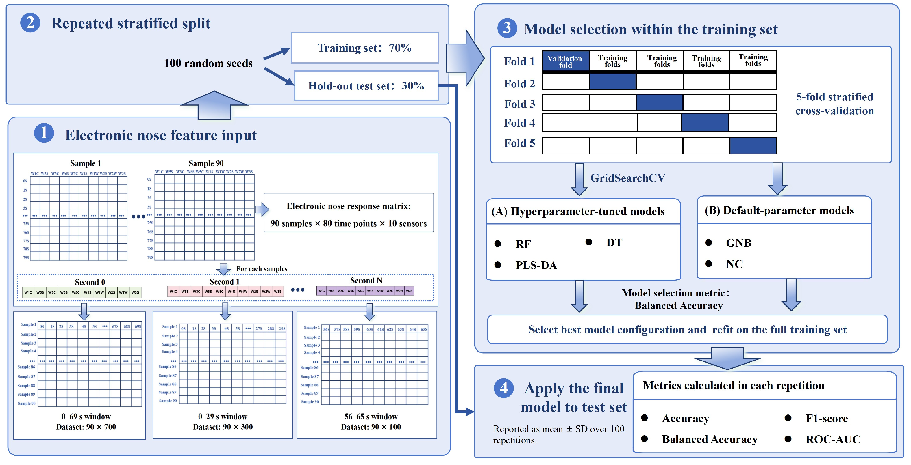
The overall model construction workflow is shown in Figure 1. E-nose response data were acquired from T. fuciformis samples. For each sample, raw response signals were recorded from ten sensors at 1 s intervals from 0 to 79 s, resulting in a 10 × 80 response matrix and 800 initial response variables. Three temporal-window feature sets were then constructed from the selected overall response, early response, and relatively stable response stages to compare their discriminative value for the rapid geographical-origin discrimination of T. fuciformis. The 0–69 s window was defined as the selected overall response stage to retain the major dynamic information from the initial response to the near-stable stage. The 0–29 s window was selected as the early response stage to capture rapid adsorption and initial MOS sensor responses. The 56–65 s window was selected as the relatively stable response stage because the sensor responses tended to approach a more stable level during this period. For each time window, the response values of the ten sensors were arranged sequentially according to time order and concatenated into a one-dimensional feature vector for each sample. Consequently, three temporal-window feature datasets were constructed, with dimensions of 90 × 700, 90 × 300, and 90 × 100, respectively.

2.3.2. Model Construction Procedure

PCA was performed on the z-score-standardized E-nose datasets to evaluate the overall data structure and the contribution of individual sensors. As an unsupervised multivariate method, PCA transforms high-dimensional sensor-response data into a lower-dimensional space defined by orthogonal principal components (PCs) [22,26]. PCA was therefore used for exploratory visualization of sample distribution and for assessing sensor contributions to the main variance structure.

To systematically evaluate the classification capability of E-nose features for geographical-origin discrimination, five classification models were selected: RF, PLS-DA, GNB, NC, and DT. These models represent different modelling strategies, including ensemble learning, linear discriminant modelling, probabilistic generative classification, distance-based classification, and tree-based classification. Their combined use enabled the separability of volatile-response patterns between T. fuciformis samples from different geographical origins to be assessed from multiple modelling perspectives.

RF is an ensemble classification method based on multiple decision trees. It builds multiple trees using resampled training data and randomly selected feature subsets, and the final class is determined by majority voting [27,28]. This strategy reduces the instability of a single decision tree and improves robustness when dealing with high-dimensional and nonlinear sensor-response data. PLS-DA is a supervised classification method derived from partial least squares regression. It converts class labels into numerical responses and extracts latent variables that capture the covariance between the sensor-response matrix and class information [29]. Because it can handle collinear and high-dimensional data, PLS-DA is widely used in chemometric analysis of spectral, E-nose, and metabolomic datasets [30]. GNB is a probabilistic classifier based on Bayes’ theorem. It estimates the probability that a sample belongs to each class by assuming that the features are conditionally independent and that continuous features approximately follow Gaussian distributions within each class [31,32]. NC is a distance-based classifier that represents each class by the mean feature vector of its training samples and assigns an unknown sample to the class with the nearest centroid. This model is simple and interpretable, and it can be used to evaluate whether different classes are separated in the overall sensor-feature space [33,34]. DT is a non-parametric classification method that recursively splits the feature space according to selected feature thresholds. The splitting process is usually guided by criteria such as the Gini index or entropy. DT can capture nonlinear classification patterns and is easy to interpret, but a single tree may be sensitive to changes in the training data and prone to overfitting. Therefore, model complexity was controlled by tuning parameters such as tree depth and the minimum number of samples in leaf nodes [35,36].

Algorithm-specific scaling was applied during model construction: PLS-DA, GNB, and NC were trained using z-score-standardized features, whereas RF and DT were trained without scaling because tree-based models are generally insensitive to feature scaling [37]. For each temporal-window dataset, model evaluation was performed using repeated stratified hold-out validation. Specifically, the samples were randomly divided into a training set and an independent test set at a ratio of 7:3 using stratified sampling, and this procedure was repeated 100 times with different random seeds to reduce the dependence of model performance on a single data partition. In each repetition, model training and hyperparameter optimization were performed only on the training set, whereas the hold-out test set was used only for final model evaluation. For models with tunable hyperparameters, including RF, PLS-DA, and DT, parameter optimization was conducted using 5-fold stratified cross-validation combined with GridSearchCV. Balanced accuracy was used as the model selection criterion to reduce the potential bias caused by class imbalance [38,39]. After the optimal hyperparameters were determined, each model was refitted using the complete training set of the corresponding repetition. Predictions were then made for both the training set and the independent test set. Accuracy, balanced accuracy, F1-score, and the area under the receiver operating characteristic curve (ROC-AUC) were calculated for each repetition, and the final performance of each model was reported as the mean ± standard deviation (SD) over the 100 repeated runs. Because these five supervised classification models are well-established machine learning methods, their theoretical principles are not further elaborated. RF, GNB, NC, and DT were implemented in Python using the scikit-learn package. For PLS-DA, class labels were encoded and modelled using partial least squares regression, followed by class assignment based on the predicted class scores.

2.3.3. Model Evaluation Metrics

Model performance was evaluated using accuracy, balanced accuracy, F1-score, and ROC-AUC [40]. Accuracy was used to describe the overall proportion of correctly classified samples. Balanced accuracy was calculated as the average recall across classes, thereby reducing the potential bias of ordinary accuracy toward the majority class under class-imbalanced conditions. In a binary classification task, balanced accuracy is equivalent to the arithmetic mean of sensitivity and specificity. The F1-score, defined as the harmonic means of precision and recall, was used to comprehensively evaluate the stability of target-class recognition. ROC-AUC represents the area under the ROC curve, in which the true positive rate (TPR) is plotted against the false positive rate (FPR), and was used to assess the overall ability of a model to distinguish between the two classes across different classification thresholds [41,42].

For binary classification, the confusion matrix consists of four outcomes: true positive (TP), true negative (TN), false positive (FP), and false negative (FN), as illustrated in Supplementary Figure S1. Specifically, TP and TN denote the numbers of positive and negative samples correctly classified, respectively, whereas FP and FN denote the numbers of negative samples misclassified as positive and positive samples misclassified as negative, respectively. Based on the confusion-matrix terms, sensitivity (recall or true positive rate, TPR), specificity (true negative rate, TNR), false positive rate (FPR), and precision were calculated as follows:

$$\mathrm{S}\mathrm{ensitivity}/\mathrm{Recall}/\mathrm{TPR} = {\displaystyle \frac{\mathrm{TP}}{\mathrm{TP}+\mathrm{FN}}},$$

(1)

$$\mathrm{Specificity}={\displaystyle \frac{\mathrm{TN}}{\mathrm{TN}+\mathrm{FP}}},$$

(2)

$$\mathrm{Precision}={\displaystyle \frac{\mathrm{TP}}{\mathrm{TP}+\mathrm{FP}}},$$

(3)

$$\mathrm{FPR}={\displaystyle \frac{\mathrm{FP}}{\mathrm{FP}+\mathrm{TN}}},$$

(4)

The four-evaluation metrics used in this study were calculated as follows:

$$\mathrm{Accuracy} = {\displaystyle \frac{\mathrm{TP}+\mathrm{TN}}{\mathrm{TP}+\mathrm{TN}+\mathrm{FP}+\mathrm{FN}}},$$

(5)

$$\mathrm{Balanced} \mathrm{Accuracy}={\displaystyle \frac{1}{2}}(\mathrm{Sensitivity}+\mathrm{Specificity})={\displaystyle \frac{1}{2}}\left({\displaystyle \frac{\mathrm{TP}}{\mathrm{TP}+\mathrm{FN}}}+{\displaystyle \frac{\mathrm{TN}}{\mathrm{TN}+\mathrm{FP}}}\right),$$

(6)

$$\text{F1-score}={\displaystyle \frac{2\times \mathrm{Precision}\times \mathrm{Sensitivity}}{\mathrm{Precision}+\mathrm{Sensitivity}}}={\displaystyle \frac{2\mathrm{TP}}{2\mathrm{TP}+\mathrm{FP}+\mathrm{FN}}},$$

(7)

$$\mathrm{AUC}={\int }_0^1\mathrm{TPR}\left(\mathrm{FPR}\right)d\left(\mathrm{FPR}\right),$$

(8)

ROC-AUC ranges from 0 to 1. An AUC value closer to 1 indicates stronger discriminative ability between the two classes, whereas an AUC value close to 0.5 suggests performance comparable to random guessing [41,43]. Accuracy, balanced accuracy, and F1-score all have an optimal value of 1. Under the same test set and evaluation settings, values closer to 1 generally indicate better classification performance [40].

3. Results and Discussion

3.1. Analysis of E-Nose Response Profiles

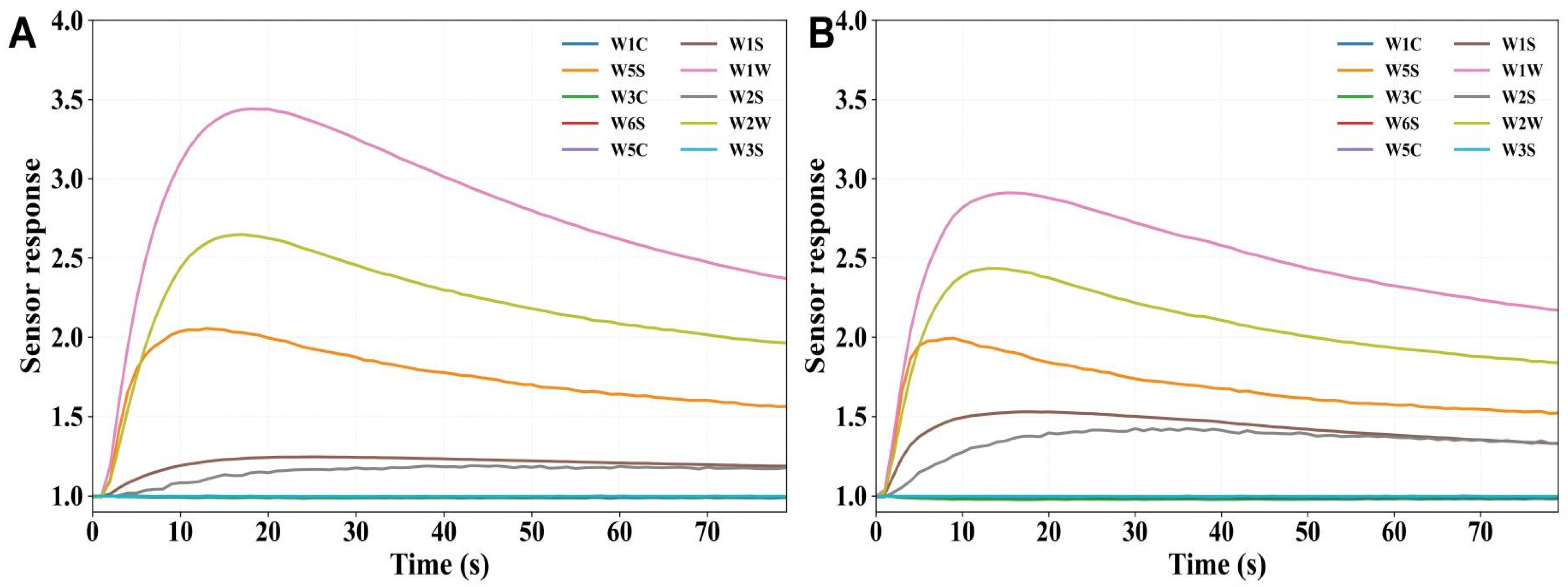
The PEN3 system used in this study is based on a commercial MOS sensor array. Although E-nose systems can also be developed using conducting polymer sensors, quartz crystal microbalance sensors, surface acoustic wave sensors, or nanostructured chemiresistive sensors [44,45]. MOS sensor arrays remain widely used in commercial instruments because of their low cost, rapid response, high sensitivity, robustness, and ease of integration. Figure 2 shows the temporal E-nose response fingerprints of T. fuciformis samples from the two geographical origins. Overall, the sensor responses of both groups exhibited clear time-dependent variation. The response signals increased rapidly during the initial stage of measurement, reached their maximum values after approximately 10–25 s, and then gradually decreased. This dynamic response pattern suggests that the volatile compounds released from T. fuciformis rapidly interacted with the MOS sensors during the early sampling stage. Subsequently, changes in headspace concentration distribution, together with adsorption–desorption processes on the sensor surface, caused the response signals to gradually stabilize or decline.

In terms of sensor response intensity, T. fuciformis samples from the two geographical origins exhibited broadly similar E-nose response patterns. In both groups, W1W, W2W, and W5S generated the most pronounced signals; W1S and W2S showed weaker responses; and W1C, W3C, W6S, W5C, and W3S remained close to the baseline. According to the typical response categories of the PEN3 sensor array, W1W is mainly associated with sulfur-containing organic compounds, W2W with sulfur- and chlorine-containing compounds, and W5S with broad-range compounds (Table 2). Therefore, the strong responses of W1W, W2W, and W5S indicate that these response channels were the main contributors to the E-nose odour fingerprint of T. fuciformis. By contrast, W1S and W2S are associated with broad methane and broad alcohol responses, respectively, and their weaker responses suggest that these two channels contributed less to the overall E-nose fingerprint. Furthermore, W1C and W3C are mainly associated with aromatic compounds, W6S with hydrogen, W5C with aromatic and aliphatic compounds, and W3S with methane and aliphatic compounds. The near-baseline responses of these sensors indicate that these specific response channels made limited signal contributions under the present sample condition [20,23]. This observation is partly in line with GC–MS evidence on the volatile profile of T. fuciformis. Hydrocarbons were detectable, whereas most saturated hydrocarbons occurred at relatively low abundances and had high odour thresholds, suggesting that they contributed only marginally to the overall aroma profile [8].

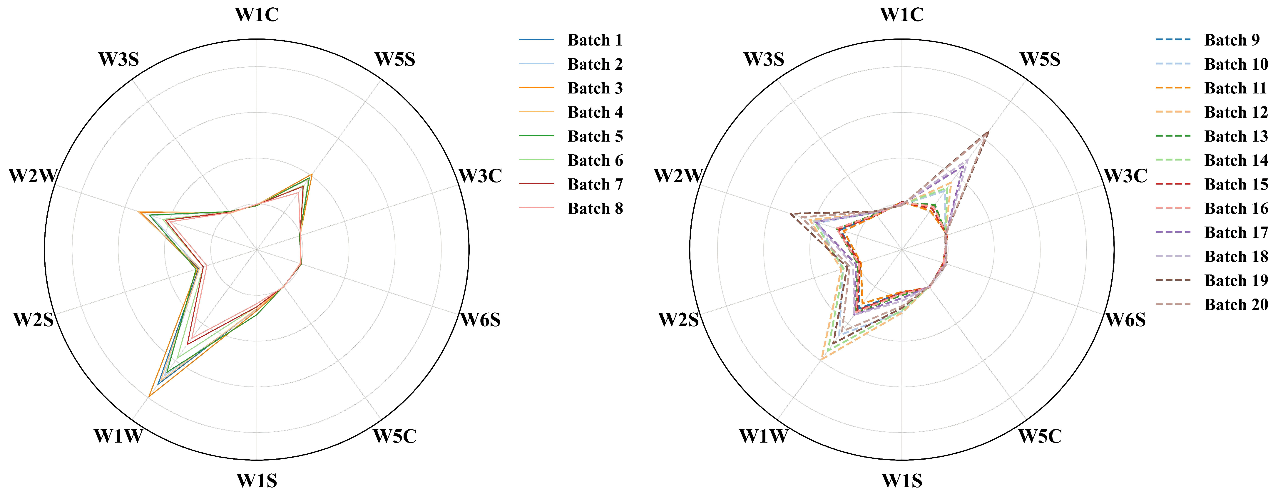
Based on the temporal response analysis, Figure 3 further presents the average radar plots of E-nose response fingerprints for different brands and batches of T. fuciformis samples at 65 s. The detailed data corresponding to Figure 3 was provided in Supplementary Table S1. The samples from each geographical origin comprised different commercial brands: batches 1–8 were from TJ and included Tianshenggui and Tongjiang Yiner, whereas the remaining batches were from GT and included Fudonghai, Fangjiapuzi, and Jintang. As shown in Figure 3, brand-related differences were observed, particularly in the strongly responsive sensors, including W1W, W2W, W5S, W1S, and W2S. For example, Tianshenggui showed stronger responses than Tongjiang Yiner, especially for W1W and W2W, although both brands exhibited a similar Tongjiang-related response pattern. Among the Gutian samples, Fangjiapuzi and Jintang showed partially overlapping profiles, whereas considerable batch-to-batch variation was observed within each brand. Despite these brand- and batch-related variations, the radar plots still revealed origin-related differences in the overall E-nose fingerprints. The major response directions were broadly similar between TJ and GT samples, but clear differences were observed in response intensity, profile compactness, and fingerprint coverage area. These results suggest that the geographical-origin discrimination of T. fuciformis depended more on the integrated response pattern of the sensor array than on the response of any single dominant sensor.

3.2. PCA

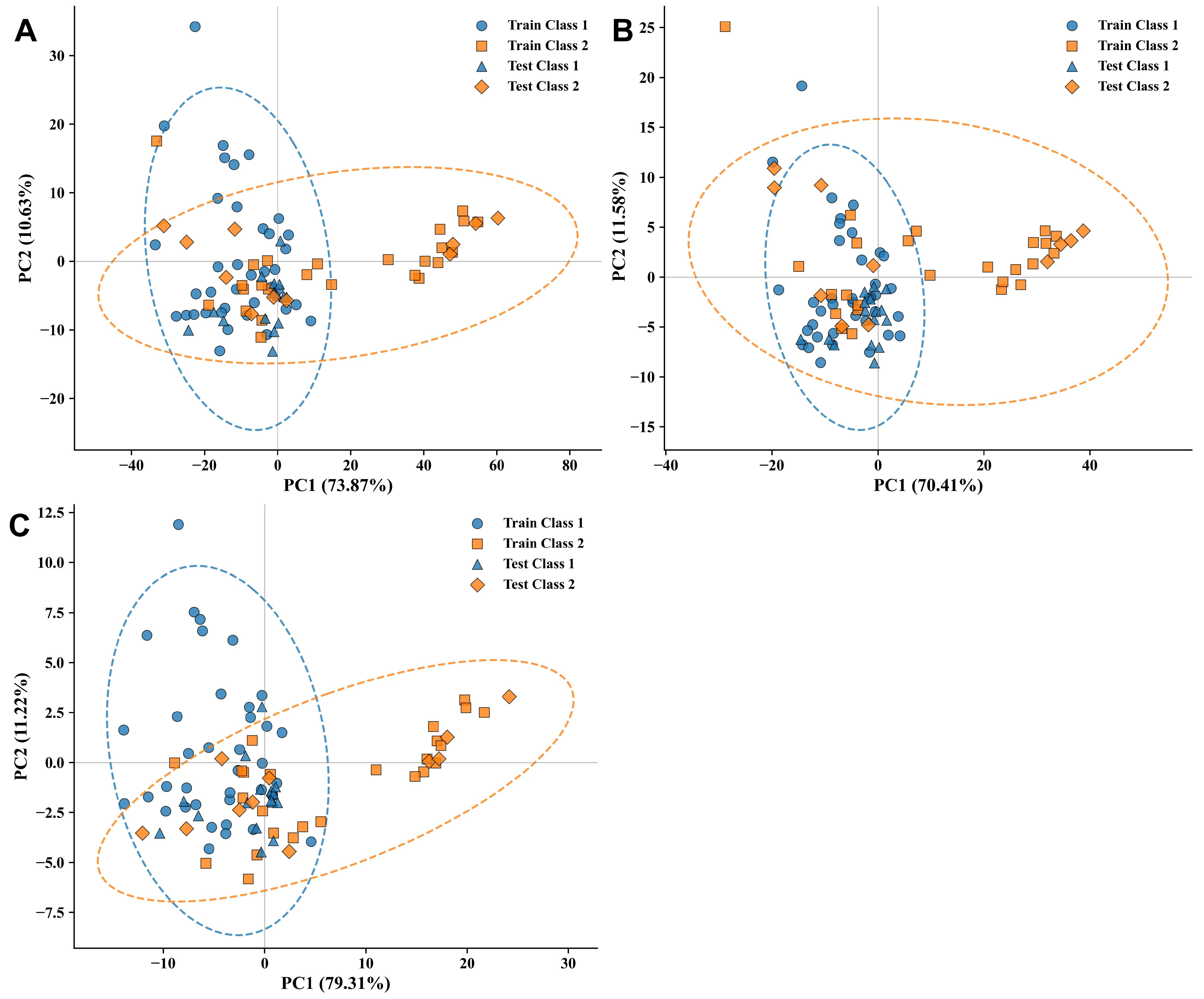
Figure 4 shows the PCA score plots constructed from E-nose features extracted from different time windows. For the 0–69 s feature set, PC1 and PC2 explained 73.87% and 10.63% of the total variance, respectively, with a cumulative explained variance of 84.50% (Figure 4A). For the early response window (0–29 s), the first two principal components explained 81.99% of the total variance (Figure 4B). The relatively stable response window (56–65 s) showed the highest cumulative explained variance, reaching 90.53% (Figure 4C), indicating that this window captured a larger proportion of the overall variance in the E-nose response data [46]. The PCA score plots showed a certain degree of distribution difference between the two geographical origins, particularly along PC1. In the 56–65 s feature set, part of the Class 2 samples tended to shift toward the positive PC1 region, whereas most Class 1 samples were distributed closer to the negative or central PC1 region. However, partial overlap between the two classes was still observed in all three PCA score plots, including the 56–65 s window. To further interpret the PCA results, the cumulative absolute loadings of the ten E-nose sensors on PC1 and PC2 were calculated for the three temporal-window feature sets (Supplementary Table S2). This loading analysis helped identify the sensors that contributed most strongly to the main variance structure of the E-nose fingerprints. In particular, W1W and W2W showed relatively high combined loading values in different temporal-windows, suggesting that these sensors played important roles in shaping the overall E-nose response patterns. This observation is consistent with previous E-nose-based research on T. fuciformis, in which PCA of sensor-response data explained 89% of the total variance using the first two principal components and revealed relatively concentrated and separated distributions among samples from four geographical origins [8].

3.3. Machine-Learning Results Based on Different Time Windows

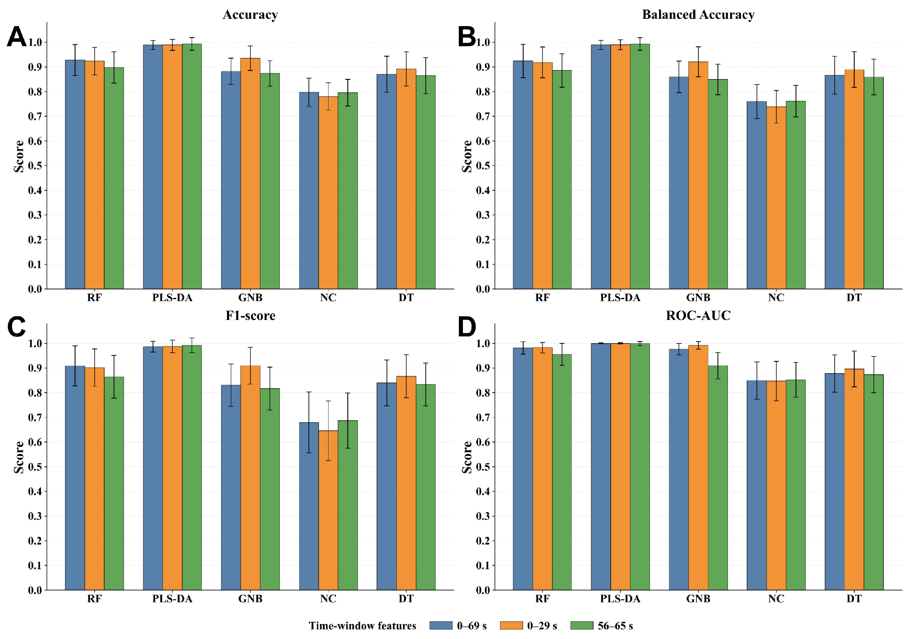
In this study, the TJ and GT groups contained 54 and 36 samples, respectively, representing a moderate class imbalance. To evaluate and reduce the potential influence of this imbalance, stratified sampling was used in each training–test split, balanced accuracy was used as the model-selection criterion during cross-validation, and accuracy, balanced accuracy, F1-score, ROC-AUC were reported. Moreover, the entire model evaluation procedure was repeated 100 times using different random seeds, and the results were reported as the mean ± standard deviation.

Table 3. The results of five classification models using different time windows.

Time Window	Model	Accuracy (Mean ± SD) 1	Balanced Accuracy (Mean ± SD)	F1-Score (Mean ± SD)	ROC_AUC (Mean ± SD)
0–69 s	DT	0.8704 ± 0.0732	0.8661 ± 0.0765	0.8397 ± 0.0929	0.8774 ± 0.0756
	GNB	0.8822 ± 0.0533	0.8596 ± 0.0636	0.8307 ± 0.0858	0.9763 ± 0.0230
	NC	0.7970 ± 0.0573	0.7593 ± 0.0691	0.6793 ± 0.1233	0.8494 ± 0.0758
	PLS-DA	0.9889 ± 0.0179	0.9892 ± 0.0182	0.9865 ± 0.0220	0.9997 ± 0.0019
	RF	0.9278 ± 0.0630	0.9240 ± 0.0676	0.9088 ± 0.0810	0.9810 ± 0.0248
0–29 s	DT	0.8919 ± 0.0692	0.8891 ± 0.0725	0.8668 ± 0.0874	0.8961 ± 0.0727
	GNB	0.9352 ± 0.0498	0.9210 ± 0.0605	0.9093 ± 0.0747	0.9918 ± 0.0150
	NC	0.7800 ± 0.0554	0.7385 ± 0.0662	0.6456 ± 0.1206	0.8471 ± 0.0799
	PLS-DA	0.9893 ± 0.0219	0.9899 ± 0.0202	0.9873 ± 0.0254	0.9997 ± 0.0023
	RF	0.9233 ± 0.0560	0.9181 ± 0.0626	0.9019 ± 0.0761	0.9823 ± 0.0215
56–65 s	DT	0.8644 ± 0.0732	0.8591 ± 0.0723	0.8335 ± 0.0869	0.8734 ± 0.0737
	GNB	0.8737 ± 0.0519	0.8491 ± 0.0621	0.8166 ± 0.0870	0.9095 ± 0.0534
	NC	0.7956 ± 0.0541	0.7614 ± 0.0635	0.6871 ± 0.1117	0.8521 ± 0.0704
	PLS-DA	0.9933 ± 0.0255	0.9928 ± 0.0256	0.9919 ± 0.0293	0.9991 ± 0.0085
	RF	0.8978 ± 0.0634	0.8853 ± 0.0680	0.8645 ± 0.0866	0.9553 ± 0.0447

¹ Values are reported as mean ± standard deviation over 100 random seeds.

shows the classification performance of five machine learning models using different time windows. Among the three windows, models based on the 0–29 s window achieved the best average performance, with the mean values across the five models for accuracy, balanced accuracy, F1-score, and ROC-AUC reaching 0.9039, 0.8914, 0.8622 and 0.9434, respectively. In particular, DT and GNB showed markedly better classification performance using the 0–29 s window features than using the other two temporal windows. This result may be attributed to the fact that the early response window (0–29 s) contains kinetic information related to the rapid release, transport, and adsorption of volatile compounds. Compared with the early response window (0–29 s), the selected overall response window (0–69 s) covered a broader portion of the E-nose response process and therefore retained more temporal information. With this feature set, NC and RF achieved better performance than their counterparts based on the 0–29 s window. However, this improvement was not observed consistently across the remaining classifiers. This may be because the broader response window introduced redundant variables, late-stage attenuation information, and potential sensor drift, thereby increasing feature dimensionality and model complexity [47]. For the relatively stable response window (56–65 s), the average model performance across the five models was the worst among the three temporal-window feature sets. Nevertheless, this window yielded the best performance for both PLS-DA and NC, suggesting that the relatively stable response stage may provide clearer class separation.

In terms of model performance, NC showed the weakest overall performance. Its accuracy ranged from approximately 0.7800 to 0.7970, balanced accuracy from 0.7385 to 0.7614, F1-score from 0.6456 to 0.6871, and ROC-AUC from 0.8471 to 0.8521 across the three temporal-window feature sets. A possible explanation for the weaker performance of NC is that the two groups of T. fuciformis samples may have shown substantial within-class dispersion and a relatively complex boundary in the E-nose feature space, rather than forming simple centroid-based clusters. Such a distributional pattern would be unfavorable for NC, which assumes that each class can be adequately represented by a single centroid [33]. Consequently, NC may have limited ability to capture synergistic or nonlinear variation among sensor responses.

In contrast, PLS-DA was the best-performing classifier across the three temporal-window feature sets. When using the 56–65 s feature set, PLS-DA achieved perfect classification performance, with accuracy, balanced accuracy, F1-score, and ROC-AUC reaching 0.9933 ± 0.0255, 0.9928 ± 0.0256, 0.9919 ± 0.0293, and 0.9991 ± 0.0085, respectively. Under the 0–29 s feature set, PLS-DA also outperformed the other classifiers, achieving accuracy, balanced accuracy, F1-score, and ROC-AUC values of 0.9893 ± 0.0219, 0.9899 ± 0.0202, 0.9873 ± 0.0254 and 0.9997 ± 0.0023, respectively. Rather than relying solely on accuracy, this study evaluated model performance using four complementary metrics, namely accuracy, balanced accuracy, F1-score, and ROC-AUC, to provide a more comprehensive assessment [10]. The high accuracy indicates good overall classification correctness, and the high balanced accuracy suggests that the model maintained comparable recognition ability for both classes. The high F1-score further indicates stable class-specific prediction performance with limited false-positive and false-negative errors [40]. In addition, the ROC-AUC value of 0.9991 demonstrates excellent threshold-independent discriminative ability between the two geographical origins [41]. These results indicate that the established PLS-DA model provided robust and balanced discrimination of T. fuciformis samples from the two origins. Previous studies have shown that multivariate analysis can differentiate T. fuciformis samples from different geographical origins. Elemental profiles combined with hierarchical clustering separated samples from two origins into distinct groups, whereas PCA of E-nose data showed relatively concentrated and separated distributions among samples from different origins [8,9]. However, hierarchical clustering and PCA are mainly unsupervised exploratory methods that reveal sample similarity, grouping trends, or variance structure rather than directly optimizing class discrimination. On the contrary, PLS-DA incorporates class-label information during model construction, thereby maximizing between-class separation and enabling quantitative prediction of independent samples. The superior performance of PLS-DA may be partly attributed to the high-dimensional, strongly correlated, and small-sample nature of the E-nose dataset. Under such data conditions, PLS-DA is particularly suitable because it projects high-dimensional temporal response variables onto a limited number of class-related latent variables, thereby retaining discriminative information while reducing the influence of multicollinearity among sensor responses [29].

As shown in Figure 5, the error bars, representing the standard deviation across 100 repeated stratified random splits, provide additional information on the robustness of different classifiers and temporal-window features. Overall, PLS-DA exhibited not only the highest mean performance but also the smallest variation across repeated runs. For all three temporal windows, the SD of accuracy, balanced accuracy, and F1-score were very small, and the ROC-AUC values were almost invariant. This indicates that the performance of PLS-DA was minimally affected by random training–test partitioning, suggesting strong robustness and stable extraction of discriminative information from the high-dimensional E-nose response features.

The results showed that PLS-DA effectively discriminates the moderately imbalanced TJ and GT groups. To examine whether class balancing further improved model performance, an additional sensitivity analysis was conducted using a randomly downsampled dataset. Specifically, 36 samples were randomly selected without replacement from the TJ group and combined with all 36 GT samples, resulting in a balanced dataset with 36 samples per class, as shown in Supplementary Table S2. Compared with the balanced-dataset models, the full-dataset PLS-DA model showed comparable or more stable performance, suggesting that the moderate imbalance did not compromise model robustness and may have helped preserve within-origin variability.

3.4. Analysis of Confusion Matrices

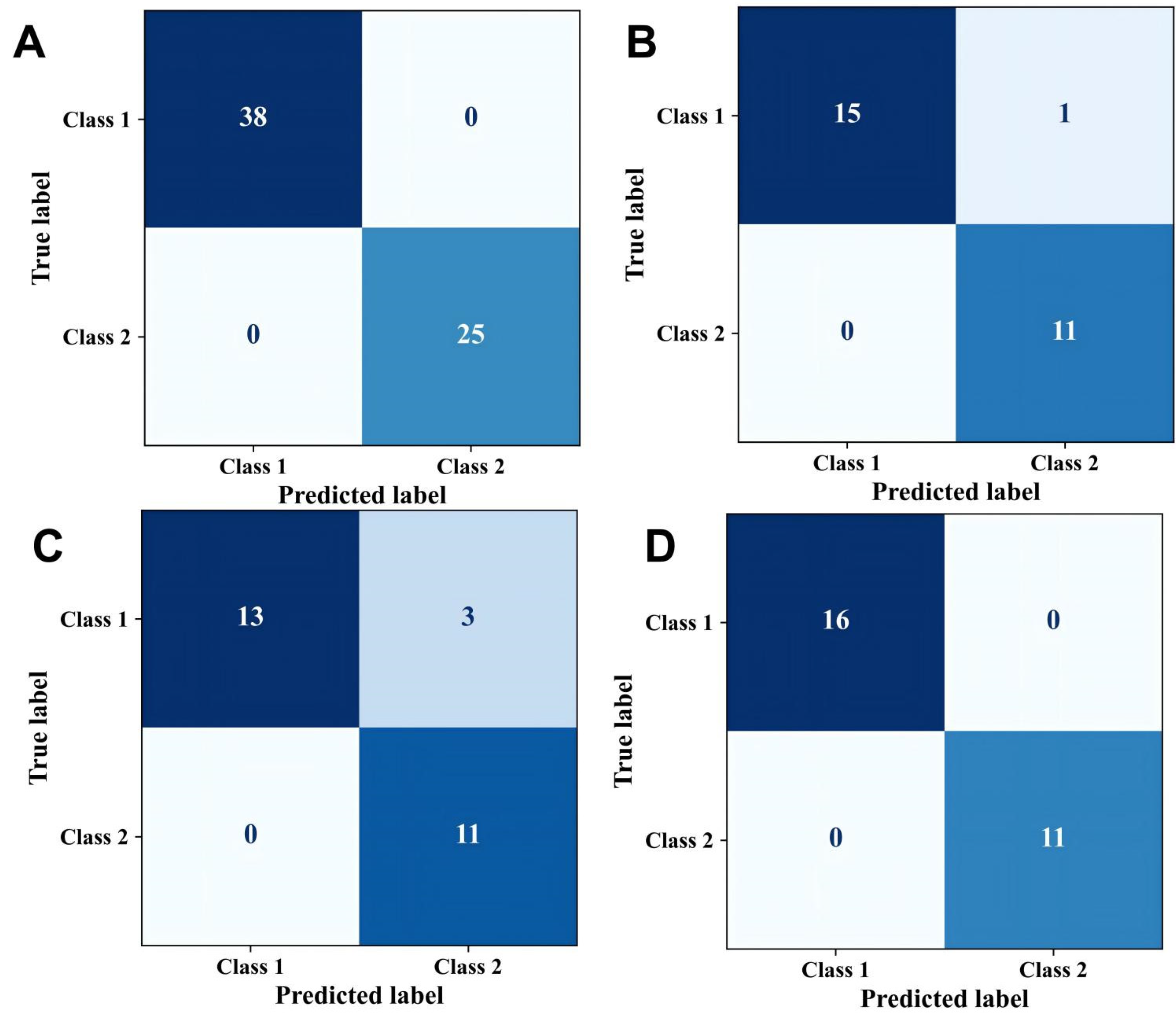
Although the evaluation metrics summarized the overall classification performance, confusion matrices were further examined to reveal class-specific prediction patterns and misclassification directions. This complementary analysis helped determine whether errors were concentrated in one geographical origin and provided direct evidence for assessing the reliability of the PLS-DA classification results. Figure 6 presents the confusion matrices of the PLS-DA model for different temporal-window feature sets. For this visualization, the training and hold-out test sets were generated using a stratified 7:3 split with random seed 81, and the same sample partition was applied to all temporal-window feature sets. In these matrices, Class 1 denotes T. fuciformis samples from TJ, whereas Class 2 denotes T. fuciformis samples from GT. Because the training-set classification results were identical across the 0–69 s, 0–29 s, and 56–65 s feature sets, only one representative training-set confusion matrix is presented in Figure 6A. The matrix indicates that PLS-DA correctly classified all 63 training samples, comprising 38 samples from Class 1 and 25 samples from Class 2.

For the test set, the classification performance differed among the three temporal-window feature sets. When the 0–69 s window features were used, the model correctly classified 15 Class 1 samples and 11 Class 2 samples, with only one Class 1 sample misclassified as Class 2. When the 0–29 s window features were used, the model correctly identified 13 Class 1 samples and all 11 Class 2 samples, whereas three Class 1 samples were misclassified as Class 2. By contrast, under the relatively stable window feature (56-65 s), all 16 Class 1 test samples and all 11 Class 2 test samples were correctly classified. This finding suggests that the relatively stable response window (56–65 s) more effectively captured the volatile-response differences between T. fuciformis samples from different geographical origins. In addition, in terms of misclassification patterns, all errors observed in the 0–69 s and 0–29 s test sets corresponded to Class 1 samples being predicted as Class 2, whereas no Class 2 samples were misclassified as Class 1. This pattern suggests that Class 2 samples had a relatively stable discriminant boundary in the latent-variable space extracted by PLS-DA, whereas some Class 1 samples may have shared similar E-nose response patterns with Class 2 samples.

3.5. Model Robustness and Overfitting Considerations

Because the E-nose temporal-window feature matrices were high-dimensional relative to the sample size, overfitting was considered a potential concern in this study, particularly for the 0–69 s and 0–29 s feature sets, which contained 700 and 300 variables, respectively, for 90 samples [30]. To reduce this risk, model optimization and performance evaluation were separated. For each random seed, the dataset was divided into a training set and a hold-out test set using stratified 7:3 splitting. The hold-out test set was not used for model training or hyperparameter optimization and was reserved only for final performance evaluation. For models with tunable hyperparameters, including RF, PLS-DA, and DT, parameter selection was performed only within the training set using 5-fold stratified cross-validation combined with GridSearchCV. Furthermore, the entire training–test splitting, model optimization, and evaluation procedure was repeated 100 times using different random seeds, and the final results were reported as the mean ± standard deviation rather than being based on a single data partition.

The PLS-DA model based on the 56–65 s feature window achieved accuracy, balanced accuracy, F1-score, and ROC-AUC values of 0.9933 ± 0.0255, 0.9928 ± 0.0256, 0.9919 ± 0.0293, and 0.9991 ± 0.0085, respectively. In addition, the relatively small SD across the 100 repeated splits indicates that the high classification performance was not driven by a single favorable training–test partition. Together with the use of independent hold-out test sets, these results suggest that the risk of overfitting was effectively reduced under the present validation strategy. The strong performance of PLS-DA is also consistent with a previous E-nose study in which LDA combined with five-window features achieved >99% accuracy in both validation and testing datasets, further supporting the value of supervised linear-discrimination models when combined with appropriate feature extraction and validation procedures [22].

However, some limitations are worth noting. Studies have shown that drying methods, including freeze drying, microwave drying, and hot-air drying, can affect the shrinkage ratio, rehydration ratio, microstructure, polysaccharide content, and free amino acid composition of instant T. fuciformis [48]. In addition, blanching treatments have been reported to influence the appearance, texture, sensory quality, polysaccharide content, and water migration characteristics of T. fuciformis [49]. This study was limited to two geographical indication production areas and commercially available dried products. Broader application will require validation using larger external datasets covering additional production regions, years, cultivation seasons, brands, processing batches, drying methods, and storage conditions. Such validation would provide a clearer assessment of the robustness and practical applicability of the model under more complex commercial scenarios.

4. Conclusions

This study characterized the E-nose fingerprints of T. fuciformis from TJ and GT and developed geographical-origin discrimination models using three temporal-window feature sets. The two origin groups showed distinguishable E-nose response patterns, with the main differences occurring in the strongly responsive sensors W1W and W2W. Among the evaluated feature sets and classification models, PLS-DA based on the 56–65 s response window achieved the best performance, with accuracy, balanced accuracy, F1-score, and ROC-AUC values of 0.9933 ± 0.0255, 0.9928 ± 0.0256, 0.9919 ± 0.0293, and 0.9991 ± 0.0085, respectively. These results indicate that the relatively stable E-nose response window provides informative fingerprint features for the rapid geographical-origin discrimination of commercial dried T. fuciformis products. The proposed method could serve as a rapid preliminary screening tool for quality control, market supervision, and food authentication. It requires only simple sample preparation and short instrumental analysis, without organic solvents or complex pretreatment procedures. Although the initial cost of the E-nose instrument should be considered, the relatively low per-sample cost may make this approach suitable for routine screening before confirmatory analysis.

References

1. Zhang, J.; Tong, Q.; Lin, F.; An, X.; Huang, H.; Chen, H.; Ye, J.; Xu, H.; Lv, X.; Lv, Z.; et al. Polymorphism and Evolutionary Origins of Accessory Chromosomes in the Basidiomycete Tremella fuciformis. Nat. Commun. 2026, 17, 3275. [Google Scholar] [CrossRef] [PubMed]
2. Li, S.; Zhao, K.; Li, J.; Li, X.; Zhao, H.; Cui, R.; Li, J.; Guo, J.; Bian, X. Recent Advances in Polysaccharides from Tremella fuciformis: Isolation, Structures, Bioactivities and Application. Front. Nutr. 2025, 12, 1663327. [Google Scholar] [CrossRef] [PubMed]
3. Sun, Y.; Syahariza, Z.A. Extraction, Structure, Biological Activities of Polysaccharides from Tremella fuciformis: A Review. J. Funct. Foods 2025, 133, 107012. [Google Scholar] [CrossRef]
4. Gitsomboon, S.; Ratanapornsompong, G.; Ongphiphadhanakul, B.; Thongpradit, S.; Chanprasertyothin, S.; Chailurtkit, L.; Nimitphong, H. Tremella fuciformis Beverage Improves Glycated Hemoglobin A1c and Waist Circumference in Overweight/Obese Prediabetic Subjects: A Randomized Controlled Trial. BMC Nutr. 2024, 10, 44. [Google Scholar] [CrossRef] [PubMed]
5. Zhang, L.; Chen, J.; Xu, F.; Han, R.; Quan, M.; Wang, L. Effect of Tremella fuciformis on Dough Structure and Rheology, Noodle Flavor, and Quality Characteristics. LWT 2022, 172, 114180. [Google Scholar] [CrossRef]
6. Lin, H.; Xiong, Q.; Huang, W.; Dai, X.; Yang, Y.; Huang, W.; Lai, S.; Sun, S.; Zhang, L. Analysis of Microbial Community Structure and Cultivation Performance Assessment in Tremella fuciformis Liquid Inoculum. J. Fungi 2025, 11, 825. [Google Scholar] [CrossRef] [PubMed]
7. Huang, S.; Zou, Y.; Ye, Z.; Chen, J.; Luo, J.; Lan, Y.; Guo, L.; Lin, J.; Zheng, Q. A Comparative Study on the Physio-chemical Properties, Antioxidant and Immuno-stimulating Activities of Two National Geographical Indication Products of Tremella fuciformis in China. Int. J. Food Sci. Technol. 2021, 56, 2904–2914. [Google Scholar] [CrossRef]
8. Fu, L.; Tian, J.; Liu, L.; Ma, Y.; Zhang, X.; Ma, C.; Kang, W.; Sun, Y. Analysis of Volatile Components in Tremella fuciformis by Electronic Nose Combined with GC-MS. J. Food Qual. 2022, 2022, 9904213. [Google Scholar] [CrossRef]
9. Li, M.; Jiang, C.; Cheng, Q.; Peng, M. Establishment of Element Fingerprint and Origin Identification of Tremella fuciformis by Inductively Coupled Plasma Mass Spectrometry. Chem. Anal. Meter. 2022, 31, 31–34. [Google Scholar] [CrossRef]
10. Du, G.; Liu, M.; Huang, L.; Su, Y.; Jiang, W. Quality Evaluation of Tremella fuciformis Polysaccharides from Different Sources. Chin. J. Exp. Tradit. Med. Formulae 2020, 26, 210–216. [Google Scholar] [CrossRef]
11. Tran, T.T.H.; Le, T.P.; Pham, N.H.; Lai, Q.D.; Hoang, Q.T.; Cung, T.T.Q.; Nguyen, H.D. Can You Taste the Place? Building Regional Sensory Standards for Black Pepper with GC-MS and Sensory Perception. Front. Food Sci. Technol. 2026, 5, 1672614. [Google Scholar] [CrossRef]
12. Fanning, E.; Eyres, G.; Frew, R.; Kebede, B. Linking Cocoa Quality Attributes to Its Origin Using Geographical Indications. Food Control 2023, 151, 109825. [Google Scholar] [CrossRef]
13. Lu, L.; Hu, Z.; Hu, X.; Li, D.; Tian, S. Electronic Tongue and Electronic Nose for Food Quality and Safety. Food Res. Int. 2022, 162, 112214. [Google Scholar] [CrossRef] [PubMed]
14. Zou, X.; Wang, C.; Luo, M.; Ren, Q.; Liu, Y.; Zhang, S.; Bai, Y.; Meng, J.; Zhang, W.; Su, S.W. Design of Electronic Nose Detection System for Apple Quality Grading Based on Computational Fluid Dynamics Simulation and K-Nearest Neighbor Support Vector Machine. Sensors 2022, 22, 2997. [Google Scholar] [CrossRef] [PubMed]
15. De Lima, A.C.; Aceña, L.; Mestres, M.; Boqué, R. A Rapid Method to Predict Beer Shelf Life Using an MS-Based e-Nose. Beverages 2024, 10, 11. [Google Scholar] [CrossRef]
16. Mutz, Y.S.; Maroum, S.M.; Tessaro, L.L.G.; De Oliveira Souza, N.; De Bem, M.M.; Alves, L.S.; Figueiredo, L.P.; Do Rosario, D.K.A.; Bernardes, P.C.; Nunes, C.A. Effectiveness of an E-Nose Based on Metal Oxide Semiconductor Sensors for Coffee Quality Assessment. Chemosensors 2025, 13, 23. [Google Scholar] [CrossRef]
17. Sánchez, R.; Díaz, F.; Melo, L. Portable MOS Electronic Nose Screening of Virgin Olive Oils with HS-SPME-GC-MS Corroboration: Classification and Estimation of Sunflower-Oil Adulteration. Chemosensors 2025, 13, 374. [Google Scholar] [CrossRef]
18. Kaushal, S.; Rana, P.; Chung, C.-C.; Chen, H.-H. Geographical Origin Classification of Oolong Tea Using an Electronic Nose: Application of Machine Learning and Gray Relational Analysis. Chemosensors 2025, 13, 295. [Google Scholar] [CrossRef]
19. Yan, J.; Guo, X.; Duan, S.; Jia, P.; Wang, L.; Peng, C.; Zhang, S. Electronic Nose Feature Extraction Methods: A Review. Sensors 2015, 15, 27804–27831. [Google Scholar] [CrossRef] [PubMed]
20. Wu, H.; Yue, T.; Xu, Z.; Zhang, C. Sensor Array Optimization and Discrimination of Apple Juices According to Variety by an Electronic Nose. Anal. Methods 2017, 9, 921–928. [Google Scholar] [CrossRef]
21. Yang, R.; Wang, Y.; Wang, J.; Guo, X.; Zhao, Y.; Zhu, K.; Zhu, X.; Zou, H.; Yan, Y. Geographical Origin Traceability of Atractylodis Macrocephalae Rhizoma Based on Chemical Composition, Chromaticity, and Electronic Nose. Molecules 2024, 29, 4991. [Google Scholar] [CrossRef] [PubMed]
22. Putri, L.A.; Rahman, I.; Puspita, M.; Hidayat, S.N.; Dharmawan, A.B.; Rianjanu, A.; Wibirama, S.; Roto, R.; Triyana, K.; Wasisto, H.S. Rapid Analysis of Meat Floss Origin Using a Supervised Machine Learning-Based Electronic Nose towards Food Authentication. npj Sci. Food 2023, 7, 31. [Google Scholar] [CrossRef] [PubMed]
23. Jia, W.; Liang, G.; Tian, H.; Sun, J.; Wan, C. Electronic Nose-Based Technique for Rapid Detection and Recognition of Moldy Apples. Sensors 2019, 19, 1526. [Google Scholar] [CrossRef] [PubMed]
24. Sun, M.; Ma, J.; Cai, Z.; Yan, J.; Ma, R.; Yu, M.; Xie, Y.; Shen, Z. Integrating Sensory Evaluation, Electronic Nose, and Metabolomics to Characterize Aroma in Peach and Nectarine Varieties. Foods 2025, 14, 3087. [Google Scholar] [CrossRef] [PubMed]
25. Li, B.; Gu, Y. A Machine Learning Method for the Quality Detection of Base Liquor and Commercial Liquor Using Multidimensional Signals from an Electronic Nose. Foods 2023, 12, 1508. [Google Scholar] [CrossRef] [PubMed]
26. Xu, W.; Zhang, C.; Xu, R.; Yang, J.; Kong, Y.; Liu, L.; Tao, S.; Wu, Y.; Liao, H.; Mao, C.; et al. E-Nose and HS-SPME-GC-MS Unveiling the Scent Signature of Ligusticum chuanxiong and Its Medicinal Relatives. Front. Plant Sci. 2025, 16, 1476810. [Google Scholar] [CrossRef] [PubMed]
27. Breiman, L. Random Forests. Mach. Learn. 2001, 45, 5–32. [Google Scholar] [CrossRef]
28. Breiman, L. Bagging Predictors. Mach. Learn. 1996, 24, 123–140. [Google Scholar] [CrossRef]
29. Barker, M.; Rayens, W. Partial Least Squares for Discrimination. J. Chemom. 2003, 17, 166–173. [Google Scholar] [CrossRef]
30. Ruiz-Perez, D.; Guan, H.; Madhivanan, P.; Mathee, K.; Narasimhan, G. So You Think You Can PLS-DA? BMC Bioinform. 2020, 21, 2. [Google Scholar] [CrossRef] [PubMed]
31. Wang, W.; Yan, L.; Liu, F.; Li, Y. Improving Gaussian Naive Bayes Classification on Imbalanced Data through Coordinate-Based Minority Feature Mining. PeerJ Comput. Sci. 2025, 11, e3003. [Google Scholar] [CrossRef] [PubMed]
32. Srisuradetchai, P. Posterior Averaging with Gaussian Naive Bayes and the R Package RandomGaussianNB for Big-Data Classification. Front. Big Data 2025, 8, 1706417. [Google Scholar] [CrossRef] [PubMed]
33. Dabney, A.R.; Storey, J.D. Optimality Driven Nearest Centroid Classification from Genomic Data. PLoS ONE 2007, 2, e1002. [Google Scholar] [CrossRef] [PubMed][Green Version]
34. Chopra, D.; Khurana, R. Introduction to Machine Learning with Python; Bentham Science Publishers: Singapore, 2023. [Google Scholar] [CrossRef]
35. Loh, W.Y. Classification and Regression Trees. WIREs Data Min. Knowl. Discov. 2011, 1, 14–23. [Google Scholar] [CrossRef]
36. Ahmed, A.M.; Rizaner, A.; Ulusoy, A.H. A Novel Decision Tree Classification Based on Post-Pruning with Bayes Minimum Risk. PLoS ONE 2018, 13, e0194168. [Google Scholar] [CrossRef] [PubMed]
37. Ahsan, M.; Mahmud, M.; Saha, P.; Gupta, K.; Siddique, Z. Effect of Data Scaling Methods on Machine Learning Algorithms and Model Performance. Technologies 2021, 9, 52. [Google Scholar] [CrossRef]
38. Brodersen, K.H.; Ong, C.S.; Stephan, K.E.; Buhmann, J.M. The Balanced Accuracy and Its Posterior Distribution. In Proceedings of the 2010 20th International Conference on Pattern Recognition, Istanbul, Turkey, 23–26 August 2010; IEEE: Piscataway, NJ, USA, 2010; pp. 3121–3124. [Google Scholar] [CrossRef]
39. Yates, L.A.; Aandahl, Z.; Richards, S.A.; Brook, B.W. Cross Validation for Model Selection: A Review with Examples from Ecology. Ecol. Monogr. 2023, 93, e1557. [Google Scholar] [CrossRef]
40. Sokolova, M.; Lapalme, G. A Systematic Analysis of Performance Measures for Classification Tasks. Inf. Process. Manag. 2009, 45, 427–437. [Google Scholar] [CrossRef]
41. Fawcett, T. An Introduction to ROC Analysis. Pattern Recognit. Lett. 2006, 27, 861–874. [Google Scholar] [CrossRef]
42. Bradley, A.P. The Use of the Area under the ROC Curve in the Evaluation of Machine Learning Algorithms. Pattern Recognit. 1997, 30, 1145–1159. [Google Scholar] [CrossRef]
43. Hanley, J.A.; McNeil, B.J. The Meaning and Use of the Area under a Receiver Operating Characteristic (ROC) Curve. Radiology 1982, 143, 29–36. [Google Scholar] [CrossRef] [PubMed]
44. Shooshtari, M.; Salehi, A. An Electronic Nose Based on Carbon Nanotube-Titanium Dioxide Hybrid Nanostructures for Detection and Discrimination of Volatile Organic Compounds. Sens. Actuators B Chem. 2022, 357, 131418. [Google Scholar] [CrossRef]
45. Sanislav, T.; Mois, G.D.; Zeadally, S.; Folea, S.; Radoni, T.C.; Al-Suhaimi, E.A. A Comprehensive Review on Sensor-Based Electronic Nose for Food Quality and Safety. Sensors 2025, 25, 4437. [Google Scholar] [CrossRef] [PubMed]
46. Jolliffe, I.T.; Cadima, J. Principal Component Analysis: A Review and Recent Developments. Philos. Trans. R. Soc. A Math. Phys. Eng. Sci. 2016, 374, 20150202. [Google Scholar] [CrossRef] [PubMed]
47. Wörner, J.; Eimler, J.; Pein-Hackelbusch, M. Long-Term Drift Behavior in Metal Oxide Gas Sensor Arrays: A One-Year Dataset from an Electronic Nose. Sci. Data 2025, 12, 1628. [Google Scholar] [CrossRef] [PubMed]
48. Li, Y.; Chen, J.; Lai, P.; Tang, B.; Wu, L. Influence of Drying Methods on the Physicochemical Properties and Nutritional Composition of Instant Tremella fuciformis. Food Sci. Technol. 2020, 40, 741–748. [Google Scholar] [CrossRef]
49. Zheng, Z.; Wu, L.; Li, Y.; Deng, W.; Chen, S.; Song, H. Effects of Different Blanching Methods on the Quality of Tremella fuciformis and Its Moisture Migration Characteristics. Foods 2023, 12, 1669. [Google Scholar] [CrossRef] [PubMed]
Figure 1. The overall model construction workflow. The ellipses (…) in the rows and columns denote the omission of intermediate, repeated samples or time points.
Chemosensors 14 00152 g001
Figure 2. Temporal response profiles of the E-nose sensor array for T. fuciformis samples from two geographical origins: (A) TJ; (B) GT.
Chemosensors 14 00152 g002
Figure 3. Average radar plots based on E-nose response fingerprints of T. fuciformis samples from different batches at 65 s.
Chemosensors 14 00152 g003
Figure 4. PCA score plots of T. fuciformis samples based on E-nose features extracted from different time windows: (A) 0–69 s; (B) 0–29 s; and (C) 56–65 s. The PCA was performed with a random seed of 81. Dashed ellipses indicate 95% confidence regions for each class in the training set.
Chemosensors 14 00152 g004
Figure 5. Performance comparison of machine-learning models using different time windows: (A) accuracy; (B) balanced accuracy; (C) F1-score; and (D) ROC-AUC.
Chemosensors 14 00152 g005
Figure 6. Confusion matrices of the PLS-DA model: (A) training set; (B) test set based on 0–69 s window; (C) test set based on 0–29 s window; and (D) test set based on 56–65 s window.
Chemosensors 14 00152 g006