Article

Geographical Origin Classification of Oolong Tea Using an Electronic Nose: Application of Machine Learning and Gray Relational Analysis

1
Department of Tropical Agriculture and International Cooperation, National Pingtung University of Science and Technology, Pingtung 91201, Taiwan
2
Department of Food Science, National Pingtung University of Science and Technology, Pingtung 91201, Taiwan
*
Author to whom correspondence should be addressed.
Chemosensors 2025, 13(8), 295; https://doi.org/10.3390/chemosensors13080295
Submission received: 21 June 2025 / Revised: 1 August 2025 / Accepted: 4 August 2025 / Published: 8 August 2025

Abstract

Taiwan accounts for 90% of the total oolong tea production and enjoys a good global reputation for its quality. In recent years, oolong tea from neighboring countries has been imported into Taiwan and sold as Taiwanese oolong at high prices. This study aimed to rapidly classify oolong tea from four geographical origins (Taiwan, Vietnam, China, and Indonesia) using an electronic nose (E-nose) combined with machine learning. Color measurements were also conducted to support the classification. The electronic nose (E-nose) was utilized to analyze the aroma profiles of tea samples. To classify the samples, five machine learning models—linear discriminant analysis (LDA), support vector machine (SVM), K-nearest neighbor (KNN), artificial neural network (ANN), and random forest (RF)—were developed using 70% of the dataset for training and tested on the remaining 30%. Gray relational analysis (GRA) was applied to measure the relationship between sensor responses and reference tea origins. Multivariate analysis of variance (MANOVA) indicated a statistically significant effect of tea origin on color parameters, as confirmed by both Pillai’s trace and Wilks’ Lambda (Λ) tests (p = 0.000 < 0.05). Among the tested models, LDA and ANN achieved the highest overall classification accuracy (98.33%), with ANN outperforming in the discrimination of Taiwanese oolong tea, achieving 98.89% accuracy. GRA presented higher gray relational grade (GRG) values for Taiwanese tea samples compared to other origins and identified sensors S4, S6, and S14 as the dominant contributors. In conclusion, the E-nose combined with machine learning provides a rapid, non-destructive, and effective approach for geographical origin classification of oolong tea.

1. Introduction

Globally, tea (Camellia sinensis) is the most frequently consumed non-alcoholic drink after water [1,2]. It is recognized for its refreshing taste and health-promoting compounds. These include polyphenols, catechins, theanine, and amino acids, which play a role in preventing oxidation, cardiovascular disease, chronic gastritis, etc. [3,4]. Global tea consumption is projected to experience significant growth, with market value expected to reach USD 148.16 billion by 2027, driven by a compound annual growth rate (CAGR) of 6.4%. This rapid growth emphasized the need for stringent quality control measures to improve tea quality in order to meet customer satisfaction and maintain market competitiveness [4].
Oolong tea is known for its distinct floral aroma and refined fruity taste, distinguishing it from unfermented green tea and fully fermented black tea [5,6,7]. In recent years, the global demand for consumption of oolong tea has increased, leading to its production in other countries, including South Korea, Japan, Sri Lanka, Myanmar, Thailand, Indonesia, China, and Vietnam [7,8]. One of the key qualitative attributes influencing the market value of oolong tea is its aroma. Studies indicate that the aroma characteristics of oolong tea are directly influenced by cultivar selection and processing techniques [9]. Additionally, other geographical and environmental factors, such as growing regions, cultivation methods, and tea varieties, also contribute significantly to the distinct aroma and flavor of tea. This is why famous teas worldwide are often named after their places of origin. Similarly, the quality characteristics of oolong tea vary across different growing regions, highlighting the influence of growing environment on its overall profile [7].
Taiwan produces a diverse range of famous teas due to its distinct geographical and environmental conditions of tea production [10]. Among them, Taiwanese oolong tea, particularly those cultivated in high mountain regions, is considered among the most expensive and highly valued teas in the world [11,12]. Oolong tea accounts for 90% of Taiwan’s total production, while black and green teas account for the remaining 10%. In 2015, only 30% of the oolong tea produced was exported, with the majority of 70% being consumed domestically. The same report also highlights Taiwan’s increasing dependence on imported tea alongside a decline in tea exports [12]. Over the past decade, oolong tea from China, Vietnam, and Indonesia has been increasingly produced using similar processing techniques to those of Taiwanese oolong tea. These imported teas are often sold in Taiwan as Taiwanese oolong tea at high prices, despite lacking authentic origin. Even tea experts find it challenging to differentiate between authentic and fake Taiwanese oolong tea based on its color, appearance, and texture alone. Such fraudulent practices not only mislead consumers but also damage the reputation of superior tea brands. Therefore, reliable and rapid methods for discriminating the geographical origin of oolong tea are essential to ensuring the authenticity, quality, and safety of Taiwanese tea [8].
Traditionally, the tea quality is assessed through sensory evaluation, which relies on color, taste, aroma, and appearance. This method requires trained evaluators, introducing subjectivity into the evaluation process. Individual evaluators may interpret tea characteristics differently based on their personal experiences, mood, and physiological state, affecting the method’s reliability [4]. In recent years, conventional analytical methods, including liquid chromatography–mass spectrometry (LC–MS), gas chromatography–mass spectrometry (GC–MS), high-performance liquid chromatography (HPLC), capillary electrophoresis (CE), micellar electrokinetic chromatography, inductively coupled plasma atomic emission spectrometry (ICP–AES), inductively coupled plasma mass spectrometry (ICP–MS), hyperspectral imaging, fluorescent probes, and near-infrared reflectance spectroscopy (NIRS), have been employed for tea quality analysis [2,4,8]. However, these techniques are time-consuming, require complex sample pre-treatments, involve high instrumental and operational costs, and demand skilled technicians [3]. As a promising alternative approach, the electronic nose (E-nose), designed to mimic biological olfactory processes, has emerged as a novel intelligent sensory technology [13]. This device comprises a gas sensor array for odor detection and a data processing unit for analysis [14]. Owing to its advantages of rapid and non-destructive detection, the E-nose, combined with machine learning methods, has been successfully applied in tea classification based on geographical origin, fermentation methods, chemical component analysis, quality grading, and storage evaluation conditions [3].
This study aims to classify Jin Xuan oolong tea from four geographical origins using an E-nose. To compare classification performance, five machine learning models were implemented: linear discriminant analysis (LDA), support vector machine (SVM), K-nearest neighbor (KNN), artificial neural network (ANN), and random forest (RF). Additionally, gray relational analysis (GRA) was used to analyze E-nose responses and identify the most relevant sensors for discriminating oolong tea from Taiwan.

2. Materials and Methods

2.1. Experimental Samples

Jin Xuan oolong tea leaf samples from the four geographical origins, including Taiwan (Nantou), Vietnam (Bao Loc), China (Fujian), and Indonesia (Sumatra), were selected as experimental samples in this study. All dried tea leaf samples were provided by Tong Shii Industrial Co., Ltd., a tea factory located in Taoyuan, Taiwan, in May 2022. There were 24 samples in each group; in total, 288 independent tea samples (24 sample types × 4 groups × 3 replicates) were employed in the experiments. The samples were packed, sealed, and stored in a refrigerator at 4 °C before testing.

2.2. Colorimetric Analysis

Color measurement was performed using a colorimeter (X-Rite Pantone, Grand Rapids, MI, USA). The color coordinates were determined based on the CIELAB color space system. The results were expressed as L* (lightness; values from 0 (black) to 100 (white)), a* (redness; positive and negative values indicate red and green), and b* (yellowness; positive and negative values indicate yellow and blue) [15].

2.3. E-Nose Instrument Set Up

A commercial Sextant electronic nose (Enosim Bio-Tech Co., Ltd., Hsinchu, Taiwan) was employed in this study. The system consisted of four main components: (a) a sensing chamber equipped with a gas sensor array, (b) a micropump integrated with a solenoid valve, (c) an adsorbent unit, and (d) auxiliary sensors for monitoring temperature and humidity (Figure 1). The sensor array included 14 metal oxide semiconductor (MOS) gas sensors, incorporating TGS (Taguchi gas sensor) series (Figaro USA, Inc., Arlington Heights, IL, USA), as well as SB and SP series (Nissha FIS, Inc., Osaka, Japan) sensors. As listed in Table 1, the target gases of the sensors range from alcohols to various volatile organic compounds (VOCs). The micropump and valve in the sampling system regulate and control the flow of ambient air (reference gas) and the sample gas that is pumped into the sensor chamber. Besides sampling and the gas sensor array, the E-nose is equipped with a crucial unit called the data acquisition (DAQ) system (Figure 1). The electric signals are carried to a DAQ system through an electric circuit, which subsequently transmits the data to a computer.

2.3.1. E-Nose Tea Sample Measurement

For each analysis, 6 g of tea samples was taken in a 50 mL beaker, covered with aluminum foil, and allowed to stand undisturbed for 60 min to allow headspace volatiles to accumulate. The resulting headspace gas was then directed through a Teflon tube into the gas sensor chamber at a constant flow rate of 0.4 L/min, where it interacted with metal oxide semiconductor (MOS) sensors. All experiments were conducted at a temperature of 25 ± 1 °C and air relative humidity of 40 ± 5%.
To achieve a steady-state sensor response, the E-nose was preheated for 30 min prior to sample measurement. The total duration of the gas measurement was 850 s, and the measurement process consisted of three phases, namely reference baseline, collection, and recovery (Supplementary Information, Figure S1). During the reference baseline phase (100 s), the micropump drew ambient air from the reference connector into the sensor chamber to establish a baseline. In the collection phase (150 s), the aroma of the tea sample was pumped into the sensor chamber from the sample container, interacting with the sensor array to provide a range of response signals and returning to a stable baseline. Finally, during the recovery phase (600 s), the ambient air was passed into the sensor chamber, ensuring stabilized sensor responses.

2.3.2. Data Acquisition and Feature Extraction

A USB-6009 DAQ card (National Instruments Corporation, Austin, TX, USA) was used for data acquisition in this study. The Meta Editor of the ESRTSD program was used for exporting experimental data in CSV format on the computer. The typical sensor resistance responses were obtained from 14 E-nose sensors (S1–S14) during exposure to the tea sample aroma. Five subdivisions of the E-nose data, performed to extract resistance responses per sensor, were used as feature inputs for machine learning models.

2.4. Unsupervised Principal Component Analysis (PCA)

PCA is the most widely employed unsupervised learning algorithm to reduce the dimensionality of data through orthogonal transformation into principal components (PCs). These are new sets of variables (uncorrelated) that are linearly related to the original sets of variables (correlated). PCA is particularly useful for identifying the variations and similarities among different samples [16]. According to the Kaiser criterion, only PCs with eigenvalues greater than 1 are considered significant and retained in the analysis [3].

2.5. Machine Learning Models

The key concept behind a machine learning-based predictive model is to develop the model using trained data, which is then employed in predicting the results using new data [17]. Although these methods are generally less interpretable, they can handle various types of data, provide greater flexibility, and effectively capture complex relationships between response variables and predictors. As a result, they often deliver higher predictive accuracy, resulting in improved sample prediction performance [11].
In this study, the data was divided into a training set (70%) and a testing set (30%). The training set was used to build the classification model. The testing set was used to evaluate the accuracy of the model developed from the training data.

2.5.1. Linear Discriminant Analysis (LDA)

LDA is a supervised learning algorithm, which is a generalization of Fisher’s linear discriminant [18,19]. It is widely used in machine learning to identify a linear combination of features that characterizes or distinguishes between two or more classes of objects. It takes into account information about both the within-class and between-class distributions and projects high-dimensional data onto a low-dimensional space, maximizing class separability [19]. The LDA performs this transformation through three main steps: (1) calculating between-class variance, (2) calculating within-class variance, and (3) creating a lower-dimensional space that minimizes within-class variance while maximizing between-class variance [20].

2.5.2. Support Vector Machine (SVM)

SVM is one of the most widely recognized machine learning algorithms in supervised learning, utilized for binary-class classification problems [21]. This algorithm works by identifying the hyperplane that provides the training samples with the maximum margin. The optimal separating hyperplane, therefore, maximizes the margin of the training data. For non-linear separable classification problems, SVM transforms the original space into a higher-dimensional space by applying a kernel function. Thus, a hyperplane is built in the higher-dimensional space to solve the non-linear separable classification problems in the original low-dimensional space. The radial basis function (RBF), sigmoid, linear, and polynomial kernels are the four most well-known types used [22].

2.5.3. K-Nearest Neighbor (KNN)

The KNN is a supervised machine learning algorithm that is simple to understand and use. Unlike many other algorithms, KNN does not build a classification model. Instead, it stores the entire training dataset during the training phase. [21]. It presents a prediction target, determines the distance or similarity between the predicted target and samples, chooses the first k samples that are nearest to each other, and then utilizes those samples to select a decision based on the majority of k votes. Euclidean distance is a popularly used distance metric for calculating the interpoint distances between samples and is considered effective for clustering data [16].

2.5.4. Artificial Neural Network (ANN)

ANN is a powerful machine learning algorithm capable of non-linear mapping [23]. Typically, an ANN system is structured into three main layers or components, namely, the input layer, the hidden layer, and the output layer. The number of nodes in the input layer represents the number of variables (attributes) being analyzed. The number of neurons in the output layer represents the total number of target classes. The number of hidden layers and the number of neurons are determined based on the task’s complexity and the size of the training dataset. Each neuron in the hidden and output layers is connected to all the nodes in the preceding layer through associated numerical weights. These weights control the strength of the signal passing between neurons [24].

2.5.5. Random Forest (RF)

RF is an ensemble machine learning algorithm that aggregates several decision trees into a forest for prediction [17,25]. Firstly, N bootstrap samples are taken from the original training dataset to build a RF. Then, unpruned classification or regression trees are constructed for each bootstrap sample with the modifications as follows: at every node, a random sample m (m < M) of predictors (each sample consists of M predictors) is picked, and the best split among those variables is selected. The second step is repeated until the node can no longer be divided without pruning. The generated decision trees are finally combined into a random forest, which is then used for classification or regression of new data [26].

2.5.6. Model Evaluation Metrics

To assess the performance of supervised machine learning models, a set of metrics was evaluated. Common metrics used include accuracy, error rate, precision, recall (sensitivity), specificity, and F1 score [17,27]. The confusion matrix provided the True Positive (TP), False Positive (FP), True Negative (TN), and False Negative (FN) parameters for calculating the metrics in Equations (1), (2), (3), (4), (5), and (6), respectively.
A c c u r a c y = ( T P + T N ) / ( T P + T N + F P + F N )
E r r o r   r a t e = 1 A c c u r a c y
P r e c i s i o n = T P / ( T P + F P )
R e c a l l = T P / ( T P + F N )
S p e c i f i c i t y = T N / ( F P + T N )
F 1 = 2 ( P r e c i s i o n × R e c a l l ) / ( P r e c i s i o n + R e c a l l )

2.6. Gray Relational Analysis (GRA)

GRA, developed by Deng [28], is a comparative and optimization method based on the gray system theory. This approach is particularly useful for simplifying the model factors by addressing the complicated interrelationships among the multiple attributes while simultaneously calculating the gray relational grade (GRG) [29]. Here, for this study, the geographical tea origins (Taiwan, Vietnam, China, and Indonesia) and E-nose sensors (S1–S14) were introduced as a gray system. According to the literature [29,30,31], the GRA procedure involves several steps as follows.
The first step included linear normalization of the raw data. This step, known as data pre-processing, was performed using Equation (7).
     X t ( k ) = x t k min x t t ( k ) max x t t ( k ) min x t t ( k )
where X t k represents the normalized value, m i n x t ( k ) is the minimum value at the primary level, m a x x t ( k ) is the maximum value at the primary level, t denotes the trial number, and k = 1 to 4.
The second step calculated the deviation sequences, denoted as Δ x i k (i = 1 to 14) in Equation (8).
Δ x i k = | X i ( k ) X 0 ( k ) |
The third step determined the gray relational coefficients (GRCs), shown in Equation (9).
Y i ( k ) = min i   min k   Δ x i ( k ) + μ   max i   max k   x i ( k ) x i ( k ) + μ   max i   max k   x i ( k )
where Y i ( k ) represents GRC, min min x i ( k ) refers to the minimum value at the second level, max max x i ( k ) is the maximum value at the second level, and μ is the distinguishing coefficient with an assigned value of 0.5.
The fourth step calculated the GRG value, which accounted for an average sum of GRC in Equation (10).
γ i = 1 n k = 1 n Y i ( k )
where γ i refers to GRG, while n represents the number of GRC values.
Following the above equations, the GRC values and their corresponding GRG values were determined. By comparing the GRG values, the influence degree of comparison sequences on reference sequences was assessed. A higher GRG value indicated a stronger correlation degree [30].

2.7. Software

A one-way multivariate analysis of variance (MANOVA) was performed using SPSS Statistics (version 22.0) to evaluate whether the color parameters significantly varied among teas from different origins. Additionally, a radar chart was generated using Microsoft Excel 365 (Microsoft Corporation, Redmond, WA, USA) to visually compare the color profiles. PCA was performed using SPSS Statistics (version 22.0). Machine learning classification models were developed using SPSS Modeler (version 3.5.1). GRA was applied in the open-source programming language Python (version 3.10) to evaluate the gray relation degree and coefficient.

3. Results and Discussion

3.1. Descriptive Statistics and Multivariate Tests for Color Analysis

As shown in Table 2, the L* values of oolong tea samples were highest for those from China (26.91 ± 4.13) and lowest for samples from Taiwan (19.86 ± 0.87). No significant differences in L* values were observed between samples from Indonesia (22.35 ± 3.56) and Vietnam (22.18 ± 1.86). The highest a* values were recorded for samples from Vietnam (2.08 ± 0.50) and Indonesia (1.99 ± 0.42), followed by Taiwan (1.24 ± 0.37) and China (0.52 ± 0.29). Conversely, samples from Indonesia (13.43 ± 2.22) exhibited the highest b* value, while those from Taiwan (9.47 ± 0.87) had the lowest. Samples from Vietnam (11.94 ± 2.49) and China (11.43 ± 2.07) showed similar b* values. These findings highlight the distinct color characteristics of tea samples, particularly those from Taiwan, distinguishing them from other origins.
The significant differences in L*, a*, and b* values reflect distinct visual profiles among tea samples from different origins. For instance, the lower L* and b* values of Taiwanese tea samples indicate a darker, less yellow hue, which helps differentiate them from teas of other origins. Such variations in color parameters support their use as effective indicators for origin-based classification.
A recent study [32] used Pillai’s trace and Wilks’ Λ as the preferred test statistics for MANOVA. Therefore, we selected these two tests to examine the multivariate significant effects of dependent variables (color parameters) on independent variables (tea origins). In Table 3, the analysis showed statistically significant multivariate effects of color parameters among the tea origins as indicated by Pillai’s trace (F (9, 852) = 71.868, p = 0.000 < 0.05; Pillai’s trace = 1.295, partial η2 = 0.432) and Wilks’ Λ (F (9, 686.465) = 114.982, p = 0.000 < 0.05; Wilks’ Λ = 0.107, partial η2 = 0.526) tests.

3.2. E-Nose Results

3.2.1. E-Nose Sensor Response

The E-nose response revealed distinct response signal characteristics for each type of tea sample based on their origins. The aromas of tea samples detected by gas sensors were converted into electrical signals (resistance), reflecting sensor response. As a whole, the sensor responses in Figure 2a–d of the tea samples from the four origins demonstrated similarities in resistance response patterns. However, the differences were seen in the responses of specific sensors: S14, S9, S10, and S11.
As illustrated in Figure 2, S14 exhibited the strongest response across the four origins, with resistance values of 4.41 Ω for samples from China, 4.37 Ω from Indonesia, 3.94 Ω from Taiwan, and 3.90 Ω from Vietnam. For sensors S9, S10, and S11, distinct patterns were observed. In samples from China, the resistance values for S9, S10, and S11 were 3.50 Ω, 3.42 Ω, and 3.40 Ω, respectively. Conversely, samples from Vietnam followed a different trend, with S10, S9, and S11 displaying resistance values of 3.58 Ω, 3.54 Ω, and 3.53 Ω, respectively. In samples from Indonesia and Taiwan, S9 showed a similar response of 3.48 Ω, whereas S10 and S11 exhibited weaker responses, with resistance signals below 3.40 Ω. These variations in sensor responses highlight distinct aroma profiles among the tea samples from the four origins.

3.2.2. E-Nose Aroma Fingerprint

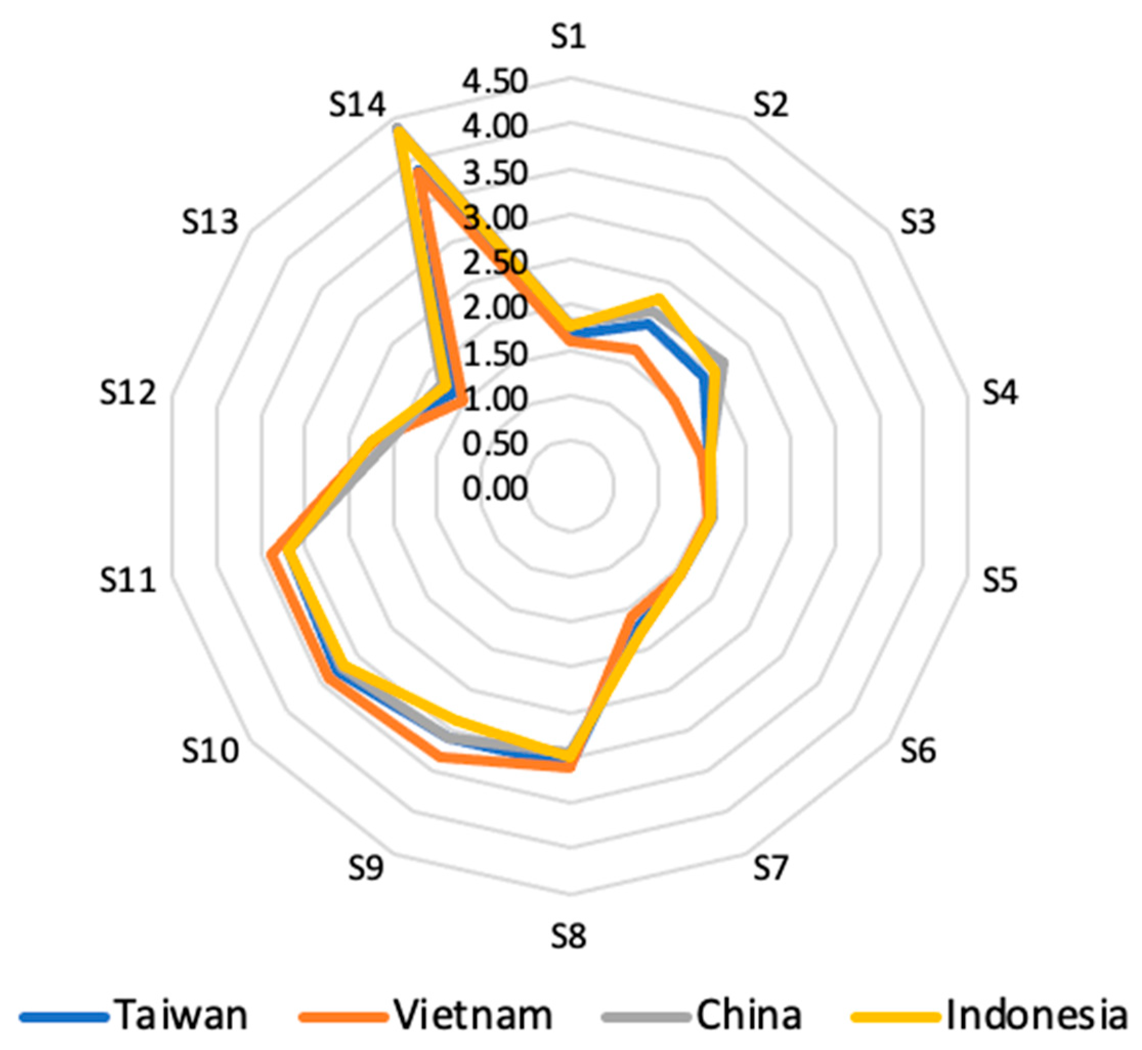
To gain a more comprehensible understanding of the data collected from the E-nose, the average sensor response values were calculated and illustrated in the radar chart shown in Figure 3. The chart reveals four patterns, each corresponding to oolong tea samples from different geographical origins: Taiwan, Vietnam, China, and Indonesia. Although the sample patterns (fingerprint aromas) exhibit overlap, some differences can be observed in specific sensors. Notably, sensor S14 exhibited the highest sensitivity across all four origins, with particularly strong signals for samples from Indonesia and China, followed by Taiwan and Vietnam. It is worth mentioning that sensor S14 is highly capable of detecting ozone, nitrogen oxides, and volatile organic compounds, making it highly responsive to certain tea volatiles. However, due to the complex and diverse chemical composition of oolong tea, interpreting results solely based on radar plot patterns may lead to inaccurate conclusions. Therefore, further application of machine learning methods to the multidimensional E-nose data is recommended to improve the classification and discrimination of oolong tea based on geographical origin.

3.3. PCA of Sensor Data

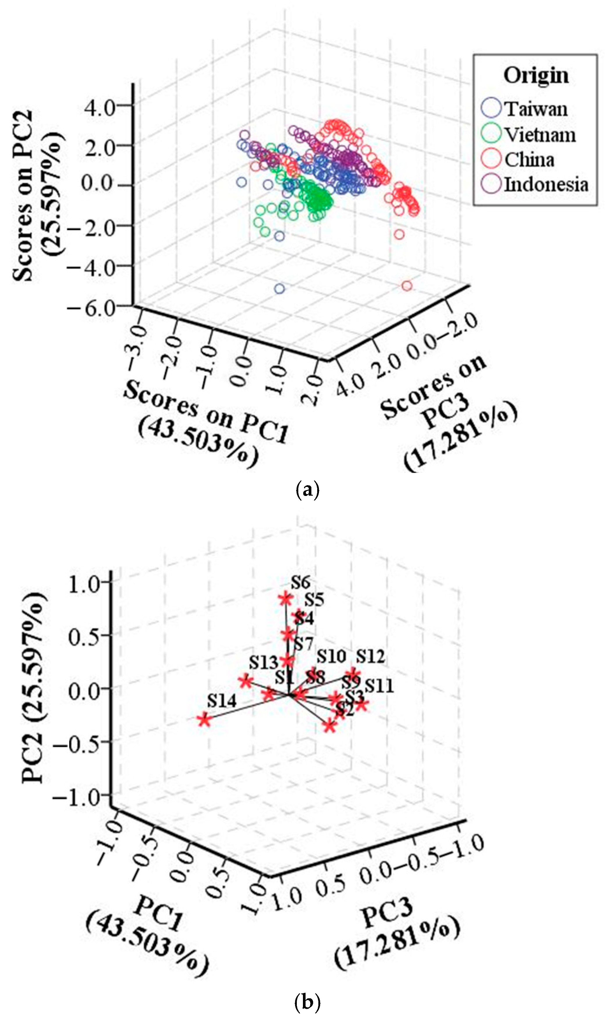
The projections of the first three principal components (PCs) extracted through PCA for the tea groups are illustrated in Figure 4a. The x-axis represents PC1, explaining 43.503% of the variance, while the y-axis and z-axis correspond to PC2 and PC3, accounting for 25.597% and 17.281% of the variance, respectively. Together, these three PCs accounted for 86.381% of the cumulative variance, indicating a greater degree of information loss. A three-dimensional (3-D) score plot (Figure 4a) shows the classification of tea samples from four geographical origins. Samples that are clustered together exhibit similar response patterns, whereas those farther apart contribute distinct variations. All the formed clusters are closely positioned with each other with noticeable overlap, suggesting that PCA alone may not provide high classification accuracy. This highlights the need for more advanced classification approaches, such as machine learning, to achieve greater accuracy for tea classification.
The PCA loading plot is presented in Figure 4b, where 14 vectors represent 14 sensors (S1–S14). The contribution of each sensor is represented by the length and direction of its vector. As shown, S11 has the largest positive coefficient for PC1 (0.945), S6 for PC2 (0.951), and S14 for PC3 (0.916), demonstrating their contributions to three PCs during the process of PCA.

3.4. Comparison of Machine Learning Models

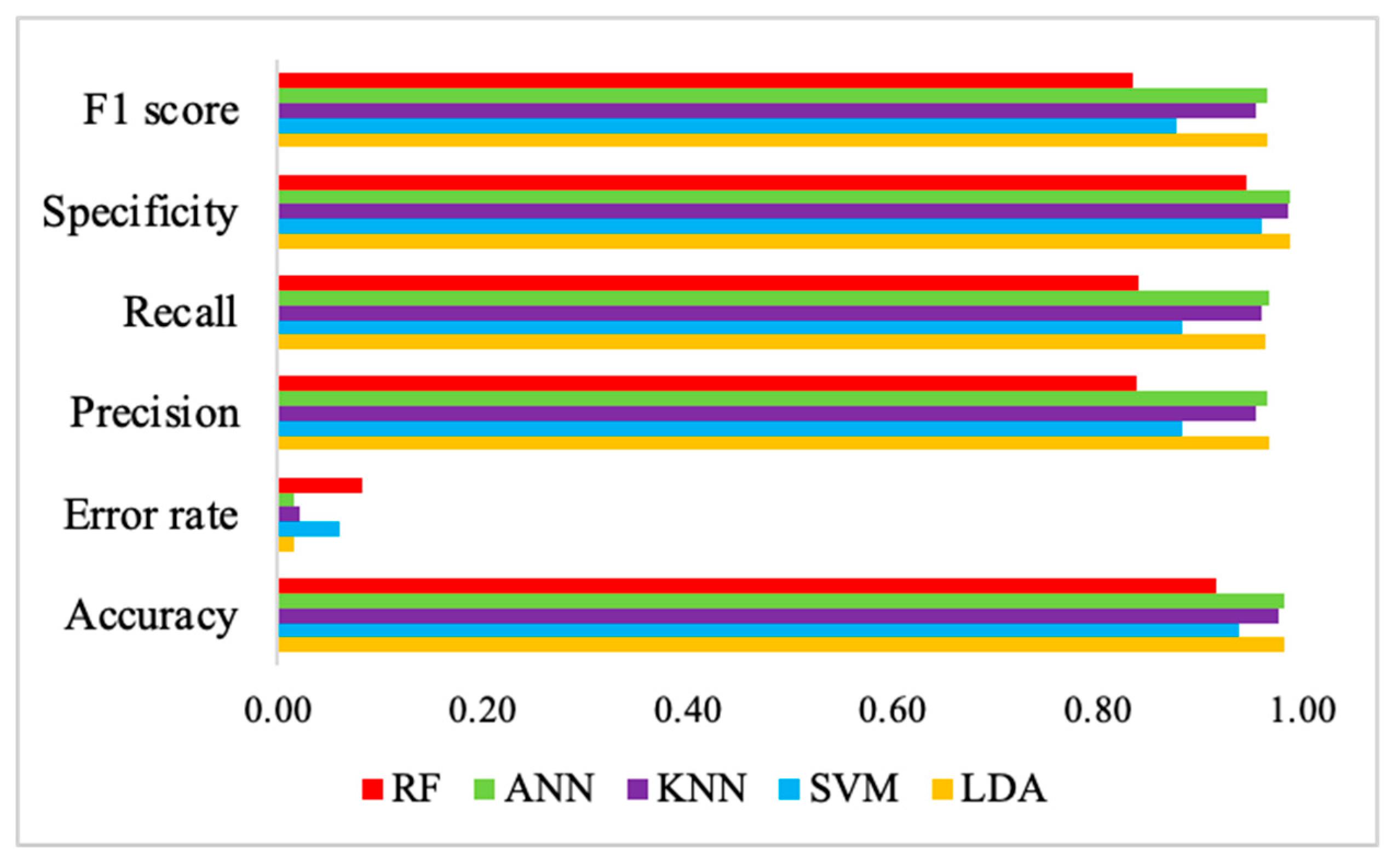
The performance of five machine learning models—LDA, SVM, KNN, ANN, and RF—was compared for classifying oolong tea samples from four geographical origins using six evaluation metrics: accuracy, error rate, precision, recall, specificity, and F1 score. In this study, for SVM, the radial basis function (RBF) kernel was used due to its effectiveness in non-linear classification tasks. The K value for KNN was set to 5 after testing values from 3 to 10, balancing accuracy and overfitting. For ANN, a three-layer feed-forward architecture with a hidden layer consisting of 10 values was selected based on preliminary trials for stable performance. RF was implemented with 100 trees. The evaluation results on the testing set are summarized in Table 4, with statistical values computed using Equations (1)–(6) and their mean values determined. Figure 5 presents the average comparison of evaluation metrics across different models. Among the tested models as presented in Table 4, LDA and ANN demonstrated the highest overall performance, both achieving 98.33% accuracy and the lowest error rate (1.67%). LDA reached 96.83% precision, 96.50% recall, 98.87% specificity, and a 96.64% F1 score, while ANN recorded 96.56% precision, 96.75% recall, 98.90% specificity, and a 96.63% F1 score. KNN also performed relatively well, with 97.78% accuracy, 2.22% error rate, 95.45% precision, 96% recall, 98.57% specificity, and a 95.54% F1 score. In contrast, SVM and RF showed lower performance, with accuracies of 93.91% and 91.67%, higher error rates (6.09% and 8.33%), and lower precision, recall, specificity, and F1 scores.
In Table 4, when assessed by tea origin, ANN delivered the best classification performance for Taiwanese oolong tea, achieving the highest accuracy (98.89%), perfect recall (100%), high precision (95.24%), and high specificity (98.57%). LDA also performed strongly with 97.78% accuracy, 95% precision, and 95% recall, while KNN achieved the same accuracy with perfect recall (100%) but slightly lower precision (90.91%). SVM and RF showed lower performance, with accuracies of 95.56% and 91.11%, respectively. For Vietnamese oolong tea, ANN and LDA performed well, achieving 98.89% and 96.67% accuracy, respectively; ANN had 100% precision and 96% recall, while LDA had 92.31% precision and 96% recall. KNN reached 97.78% accuracy with 100% precision but slightly lower recall (92%). SVM and RF were less effective, with RF showing the lowest recall (80%) despite perfect precision. Chinese oolong tea was best classified by LDA, which achieved 100% accuracy, precision, and recall, clearly separating Chinese tea samples from the others. ANN and KNN also performed well for China, both with 97.78% accuracy and 100% precision, though their recall was slightly lower (96% and 92%, respectively). For Indonesian oolong tea, LDA (98.89% accuracy) and ANN (97.78% accuracy) again showed strong performance, each achieving 95% recall, with LDA at 100% precision and ANN at 95%. KNN matched their accuracy with perfect recall (100%) but slightly lower precision (90.91%). SVM and RF showed weaker performance across all metrics for Indonesia. Overall, these findings demonstrate that a combination of an E-nose with ANN provides an effective and reliable approach for oolong tea origin classification, particularly for authenticating Taiwanese oolong tea and discriminating it from teas of other origins. Therefore, the E-nose is helpful in assessing the oolong tea quality and detecting potential fraud by analyzing aroma patterns. This makes it a useful tool for maintaining authenticity and ensuring that consumers receive genuine, high-quality oolong tea.

3.5. Gray Relational Analysis

The geographical tea origins (Taiwan, Vietnam, China, and Indonesia) were reference sequences, while the E-nose sensors (S1–S14) were comparison sequences. The normalized data, computed using Equation (7), were converted into sequence deviation, followed by the calculation of GRC values using Equations (8) and (9). The GRG values of each sensor were then obtained by averaging the corresponding GRC values using Equation (10). A higher GRG indicates closer values [29].
The average GRG values for E-nose sensors corresponding to different geographical tea origins are shown in Table 5. Among them, oolong tea from Taiwan exhibited the highest GRG values, ranging from 0.497 to 0.570, with dominant sensors S4 (ethanol, iso-butane/propane, methane, hydrogen), and S14 (ozone, iso-butane, carbon monoxide, hydrogen, ethyl alcohol, NO/NO2). In comparison, oolong tea from Vietnam had GRG values between 0.497 and 0.540, with S3 (hydrogen, methyl mercaptan, ethanol, trimethyl amine, hydrogen sulfide), S8 (ethanol, hydrogen, carbon monoxide, hydrogen sulfide), and S12 (methane, iso-butane, hydrogen, ethanol, carbon monoxide) as key sensors, while oolong tea from China showed GRG values between 0.497 and 0.530, with dominant sensors S1 (carbon monoxide, ethanol, methane, hydrogen, iso-butane), S5 (iso-butane, ethanol, hydrogen, methane), and S11 (iso-butane, hydrogen, ethanol). Oolong tea from Indonesia displayed the lowest GRG range (0.497–0.520), with S2 (ammonia, hydrogen sulfide, toluene, hydrogen, ethanol), S7 (iso-butane, hydrogen, ethanol, methane, carbon monoxide), and S10 (methane, iso-butane, hydrogen, ethanol, carbon monoxide) as the most responsive sensors. These results indicate that oolong tea from Taiwan exhibited a distinct volatile profile, as reflected by the high GRG values and the unique set of dominant sensors (S4, S6, and S14). This characteristic sensor response pattern enabled effective discrimination of Taiwanese oolong tea from teas of other origins. Overall, the different sensors responded significantly to specific geographical origins of tea, highlighting potential markers for origin-based discrimination.

4. Conclusions

In this study, machine learning models were developed for the geographical classification of oolong teas using an E-nose. MANOVA revealed statistically significant multivariate effects in color parameters (L*, a*, and b*) among the tea origins. PCA, as an unsupervised method, was ineffective for classification due to the overlap between samples. Among the tested machine learning models, ANN and LDA achieved the highest overall classification accuracy (98.33%) in classifying oolong tea samples. For specific discrimination of Taiwanese oolong tea, ANN provided the best performance, achieving the highest accuracy (98.89%). Additionally, GRA identified distinct dominant sensor responses, particularly from S4, S6, and S14, for oolong tea from Taiwan, enabling discrimination from other origins. These findings demonstrate that an E-nose combined with machine learning could be used as an effective, rapid, and non-destructive detection method for classifying oolong tea by different geographical origins. This approach provides a reliable solution for Taiwan’s tea industry to prevent fraud, protect the brand value, and meet growing consumer demand for authentic Taiwanese oolong tea. A key limitation of this study is the use of tea samples obtained from a single supplier in Taiwan. While this ensured consistency in sourcing and minimized inter-supplier variability, it may have introduced potential bias related to post-harvest handling, storage conditions, and batch-specific effects. For example, drying techniques, storage temperature and humidity, and packaging methods can significantly influence the chemical stability, bioactive compounds, sensory properties, and overall quality of tea, which may impact the reproducibility of the findings. Therefore, future studies should include samples from multiple suppliers and diverse geographical origins to further strengthen the robustness and applicability of the proposed classification model.

Supplementary Materials

The following supporting information can be downloaded at: https://www.mdpi.com/article/10.3390/chemosensors13080295/s1, Figure S1: The E-nose sensor response curve representing the three gas measurement phases.

Author Contributions

Conceptualization, S.K. and H.-H.C.; methodology, S.K. and H.-H.C.; software, S.K. and C.-C.C.; validation, H.-H.C.; formal analysis, S.K.; investigation, S.K.; resources, H.-H.C.; writing—original draft preparation, S.K.; writing—review and editing, P.R. and H.-H.C.; visualization, P.R.; supervision, H.-H.C. All authors have read and agreed to the published version of the manuscript.

Funding

This research received no external funding.

Institutional Review Board Statement

Not applicable.

Informed Consent Statement

Not applicable.

Data Availability Statement

Data are within the article.

Acknowledgments

Sushant Kaushal is grateful to the Ministry of Education (MOE), Taiwan, for the full scholarship. Also, the authors thank the Department of Food Science, National Pingtung University of Science and Technology, Pingtung, Taiwan, for providing high-end research facilities.

Conflicts of Interest

The authors declare no conflicts of interest.

References

  1. Gharibzahedi, S.M.T.; Barba, F.J.; Zhou, J.; Wang, M.; Altintas, Z. Electronic sensor technologies in monitoring quality of tea: A review. Biosensors 2022, 12, 356. [Google Scholar] [CrossRef]
  2. Hidayat, S.N.; Triyana, K.; Fauzan, I.; Julian, T.; Lelono, D.; Yusuf, Y.; Ngadiman, N.; Veloso, A.C.; Peres, A.M. The electronic nose coupled with chemometric tools for discriminating the quality of black tea samples in situ. Chemosensors 2019, 7, 29. [Google Scholar] [CrossRef]
  3. Kaushal, S.; Nayi, P.; Rahadian, D.; Chen, H.-H. Applications of electronic nose coupled with statistical and intelligent pattern recognition techniques for monitoring tea quality: A review. Agriculture 2022, 12, 1359. [Google Scholar] [CrossRef]
  4. Kombo, K.O.; Ihsan, N.; Syahputra, T.S.; Hidayat, S.N.; Puspita, M.; Wahyono; Roto, R.; Triyana, K. Enhancing classification rate of electronic nose system and piecewise feature extraction method to classify black tea with superior quality. Sci. Afr. 2024, 24, e02153. [Google Scholar] [CrossRef]
  5. Zeng, L.; Zhou, X.; Su, X.; Yang, Z. Chinese oolong tea: An aromatic beverage produced under multiple stresses. Trends Food Sci. Technol. 2020, 106, 242–253. [Google Scholar] [CrossRef]
  6. Chen, P.; Cai, J.; Zheng, P.; Yuan, Y.; Tsewang, W.; Chen, Y.; Xiao, X.; Liao, J.; Sun, B.; Liu, S. Quantitatively unravelling the impact of high altitude on oolong tea flavor from Camellia sinensis grown on the plateaus of Tibet. Horticulturae 2022, 8, 539. [Google Scholar] [CrossRef]
  7. Wang, Z.; Gan, S.; Sun, W.; Chen, Z. Quality characteristics of oolong tea products in different regions and the contribution of thirteen phytochemical components to its taste. Horticulturae 2022, 8, 278. [Google Scholar] [CrossRef]
  8. Wu, T.-H.; Tung, I.-C.; Hsu, H.-C.; Kuo, C.-C.; Chang, J.-H.; Chen, S.; Tsai, C.-Y.; Chuang, Y.-K. Quantitative analysis and discrimination of partially fermented teas from different origins using visible/near-infrared spectroscopy coupled with chemometrics. Sensors 2020, 20, 5451. [Google Scholar] [CrossRef]
  9. He, C.; Zhou, J.; Li, Y.; Ntezimana, B.; Zhu, J.; Wang, X.; Xu, W.; Wen, X.; Chen, Y.; Yu, Z. The aroma characteristics of oolong tea are jointly determined by processing mode and tea cultivars. Food Chem. X 2023, 18, 100730. [Google Scholar] [CrossRef]
  10. Su, T.-C.; Yang, M.-J.; Huang, H.-H.; Kuo, C.-C.; Chen, L.-Y. Using sensory wheels to characterize consumers’ perception for authentication of Taiwan specialty teas. Foods 2021, 10, 836. [Google Scholar] [CrossRef] [PubMed]
  11. Liu, T.-L.; Dai, J.-R.; Su, T.-C.; Chiu, C.-H.; Tsai, H.-T.; Chiu, C.-F.; Lin, J.-C.; Hu, C.-Y. Development and industrial application of geographical origin identification for Taiwanese oolong tea. J. Food Drug Anal. 2024, 32, 498. [Google Scholar] [CrossRef] [PubMed]
  12. Chiu, Y.-W. Environmental implications of Taiwanese oolong tea and the opportunities of impact reduction. Sustainability 2019, 11, 6042. [Google Scholar] [CrossRef]
  13. Lee, S.W.; Kim, B.H.; Seo, Y.H. Olfactory system-inspired electronic nose system using numerous low-cost homogenous and hetrogenous sensors. PLoS ONE 2023, 18, e0295703. [Google Scholar] [CrossRef]
  14. Jiménez-López, I.; Molina-Quiroga, J.; Gutiérrez, J.M. Classification of teas using different feature extraction methods from signals of a lab-made electronic nose. Eng. Proc. 2023, 48, 20. [Google Scholar]
  15. Gómez, I.; Lavega González, R.; Tejedor-Calvo, E.; Pérez Clavijo, M.; Carrasco, J. Odor profile of four cultivated and freeze-dried edible mushrooms by using sensory panel, electronic nose and GC-MS. J. Fungi 2022, 8, 953. [Google Scholar] [CrossRef]
  16. Putri, L.A.; Rahman, I.; Puspita, M.; Hidayat, S.N.; Dharmawan, A.B.; Rianjanu, A.; Wibirama, S.; Roto, R.; Triyana, K.; Wasisto, H.S. Rapid analysis of meat floss origin using a supervised machine learning-based electronic nose towards food authentication. npj Sci. Food 2023, 7, 31. [Google Scholar] [CrossRef]
  17. Carrillo, J.K.; Durán, C.M.; Cáceres, J.M.; Cuastumal, C.A.; Ferreira, J.; Ramos, J.; Bahder, B.; Oates, M.; Ruiz, A. Assessment of E-senses performance through machine learning models for Colombian herbal teas classification. Chemosensors 2023, 11, 354. [Google Scholar] [CrossRef]
  18. Xu, M.; Wang, J.; Zhu, L. Tea quality evaluation by applying E-nose combined with chemometrics methods. J. Food Sci. Technol. 2021, 58, 1549–1561. [Google Scholar] [CrossRef]
  19. Liu, H.; Li, Q.; Gu, Y. Convenient and accurate method for the identification of Chinese teas by an electronic nose. Qual. Assur. Saf. Crop. Foods 2018, 11, 79–88. [Google Scholar] [CrossRef]
  20. Ogundile, O.M.; Owoade, A.A.; Ogundile, O.O.; Babalola, O.P. Linear discriminant analysis based hidden Markov model for detection of Mysticetes’ vocalisations. Sci. Afr. 2024, 24, e02128. [Google Scholar] [CrossRef]
  21. Zhang, Y.; Deng, L.; Zhu, H.; Wang, W.; Ren, Z.; Zhou, Q.; Lu, S.; Sun, S.; Zhu, Z.; Gorriz, J.M.; et al. Deep learning in food category recognition. Inf. Fusion 2023, 98, 101859. [Google Scholar] [CrossRef]
  22. Liu, H.; Li, Q.; Yan, B.; Zhang, L.; Gu, Y. Bionic electronic nose based on MOS sensors array and machine learning algorithms used for wine properties detection. Sensors 2019, 19, 45. [Google Scholar] [CrossRef]
  23. Tan, J.; Xu, J. Applications of electronic nose (e-nose) and electronic tongue (e-tongue) in food quality-related properties determination: A review. Artif. Intell. Agric. 2020, 4, 104–115. [Google Scholar] [CrossRef]
  24. Stangierski, J.; Weiss, D.; Kaczmarek, A. Multiple regression models and artificial neural network (ANN) as prediction tools of changes in overall quality during the storage of spreadable processed Gouda cheese. Eur. Food Res. Technol. 2019, 245, 2539–2547. [Google Scholar] [CrossRef]
  25. Chen, G.; Zhang, X.; Wu, Z.; Su, J.; Cai, G. An efficient tea quality classification algorithm based on near infrared spectroscopy and random Forest. J. Food Process Eng. 2021, 44, e13604. [Google Scholar] [CrossRef]
  26. Huang, C.; Gu, Y. A machine learning method for the quantitative detection of adulterated meat using a MOS-based E-nose. Foods 2022, 11, 602. [Google Scholar] [CrossRef] [PubMed]
  27. Yu, D.; Gu, Y. A machine learning method for the fine-grained classification of green tea with geographical indication using a MOS-based electronic nose. Foods 2021, 10, 795. [Google Scholar] [CrossRef]
  28. Deng, J.L. Introduction to grey system theory. J. Grey Syst. 1989, 1, 1–24. [Google Scholar]
  29. Du, Z.; Hu, Y.; Buttar, N.A. Analysis of mechanical properties for tea stem using grey relational analysis coupled with multiple linear regression. Sci. Hortic. 2020, 260, 108886. [Google Scholar] [CrossRef]
  30. Du, Z.; Zhang, L.; Xie, X.; Li, D.; Li, X.; Zhang, Z.; Pang, J. Application of grey relational analysis and multiple linear regression to establish the cutting force model of oil peony stalk. Math. Probl. Eng. 2022, 2022, 2341766. [Google Scholar] [CrossRef]
  31. Chung, P.-L.; Liaw, E.-T.; Gavahian, M.; Chen, H.-H. Development and optimization of Djulis sourdough bread using taguchi grey relational analysis. Foods 2020, 9, 1149. [Google Scholar] [CrossRef] [PubMed]
  32. Rana, P.; Liaw, S.-Y.; Lee, M.-S.; Sheu, S.-C. Discrimination of four Cinnamomum species with physico-functional properties and chemometric techniques: Application of PCA and MDA models. Foods 2021, 10, 2871. [Google Scholar] [CrossRef] [PubMed]
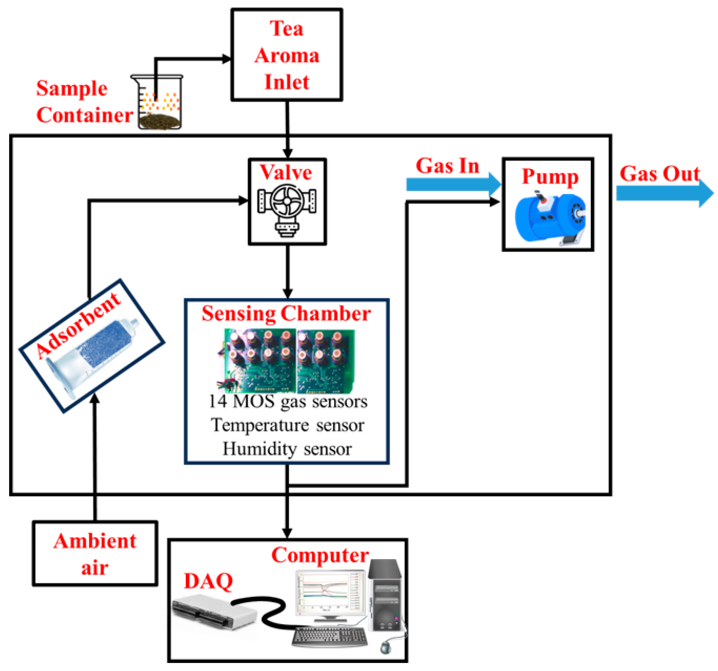
Figure 1. Schematic representation of E-nose.
Chemosensors 13 00295 g001
Figure 2. Typical response of E-nose sensor array of oolong tea samples from the four origins: (a) Taiwan; (b) Vietnam; (c) China; (d) Indonesia (1 = On Second Waiting Initial, 2 = On Round Waiting Initial, 3 = On Baseline Stable, 4 = On Collecting, 5 = On Stable).
Chemosensors 13 00295 g002
Figure 3. Radar chart of the average E-nose sensor response values for oolong tea samples from four geographical origins.
Chemosensors 13 00295 g003
Figure 4. PCA of E-nose data for oolong tea samples from four geographical origins: (a) 3-D PCA score plot showing the classification of tea samples; (b) loading plot illustrating the contributions of different sensors (S1–S14) to the first three principal components, highlighting the key variables influencing tea classification.
Chemosensors 13 00295 g004
Figure 5. Average results for comparing evaluation metrics of different models for classifying different oolong tea.
Chemosensors 13 00295 g005
Table 1. Details of response characteristics of gas sensors used in the E-nose.
Sensor No.Gas SensorTarget ApplicationTarget Gas
S1TGS-2600Air ContaminantsCarbon Monoxide, Ethanol, Methane, Hydrogen, Iso-butane
S2TGS-2602Air ContaminantsAmmonia, Hydrogen Sulfide, Toluene, Hydrogen, Ethanol
S3TGS-2603Odor and Air ContaminantsHydrogen, Methyl Mercaptan, Ethanol, Trimethyl Amine, Hydrogen Sulfide
S4TGS-2610Liquefied Petroleum (LP) GasEthanol, Iso-butane/Propane, Methane, Hydrogen
S5TGS-2611MethaneIso-butane, Ethanol, Hydrogen, Methane
S6TGS-2612Methane and LP GasMethane, Iso-Butane, Propane, Ethanol
S7TGS-2620Solvent VaporsIso-butane, Hydrogen, Ethanol, Methane, Carbon Monoxide
S8SB-51-00Hydrogen Sulfide (H2S)Ethanol, Hydrogen, Carbon Monoxide, Hydrogen Sulfide
S9SB-53-00AmmoniaEthanol, Hydrogen, Carbon Monoxide, Iso-butane, Hydrogen Sulfide, Ethylene, Methyl Mercaptan, Ammonia, Trimethylamine
S10SB-AQI-06VOCsMethane, Iso-butane, Hydrogen, Ethanol, Carbon Monoxide
S11SB-30-04AlcoholIso-butane, Hydrogen, Ethanol
S12SP3S-AQ2VOCsMethane, Iso-butane, Hydrogen, Ethanol, Carbon Monoxide
S13SP-53B-00AmmoniaEthanol, Hydrogen, Carbon Monoxide, Methane, Iso-butane, Ammonia, Nitrogen Monoxide, Nitrogen Dioxide
S14SP3-61-00OzoneOzone, Iso-butane, Carbon Monoxide, Hydrogen, Ethyl Alcohol, Nitric Oxide/Nitrogen Dioxide (NO/NO2)
Table 2. Descriptive statistics of color parameters for oolong tea samples from four geographical origins.
OriginColor Characteristics
L*a*b*
MeanSDMinMaxMeanSDMinMaxMeanSDMinMax
Taiwan19.86 c0.8718.1622.501.24 b0.370.682.099.47 c0.878.0811.29
Vietnam22.18 b1.8617.0525.702.08 a0.500.783.1611.94 b2.496.0415.15
China26.91 a4.1316.4733.520.52 c0.290.011.8811.43 b2.070.5914.89
Indonesia22.35 b3.5614.1027.061.99 a0.421.073.2213.43 a2.228.2816.53
Values are expressed as mean (n = 72), standard deviation (SD), minimum (Min), and maximum (Max). Within each column, means followed by different superscripts (a–c) are significantly different (p < 0.05) based on Duncan’s test (one-way MANOVA). Here, n = 72 represents the total number of replicate measurements per tea origin for each color parameter.
Table 3. MANOVA results of color parameters for oolong tea samples from four geographical origins.
TestValueF-ValueHypothesis dfError dfp-ValuePartial η2
Pillai’s trace1.29571.86898520.0000.432
Wilks’ Λ0.107114.9829686.4650.0000.526
Hotelling’s trace4.999155.90798420.0000.625
Roy’s largest root4.333410.218 32840.0000.812
Wilks’ Λ: Wilks’ lambda; partial η2: partial eta squared.
Table 4. Performance evaluation of five machine learning models for classifying oolong tea samples from four geographical origins.
ModelsOriginEvaluation Metrics
AccuracyError RatePrecisionRecallSpecificityF1 Score
LDATaiwan0.97780.02220.95000.95000.98570.9500
Vietnam0.96670.03330.92310.96000.96920.9412
China1.00000.00001.00001.00001.00001.0000
Indonesia0.98890.01111.00000.95001.00000.9744
Average0.98330.01670.96830.96500.98870.9664
SVMTaiwan0.95560.04440.90000.90000.97140.9000
Vietnam0.95650.04350.92000.92000.97010.9200
China0.92220.07780.95000.76000.98460.8444
Indonesia0.92220.07780.76000.95000.91430.8444
Average0.93910.06090.88250.88250.96010.8772
KNNTaiwan0.97780.02220.90911.00000.97140.9524
Vietnam0.97780.02221.00000.92001.00000.9583
China0.97780.02221.00000.92001.00000.9583
Indonesia0.97780.02220.90911.00000.97140.9524
Average0.97780.02220.95450.96000.98570.9554
ANNTaiwan0.98890.01110.95241.00000.98570.9756
Vietnam0.98890.01111.00000.96001.00000.9796
China0.97780.02220.96000.96000.98460.9600
Indonesia0.97780.02220.95000.95000.98570.9500
Average0.98330.01670.96560.96750.98900.9663
RFTaiwan0.91110.08890.77270.85000.92860.8095
Vietnam0.94440.05561.00000.80001.00000.8889
China0.87780.12220.79170.76000.92310.7755
Indonesia0.93330.06670.79170.95000.92860.8636
Average0.91670.08330.83900.84000.94510.8344
Table 5. Gray relational grade (GRG) range values of 14 E-nose sensors identified in oolong tea samples from four geographical origins.
OriginSensors
GRC RangeGRG RangeDominant Sensors
Taiwan0.350–0.6890.497–0.570S4, S6, S14
Vietnam0.333–0.6100.497–0.540S3, S8, S12
China0.336–0.5950.497–0.530S1, S5, S11
Indonesia0.340–0.5800.497–0.520S2, S7, S10
Disclaimer/Publisher’s Note: The statements, opinions and data contained in all publications are solely those of the individual author(s) and contributor(s) and not of MDPI and/or the editor(s). MDPI and/or the editor(s) disclaim responsibility for any injury to people or property resulting from any ideas, methods, instructions or products referred to in the content.