Article

Mid-Infrared Spectroscopy with Variable Selection for the Rapid Quantification of Amylose Content in Starch

1
College of Food and Bioengineering, Zhengzhou University of Light Industry, Zhengzhou 450001, China
2
College of Electrical and Electronic Engineering, Wenzhou University, Wenzhou 325035, China
3
Zhejiang Key Laboratory of Smart Low-Voltage Apparatus and New Energy Application, Wenzhou University, Wenzhou 325035, China
*
Authors to whom correspondence should be addressed.
These authors contributed equally to this work and should be considered co-first authors.
Chemosensors 2025, 13(8), 287; https://doi.org/10.3390/chemosensors13080287
Submission received: 22 June 2025 / Revised: 14 July 2025 / Accepted: 28 July 2025 / Published: 4 August 2025
(This article belongs to the Special Issue Spectroscopic Techniques for Chemical Analysis)

Abstract

Amylose content significantly influences the technological, quality, and nutritional properties of starchy foods. This study developed a rapid, non-destructive method to quantify amylose content in starch using mid-infrared (MIR) spectroscopy combined with chemometric techniques. Manually prepared starch mixtures with varying amylose levels were scanned to obtain MIR spectra, which were preprocessed using smoothing and z-score normalization to reduce operational variability. Three variable selection methods, including bootstrap soft shrinkage (BOSS), competitive adaptive reweighted sampling (CARS), and uninformative variable elimination (UVE), were applied to select the useful spectra. A partial least square (PLS) model was then constructed to correlate selected spectral data with amylose content. The results revealed that the number and position of selected variables differed across different optimization methods, which influenced the model’s performance. It is worth noting that the optimized PLS model significantly reduced the root mean squared error of cross-validation (RMSECV) and improved prediction accuracy in 50 runs. In particular, the CARS-PLS model showed superior performance, achieving a correlation coefficient (Rp) of 0.964 and a root mean squared error of prediction (RMSEP) of 4.59, a 60% improvement over the original PLS model, which had an RMSEP of 11.56. These results highlight MIR spectroscopy’s potential, combined with optimized chemometric models, for accurate amylose quantification in food quality control.

1. Introduction

Starch, a primary storage carbohydrate in plants, is a key energy source for humans [1]. Composed of amylose and amylopectin, starch is a natural polymer, where amylose consists of linear D-glucose units connected by α-1,4-glycosidic bonds, while amylopectin features a branched structure [2,3]. These biopolymers form starch’s hierarchical structure, which governs the technological and quality attributes of starch-based products [4,5,6]. Amylose content significantly influences the structural features (crystallinity, polymorphic type, etc.) of starch or starchy foods, thus altering their functional properties and quality attributes. Nevertheless, the content, polymerization degree, and conformation of amylose can vary significantly based on the origin of the starch, hence influencing the pasting, rheological, retrogradation, and quality characteristics of starch-based products [7,8,9]. Numerous studies have demonstrated that amylose plays a key role in determining the quality attributes of related products. For example, Zhang et al. [10] showed that high-amylose starch is usually utilized to improve the texture and structure of gluten-free products like noodles and bread. Also, high-amylose starch can help to modulate the postprandial blood glucose response and be used for fried or baked foods, providing a crispy texture and low digestibility for foods [11]. Therefore, the determination of amylose levels is essential for obtaining starchy products with desired qualities.
Traditional methods for measuring amylose content, such as iodometric titration, alkali dispersion, concanavalin A precipitation, and chromatographic analysis [12,13,14,15,16,17], are often complex, time-consuming, and labor-intensive, making them unsuitable for high-throughput or non-destructive online monitoring [18]. To address these limitations, spectroscopic techniques offer rapid, non-destructive alternatives. Near-infrared spectroscopy (NIRS) technology, as a low-cost and rapid non-destructive testing method applicable across many fields [19], is widely used for internal quality inspection (e.g., detecting contaminated rice [20] and predicting chlorophyll changes in Tencha [21]). However, it may produce broader, less specific absorption bands, leading to higher prediction errors for complex analytes like amylose [22]. In contrast, mid-infrared spectroscopy (MIR) provides sharp, well-defined absorption bands, making it ideal for the structural elucidation and quantitative analysis of organic compounds [18]. MIR quantifies constituent content based on the Beer–Lambert law by measuring the intensity of characteristic absorption bands. Advances in chemometrics have expanded MIR’s applications, enabling not only routine component analysis but also specialized tasks like breeding high-amylose starch varieties and producing standard reference materials (SRMs) by ensuring consistency in molecular and functional properties.
Numerous studies have conducted MIR spectroscopy for non-destructive food analysis [23,24,25], developing models for moisture in quinoa flour [24], saffron authentication and adulteration detection [25], and the water activity and humidity in fermented sausage [23]. These models demonstrated the application of multivariate calibration, which aimed to establish quantitative relationships between spectral data and reference data [26]. Notably, MIR quantitative analysis has been reported to be more effective than NIR analysis; for example, Musingarabwi et al. [27] found MIR to be more reliable for grape analysis, while Borba et al. [28] reported lower prediction errors for vitamin C, citric acid, and sugar in oranges using MIR compared to NIR. To optimize spectral models, multivariate selection methods such as uninformative variable elimination (UVE), bootstrap soft shrinkage (BOSS), and competitive adaptive reweighted sampling (CARS) are widely employed to select informative wavelengths and enhance model performance. However, studies focusing on the application of MIR spectroscopy for measuring amylose content of starch are limited, especially for high-amylose starch or SRMs.
This study aims to develop a robust, quantitative prediction model for amylose content using MIR spectroscopy. By employing UVE, BOSS, and CARS to select key wavelengths and optimize regression models, this model aims to eliminate irrelevant spectral information and enhance predictive accuracy, while artificial mixtures of amylose and amylopectin are used to control the content variables during model development, providing preliminary validation, with the aim of providing guidance for measuring the natural starches.

2. Materials and Methods

2.1. Materials and Instruments

For this investigation, to systematically investigate the effect of amylose content (AC) as the primary variable, a series of artificially formulated model mixtures were prepared using purified amylose and amylopectin standards. Amylopectin and amylose standards were purchased from the Beijing North Weiye Metrology Technology Research Institute (Beijing, China). Potassium bromide (KBr) of spectral purity was obtained from Tianjin Guangfu Science and Technology Development Co., LTD. (Tianjin, China), which served as an essential component in preparing samples for infrared spectroscopic analysis. Spectral analysis was conducted using an infrared spectrometer, the Vertex70 model, manufactured by the Bruker Company (Bremen, Germany).

2.2. Samples Preparation and Apparent Amylose Content of Samples

Various mixtures with different amylose levels were prepared, from 0% (i.e., amylopectin standard) to 100% (i.e., amylose standard) at intervals of 3%, eventually producing a total of 35 samples for analysis. Also, the actual amylose content of mixed samples was detected according to the method presented by Wang et al. [29]. In brief, starch (100 mg) was mixed with anhydrous ethanol (1.0 mL) and a NaOH solution (9 mL, 1 mol/L). The mixture was shaken continuously and then heated in boiling water for 10 min. After cooling to room temperature (25 °C), the solution was transferred to a 100 mL volumetric flask and distilled water was added. Then, 2.5 mL of the solution was mixed with 0.5 mL of acetic acid (1 mol/L), 1 mL of I2 (0.0025 mol/L)/KI (0.0065 mol/L) solution, and 46 mL of distilled water. The mixed solution was kept at room temperature for 20 min and the absorbance was measured at 620 nm. A standard curve was created to calculate the apparent amylose content of each sample.

2.3. Spectral Collection

Spectra of samples were recorded on a FT-IR spectrometer (Spectrum 100, Perkin Elmer, Inc., Waltham, MA, USA) equipped with a deuterated triglycine sulfate (DTGS) detector using an attenuated total reflectance (ATR) accessory. Each spectrum comprised 1866 discrete points, collected at 4 cm−1 resolution over 64 scans across the spectral range of 4000–400 cm−1 and recorded using an empty cell as the background. Measurements were performed in triplicate for each sample, and the average spectrum was used for analysis to ensure reproducibility. All spectra were baseline-corrected and normalized. For the calibration set, a total of 69 samples were selected (with 1 excluded as an outlier), while the remaining 35 qualified samples were used for external validation.

2.4. Spectral Pretreatments

Given the variability in spectral absorption and the difference in sample composition and manual operation, a series of spectral pretreatments were employed to reduce these variations and improve the consistency of spectral data. These spectral pretreatments were as follows: a smooth filter to reduce high-frequency noise, the deduction of mean intensity to correct for baseline offsets, normalization using the z-score to standardize the spectra, and first differential computation to eliminate the effect of light scattering and baseline drift.

2.5. Multivariate Data Statistics

2.5.1. Modeling Method

A partial least square (PLS) model was used to develop a quantitative model that connected spectral responses with the amylose content. The spectral wavelengths selected for this model were those identified as part of the “optimal portfolio” following the application of filtering screening methods. These selected spectra were then mapped onto an orthogonal linear space, where the top several latent variables (LVs) accumulated useful spectral information. The optimal number of LVs was determined based on the lowest root mean square error of cross-validation (RMSECV) during the calibration stage [30].

2.5.2. Principal Component Analysis (PCA)

PCA can simplify the complexity of large datasets by reducing their dimensionality, making it an ideal tool for visualizing sample distributions. PCA achieves this by identifying patterns and structures in data and representing them in a new and lower-dimensional space. PCA compresses data by transforming the original variables into a smaller set of uncorrelated variables, known as principal components (PCs), while maximizing the variance captured from the original data. These components are ordered by the number of variances explained in the data. By plotting the samples in the space of the first two or three PCs, one can visualize the distribution and identify patterns or clusters. This visual representation aids in understanding the patterns and relationships within the data [31]. In this work, PCA was mainly used for reducing dimensionality and visualization of sample distributions.

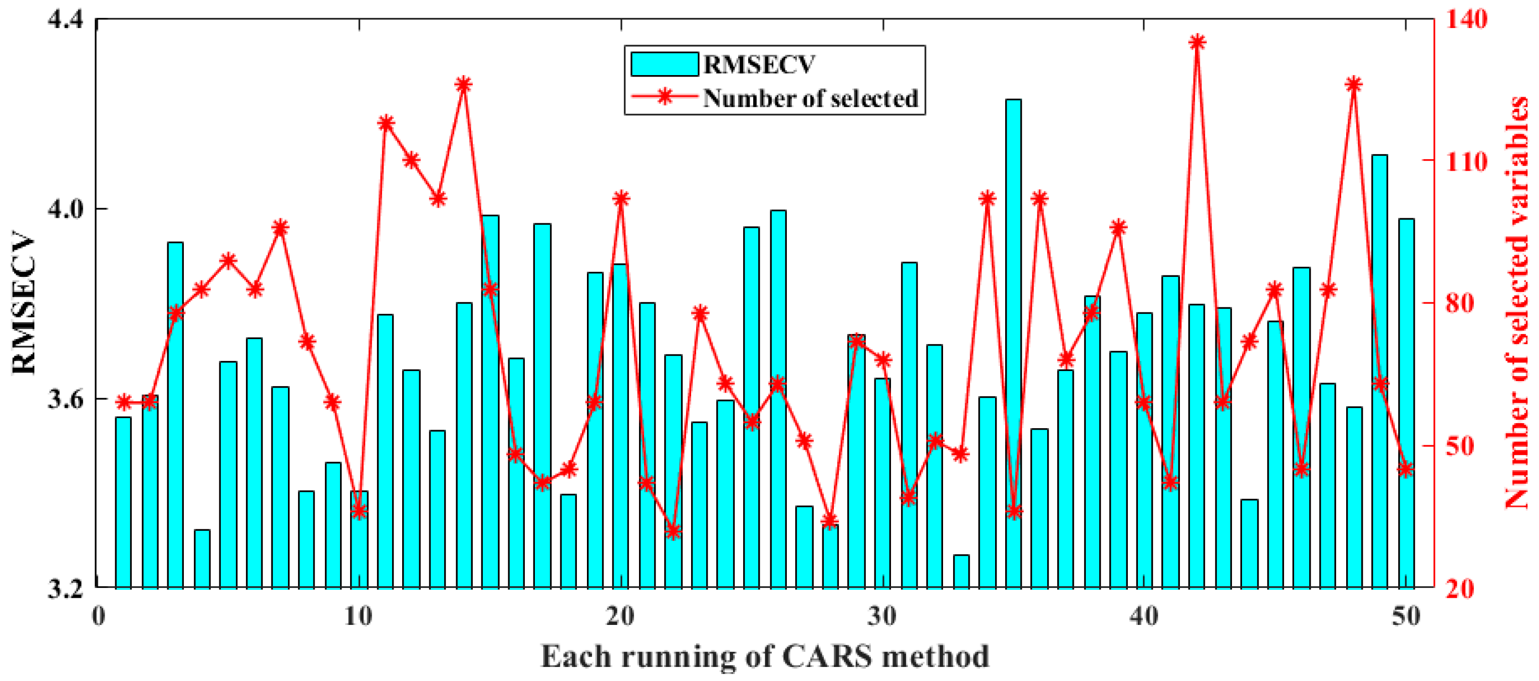
2.5.3. Competitive Adaptive Reweighted Sampling (CARS)

CARS was proposed by Li et al. [32], who revolutionized the field of spectral variable selection by introducing a dynamic and competitive strategy. It begins by setting a Monte Carlo sampling count, which determines the number of iterations for generating variable subsets or variables. Under each iteration, CARS engages in a competitive process to create N subsets of variables, each vying to contribute to the model’s predictive accuracy. It also employs an Exponential Decay Function (EDF) to systematically reduce the influence of variables with smaller regression coefficients. The EDF functions as a mathematical filter, which exponentially reduces the weights of less significant variables, thereby facilitating their eventual elimination from the model. At its core, CARS is designed to retain variables with larger absolute values of regression coefficients in the PLS model through adaptive reweighting process. Variables that fail to meet the criteria for significance are discarded, while those that contribute substantially to the model’s predictive power are retained. Its effectiveness can be attributed to its ability to identify and retain the most informative spectral variables, thus resulting in the construction of a cross-validation model optimized for minimum RMSECV.

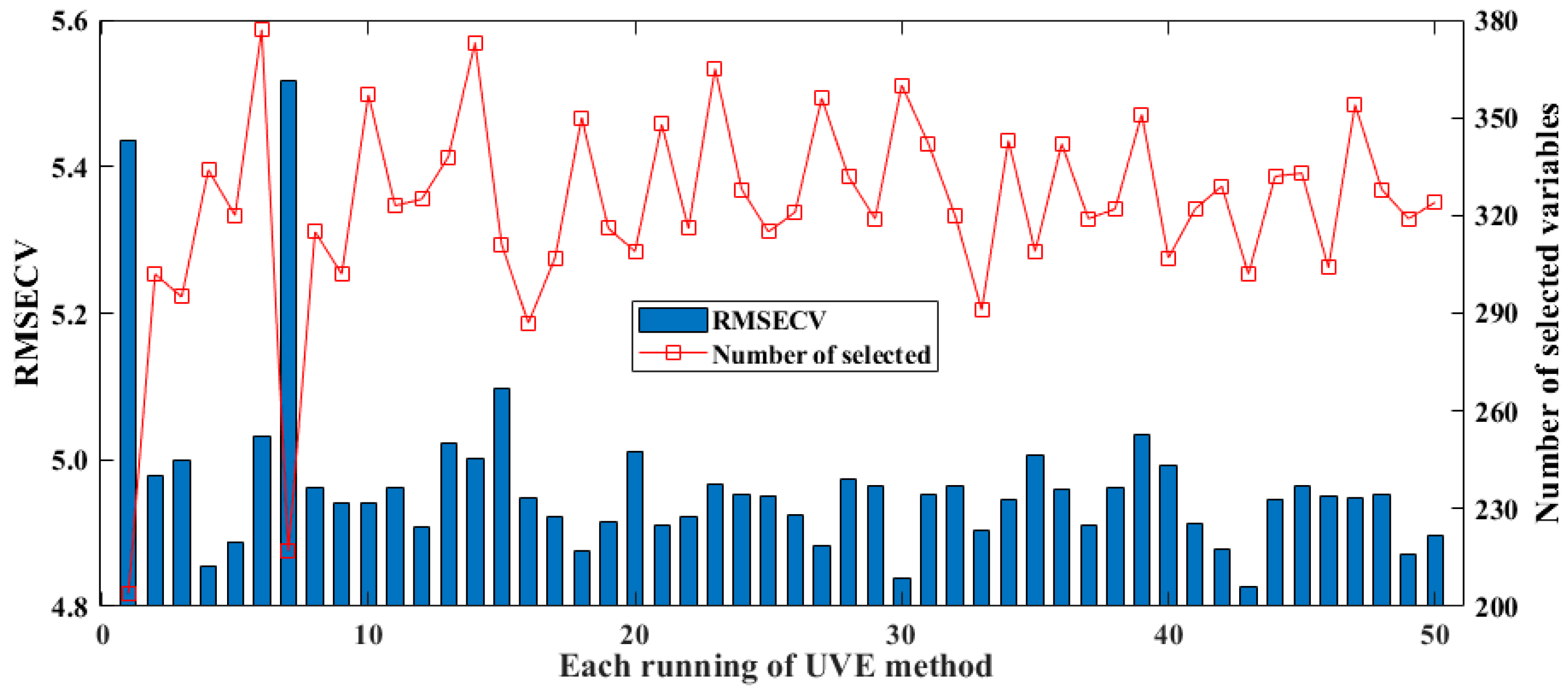
2.5.4. Uninformative Variable Elimination (UVE)

UVE focuses on identifying and removing variables that contribute little to the predictive accuracy of a model. UVE evaluates the stability of variable regression coefficients to select useful variables. If a variable’s stable regression coefficient value falls below a predefined threshold, it is discarded, while those above the threshold are retained [33]. By narrowing down the dataset to the most informative variables, UVE enhances the model’s performance and simplifies its structure. This technique is particularly valuable in handling large spectral datasets, where it can improve the efficiency and effectiveness of predictive models without sacrificing accuracy [34]. It contains several key steps like assessing variable impact, sequential elimination, and iterative modeling. UVE is widely utilized in fields such as chemometrics, environmental science, and bio-medical research, representing a robust tool for spectral data analysis and model development.

2.5.5. Bootstrapping Soft Shrinkage (BOSS)

BOSS was introduced by Deng et al. [35] as an innovative approach for assessing variable importance through the utilization of regression coefficients. It involves the following steps: (1) Bootstrap Sampling: Creating multiple subsets of variables from the original dataset; (2) Model Building: Developing a Partial Least Squares Regression (PLSR) model for each subset and assessing it with RMSECV to evaluate the model’s performance; (3) Optimal Model Selection: Choosing the model with the lowest RMSECV as the optimal one, indicating the best predictive balance; (4) Coefficient Analysis: Normalizing and summing the absolute values of the regression coefficients from all models to produce variable weights, signifying their contribution to the predictive ability; (5) Weighted Resampling: Emphasizing important variables in new subsets and rebuilding the PLSR models; (6) Iterative Process: Repeating the weighted resampling and modeling to refine variable selection; and (7) Final Selection: Selecting the subset with the smallest RMSECV as the optimal variable set. BOSS can effectively streamline the variable selection process, ensuring a robust and efficient model with minimal complexity.

2.6. Model’s Evaluation

The performance of model was assessed using several statistical metrics: the correlation coefficient (Rcv, Rp), which indicated the linear relationship between the dependent variable and dependent variables; the root mean square error of cross-validation (RMSECV) and prediction (RMSEP), which evaluated the standard deviation of residuals from the predicted results; and the mean absolute error (MAE), which represented the average magnitude of errors in a set of predictions without considering their direction [36]. In addition, relative percent deviation (RPD) was calculated by the ratio of standard deviation to RMSEP, measuring the ability of model’s prediction. These metrics collectively provided a comprehensive assessment of the model’s predictive accuracy and reliability.

2.7. Software

All calculations and data analyses in this study were conducted using Matlab software (R2024a, MathWorks Inc., Natick, MA, USA). The PLS algorithm was implemented using the iToolbox [37]. The download links for the spectral optimization algorithms UVE, CARS, and BOSS can be found in previous studies [38,39,40].

3. Results and Discussion

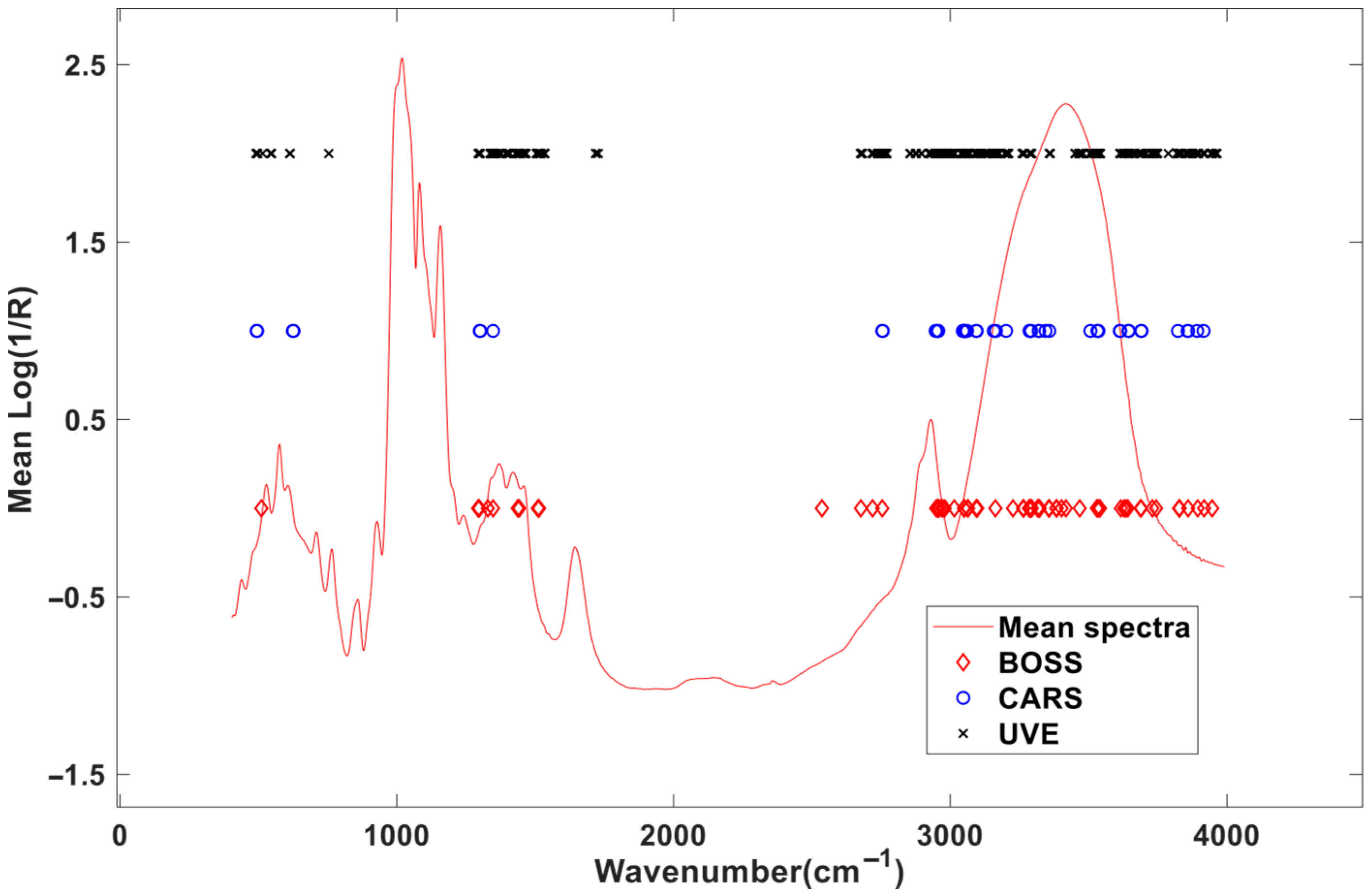
3.1. Analysis of Spectral Profile

Figure 1A displays the original spectra of the starch mixture in the range of 4000 cm−1 to 400 cm−1, where two distinct spectral peaks are clearly observed. To reduce the spectral response differences, several pretreatment methods were selected, e.g., smooth filtering, mean intensity deduction, z-score transformation, and first derivative computation. A detailed comparison of these optimized methods is provided in Section 3.3. Among these, the z-score technique exhibited the most effective optimization. Figure 1B shows the spectra after z-score pretreatment. It can be observed that the spectrum of sample No. 99, which had previously deviated from the spectral group, was brought back into alignment following pretreatment. This demonstrates the powerful effect of spectral pretreatment.

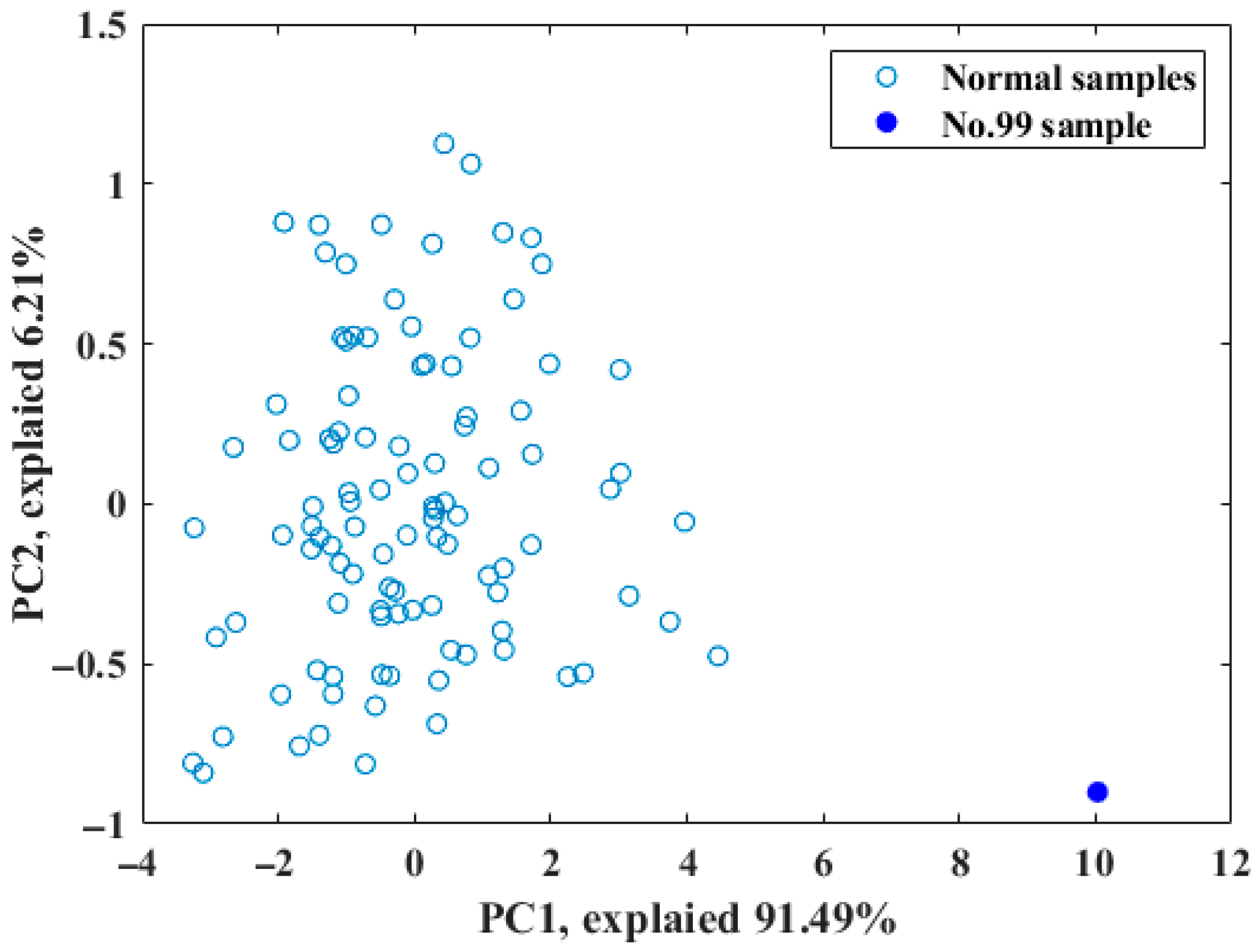
3.2. Division of Samples

In order to ensure robust model development and validation, a total of 105 starch samples were strategically divided into a calibration set and a prediction set at a ratio of 2:1. As presented in Figure 2, spectral analysis indicated that sample 99 might be an outlier due to its significant deviation from the other samples. This was further confirmed through principal component analysis (PCA), which revealed that sample 99 was distinctly separated from the cluster group in the scatter plot (Figure 2), implying that it could negatively affect the accuracy of the model and should be removed. A detailed description of the sample division is provided in Table 1, with the calibration set consisting of 69 samples and the prediction set comprising 35 samples.

3.3. Comparison of Spectra Pretreatments

In this analysis, the efficacy of four different spectral pretreatments was evaluated for their ability to increase the accuracy of PLS models. RMSECV and RMSEP were used to estimate the overall error of the developed models, where lower values indicated higher accuracy [41]. As demonstrated in Table 2, the z-score method outperformed the other methods, with an RMSECV of 9.82 and an RMSEP of 7.57, which are the lowest values among the pretreatments. This suggests that the z-score method provided the most accurate predictions in both the cross-validation and prediction phases. Furthermore, the z-score method achieved the highest correlation coefficient (Rp) of 0.971, an RPD of 3.94, and the smallest MAEp of 5.98, which surpassed the other methods, indicating a stronger linear relationship between the predicted and actual values. Additionally, the z-score method demonstrated the best correction effect on sample number 99, which had been identified as an outlier. The improvement in the bias (No. 99) value from −61.3 (without pretreatment) to −26.8 (after z-score treatment) implied that the z-score method was most effective in mitigating the influence of this outlier, thereby enhancing the overall model accuracy.
Following the comprehensive evaluation of RMSECV, RMSEP, Rcv, MAE, and the impact on the outlier sample 99, the z-score method was identified as the most effective pretreatment technique for our spectral data. Its ability to reduce the influence of outliers and minimize prediction errors made it the optimal choice for elevating the accuracy and reliability of our PLS models.

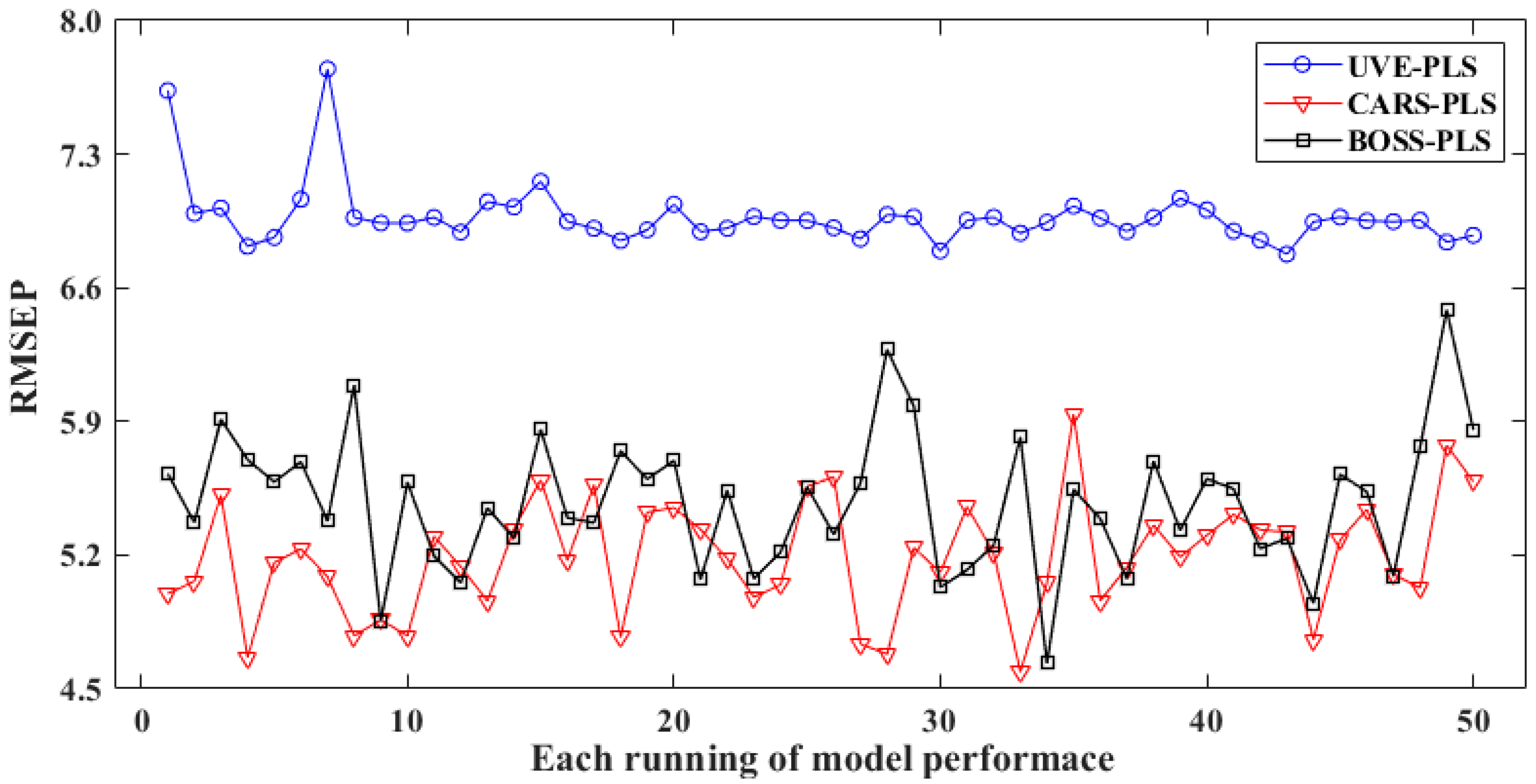
3.4. Comparison of Spectral Variables Selections

3.4.1. Optimization by BOSS

BOSS employs a strategy called soft shrinkage for variable selection. Compared to the traditional hard shrinkage strategy that directly eliminates less informative variables, soft shrinkage provides a more gradual reduction in the influence of variables. In this method, variables with less information are assigned smaller weights, but they still retain the potential for further evaluation [35]. Related results of selected spectral variables and model RMSECV obtained by BOSS over 50 runs are shown in Figure 3. The minimum, maximum, standard deviation, and average values of RMSECV for the models constructed by BOSS are 3.3003, 4.6181, 0.2553, and 3.9014, respectively. In the 34th run, BOSS obtained the lowest RMSECV, while the number of selected variables was around the mean value at about 75 variables. The performance of the developed model with more spectral screening variables in the 3rd, 17th, 32nd, and 44th runs was not significantly better than that of the model with fewer selected spectral variables. Therefore, in the BOSS screening method, the number of spectra has no significant effect on modeling performance.

3.4.2. Optimization by CARS

CARS runs N variable subsets iteratively through N sampling epochs and finally selects the subset with the lowest RMSECV value as the best subset. Figure 4 displays the results of selected spectral variables and the model’s RMSECV for CARS over 50 runs. The minimum, maximum, standard deviation, and average RMSECV values for the model constructed using CARS are 3.2677, 4.2294, 0.2146, and 3.6970, respectively. In these repeated runs, it can be found that the number of spectral variables screened varies greatly, ranging from 25 in the 22nd run to 138 in the 42nd run. It seems that it is necessary to run CARS multiple times so that a suitable optimization model can be selected.

3.4.3. Optimization by UVE

The UVE-PLS method has been widely used in earlier research [42,43]. The spectral variables selected over 50 runs and the RMSECV results of the model are shown in Figure 5. The minimum, maximum, standard deviation, and average values of the RMSECV of the model constructed by UVE are 4.8259, 5.5168, 0.1177, and 4.9656, respectively. In the 50 repeated tests, the number of spectral variables screened for modeling was higher than for the above two methods, namely BOSS and CARS. Among the test, the number of spectral variables screened in two cases was particularly low, at less than 220, while the number of variables screened in the remaining 48 tests fluctuated between 290 and 380. Therefore, in the mechanism of UVE randomly adding Gaussian noise, multiple consecutive runs must be performed to overcome the problem of insufficient model optimization caused by the randomness of this random noise.

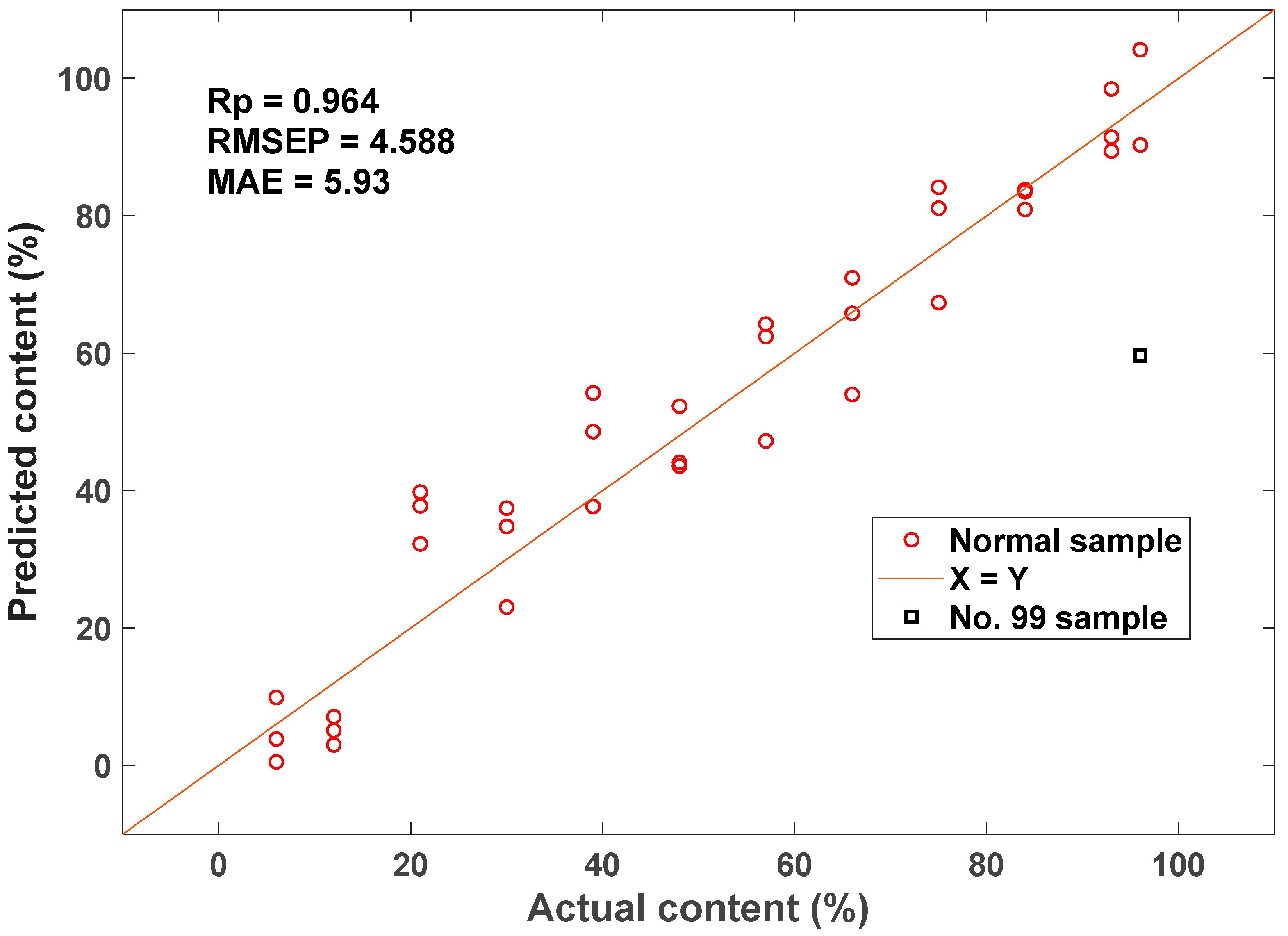
3.5. Predictions of the Optimized Regression Models

Figure 6 and Table 3 depict the optimization effects of the three variable selection methods mentioned above. Figure 6 provides a visual comparison of the RMSEP for these three methods in 50 repeated runs. It can be observed that all variable-optimized regression models performed well, and their RPD is higher than 3, indicating a strong relationship between the selected spectra and the reference. In addition, the RMSEP level of UVE-PLS is the highest, with a mean value of 6.97 and a deviation of 0.17. Among these runs, UVE obtained the best output in the fourth run, with the lowest RMSEP of 6.82, as well as a correlation coefficient (Rp) of 0.987 in the prediction set.
The RMSEP values for CARS and BOSS are 4.59 and 4.63, respectively, 32.7% and 32.1% of the corresponding value in UVE-PLS. Meanwhile, CARS and BOSS could also enhance the model by approximately 60% compared to the non-optimized version, with Rp values of 0.964 and 0.952, respectively.

3.6. Discussions

Compared with other variable selection techniques, the BOSS method offered a unique combination of computational efficiency and predictive accuracy. Generally, BOSS employs an iterative process to refine variable selection through multiple stages, including the use of kernel functions that map input data into a higher dimensional space, where linear separation is more feasible. This approach enables BOSS to effectively handle complex datasets and enhance model classification performance, particularly in spectral analysis. Furthermore, BOSS is more competitive with other methods in terms of computational efficiency, employing mathematical transformations and optimizations to reduce data dimensionality as well as retain the most informative variables. This efficient process allows for faster model training and prediction times, making it well-suited for large-scale applications.
From the distribution of the selected spectral positions in Figure 7, the variables screened by the three methods are distributed in the same area, mainly in three areas, namely 500–800 cm−1, 1300–1800 cm−1, and 2800–3900 cm−1, indicating that these areas are very important to MIR spectral modeling for amylose content in starch. Among them, the selected MIR spectral variables in the 1000–1200 cm−1 range correspond to C-O-C stretching vibrations of amylose’s glycosidic bonds; the spectral variables located around 2800–3000 cm−1 are associated with C-H stretching, which are indicative of amylose’s aliphatic backbone; and the MIR spectra located in the 3200–3400 cm−1 range are linked to O-H stretching, reflecting hydrogen bonding in amylose. These assignments provide insight into the molecular basis of the model’s predictive accuracy.
Regarding predictive accuracy, BOSS demonstrated its effectiveness through the use of regression coefficients so as to evaluate variable importance. This method systematically eliminated variables with a minimal impact on model performance, which ensured that the final model was not only accurate but also robust against over-fitting. Also, BOSS has been shown to maintain or even improve predictive accuracy compared to other variable selection approaches, demonstrating it as a valuable tool for advancing the performance of models across various fields, including chemometrics and biomedical research [44]. Normally, the performance of BOSS can be affected by the specific characteristics of the dataset and the problem being addressed, similar to other variable selection techniques. However, its iterative refinement process and the application of advanced mathematical techniques make BOSS a strong candidate for tasks where both computational efficiency and predictive accuracy are critical. NIR spectroscopy with BOSS has higher accuracy than Raman spectroscopy in terms of the quantitative analysis of corn and cassava amylose starch [45]. Xie et al. [46] classified glutinous rice flour by using NIR spectroscopy combined with a modified partial least square model to identify amylose content and amylopectin content. Obviously, the method used in this study has more advantages in quantifying amylose in the model system.

4. Conclusions

Thirty-five sets of starch samples with varying amylose/amylopectin ratios were prepared, and the spectra were collected in the frequency range of 4000–400 cm−1 through MIR spectroscopy. A comparison was performed between the results of various preprocessing techniques, including mean intensity subtraction, z-score normalization, smooth filtering, and first derivative computation. The results indicated that the z-score method yielded the best optimization. It effectively corrected deviations from the cluster’s baseline spectra. After applying z-score pretreatment, the RMSECV decreased from 10.79 to 9.82. The amylose prediction model was constructed using UVE, CARS, and BOSS combined with PLS. Compared with the other three variable selection methodologies, the results of CARS displayed the best optimization effect on the prediction model. Moreover, the RMSEP optimization of the model was more than 60% in comparison with the original model without variable selection. The distribution plot for amylose content prediction constructed using CARS-PLS is shown in Figure 8. The final results reveal that the amylose content detection model developed using MIR spectroscopy combined with chemometrics can realize the rapid detection of amylose.
While our study demonstrates the effectiveness of MIR spectroscopy, a direct experimental comparison with NIR was not conducted due to equipment limitations. Future work should include such comparisons to further validate MIR’s advantages for amylose quantification. Future studies should expand testing to include additional botanical sources, such as potato, to further validate the model’s applicability in diverse real-world scenarios

Author Contributions

Conceptualization, Y.Z. and L.Y.; Data curation, J.B., Y.L. and X.L.; Formal analysis, H.W. and Y.L.; Funding acquisition, Y.Z. and L.Y.; Investigation, J.Q., J.B. and X.L.; Methodology, Y.Z. and L.Y.; Project administration, H.W., Y.Z. and L.Y.; Resources, Y.Z.; Software, X.L. and L.Y.; Validation, J.B. and X.L.; Visualization, J.Q. and H.W.; Writing—original draft, J.Q. and H.W.; Writing—review and editing, Y.Z. and L.Y. All authors have read and agreed to the published version of the manuscript.

Funding

This research was financially supported by the Key Research and Development Project of Henan Province (231111113200), the Higher Education Science and Technology Innovation Talent Program of Henan Province (25HASTIT040), the Higher Education School Young Backbone Teacher Training Program of Henan Province (2024GGJS078), and the Natural Science Foundation of Guangdong Province (CN) (2025A1515011509).

Institutional Review Board Statement

Not applicable.

Informed Consent Statement

Not applicable.

Data Availability Statement

Data are available on request.

Conflicts of Interest

The authors declare no conflicts of interest.

References

  1. Chi, C.; Xu, K.; Wang, H.; Zhao, L.; Zhang, Y.; Chen, B.; Wang, M. Deciphering multi-scale structures and pasting properties of wheat starch in frozen dough following different freezing rates. Food Chem. 2023, 405, 134836. [Google Scholar] [CrossRef]
  2. Cheng, W.; Sun, Y.; Xia, X.; Yang, L.; Fan, M.; Li, Y.; Wang, L.; Qian, H. Effects of β-amylase treatment conditions on the gelatinization and retrogradation characteristics of wheat starch. Food Hydrocoll. 2022, 124, 107286. [Google Scholar] [CrossRef]
  3. Sun, X.; Sun, Z.; Saleh, A.S.M.; Zhao, K.; Ge, X.; Shen, H.; Zhang, Q.; Yuan, L.; Yu, X.; Li, W. Understanding the granule, growth ring, blocklets, crystalline and molecular structure of normal and waxy wheat A- and B-starch granules. Food Hydrocoll. 2021, 121, 107034. [Google Scholar] [CrossRef]
  4. Liu, X.; Zhang, J.; Yang, X.; Sun, J.; Zhang, Y.; Su, D.; Zhang, H.; Wang, H. Combined molecular and supramolecular structural insights into pasting behaviors of starches isolated from native and germinated waxy brown rice. Carbohydr. Polym. 2022, 283, 119148. [Google Scholar] [CrossRef]
  5. Wang, H.; Liu, J.; Zhang, Y.; Li, S.; Liu, X.; Zhang, Y.; Zhao, X.; Shen, H.; Xie, F.; Xu, K.; et al. Insights into the hierarchical structure and physicochemical properties of starch isolated from fermented dough. Int. J. Biol. Macromol. 2024, 267, 131315. [Google Scholar] [CrossRef]
  6. Bian, X.; Chen, J.; Yang, Y.; Yu, D.; Ma, Z.; Ren, L.; Wu, N.; Chen, F.; Liu, X.; Wang, B.; et al. Effects of fermentation on the structure and physical properties of glutinous proso millet starch. Food Hydrocoll. 2022, 123, 107144. [Google Scholar] [CrossRef]
  7. Ma, M.; Gu, Z.; Cheng, L.; Li, Z.; Li, C.; Hong, Y. Chewing characteristics of rice and reasons for differences between three rice types with different amylose contents. Int. J. Biol. Macromol. 2024, 278, 134869. [Google Scholar] [CrossRef]
  8. Waterschoot, J.; Gomand, S.V.; Fierens, E.; Delcour, J.A. Production, structure, physicochemical and functional properties of maize, cassava, wheat, potato and rice starches. Starch-Stärke 2013, 67, 14–29. [Google Scholar] [CrossRef]
  9. Leal-Lazareno, C.; Agama-Acevedo, E.; Ibba, M.I.; Ammar, K.; Bello-Pérez, L. Structural, molecular, and physicochemical properties of starch in high-amylose durum wheat lines. Food Hydrocoll. 2025, 160, 110791. [Google Scholar] [CrossRef]
  10. Zhong, Y.; Tai, L.; Blennow, A.; Ding, L.; Herburger, K.; Qu, J.; Xin, A.; Guo, D.; Hebelstrup, K.; Liu, X. High-amylose starch: Structure, functionality and applications. Crit. Rev. Food Sci. 2023, 63, 8568–8590. [Google Scholar] [CrossRef] [PubMed]
  11. Obadi, M.; Qi, Y.; Xu, B. High-amylose maize starch: Structure, properties, modifications and industrial applications. Carbohydr. Polym. 2023, 299, 120185. [Google Scholar] [CrossRef] [PubMed]
  12. Li, D.; Zhu, F. Characterization of polymer chain fractions of kiwifruit starch. Food Chem. 2018, 240, 579–587. [Google Scholar] [CrossRef] [PubMed]
  13. Creek, J.A.; Benesi, A.; Runt, J.; Ziegler, G.R. Potential sources of error in the calorimetric evaluation of amylose content of starches. Carbohydr. Polym. 2007, 68, 465–471. [Google Scholar] [CrossRef]
  14. Mariotti, M.; Fongaro, L.; Catenacci, F. Alkali spreading value and image analysis. J. Cereal Sci. 2010, 52, 227–235. [Google Scholar] [CrossRef]
  15. Zhu, F.; Cui, R. Comparison of molecular structure of oca (Oxalis tuberosa), potato, and maize starches. Food Chem. 2019, 296, 116–122. [Google Scholar] [CrossRef]
  16. Shi, P.; Zhao, Y.; Qin, F.; Liu, K.; Wang, H. Understanding the multi-scale structure and physicochemical properties of millet starch with varied amylose content. Food Chem. 2023, 410, 135422. [Google Scholar] [CrossRef]
  17. Yang, X.; Chi, C.; Liu, X.; Zhang, Y.; Zhang, H.; Wang, H. Understanding the structural and digestion changes of starch in heat-moisture treated polished rice grains with varying amylose content. Int. J. Biol. Macromol. 2019, 139, 785–792. [Google Scholar] [CrossRef]
  18. Khoomtong, A.; Noomhorm, A. Development of a simple portable amylose content meter for rapid determination of amylose content in milled rice. Food Bioprocess Technol. 2015, 8, 1938–1946. [Google Scholar] [CrossRef]
  19. Lohumi, S.; Lee, S.; Lee, H.; Cho, B.K. A review of vibrational spectroscopic techniques for the detection of food authenticity and adulteration. Trends Food Sci. Technol. 2015, 46, 85–98. [Google Scholar] [CrossRef]
  20. Song, C.; Liu, J.; Wang, C.; Li, Z.; Zhang, D.; Li, P. Rapid identification of adulterated rice based on data fusion of near-infrared spectroscopy and machine vision. J. Food Meas. Charact. 2024, 18, 3881–3892. [Google Scholar] [CrossRef]
  21. Liu, L.; Zareef, M.; Wang, Z.; Li, H.; Chen, Q.; Ouyang, Q. Monitoring chlorophyll changes during Tencha processing using portable near-infrared spectroscopy. Food Chem. 2023, 412, 135505. [Google Scholar] [CrossRef]
  22. Pasquini, C. Near infrared spectroscopy: A mature analytical technique with new perspectives–A review. Anal. Chim. Acta 2018, 1026, 8–36. [Google Scholar] [CrossRef]
  23. Collell, C.; Gou, P.; Arnau, J.; Muñoz, I.; Comaposada, J. NIR technology for on-line determination of superficial aw and moisture content during the drying process of fermented sausages. Food Chem. 2012, 135, 1750–1755. [Google Scholar] [CrossRef]
  24. González-Muñoz, A.; Montero, B.; Enrione, J.; Matiacevich, S. Rapid prediction of moisture content of quinoa (Chenopodium quinoa Willd.) flour by Fourier transform infrared (FTIR) spectroscopy. J. Cereal Sci. 2016, 71, 246–249. [Google Scholar] [CrossRef]
  25. Amirvaresi, A.; Nikounezhad, N.; Amirahmadi, M.; Daraei, B.; Parastar, H. Comparison of near-infrared (NIR) and mid-infrared (MIR) spectroscopy based on chemometrics for saffron authentication and adulteration detection. Food Chem. 2021, 344, 128647. [Google Scholar] [CrossRef]
  26. Porep, J.U.; Kammerer, D.R.; Carle, R. On-line application of near infrared (NIR) spectroscopy in food production. Trends Food Sci. Technol. 2015, 46, 211–230. [Google Scholar] [CrossRef]
  27. Yuan, L.-M.; Mao, F.; Chen, X.; Li, L.; Huang, G. Non-invasive measurements of ‘Yunhe’ pears by vis-NIRS technology coupled with deviation fusion modeling approach. Postharvest Biol. Technol. 2020, 160, 111067–111073. [Google Scholar] [CrossRef]
  28. Borba, K.R.; Spricigo, P.C.; Aykas, D.P.; Mitsuyuki, M.C.; Colnago, L.A.; Ferreira, M.D. Non-invasive quantification of vitamin C, citric acid, and sugar in ‘Valência’oranges using infrared spectroscopies. J. Food Sci. Technol. 2021, 58, 731–738. [Google Scholar] [CrossRef] [PubMed]
  29. Wang, H.; Wang, Y.; Wang, R.; Liu, X.; Zhang, Y.; Zhang, H.; Chi, C. Impact of long-term storage on multi-scale structures and physicochemical properties of starch isolated from rice grains. Food Hydrocoll. 2022, 124, 107255. [Google Scholar] [CrossRef]
  30. Yuan, L.-M.; Yang, X.; Fu, X.; Yang, J.; Chen, X.; Huang, G.; Chen, X.; Li, L.; Shi, W. Consensual Regression of Lasso-Sparse PLS models for Near-Infrared Spectra of Food. Agriculture 2022, 12, 1804. [Google Scholar] [CrossRef]
  31. Granato, D.; Santos, J.S.; Escher, G.B.; Ferreira, B.L.; Maggio, R.M. Use of principal component analysis (PCA) and hierarchical cluster analysis (HCA) for multivariate association between bioactive compounds and functional properties in foods: A critical perspective. Trends Food Sci. Technol. 2018, 72, 83–90. [Google Scholar] [CrossRef]
  32. Li, H.; Liang, Y.; Xu, Q.; Cao, D. Key wavelengths screening using competitive adaptive reweighted sampling method for multivariate calibration. Anal. Chim. Acta 2009, 648, 77–84. [Google Scholar] [CrossRef] [PubMed]
  33. Centner, V.; Massart, D.L.; de Noord, O.E.; de Jong, S.; Vandeginste, B.M.; Sterna, C. Elimination of uninformative variables for multivariate calibration. Anal. Chem. 1996, 68, 3851–3858. [Google Scholar] [CrossRef]
  34. Koshoubu, J.; Iwata, T.; Minami, S. Elimination of the uninformative calibration sample subset in the modified UVE (uninformative variable elimination)–PLS (partial least squares) method. Anal. Sci. 2001, 17, 319–322. [Google Scholar] [CrossRef]
  35. Deng, B.; Yun, Y.; Cao, D.; Yin, Y.; Wang, W.; Lu, H.; Luo, Y.; Liang, Y. A bootstrapping soft shrinkage approach for variable selection in chemical modeling. Anal. Chim. Acta 2016, 908, 63–74. [Google Scholar] [CrossRef] [PubMed]
  36. Li, M.; Lv, W.; Zhao, R.; Guo, H.; Liu, J.; Han, D. Non-destructive assessment of quality parameters in ‘Friar’plums during low temperature storage using visible/near infrared spectroscopy. Food Control 2017, 73, 1334–1341. [Google Scholar] [CrossRef]
  37. Glaucio, L.A.; Reis, A.S.; Besen, M.S.; Rodrigues, M.; Crusiol, L.; Falcioni, R.; Oliveira, R.; Batista, M.; Nanni, M. Spectral method for macro and micronutrient prediction in soybean leaves using interval partial least squares regression. Eur. J. Agron. 2023, 143, 126717. [Google Scholar] [CrossRef]
  38. Yuan, L.; Mao, F.; Huang, G.; Chen, X.; Wu, D.; Li, S.; Zhou, X.; Jiang, Q.; Lin, D.; He, R. Models fused with successive CARS-PLS for measurement of the soluble solids content of Chinese bayberry by vis-NIRS technology. Postharvest Biol. Technol. 2020, 169, 111308. [Google Scholar] [CrossRef]
  39. Gao, F.; Xing, Y.; Li, J.; Guo, L.; Sun, Y.; Shi, W.; Yuan, L. Prediction of Total Soluble Solids in Apricot Using Adaptive Boosting Ensemble Model Combined with NIR and High-Frequency UVE-Selected Variables. Molecules 2025, 30, 1543. [Google Scholar] [CrossRef]
  40. Yun, Y.-H.; Li, H.-D.; Deng, B.-C.; Cao, D.-S. An overview of variable selection methods in multivariate analysis of near-infrared spectra. TrAC Trends Anal. Chem. 2019, 113, 102–115. [Google Scholar] [CrossRef]
  41. Hearn, L.K.; Subedi, P.P. Determining levels of steviol glycosides in the leaves of Stevia rebaudiana by near infrared reflectance spectroscopy. J. Food Compos. Anal. 2009, 22, 165–168. [Google Scholar] [CrossRef]
  42. Du, G.; Cai, W.; Shao, X. A variable differential consensus method for improving the quantitative near-infrared spectroscopic analysis. Sci. China Chem. 2012, 55, 1946–1952. [Google Scholar] [CrossRef]
  43. Han, Q.; Wu, H.; Cai, C.; Xu, L.; Yu, R. An ensemble of Monte Carlo uninformative variable elimination for wavelength selection. Anal. Chim. Acta 2008, 612, 121–125. [Google Scholar] [CrossRef]
  44. Yuan, L.-M.; Liu, Y.; Gao, F.; Jiang, Q.; Ji, H.; Chen, X.; Chen, X.; Zhu, F. Prediction of bayberry SSC by ensemble model with random frog successively selected from the residual vis-NIR spectra. Food Control 2025, 178, 111525. [Google Scholar] [CrossRef]
  45. Mariana, R.A.; Laura, B.R.; Ronei, J.P. Determination of amylose content in starch using Raman spectroscopy and multivariate calibration analysis. Anal. Bioanal. Chem. 2010, 397, 2693–2701. [Google Scholar] [CrossRef]
  46. Xie, L.H.; Tang, S.Q.; Wei, X.J.; Sheng, Z.H.; Shao, G.N.; Jiao, G.A.; Hu, S.K.; Wang, L.; Hu, P.S. Simultaneous determination of apparent amylose, amylose and amylopectin content and classification of waxy rice using near-infrared spectroscopy (NIRS). J. Food Chem. 2022, 388, 132944. [Google Scholar] [CrossRef] [PubMed]
Figure 1. Plots of infrared spectra of the mixed starch samples. (A) Raw spectra of mixed starch; (B) preprocessed spectra with z-score method.
Chemosensors 13 00287 g001
Figure 2. Distribution of samples in the top two subspaces according to PCA.
Chemosensors 13 00287 g002
Figure 3. Results of selected spectral variables and the model’s RMSECV for BOSS in 50 runs.
Chemosensors 13 00287 g003
Figure 4. Results of selected spectral variables and model’s RMSECV for CARS in 50 runs.
Chemosensors 13 00287 g004
Figure 5. Results of selected spectral variables and model’s RMSECV for UVE in 50 runs.
Chemosensors 13 00287 g005
Figure 6. Predictive performance of optimized models via variable selection in 50 runs.
Chemosensors 13 00287 g006
Figure 7. Distributions of the selected variables by the optimization methods.
Chemosensors 13 00287 g007
Figure 8. Scatter plot of actual versus predicted amylose content by CARS-PLS.
Chemosensors 13 00287 g008
Table 1. Sample divisions and their statistics.
ItemsSample NumberMeanStdC.V. aAmylose Content Level b
Calibration set6950.2630.550.6080, 3, 9, 15, 18, 24, 27, 33, 36, 42, 45, 51, 54, 60, 63, 69, 72, 78, 81, 87, 90, 99, 100
Prediction set355129.820.5856, 12, 21, 30, 39, 48, 57, 66, 75, 84, 93, 96 c
Note: a: coefficient of variation; b: three samples were taken for each concentration as parallel tests; c: one sample (No. 99) at this concentration was abnormal, and its spectral data was excluded.
Table 2. Comparison of different pretreatments using the PLS method.
PretreatmentsLVsRcvRMSECVMAERpRMSEPMAERPDBias (No. 99)
None140.93710.788.250.92011.568.712.58−61.3
Smooth a140.94410.047.510.94010.257.942.91−61.6
z-score110.9459.827.640.9717.575.983.94−26.8
De-mean b130.84210.237.910.9509.597.613.11−57.6
Derivative c90.93810.588.100.88913.6610.432.18−22.4
Note: a: the spectral signal was smoothed using a moving average filter with a window width of 7; b: the mean intensity of the spectral signal was reduced; c: first derivative computation by using the Savitsky–Golay algorithm with a window width of 5 and two order polynomials; LVs: latent variables in the PLS model; Rcv: correlation coefficient of cross-validation; RMSECV: root mean squared error of cross-validation; MAE: mean absolute error.
Table 3. The optimal model prediction performance of each variable selection method.
Selection MethodInputsCalibration SetPrediction Set
NumberLVsRcvRMSECVMean ± SD aRpRMSEPMean ± SD bRPDBias (No. 99)
UVE-4th334150.9874.864.96 ± 0.120.9696.826.97 ± 0.174.37−36.6
CARS-33rd48140.9833.273.69 ± 0.210.9644.595.19 ± 0.306.49−36.4
BOSS-34th71130.9943.303.90 ± 0.250.9524.635.48 ± 0.366.44−31.5
none1860140.93710.78 0.92011.56 2.58−61.3
Note: a: the average value and its standard deviation in the calibration stage from 50 runs. b: The average value and its standard deviation in the predicting stage from 50 runs.
Disclaimer/Publisher’s Note: The statements, opinions and data contained in all publications are solely those of the individual author(s) and contributor(s) and not of MDPI and/or the editor(s). MDPI and/or the editor(s) disclaim responsibility for any injury to people or property resulting from any ideas, methods, instructions or products referred to in the content.

