Article

Carbon Futures Trading and Short-Term Price Prediction: An Analysis Using the Fractal Market Hypothesis and Evolutionary Computing

1
Dublin Energy Laboratory, Technological University Dublin, D07 EWV4 Dublin, Ireland
2
School of Electrical and Electronic Engineering, Technological University Dublin, D07 EWV4 Dublin, Ireland
3
Mace Group, 8 Dublin, Ireland
4
Centre for Advanced Studies, Warsaw University of Technology, Plac Politechniki 1, 00-661 Warsaw, Poland
5
Department of Computer Science, University of Western Cape, Robert Sobukwe Rd, Bellville, Cape Town 7535, South Africa
6
Faculty of Arts, Science and Technology, Wrexham Glyndŵr University of Wales, Mold Rd, Wrexham LL11 2AW, UK
7
School of Mathematics, Statistics and Computer Science, University of KwaZulu-Natal, University Rd, Westville, Durban 3629, South Africa
*
Author to whom correspondence should be addressed.
These authors contributed equally to this work.
Mathematics 2021, 9(9), 1005; https://doi.org/10.3390/math9091005
Submission received: 1 March 2021 / Revised: 6 April 2021 / Accepted: 24 April 2021 / Published: 29 April 2021
(This article belongs to the Special Issue Fractal Market Hypothesis, Trend Analysis and Future Price Prediction)

Abstract

:
This paper presents trend prediction results based on backtesting of the European Union Emissions Trading Scheme futures market. This is based on the Intercontinental Exchange from 2005 to 2019. An alternative trend prediction strategy is taken that is predicated on an application of the Fractal Market Hypothesis (FMH) in order to develop an indicator that is predictive of short term future behaviour. To achieve this, we consider that a change in the polarity of the Lyapunov-to-Volatility Ratio precedes an associated change in the trend of the European Union Allowances (EUAs) price signal. The application of the FMH in this case is demonstrated to provide a useful tool in order to assess the likelihood of the market becoming bear or bull dominant, thereby helping to inform carbon trading investment decisions. Under specific conditions, Evolutionary Computing methods are utilised in order to optimise specific trading execution points within a trend and improve the potential profitability of trading returns. Although the approach may well be of value for general energy commodity futures trading (and indeed the wider financial and commodity derivative markets), this paper presents the application of an investment indicator for EUA carbon futures risk modelling and investment trend analysis only.

1. Context, Background and Structure

Creating a commodity price for Greenhouse Gas (GHG) emissions is now a key policy measure for climate change mitigation globally. However, without a sufficiently strong market signal for GHG emissions reduction and the transition sustainable practices across all major sectors, it will become even more difficult (and costly) to implement the fundamental transformation which is now required to achieve the requirements of the Paris Accord (i.e., to limit global temperature rise to less than 2 °C). Consequently, due to the inaction thus far, this needs to happen on a much steeper pathway than was ever previously considered possible.

1.1. Context

Signatories to the Paris Accord have ratified the intent to use carbon commodities as the key financial incentive mechanism to limit further climate change. The extent of change now needed is such, that environmental and carbon commodity markets could yet become some of the most important traded commodities in the world. It is positive (and necessary) to see an emerging trend in recent economic and policy research, whereby the impact of failing to sufficiently reduce carbon intensity levels is being shown to prove much more costly (for nations, regions, cities, and individuals alike) than the ‘do nothing’ scenario. This is the first clear warning signal for banks, hedge funds, pensions and private investors to actively seek out investments with an ‘environmental view’, and, on such a scale as to facilitate the level of change necessary. Perhaps encouragingly, this is now becoming a more common trend in some of the larger investment fund firms as Environmental, Social and (Corporate) Governance (ESG) comes to the fore, and, perhaps more crudely, the growing fear of stranded investments in carbon intense sectors.
Delivering the rapid changes in energy investment patterns that are required to meet this target requires significant and sustained national and international policy measures. In response to this, an increasing number of countries have already implemented, or are in the process of implementing, GHG Emissions Trading Schemes (ETS). The first of these schemes to be implemented globally was the European Union Emissions Trading Scheme (EU ETS). This is still the largest ETS scheme in the world, and with further planned expansion of this scheme and the predicted growth in carbon trading elsewhere, it indicates a global market with a turnover of in the region of $2 trillion by 2030 [1]. This compares with 2018, where the market for carbon credits was worth just $144 billion [2].
The emergence of this new commodity class has created a range of new interactions across a range of energy related commodities, such as electricity generation, oil, coal, and gas. With underlying market challenges (which persisted for the better part of a decade) perhaps finally being overcome, the potential of these new markets and how they will effect traditional commodity pricing towards 2030 and 2050 climate change targets is only beginning to be understood. Therefore, there is a potential use for the development of a trading algorithm applicable to carbon trading on the EU ETS which takes account of the characteristics of the commodity class and provides a price trend signal to guide investment decision-making. Whilst there are many emissions trading schemes being implement world-wide, the EU ETS carbon market is the largest and most advanced. As a result of its history, it also provides the most extensive data set from which to backtest any proposed hypothesis.

1.2. Background

For some time now, there has been an argument that the distributions of financial asset returns are non-Gaussian [3,4]. The argument against normality (in most of the research literature) is based on two main factors. Firstly, that the empirical distributions of asset returns have longer tails than those of a normal or Gaussian distribution and appear negatively skewed. This means that there are more extreme negative values than are anticipated under a Gaussian-based distribution which, of course, has a serious implication for risk management. Secondly, a non-Gaussian-based approach suggests that returns are time dependent. Moreover, squared returns, absolute returns, and other proxies of volatility, for example, have been shown to exhibit strong serial correlation [5]. In order to develop a metric that is predictive of the future behaviour of carbon price, we consider the hypothesis that a change in the polarity of the Lyapunov-to-Volatility Ratio (LVR) indicates a pending change in a financial signal. As a result, the objective of this approach is to be able to generate a function, γ σ , which is related to the non-stationary behaviour of a the EUA carbon price futures signal with respect to its future movements. It is hypothesised that this is due to the fact that the value of γ σ should reflect the beginning of a change in the behaviour of the price, provided that we apply a sufficiently accurate algorithm to calculate the Lyapunov Exponent and the Volatility.

1.3. Structure

The structure of this paper in terms of its component sections is as follows. Section 1 outlines the context of the research. Section 2 examines previous research undertaken in the area. Section 3 evaluates the behaviour of the EUA carbon futures market to date and its implications. Section 4 presents a summary of the basis for the mathematical modelling which results in an LVR index to inform carbon futures trading decisions. Section 5 presents findings from the application of this approach to historical carbon price data (i.e., backtesting). Section 6 introduces Evolutionary Computing (EC) as a methodology to improve profitability. Section 7 discusses the performance of the results and compares the approach taken with other research and market trading approaches. Section 8 summarises the future of carbon trading and suggests areas for further research.

2. The EU ETS: An Efficient or a Fractal Market View?

In 2008, Daskalakis and Markellos [6] empirically tested for weak-form efficiency within the EU ETS. They found no indication that the market was behaving efficiently. Other research by Seifert et al. [7], developed a stochastic equilibrium model, which tried to incorporate the main features of the EU ETS. Using auto-correlation analysis, they reported that carbon prices exhibited clear non-stationary behaviour. In addition, in 2008, Paolella and Taschini [8] proposed the use of a mixed-normal Generalised Autoregressive Conditional Heteroskedasticity (GARCH) model to describe returns under the EU ETS. In 2009, Benz and Truck [9] examined the volatility of returns in EU ETS spot pricing. Their findings suggested the use of Markov switching and GARCH models. Daskalakis et al. [10] also demonstrated that EU ETS spot prices contained non-stationary characteristics. In 2010, Montagnoli and de Vries [11] tested for the Efficient Market Hypothesis (EMH) in the carbon spot price for Phase I and early Phase II. Utilising the concept that weak-form efficiency can be tested using the random walk hypothesis, they investigated whether the returns in the carbon market followed a martingale sequence. Their results showed that the EU ETS was inefficient during Phase I but began to tend towards being efficient in Phase II.
Dominic Paul and Cristian Frunza [12] calibrated EUA price behaviour in 2009, using both Brownian motion model assumptions and generalised hyperbolic models (i.e., distributions with longer tails). They tested a ‘changing regimes’ hypothesis, by integrating jumps in their diffusion models. They found that the generalised hyperbolic family led to the best estimation, even for tail values. Hence, they proposed using Monte Carlo analysis and found that their method gave lower pricing errors than the Brownian motion model. Mori and Jiang [13] proposed an alternative approach for risk assessment of short-term carbon price prediction. They presented an Artificial Neural Network (ANN) method in order to try to predict short-term price movements. They also used Monte Carlo simulation to generate a range of sufficiently realistic scenarios but argued that there are very few prediction methods suitable for modelling carbon pricing.
In 2015, Sanin [14] modelled returns and volatility dynamics on the EU ETS and demonstrated that a standard GARCH framework was inadequate for modelling carbon behaviour and that the assumption of Gaussian distributed data should be rejected due to the number of outliers. They suggested combining the model with an additional stochastic jump process. Other research undertaken also notes that Auto-Regression (AR) models, Auto-Regressive Integrated Moving Average (ARIMA) models, and GARCH models generally do not provide a good representation as a result of the limitations of linear-theory [15,16,17]. Hippert, Szkuta, and Gao presented results which found that an ANN method was more effective than conventional methods. Thus, they proposed that ANN has an advantage, in that it approximates non-linear functions [18,19,20]. Further research [21] notes that it is particularly hard to predict the price futures of carbon due to the non-linearity, underlying fundamentals and the complexity of financial time series in general [22].
Feng, Zou, and Wei [23] examined price volatility in the EU ETS from the perspective of non-linear dynamics. They used a random walk model, including auto-correlation and Variance Ratio (VR) tests, to determine if price history information is incorporated in carbon pricing. They found that carbon pricing is not a random walk. They also used ReScaled Range Analysis (RSRA) and AutoRegressive Fractionally Integrated Moving Average (ARFIMA) to evaluate ‘memory’. For data from 2005 to 2008, they found that the Hurst index was 0.4859 , and the result of ARFIMA was 0.1191 , indicating short-term memory in the carbon markets. Chaos theory was then used to analyse the market’s positive and negative feedback mechanism, and it was found that the carbon price fluctuation was seen to be complex and that the maximal Lyapunov exponent is positive, indicating that the carbon market is in fact ‘chaotic’. Long-term carbon price forecasting can, therefore, be argued to have little significance; it was found that price fluctuations arose not just from the internal market mechanism but also fundamentals, such as temperature, weather, energy prices, and special events. In conclusion to their analysis, they determined that the EU ETS market for carbon pricing was weak and lacked stability, notwithstanding having some characteristics of a mature market.
Friedrich et al. published a paper in 2019 [24] which investigated the evolution of our understanding of price formation in the EU ETS. They carried out a detailed review of EU ETS research to date, including the wide variety of approaches which has tried to understand the market behaviour to date. They concluded that most research finds that the overall explanatory power of the various models is low. Important variables in market fundamentals do not show a significant effect on the allowance price, and, in some cases, the effect is opposite to what is predicted by basic theory. In addition, they found that the results seemed to depend on the specific data series used. They also observed that these relationships do not seem to be stable over time. Thus, the main insight is that although fundamentals should have a major effect on allowance prices (according to basic theory), the link is less evident in practice.

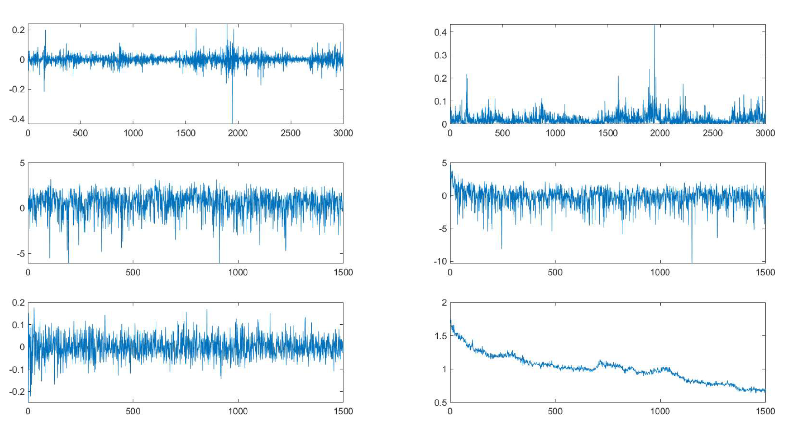
3. Examining the Behaviour of the EUA Carbon Futures Market

The data analysed for the research reported in this paper covers EUA December Futures (Close-of-Day) from early April 2008 until mid-August 2019. Figure 1 outlines the combined data set for EUA Futures price history based upon the Reuters and Quandl Carbon Price Data available at https://www.quandl.com/ (accessed on 28 February). All the analysis prepared has been developed using Microsoft Excel, MATLAB, and the ‘Eureka’ Evolutionary Computing system, as discussed later in the paper.
Figure 2 indicates the frequency histogram of the data with a bin width of €0.50. Based on the statistical characteristics, it does not conform to the traditional bell curve and the data would appear to be non-normal. The standard deviation is 7.07, while the kurtosis is noted to be −0.8779, indicating a fatter distribution than normal with longer tails. Skewness was calculated to be 0.5394, indicating a longer tail to the right.
In this work, we are interested in the normality, or non-normality, of relative variations of price, rather than the value of the price. In this context, Figure 3 shows the frequency histogram of the log of price change.
Figure 4 indicates the real log of price change over the period. Figure 5 is a log plot of randomly generated price data based on an assumption of a normal distribution with identical mean and standard deviation for the real price data. The EMH implies that prices follow a random walk model and that the sum of small independent price movements are taken to have a normal Gaussian Probability Density Function (PDF). Thus, a Gaussian distribution should be expected from the EUA futures signal under the EMH. However, if we compare Figure 4 with Figure 5, we observe that the actual price data does not appear to conform to that of a stationary Gaussian process. Note that the purpose of applying a natural logarithmic transformation is to remove the exponential element of the signal and the purpose of using the forward derivative is to include price changes only.
Figure 6 indicates a Q-Q (Quantile-Quantile) plot of the data. This plots price against probability (vertical and horizontal axis, respectively) and illustrates the expected result under an assumption of normality (green) and actual results based on examination of the historical data (grey). The ‘S’ shape result of the ‘actual’ indicates longer tails than would be considered under an assumption of normality, i.e., a Gaussian distribution.
As auto-correlation reflects the degree of similarity between a time series and its residuals, on the basis of the EMH, one would expect to find no correlation (or memory) across a time series. The Ljung-Box [26] test and Box-Pierce test [27] are both commonly used in ARIMA modelling and are applied to the residuals. Here, the hypothesis being tested is that the residuals of the time series data have no auto-correlation. If significant auto-correlation is not present in the residuals, then the time series is considered to pass the null hypothesis test. For example, the Ljung-Box test can be defined as
Q = N ( N + 2 ) k = 1 L r k 2 ( N k ) ,
where N is the sample size, L represents the number of auto-correlation lags, and r 2 is the squared sample auto-correlation at lag k. The null hypothesis is rejected if
Q > X 1 α , h 2 ,
where inequality (2) represents the chi-square significance level, with α and h being the degrees of freedom.
Results for the 2005–2019 EUA Futures time series compared with randomly generated price data based on an assumption of a normal distribution with identical mean and standard deviation as the real price data, finds that the null hypothesis is rejected for the Ljung-Box test for all residuals examined. The p-value is found to be exceptionally small (<0.05) with very good correlation between the Ljung-Box test and the Box-Pierce [27] test, both returning identical results of 94.51%).
A Wilcoxon Signed-Rank test [28] p-value of 0.97% is obtained for this same data, and the Durbin Watson statistic [29] is 2.002, indicating no correlation in the data. Variance Ratio (VR) testing [30] was also carried out on the time series. A p-value of 1.55% and 1.71% was found based on various day-returns for VR testing. Thus, using such metrics (and others), the null hypothesis can be rejected. This indicate that the price change of the EUA time series between 2005 and 2019 is significantly statistically different to that of a Gaussian distributed time series with identical mean and standard deviation. It may, therefore, be inferred that the EMH is not applicable to the EUA futures market and applying a ‘normality’ assumption does not reflect the actual market characteristics (based on historical market data).
Previously identified limitations in the assumption of a normal distribution have prompted a new range of methods for investigating time series. Among these is the RSRA method [31,32,33], which is based on computing and analysing the Hurst Exponent H. The value of H increases according to a simple power law which provides an underlying connectivity between the Hurst Exponent and fractal geometry in general. Here, H = 0.5 is consistent with an independently distributed system. For 0.5 < H 1 , persistent dynamical behaviour is prevalent and for the range 0 < H 0.5 , anti-persistence behaviour occurs which can be characterised by negative correlations.
Hurst developed this novel way of measuring correlations in data based upon Einstein’s earlier work on Brownian motion. Hurst generalised the Brownian motion equation according to
R n S n = c n H ,
where R n is the range of the first n cumulative deviations from the mean, S n is the series (sum) of the first n standard deviations, n is the number of data points in a time series, and c is a constant. Thus, the relationship between how a random time series scales with respect to time is generalised in Hurst’s equation which documents the scaling relationship between a general process and time by the Hurst exponent H. A logarithmic transformation of Hurst’s equation yields
log R n S n = log ( c ) + H log ( n ) .
Under the assumption that this model is valid for a time series, the graph of log ( R n / S n ) plotted against log ( n ) is characterised by a gradient that is H. In this context, analysis was undertaken on the EUA Futures time series, to determine long-term dependence characteristics. This was achieved by calculating the Hurst Exponent and Fractal Dimension D. Utilising RSRA, the Hurst exponent for the full series is 0.348. This indicates anti-persistence and short-term dependence in the data set. This confirms that the data does not follow a (Brownian) random walk model (i.e., H = 0.5 ). The fractal dimension D was determined to be 1.652.
Figure 7 shows the RSRA plot (green). In all segments of the half and third series, the Hurst Exponent indicates anti-persistence. This compares with a value of H = 0.4859 from research by Feng, Zou, and Wei in 2011 [34], where they found memory effects in the carbon price for the period April 2005 to December 2008. Based upon this research, these characteristics have become more pronounced throughout Phase II and Phase III of the EU ETS, at least for EUA futures.
Prior research by the authors of Reference [35] has demonstrated that the power spectrum of a signal characterises the distribution of the correlation. From this, we can, in turn, estimate long term memory. More power at lower frequencies indicates time correlations over the long term and, therefore, that there is long market memory. If, however, there is more power at the higher frequencies, then we can say that there is evidence of short market memory. A function [35] that characterises the correlations between segments of a time series for a price signal u ( t ) is
u ( t ) u ( t ) U ( ω ) 2 ,
where ⊙ denotes the correlation integral, and ↔ denotes transformation from real space (time t) to Fourier space (temporal frequency ω ). The spectrum U ( ω ) is given by
U ( ω ) = F [ u ( t ) ] = u ( t ) exp ( i ω t ) d t ,
where F denotes the Fourier transform operator. The function U ( ω ) 2 is the power spectrum which characterises the amplitude distribution of the correlation function, from which we can estimate the time span of memory effects. This can also enable us to calculate the auto-correlation function (i.e., the inverse Fourier transform of U ( ω ) 2 ). Thus, if we calculate the Auto-Correlation Function (ACF) of the price increments for carbon price futures, then we can see how much of what happens today is correlated with what happens in the future. Under an assumption of the EMH, there should be no memory and, therefore, no correlation. Thus, we could expect the power spectrum to be a constant and the ACF a delta function. In this context, the ACF for price changes of EUA futures (2005 to 2019) was calculated and is shown in Figure 8.
From Figure 8, the ACF of the log price changes (i.e., the lower-left plot) is quite indistinct, indicating that the low frequencies within the price signal has little effect on the correlation. The power spectra of the data (i.e., centre-left and -right plots) are not constant and have distinct peaks at the medium and higher frequencies. However, the absolute log plot (top-right) shows a power law at the low frequency end of the spectrum. This indicates that there are correlations within the data and memory effects at play. The ACF of the absolute log price changes (i.e., lower-right plot) illustrates that there are correlations at around 750 and 1000 days, with an irregular decline up to 1500 days.
Comparing Figure 8 against what should be expected under the EMH (i.e., a constant power spectrum and an ACF that is a delta-type function), we see that the log price movements has a better long-term memory than one would expect under the EMH. Indeed, correlations of any type, whatever the time scale, invalidates the independence assumption of the EMH. Figure 8 is, therefore, an example that indicates a very different behaviour of the EUA futures time series to that of an EMH model.
The Ljung-Box and Box-Pierce Q-tests for Auto-Regressive Conditional Heteroskedasticity (ARCH) on the EUA Futures time series alone, shows Q-Stat results of 98.2% and 98.1%, respectively, with exceptionally small p-value’s, indicating that volatility in financial markets is non-constant, that the returns are Heteroskedastic and behave according to ARCH. Applying lags of 750 and 1000 days corresponds to the results shown in Figure 8. Thus, in analysing carbon futures data across a variety of approaches, it is demonstrated that the EUA Futures time series is non-Gaussian, the PDF of log price changes is not Gaussian and price changes are not fully independent. Secondly, it is shown that the price signal is non-stationary. Thus, the time series data is argued to be rendered incompatible with the random walk approach and the EMH. An FMH approach is, therefore, proposed, and we consider the carbon price change field to be highly non-linear, subject to Lévy flights, sensitive to exogenous shocks and that these shocks may have long-term effects. Memory was tested by observing correlations in the data, and this demonstrates long-term market memory at play.

4. Stochastic Field Theory and the Determination of an Investment Index

In this section, we discuss the background to Einstein’s Evolution Equation, the Random, Efficient, and Fractal Market Hypotheses and the approach to the development of a carbon market future trend indicator. This is a summary only, as this work is detailed more fully in an associated publication by the authors of Reference [36]. Interested readers should refer to this paper for a fuller derivation of the underlying hypothesis and its application to financial markets in general. The findings from the application of this approach to EU ETS EUA carbon futures trading is the focus of this particular paper.

4.1. Einstein’s Evolution Equation

Let p ( r ) denote a PDF, where
p ( r ) d n r = 1 .
The PDF characterises the position of particles in a n-dimensional space r R n . At any instant in time t, the particles are taken to have behaved according to some ‘random walk’ resulting from ‘elastic scattering’ processes over a period of time < t . Let u ( r , t ) describe the density function (the number of particles per unit space of dimension n) associated with a (canonical) ensemble of particles generated by the random walk process. For initial condition t = 0 , suppose we have then have an infinitely small concentration of particles located at origin r = 0 , say. We can then consider the density function at t = 0 to be given by u ( r , 0 ) = δ n ( r ) , where δ n ( r ) is the n-dimensional Dirac delta function.
At some short time later t = τ < < 1 , the density function will be determined by the PDF governing the distribution of particles after a (short term) random walk and the particles will be distributed in space according to the PDF p ( r ) , i.e., u ( r , τ ) = p ( r ) . However, this results can be expressed as
u ( r , τ ) = p ( r ) u ( r , 0 ) = p ( r ) δ n ( r ) = p ( r ) ,
where ⊗ denotes the convolution integral over all r . In this context, the PDF p ( r ) , therefore, represents the response associated with a random walk process and can be considered to be the statistical equivalent of an Impulse Response Function (IRF). Thus, at some later time t + τ , the density field will be given by
u ( r , t + τ ) = p ( r ) u ( r , t ) ,
which is Einstein’s Evolution Equation (EEE) [37] and is an example of a continuous time random walk model.
From Equation (9) and for a source function s ( r , t ) , EEE can be written as
u ( r , t + τ ) = p ( r ) u ( r , t ) + s ( r , t ) .
The financial time series models applied to carbon trading, as presented in this paper, are ultimate, all derived from Equation (10). Thus, Equation (10) is the basic stochastic field equation for the stochastic field u ( r , t ) which unpins all of the models developed. A financial time series is taken to be a time signature associated with the field u ( r , t ) .

4.2. The Approach to Predicting Market Trends

Deterministic models can be of value in the understanding of some micro-economic systems; however, in ‘large markets’, where they are subject to external and unquantifiable influences, we are required to describe behaviour in terms of functions of random variables. These systems are generally complex because the market responds to itself and has non-linear behaviour in the sense that the system includes a feed-back. Thus, we consider price change to be highly non-linear, sensitive to exogenous shocks and where market ‘memory’ exists. This approach represents a methodology in which principal aim is to aid in the prediction of future price behaviour, i.e., bull or bear trends.
The time dependence of a density field is described by an n-dimensional version of EEE, which is taken to be a model for carbon futures price behaviour. The Generalised Kolmogorov-Feller Equation (GKFE) is taken to be a representation of EEE for a memory function m ( t ) and and is known that memory functions can be used to study the fractionalisation of general kinetic equations, such as random walks and Lévy flights. EEE in its fractional form is considered to be a result of introducing non-Gaussian distributions as ‘governors’, subject to the assumption that all of these involve independent and elastic interactions. A self-affine model can be considered, as this is equivalent to a Lévy distribution type system with a δ ( t ) memory function. Consideration of the Random Walk Hypothesis (RWH), the EMH and FMH, each being taken in the context of EEE, show that [36]:
  • The RWH is compounded in the case when p ( r ) = δ n ( r ) ; therefore, EEE is reduced to the simple form
    u ( r , t + τ ) = u ( r , t ) + s ( r , t ) .
  • The EMH is compounded in the case when p ( r ) P ( k ) = exp ( c k 2 ) for a real constant c, i.e., when the PDF is a Gaussian function. In Fourier space, we can write EEE as
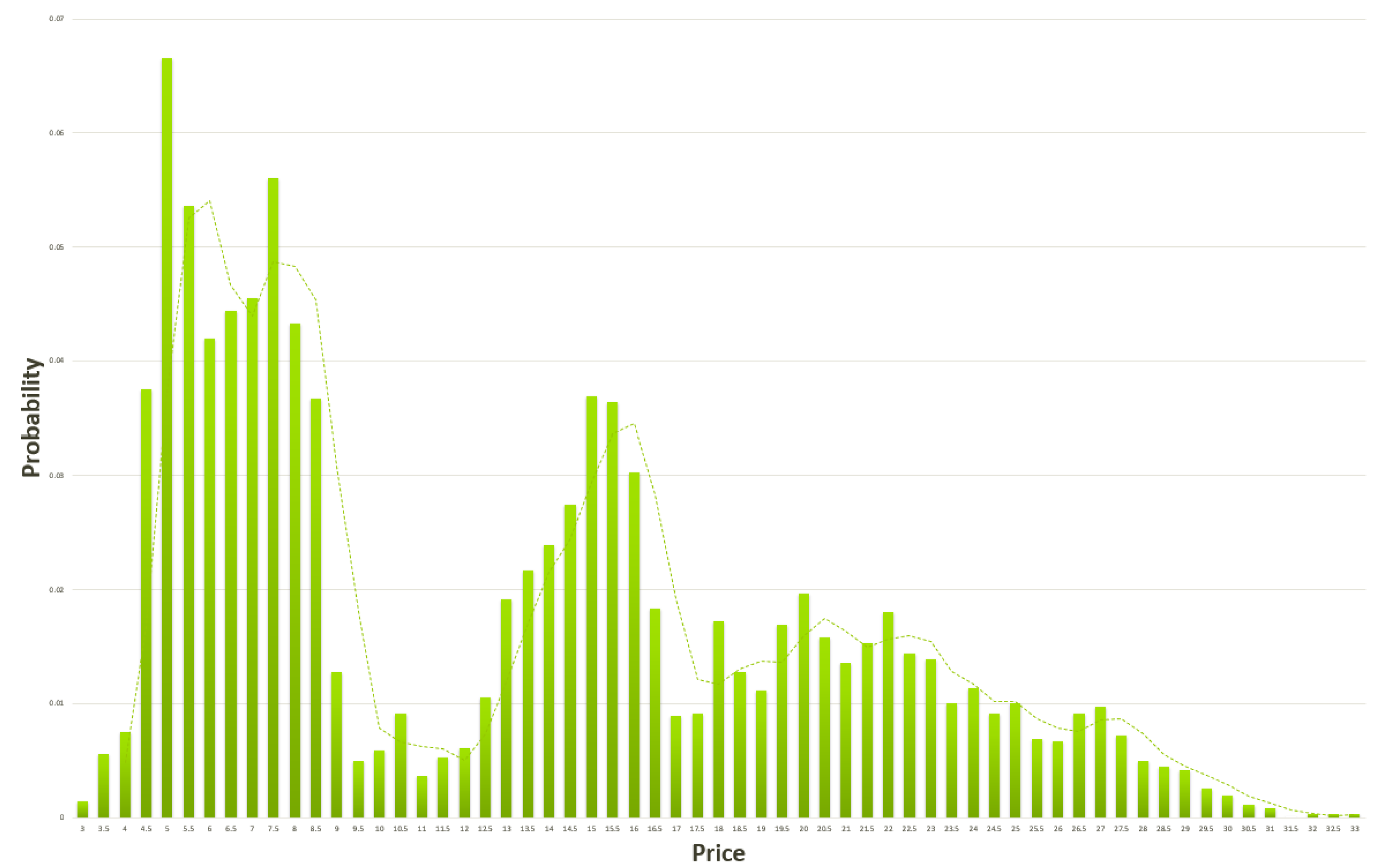
    U ( k , t + τ ) = exp ( c k 2 ) U ( k , t ) + S ( k , t ) .
  • The FMH is compounded in the case when p ( r ) P ( k ) = exp ( c k γ ) , 0 < γ < 2 where γ is the Lévy Index for a real constant c, i.e., when the PDF is Lévy distributed. In Fourier space, the evolution equation is then given by
    U ( k , t + τ ) = exp ( c k γ ) U ( k , t ) + S ( k , t ) .
    The Lévy distribution has a Characteristic Function (CF) which is a generalisation to the form
    P ( k ) = exp ( c k γ ) , γ ( 0 , 2 ) .
    For γ = 2 , a Gaussian PDF is obtained; for γ = 1 , the PDF is a Cauchy distribution, and, with γ = 0 , the PDF is a delta function. Specifically, for r R 1 , it can be shown that, for γ = 1 [36],
    exp ( c k ) 1 π c c 2 c 2 + x 2 1 x 2 , x ,
    and, for γ ( 0 , 2 ) [36],
    exp ( c k γ ) 1 x 1 + γ , x .

4.3. The Lyapunov Exponent, Volatility, and the Lyapunov-to-Volatility Ratio (LVR)

The Lyapunov exponent can be derived from EEE [36], and, for a continuous time series x ( t ) with an initial value x 0 , the (leading) Lyapunov Exponent λ can be shown to be given by
λ 1 t ln δ x ( t ) p δ x 0 p ,
where p denotes the p-norm. In the context of EEE, the Lyapunov Exponent can, therefore, be considered to be an intrinsic metric that plays a similar role and yields a complementary measure to the Hurst Exponent and the Lévy Index, for example. However, the Lyapunov Exponent can be computed more effectively because it does not require the application of a regression algorithm. For this reason, the approach considered in this work focuses exclusively on the application of the Lyapunov Exponent.
For a discrete time series which is based on some iterative process in which an error occurs denoted by ϵ ( t n ) , n = 1 , 2 , , N and is characterised by exponential growth exp ( λ τ ) where τ is the sampling rate, the Lyapunov Exponent can be written in the form [36]
λ = lim N 1 N τ n = 1 N ln ϵ ( t n + 1 ) ϵ ( t n ) .
It is then apparent that, if λ is negative, then we can state that the iterative process is stable since, for n > > 1 , ϵ ( t n + 1 ) / ϵ ( t n ) < 1 , and, thus, ln [ ϵ ( t n + 1 ) / ϵ ( t n ) ] < 0 . If λ is instead positive, then we can say the iterative process is divergent. In this context, for a discrete time series u n > 0 n with a finite number of samples N, we can compute the Lyapunov exponent using
λ = 1 N τ n = 1 N ln u n + 1 u n .
If a financial time series is predicated on Equation (10), then we can determine the Lyapunov exponent using Equation (19), where ϵ ( t ) is taken to be an integral over all space [36]. This includes EUA futures data when λ can be calculated on the basis of a look-back window in order to generate a sequence of the Lyapunov Exponents for an array of size of N. The product N τ scales the calculated values of the Lyapunov exponent. If u n + 1 > u n , n > > 1 , then λ > 0 , and, if u n + 1 < u n , n > > 1 , then λ < 0 . Therefore, we can say that, regardless of scale, the zero crossings associated with changes in the value of λ is an indicator of a change in the trend of EUA futures. This is the underlying basis for the approach considered in this work.
We note that, since we can write Equation (19) in the form
λ = 1 N τ n = 0 N ln u n + 1 ln u n ,
and that
ln u n + 1 ln u n τ d d t ln u ( t ) ,
then, for the continuous time series function u ( t ) , t [ 0 , T ] ,
λ 1 T 0 T d d t ln u ( t ) d t = 1 T ln u ( T ) u ( 0 ) .
The computation of the Lyapunov exponent through application of Equation (19) relies on the size of the moving window that is used. The trading delay, which is proportional to this size of the look-back window used, can be determined as required depending on the duration and nature of the time series being examined. The zero-crossings of the signal can then potentially be used to estimate changes in the trends in the EUA futures time series. This is because the ‘zero-crossings’ associated with the Lyapunov exponent provides the positions where there is a transition in the nature of the price trend. Further, given that the Volatility of a time series describes its ‘stability’, this suggests that we scale the Lyapunov exponent with the volatility σ to produce a LVR indicator
λ σ = λ σ ,
where σ is defined by
σ = ln u n + 1 u n 2 ,
and τ = 1 / N , making λ σ scale independent. In this case, the value of λ σ indicates not only changes in the direction of a trend but also the stability of the trend. The MATLAB functions for computing the Lyapunov Exponent and the Volatility are provided in Appendix A.1 and Appendix A.2, respectively.
The positions in time at which the zero crossings are evaluated depend on the accuracy of the algorithm used to compute λ σ , i.e., in Equation (23). This itself depends on the inherent noise within the EUA futures data. As a result, this can yield errors relating to the exact positions where the zero-crossing occur, especially those related to changes associated with short time ‘micro-trends’; albeit that the term ‘noise’ must be understood to include legitimate price values. In order to overcome this, an approach is taken which is based on filtering u n using a moving average filter which can be written in the form (using a continuous time representation of the functions)
u ( t ) : = w ( t ) u ( t ) ,
where
w ( t ) = 1 / W , t W 0 , t > W ,
and W is the given length of the moving window which computes the mean of the windowed data. The moving average filter (which is given in Appendix A.3) pre-filters the data u n with a selected window of size W. It is also worth noting that an option for post-filtering λ σ ( t ) is also required to control the dynamic behaviour. We, therefore, take a similar approach for post-filtering, where we consider the output
λ σ ( t ) : = w ( t ) λ σ ( t ) ,
where
w ( t ) = 1 / T , t T 0 , t > T ,
and T defines the length of the post filtering moving window, T W . In other words, we again apply the same approach to filtering the data, but, this time, we filter the LVR signal, whereas the pre-filtering signal filters the price signal. The MATLAB function for computing this filter is provided in Appendix A.3.
By computing λ σ ( t ) , with t being the position of the window under consideration, zero crossings are given by the function
z c ( t ) = + 1 , λ σ ( t ) < 0 & λ σ ( t + ε ) 0 ; 1 , λ σ ( t ) > 0 & λ σ ( t + ε ) 0 ; 0 , otherwise . ,
where ε is a small variation in time.
The function z c ( t ) generates a sequence of Kronecker delta functions in which polarity indicates a point (in time) where a price signal can be expected to be positive or negative, i.e., the price is expected to go up or down. The function identifies the zero-crossings associated with the end of an upward trend and the start of a downward trend as is the case when z c ( t ) = 1 and the end of downward trend and the start of an upward trend as the case z c ( t ) = + 1 . This provides an approach to forecasting the trending behaviour of the EUA futures time series in which exploration is presented in the following section.

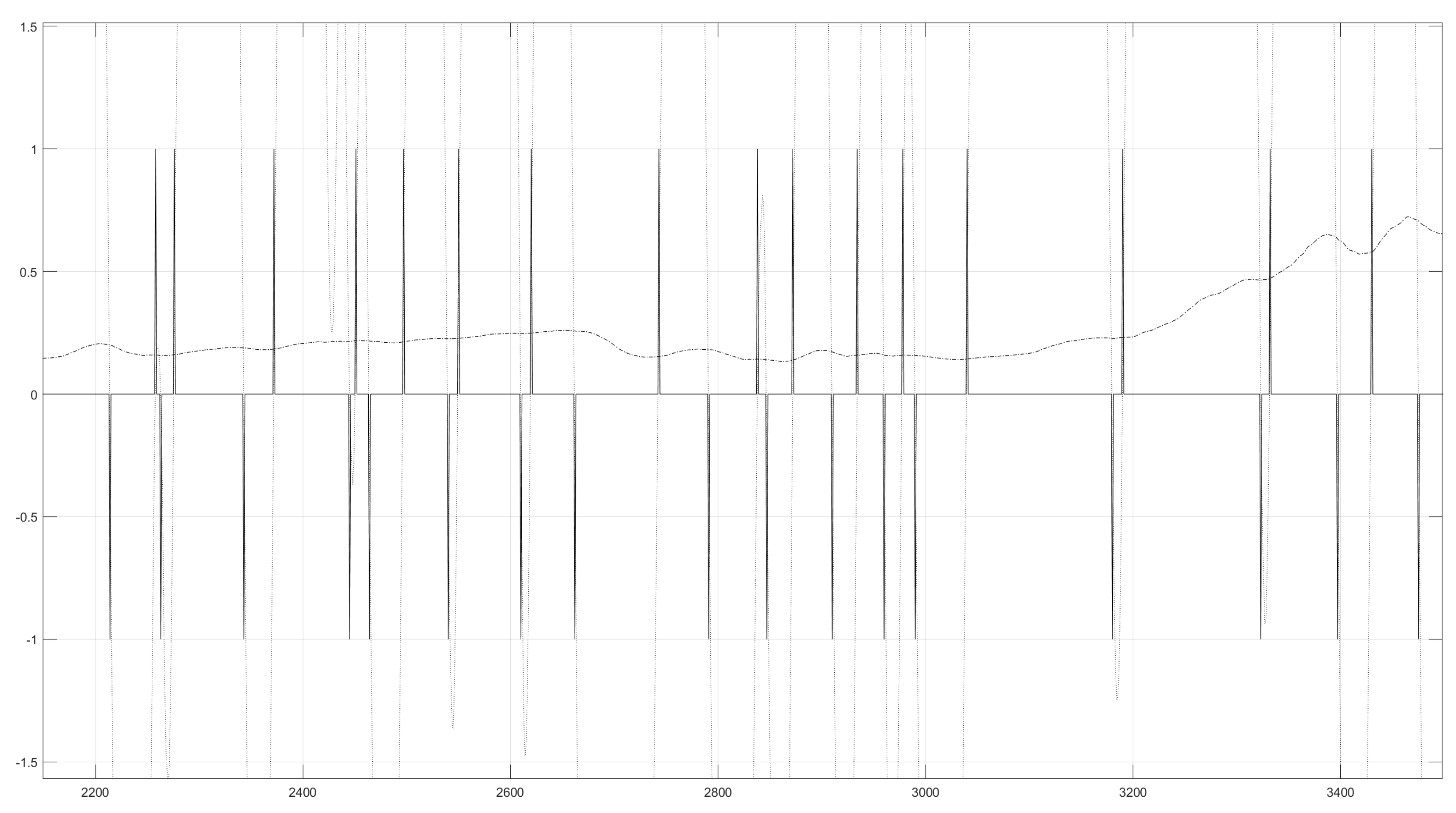
5. Carbon Futures Trading

In market trading, backtesting allows us to determine how well a trading strategy would have done after the event. It allows us to understand the benefit (or otherwise) of some trading strategy by assessing how it performed using historical price information. In examining carbon futures trading over the period as shown in Figure 1, an evaluator function was utilised to evaluate the indicator performance associated with the zero-crossings signature of the LVR. This operates on the premise that the price change is reflected by the difference between the first and last points in a predicted trend, if the prediction is accurate. Thus, we argue that, when z c ( t ) > 0 , and the trend is upwards, the price change between one point in time and the next point should be generally positive, thereby representing a price increase. Similarly, when z c ( t ) < 0 , and the trend is negative, the price difference between a point in time and the next should be negative (in general), thereby representing a price reduction. For the positions in time where this occurs (for any length in the time series L examined), the entry and exits points are taken to be correct, or else, they are taken to be incorrect.
The accuracy based on this backtesting approach is calculated as a percentage in terms of the correct prediction of entries and exits. This indicator is based on an LVR algorithm compounded Equation (23) and scripted for use in MATLAB on a moving window basis as given in function ‘Backtester’ provided in Appendix A.5 which uses the function ‘Evaluator’ given in Appendix A.4 to evaluate the accuracy of the strategy. The backtesting function provides optionality on the sizes of the filtering windows W, T, and L for any time series. The function also normalises the data so that it can be presented on a scale equivalent to λ σ [ n ] . The function then provides a graphic of u n , λ σ [ n ] and z c [ n ] and collates the trend predictions in terms of trend identification accuracy.
Figure 9, Figure 10 and Figure 11 present sample results from the evaluation of the first 3500 elements of the EUA (Close-of-Day) futures. The three examples given are for different values of the variables W, T and L using function ‘Backtester’ as follows: Backtest No. 1 - Backtester(10, 10, 3500), Backtest No. 2 - Backtester(20, 10, 3500) and Backtest No. 3 - Backtester(30, 10, 3500). The combined predictive long/short accuracy is 47.05%, 61.11%, and 75.64%, respectively. Figure 9, Figure 10 and Figure 11 shows λ σ [ n ] (dotted line), the pre-filtered time series u n (dot-dashed line), and z c [ n ] (solid line) which identifies the zero-crossings of λ σ [ n ] .
Based on Figure 9, Figure 10 and Figure 11, it is demonstrated how trend prediction accuracy improves by increasing the pre-filtering window applied, i.e., prior to computation of the LVR. This can be explained by the fact that the pre-filtering reduces the ‘noise’ associated with the time series; therefore, ‘smooths’ the price signal. All other considerations aside, therefore, we can say that this approach provides a clearer trend indicator, with more accurate results which is observed in the variance between Figure 9, Figure 10 and Figure 11.
In the figures shown, the solid line (i.e., dark vertical ‘impulses’) represents z c [ n ] , i.e., polarity changes associated with λ σ [ n ] . Here, a positive ‘spike’ indicates a long market view, with a negative ‘spike’ representing a short market position. The dash-dot line (i.e., the line between 0–1 on the y-axis) represents u n , which is the filtered time series data. This is a filtered version of the raw price information from the original time series but smoothed to reduce the signal ‘noise’ (albeit in this context, the term ‘noise’ used here is actually a legitimate market price values). The u n signal can be used visually to interpret the suggested investment entry and exit points (i.e., λ σ [ n ] ) relative to future price movements, with an upward trend being a market price increase and a downward trend being market price decrease. The dotted line shows the LVR λ σ [ n ] after being rescaled. The strength and stability of this LVR is used to inform the ‘confidence’ of any trend prediction, or related investment position, given that this metric is based on the Volatility and the Lyapunov Exponent, both of which can be used to characterise the stability of a signal with respect to its future behaviour.
To optimise pre-filtering and post-filtering selection for the carbon futures time series, an approach was taken to utilise a surface mesh plot (hereinafter referred to as a ‘WT-map’). This is an output plot which shows the accuracy of a backtest, for different values of W and T. From a WT-map, it is possible to determine optimal parameters for W and T in terms of the predictive accuracy for the backtest. Figure 12, Figure 13 and Figure 14 show WT-maps of the combined accuracy as a function of the pre- and post-filtering look-back window sizes W and T, respectively, each for a variations of length L for 1000, 2000, and 3572 (i.e., this being the full time series). MATLAB scripting for the analysis used in this paper is located in Appendix A.
The W T -maps of the type given in Figure 12, Figure 13 and Figure 14 enable optimal values of the pre- and post-filtering windows to be established. This is achieved by attempting to find the lowest value of W and T (i.e., the least noise filtering and trading lag, respectively) which maintain a combined accuracy (entry and exit accuracy) compatible with an expected, or acceptable, confidence (over a given time scale). From Figure 12, the variables W and T are optimised for W [ 46 , 49 ] and T [ 10 , 13 ] where the highest plateau of the W T -map occurs, the height being reflective of the percentage accuracy for the backtest. This result is obtained for L = 1000 for the Close-of-Day EUA futures market price.
Figure 13 and Figure 14 have also been included to visually represent the impact of increasing L from 1000 to 2000 and, finally, to 3572. Accuracy values associated with the W T -maps with respect to a value of L given by 1000, 2000, and 3572, are 100%, 84%, and 82%, respectively. From these results, we clearly observe a drop in the accuracy with increasing window size L. This can be said to be somewhat intuitive, given that with longer durations, we are effectively crossing EU ETS ‘phases’, each having different rulesets and characteristics. Interestingly, however, despite reduction in the predictive accuracy for increasing values of L, optimal values of W and T (at least for entry/exit and exit/entry) remains in the broad range similar to that as outlined above for Figure 11 (i.e., W [ 46 , 49 ] and T [ 10 , 13 ] ). Thus, the approach taken (through the computation of W T -maps) determines the optimal range values of W and T (for increasing values of L) in respect of trend prediction accuracy.
To consider the predictive capability for specific EUA futures products (rather than using a merged data set), additional analysis was undertaken on the individual time series’ which is outlined below in Table 1. The purpose is this is primarily to consider the optimal values of W, T and L on product specific data sets and to examine comparative returns on a product-by-product basis. Table 2 indicates the predictive performance results derived from the backtest evaluator (as described earlier), based on W = 48 and T = 11 , with L equal to the length of the respective product time series being examined.
In assessing performance results, the application of the dynamic filtering operation has considerable impact on the predictive capacity of the approach presented. Without application of this filtering, the accuracy for determining the correct trends for going long or short remains relatively poor. To output the levels of predictive accuracy required for commercially viable rates of return, the filters must be applied within a certain window length. For the data considered here, it was demonstrated that the pre-filter needed to be a minimum of ∼30 to maintain accuracy and was optimised at or around ∼48. Without filtering, backtesting shows that the entry/exit accuracy was ∼50%. However, with suitable filtering, a predictive accuracy in the order of ∼85% is achieved. This is based on 35 years of combined EUA price information and analysis of a variety of futures products.
To carry out an initial assessment for out-of-sample backtesting, Figure 15 shows the trading signals from the first 1000 ticks (i.e., from the 1 December 2004 to the 16 February 2011) for the EUA spot market. EUA spot market data over this range was available through the Point Carbon data set. However, this was not previously considered as part of the development and performance analysis of the model as the focus was exclusively on the futures market. While further research is recommended to fully evaluate out-of-sample backtesting, the results derived from Figure 15 indicate a combined predictive accuracy of 85.71%. This result is consistent with the average results from the in-sample tests, and, as a preliminary result at least, would suggest equivalent in-sample and out-of-sample results should be expected.

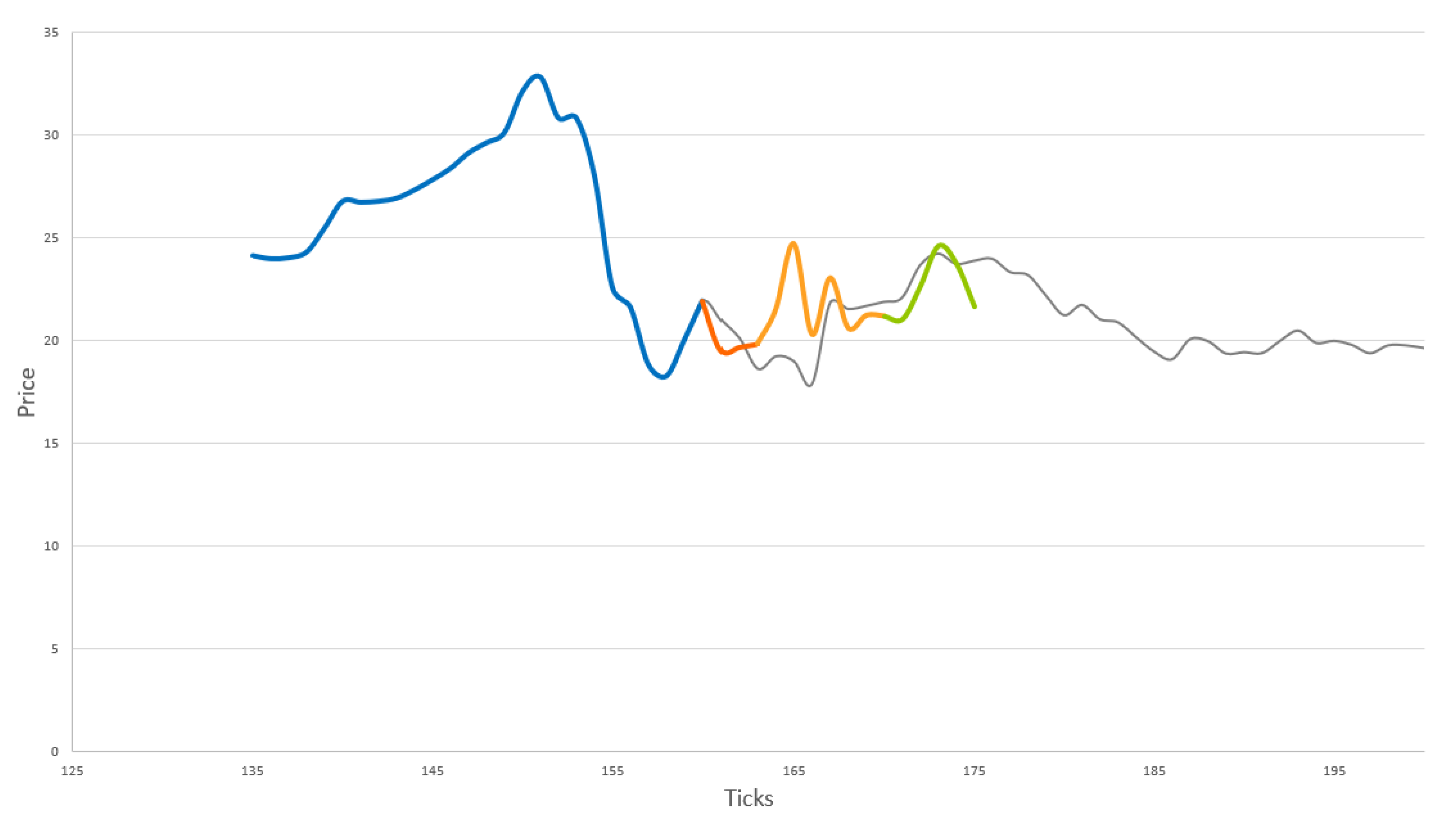
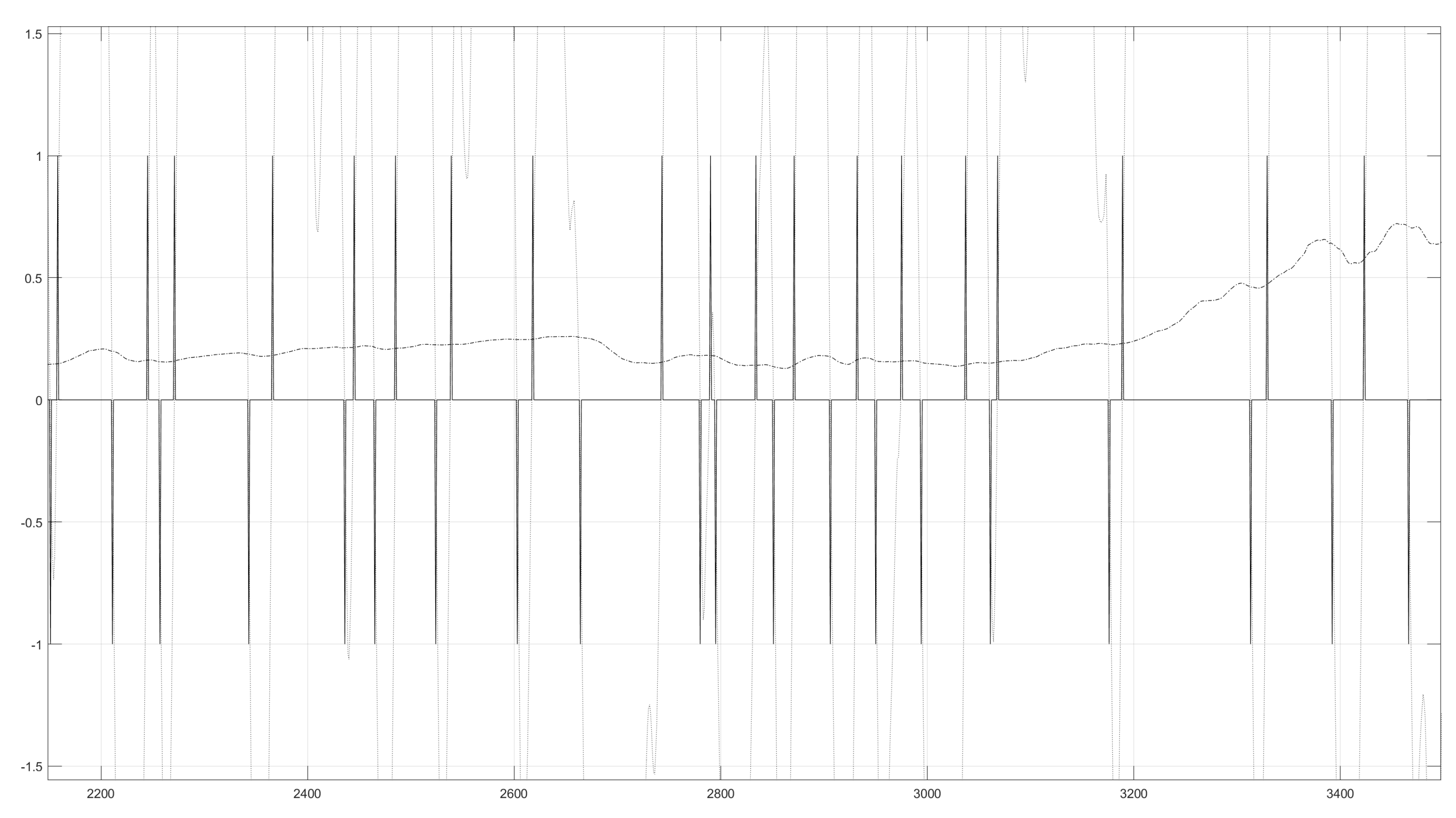
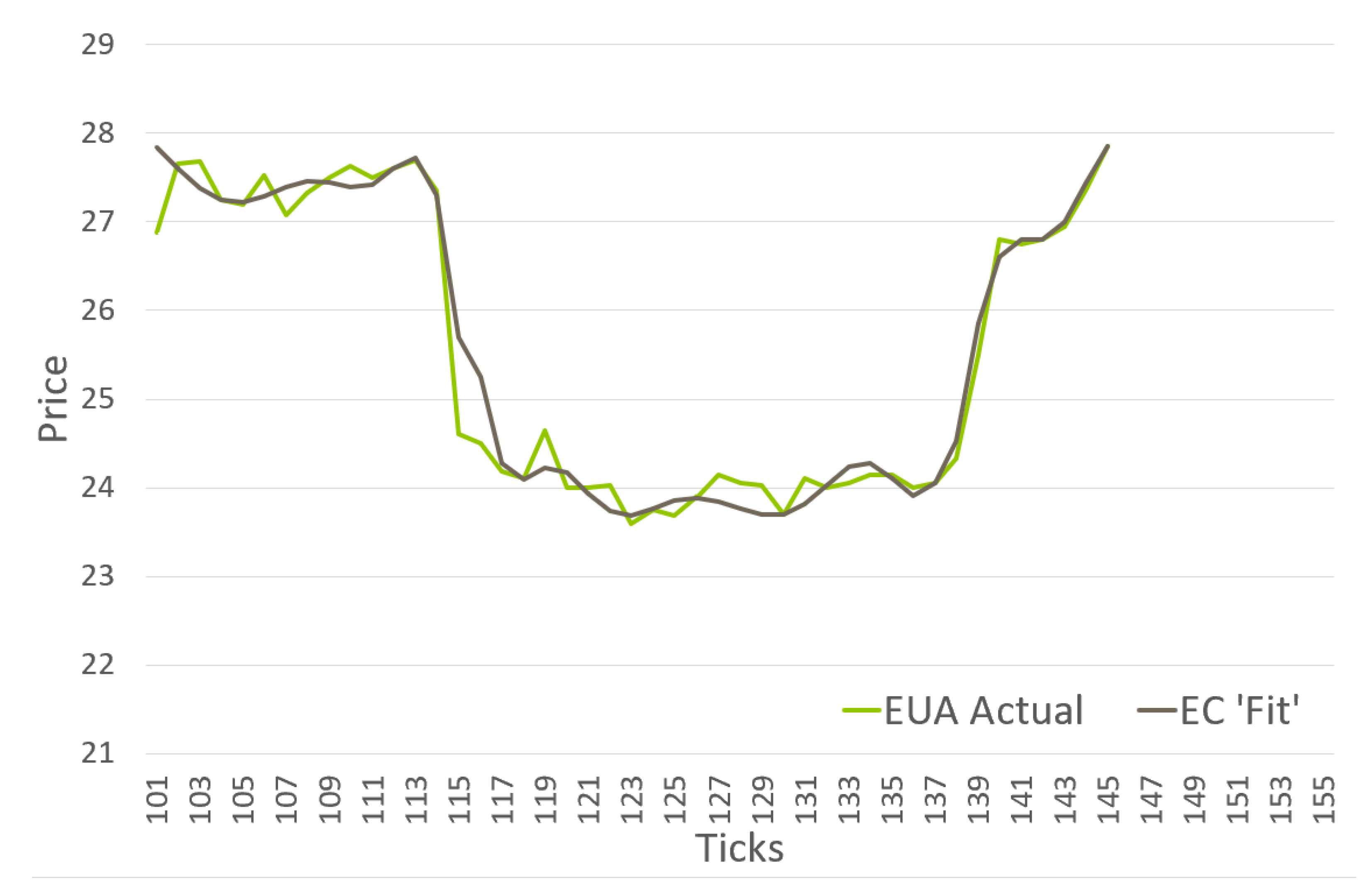
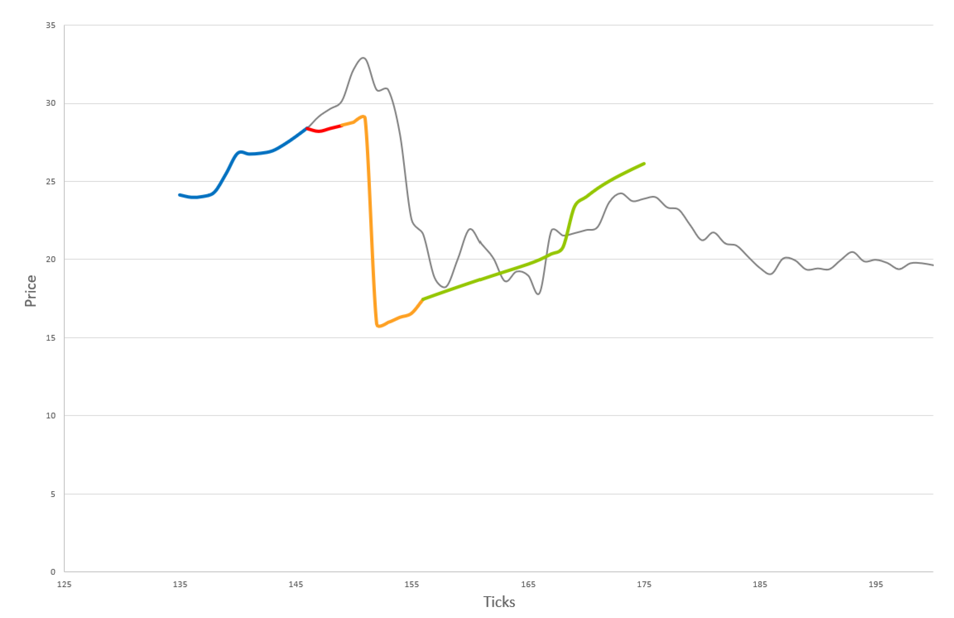
6. Future Price Prediction

The analysis presented so far makes a prediction on the future movement of the time series, this being up or down to indicate a long or short position, respectively. It does not indicate the scale of any future price movement, which would also be a useful aid for any market participant. In theory, this could have a range of market applications, including options pricing, for example. However, within this scope, we consider it of potential use in informing when, specifically, to execute a buy/sell trade within a flagged trend (i.e., when the intention is to take a new long or short market position), using the zero-crossings. The underlying hypothesis to this approach is that a steady LVR amplitude may reflect intervals of stability in the dynamic behaviour of the carbon futures signal; therefore, some method may be able to exploit this (temporary) condition to provide short-term predictions on future pricing. This could then be used to guide specific trade execution points over some short-term future time horizon. By default, only an estimate of any future price movement is ever possible. However, the lower the Volatility of the carbon data, at a particular point in time, the less likely it is to exhibit large random variations (i.e., a Lévy flight), at some (short) distance in the future. In this context, we can hypothesise that the greater the value of the LVR, the more chance there is that a future price prediction will have some degree of confidence associated with it. This may then help to inform a trading approach within a trend based on an expectation of the short-term price movement.
In this section, we consider the hypothesis that Evolutionary Computing (EC) can be used as a price predictor, provided certain ‘stable’ market conditions prevail, as indicated by the LVR when it is broadly constant and with a ‘strong’ amplitude. The rationale for this is that, by taking EEE in the form given in Equation (10) and integrating over r , then, for p ( r ) = δ n ( r ) , we obtain
u ( t + τ ) = u ( t ) + s ( t ) ,
which is a continuous time model for the RMH. This model states that the price tomorrow is likely to be close to today’s price which is identified by large amplitude for the LVR when economic conditions are most likely to prevail and, thereby, provides the possibility to use an EC to estimate future (short-term) price values. The trading strategy is, therefore, to generate representative equations for historical price movements over a period of relative LVR stability using EC. When these enabling conditions exist, it is hereinafter referred to as a ‘LVR EC Period’.
For each additional tick, an evolutionary computed equation can be used to account for actual price data which in turn, provides an updated solution for the short-term price horizon. In effect, this uses a similar moving window process with options to utilise the window for some moving fixed (short) length or to expand the window as new information is received, so as to avail the full length of the LVR EC Period. Under this approach, we consider that the LVR can be used not only to enable an approach to estimating future trends but also to signal when EC may be applied successfully in order to generate some estimate of a future (short-term) price(s).
Within the field of EC itself, ‘Eureqa’ is a software platform first developed by Cornell University [38]. The basis of the approach is to generate increasingly better best fit functions to replicate some dataset [39]. It is, therefore, an AI-based engine which uses evolutionary computing [40]. It randomly creates equations via sequences of mathematical building blocks based on a combination of common functions. Inputting historical price data for LVR EC Periods, we can, therefore, generate a ‘formula’ using Eureqa which simulates the (segmented) time series data. By way of a case study, a solution was obtained after 193,949 iterative generations, which gave a correlation coefficient of 0.99199302, an R 2 of 0.98253994, a mean absolute error of 0.14053763 with complexity of 83. The ‘fit’ of this solution (grey), versus the actual price (green), is illustrated in Figure 16.
The formula generated by Eureqa in this example to ‘fit’ the actual price data shown in Figure 16 is
f ( t ) = 174 + 0.00938 t ¯ ( t , 8 ) + 3.83 mod ( t , 1 ) , 0.33 ) + 0.000224 t ¯ ( t , 8 ) 2 mod ( delay ( t , 4 ) , 0.33 ) erf ( tan ( 0.215 t ) ) 2.36 delay ( t , 1 ) 0.185 mod ( delay ( t , 4 ) , 0.33 ) tan ( 0.215 t ) ,
where t ¯ denotes the moving median function, and mod, delay, and erf denote the modulus, delay function, and the error function, respectively.
In this example, there is no indication of future pricing; we have simply produced a formula to replicate the price signal from the data provided. However, we can now consider future price prediction by utilising the discretised version of the Eureqa solution given by Equation (31). In this manner, we can generate predicted prices at some future (short-term) time step in the future for t N + 1 , t N + 2 , t N + 3 , , where N is the length of times series used to generate the Eureqa output. Taking, for this example, N = 44 (i.e., the duration of the LVR EC Period up to that point in time), we can, therefore, generate price expectations for the days that follow. From Figure 16 and Tick 146, let us say that a trader looks to utilise EC to predict the price movement for the following day(s). The purpose here is to identify some imminent price fall, in order to sell for the maximum possible gain. Therefore, if the future price indicates a rise (i.e., within the ‘noise’), the trader would wait until the future (short-term) price is predicted to trend downwards, thereby selling at a price ‘peak’. Figure 17 indicates the price prediction results at Tick 146, using a look back window of 45 (i.e., after the commencement of the LVR EC Period).
The use of EC, as given in this example, indicates the trader should consider exiting their position in the proceeding days, ideally at Tick 151, where the associated price is predicted to be €29.03 (using EC), before the expected sharp drop. While the actual price turns out to be €32.85, the interesting observation is that this price prediction correctly estimates the price peak (albeit not the exact value) and the future order of magnitude of the price fall. As shown in Figure 18, at Tick 160, EC indicates a stable but noisy short-term future price. At Tick 161, the LVR drops below + 3 and this LVR EC Period comes to an end. Thus, we can consider the conditions enabling this approach to have ceased and the trader would hold their exited position and await the next (bear) market signal (via a zero-crossing).
Due to the manual nature of running Eureqa for each time step (i.e., sequential Ticks) and within every LVR EC Period, not all individual time series’ were analysed on a per-product basis. However, to evaluate the benefit (or otherwise) of an EC approach, analysis was carried out to compare the returns using EC, against those achieved without. This was carried out using the 2005–2019 time series. The main point of note, is in regard to the relative performance of each result to the other and not necessarily the absolute return. Analysis found that there was a 13% comparative improvement in returns when trading using with the LVR and EC to those trading with the LVR alone.

7. Summary of Results and Comparison with Other Approaches

Table 3 below summarises the trend prediction accuracy based on the backtest evaluator, for the EUA futures 2005–2019 time series and the individual data sets based on specific EUA futures products (all with a December expiry).
Based on the results from Table 3 and across all time series’ data sets evaluated, the average long, short, and combined trend prediction accuracy was 86.66%, 87.41%, and 87.03%, respectively. Table 4 illustrates the Return on Investment (ROI) utilising the model (without EC) against a buy and hold strategy over the corresponding period for each futures product.
As a result of the mandatory participation in the EU ETS market and a lack of external investor activity over the period to which these products relate (due to commodity price collapse arising from over allocation), a baseline ‘market’ performance for ROI expectation was not able to be established for the period. As a benchmark index, over the last 10 years, the average annualised return of the S & P Goldman Sachs Commodity Index (GSCI) was 8.8%, while, between 2005 and 2019, the benchmark annualised return of the S & P 500 was 10.48%. This clearly indicates that, based on historical data, carbon trading would be limited to mandatory participants only, as it was.
Table 4 indicates that, based on historical market performance, the approach presented here outperforms ‘buy and hold’ strategies but does not compare favourably (other than for EUA 2009) to wider S & P 500 benchmark returns. However, analysis of the overall time series and per product data (without EC), indicates that the use of the model for mandatory participants provides a substantive reduction in losses relative to a basic buy and hold strategy (in a bear market), and/or provides greater returns than a buy and hold strategy in a bull market. For non-mandatory speculators, with EUA carbon pricing expected to increase ten fold between 2010 and 2030 and twenty fold to 2050 to support the de-carbonisation of economies [41], the future opportunity becomes more pronounced than looking at simple historical performance.
In 2019, one fund launched an environmental investment fund focusing specifically on investing in global liquid and regulated carbon markets, with the EU ETS being one. They cite a 9% annualised return over the period 2012 to 2018 based on their trading strategy [42]. This equates to a 173% return on the original investment after the 6-year period. Applying a backtest as presented here, over the same time period, returns of 279% were generated, while a simple buy and hold strategy alone indicated a return of 219%. A Sharpe Ratio of 1.25 was noted, relative to 0.72 and 0.87 for global equities and bonds over the period [42].
EC may support increased correlation between trend prediction and net profitability. However, the example figures provided here do not include its use for improving performance in respect of returns on investment. Thus, the key conclusions to be drawn from these results are that:
(i)
an EC (or other) solution to trade execution timing is required (at least for commercially viable levels of return);
(ii)
reductions in the value of W (along with the LVR amplitude to support trading decisions) supports a more profitable return (in most cases) than a value of W optimised for trend prediction alone (without EC). To evaluate the benefit (or otherwise) of EC, analysis was carried out to compare the returns using EC against those achieved from the various approaches outlined previously. This was carried out using the 2005–2019 time series and Table 5 presents the comparative returns.
The principal point of note in regard to these results, is the relative performance of each result to the other, not necessarily the absolute return. While further research is required to evaluate EC performance improvements on a per-product basis and per-trading strategy basis, preliminary results suggests that:
(i)
there is validity in using EC in the LVR EC Periods;
(ii)
trading using this approach improves returns by overcoming the issue of lag and noise around the trade execution points within a trend;
(iii)
this approach may provide ROI expectations well above that otherwise expected in the market and/or comparable with wider benchmarks, even while overall market performance was substantially lower.

8. Discussion

Analysis of the EUA Futures time series data from 2005 to 2019 indicates clearly that the data is non-normal. This is consistent with prior work by Feng, Zou, and Wei [23] in 2015 and other prior research on EU ETS Phase I spot price behaviour [6,7,8]. Further analysis was undertaken on the data set to determine long-term dependence characteristics. The Hurst exponent was found to be 0.348, which indicates anti-persistence and short-term dependence. This compares with that of 0.4859 from previous research [34], indicating that these characteristics have become more pronounced.
From all available research, it is noted to be particularly hard to predict the price futures of carbon due to the non-linearity, underlying fundamentals and the complexity of the time series in general. Whereas quasi-deterministic models may be an aid in the modelling of small scale market systems, in larger-scale markets, such as the EU ETS, especially those subject to external and often imperceptible influences, we may consider price change to be highly non-linear, sensitive to exogenous shocks and where market ‘memory’ exists. The approach taken in this work represents the time dependence of a density field described by an n-dimensional version of EEE, which is taken to be a model for carbon futures price behaviour. A self-affine model is then obtained by taking a Lévy distributed system. This is carried out on the basis that the principles of an FMH derived trading strategy may better consider the specific market characteristics of the carbon futures data for EUA futures.
The ‘zero-crossings’ associated with applying a Lyapunov exponent provides points across a time series where there is a change in the behaviour. As Volatility is an indication of ‘stability’, this suggested creating a quotient defined by the LVR. Applying this approach and using values of W = 48 and T = 11 based on filtering optimisation, trend prediction using backtesting led to accuracies of 86.66%, 87.41%, and 87.03% for long, short, and combined predictions, respectively, on the 2005–2019 EUA Futures time series. Long and short accuracies were not available from other research as a direct comparison.
Conclusions from a returns analysis across various futures products within the data set show that an EC solution is helpful in informing trade execution timing. A method for price prediction, using EC, was applied to inform trade execution relative to some future (short-term) pricing horizon. This is on the premise that the greater the LVR, the more chance there is that some estimate of future price could have an associated confidence. The use of EC in this manner, is demonstrated to overcome profit erosion on selected trading examples where the prior approach (without EC) correctly identifies trends but does not resulted in a profitable trading position. This illustrates the predictive capacity of EC during specific periods and it ability to provide a good indicator of future price and price change movements, allowing more appropriate timing of trade orders to be issued. Improved returns were found when trading on zero-crossings with the LVR (i.e., +22% ROI) with a further 13% improvement in returns when using EC to support carbon trading. A baseline ‘market’ performance for ROI expectation was not able to be established for the period; however, the analysis undertaken indicates that the approach will outperform all ‘buy and hold’ strategies significantly even though it does not compare favourably to wider investor benchmark returns. Given the performance of the carbon market from 2008–2018, this is not surprising and does not diminish the future opportunity as carbon commodity prices continue to rise on the back of global policy. Comparing the performance between 2012 and 2016 against one newly launched investment fund, the performance provides a return of 219% against funds of 173% over the same period. A Sharpe Ratio of 1.25 was noted, relative to 0.72 and 0.87 for global equities and bonds over the period [42].
Conclusions from returns analysis across various futures products show that an EC solution is required to inform trade execution timing. In the absence of this, reductions in the pre-filter length W should be considered to support a more profitable return. Results also suggest that there is validity for using EC in the LVR EC Periods and that this approach overcomes the issue of lag and noise around the trade execution points. Further research, however, should be directed to look at multiple concurrent filter sizes on time series data, each with reducing lengths as certain conditions are met (i.e., to hone price trading points within identified macro-trends) as an alternative approach to EC, or indeed complimentary to it. The objective here is to maintain trend prediction accuracy in the macro-sense, while also identifying optimal trade execution points to maximise profitability within micro-trends. Additional studies could also be directed towards the examination of carbon markets correlation to its market fundamentals across Phase III of the EU ETS. The study reported in this paper has focused solely on an analysis of carbon price data alone, primarily due its chaotic characteristics and market ‘feedback’. However, it is well known that there are linkages between the carbon markets and power generation (coal, oil, and gas markets) and that even weather patterns may have an underlying impact. Should such a study be undertaken, it is recommended to first begin by examining carbon price data against power markets (as per the general approach of Chevallier [43], for example).

Author Contributions

Conceptualisation: J.B. and M.L.; Methodology: M.L. and J.B.; Software development: M.L. and J.B.; Validation: M.L., J.B., and D.K.; Formal analysis: M.L. and J.B.; Investigation: M.L., J.B., and D.K.; Supervision: J.B. and D.K. All authors have read and agreed to the published version of the manuscript.

Funding

The research reported in this article has been partly and externally funded by the Science Research Ireland.

Institutional Review Board Statement

Not applicable.

Informed Consent Statement

Not applicable.

Data Availability Statement

The data used in this work may be purchased from Thomas Reuters ‘Eikon’ (available at https://eikon.thomsonreuters.com/) (accessed on 28 February) and may, in part, also be found from Quandl (available at https://www.quandl.com/) (accessed on 28 February).

Acknowledgments

The authors acknowledge the support of the Technological University Dublin and the Dublin Energy Laboratory.

Conflicts of Interest

The authors declare no conflict of interest.

Appendix A. M-Code Used for Data Analysis

The MATLAB software scripting listed below is provided for reference only. The copyright holders shall not be liable for any direct, indirect, nor consequential losses (including, but not limited to, procurement of substitute goods or services; loss of use, data, or profits; or business interruption), however, caused and on any theory of liability, whether in contract, strict liability, or tort (including negligence or otherwise), arising in any way out of the use of this software, even if advised of the possibility of such damage.

Appendix A.1. Function Lyapunov

function lambda=Lyapunov(data,N)
% Function to compute the Lyapunov Exponent (lambda)
%for a data stream of length N.
%
%Compute the log differences of the data.
for n=1:N-1
    d(n)=log(data(n+1)/data(n)); end
d(N)=d(N-1); lambda=sum(d); %Set end point value and return the exponent.

Appendix A.2. Function Volatility

function sigma=Volatility(data,N)
%Function to compute the Volatility - sigma - for data of size N.
%
%Compute the log price differences.
for n=1:N-1
    d(n)=log(data(n+1)/data(n)); end
d(N)=d(N-1); sigma=sqrt(sum(abs(d).^2));%Set end point value and return
%the Volatility

Appendix A.3. Function Movav

function Fdata=Movav(data,N,W)
%Function to compute the moving average of data of length N
%using a period (a look-back window) of size W.
for n=W:N
%Window data.
for m=1:W
    D(m)=data(n-W+m); end
%Compute the mean and return the result.
Fdata(n-W+1)=mean(D); end

Appendix A.4. Function Evaluator

function Evaluator(ZC,G,M,T)
%FUNCTION:
%Evaluates the accuracy of a short time trend analysis indicator in
%terms of the actual price differences that occurred.
%This provides a measure of the accuracy in terms of the long
%and short positions identified that were successful in terms of
%the short time series dynamic relative to a net price difference.
%
%INPUTS:
%ZC - Array composed of zeros indicators;
%       ZC = +1 flags the start of a + trend,
%       ZC = -1 flags the start of a - trend.
%G - Array composed of the values of the time series at which
%the start of a trend is identified by zero crossings.
%M - Data size.
%T - Period (moving window size).
%
%Read non-zero entries of input array ZC and G to vector arrays
%P and Q, respectively, thereby extracting all non-zero values.
n=1; N=1;%Initiate counters.
%Start process
for m=T+1:M-T-1
    if G(m)>0.0
        P(n)=G(m);n=n+1; Q(N)=ZC(m);N=N+1; end
end
%Count the number of times that an indication of a future upward trend
%leads to a net positive price increase (up_good) and then the number
%of times that this failed to be the case (up_bad).
up_good=0; up_bad=0; %Initiate counters
%Start process.
for n=1:N-2
        if  Q(n)>0 & P(n+1)-P(n)>0
            up_good=up_good+1; end
        if  Q(n)>0 & P(n+1)-P(n)<0
            up_bad=up_bad+1; end
end
%Count the number of times that an indication of a future downward trend
%leads to a net negative price decrease (down_good)and then the number
%of times that this failed to be the case (down_bad).
down_good=0; down_bad=0;%Initiate counters
%Start process
for n=1:N-2
    if  Q(n)<0 & P(n+1)-P(n)<0
        down_good=down_good+1;
    end
        if  Q(n)<0 & P(n+1)-P(n)>0
        down_bad=down_bad+1;
        end
end
%Provide outputs on the percentage accuracy of:
%successfully predicted upward trend - ’Entries_Accuracy’;
%successfully predicted downward trend -’Exits_Accuracy’;
%the combine accuracy of both success rates - the ’Combined_Accuracy’.
if (double(up_good)+double(up_bad))>0
  Entries_Accuracy=100*double(up_good)/(double(up_good)+double(up_bad))
else
    Entries_Accuracy=0.0
end
if (double(down_good)+double(down_bad))>0
Exists_Accuracy=100*double(down_good)/(double(down_good)+...
double(down_bad))
else
    Exists_Accuracy=0
end
Combined_Accuracy=(Exists_Accuracy+Entries_Accuracy)/2

Appendix A.5. Function Backtester

function Backtester(W,T,L)
%FUNCTION:
%Back-testing procedure to compute accuracy of trend analysis
%INPUT PARAMETERS:
%(int) W > 0 - Size of window for
%pre-filtering using moving average
%of data
%(int) T > 1  - Size of window.
%(int) L > 4  - Size of data stream.
%
%Read financial time series from Data.txt file into data array where
%... denotes the path to the folder containing the file (for a windows
%operating system).
fid=fopen(’...\Data.txt’,’r’);%Open
[series M]=fscanf(fid,’%g’,[inf]);
%Read time series data.
fclose(fid); series=flip(series);
%Flip order of data (as required).
%Note: Some historical financial time series data which is available
%on the Internet is often given in terms in reverse time and for this
%reason the flip function is used.
%
%Extract L data components from the time series where L<=M.
for n=1:L
    data(n)=series(n);
end
data=data./max(data);%Normalise the
%series for comparative display purpose involving the plotting of
%multiple data sets.
M=size(data,2);%Reset M to data size
%Filter the time series data using a moving average filter
Fdata=Movav(data,M,W);
%figure(100), plot(data); figure(200),
%plot(Fdata);
M=size(Fdata,2);%Reset M to size of
%filtered data. Start moving window process.
for m=T:M-T
%Window the data.
for n=1:T
   s(n)=Fdata(n-1+m);
end
%Compute the Lyapunov Exponent.
L(m)=Lyapunov(s,T);
%Compute the Volatility.
V(m)=Volatility(s,T);
%Compute the LVR.
R(m)=L(m)/V(m);
%Assign value of Fdata to D (for later use)
D(m)=Fdata(m-1+T);
x(m)=m;%Set counter to x (for later use).
%
%Compute zero crossings
if m>T
    k=1;
%Compute mean of LVRs - post filtering.
    for n=m-T:m
        Data(k)=R(n);
        k=k+1;
    end
F(m)=mean(Data);
%Evaluate zero crossings from negative to positive half-space.
    if F(m)>0 & F(m-1)<=0
        ZC(m)=1;%Zero-crossing given
%positive flag.
        G(m)=D(m);%Assignment for
%later evaluation
    else
        ZC(m)=0;%Set value to zero
        G(m)=0;%set value to zero
    end
%Evaluate zero crossings from positive to negative half-space
    if F(m)<0 & F(m-1)>=0
        ZC(m)=-1;%Zero-crossing given
%negative flag.
        G(m)=D(m);%Assignment for
%later evaluation
    end
%Plot filtered data D, filtered LVR and Zero-crossing flags using
%black dash-dot, dotted, and solid lines, respectively.
figure(1), plot(x,D,’k-.’,x,F,’k:’,x,ZC,’k-’);
%For colour plots, plotting filtered data D, filtered LVR, and
%Zero-crossing flags using red, green, and blue lines, respectively,
%use figure(1), plot(x,D,’r-’,x,F,’g-’,x,ZC,’b-’);
else
end
grid on%Display grid
pause(0.01);%Retain plot ffor 0.01 seconds
end%Repeat process and update plot
%Evaluate accuracy of strategy.
Evaluator(ZC,G,M,T);
clear;
%Remove all variables from the workspace.

References

  1. Tvinnereim, E. The Global Carbon Market in 2020. 2013. Available online: http://www.worldcommercereview.com/publications/article_pdf/109 (accessed on 7 August 2013).
  2. Reuters, Carbon Market Value Rises. 2019. Available online: https://www.reuters.com/article/us-global-carbontrading-report/ (accessed on 3 November 2019).
  3. Mandelbrot, B. The Variation of Certain Speculative Prices. J. Bus. 1963, 35, 394–419. [Google Scholar] [CrossRef]
  4. Fama, E. The Behaviour of Stock Market Prices. J. Bus. 1965, 38, 105. [Google Scholar] [CrossRef]
  5. Engle, R.F. Auto-Regressive Conditional Heteroskedasticity with Estimates of the Variance of United Kingdom Inflation. Econometrica 1982, 50, 1007. [Google Scholar] [CrossRef]
  6. Daskalakis, G.; Markellos, R. Are the European Carbon Markets Efficient? Rev. Future Mark. 2008, 17, 103–128. [Google Scholar]
  7. Seifert, J.; Uhrig-Homburg, M.; Wagner, M. Dynamic Behaviour of CO2 Spot Prices. J. Environ. Econ. Manag. 2008, 56, 180–194. [Google Scholar] [CrossRef]
  8. Paolella, M.S.; Taschini, L. An Econometric Analysis of Emission Allowance Prices. J. Bank. Financ. 2008, 32, 2022–2032. [Google Scholar] [CrossRef] [Green Version]
  9. Benz, E.; Truck, S. Modelling the Price Dynamics of CO2 Emission Allowances. Energy Econ. 2009, 31, 4–15. [Google Scholar] [CrossRef]
  10. Daskalakis, G.; Psychoyios, D.; Markellos, R. Modelling CO2 Emission Allowance Prices and Derivatives: Evidence from the European Trading Scheme. J. Bank. Financ. 2009, 33, 1230–1241. [Google Scholar] [CrossRef]
  11. Montagnoli, A.; de Vries, F.P. Carbon Trading Thickness and Market Efficiency. J. Energy Econ. 2010, 32, 1331–1336. [Google Scholar] [CrossRef]
  12. Paul, E.; Frunza, M.C. Derivative Pricing and Hedging on Carbon Market. In Proceedings of the 2009 International Conference on Computer Technology and Development, Kuala Lumpur, Malaysia, 3–5 April 2009. [Google Scholar]
  13. Hiroyuki, M.H.; Jiang, W. An ANN-Based Risk Assessment Method for Carbon Pricing; Department of Electronics and Bioinformatics, Meiji University: Tokyo, Japan, 2008. [Google Scholar]
  14. Sanin, M.; Violante, F.; Bataller, M. Understanding volatility dynamics in the EU-ETS market. Energy Policy 2015, 82, 321–331. [Google Scholar] [CrossRef] [Green Version]
  15. Fosso, O.B.; Gjelsvik, A.; Haugstad, A.; Mo, B.; Wangensteen, I. Generation Scheduling in a Deregulated System: The Norwegian Case. IEEE Trans. Power Syst. 1999, 4, 75–80. [Google Scholar] [CrossRef]
  16. Contreras, J.; Espinola, R.; Nogales, F.J.; Conejo, A.J. ARIMA Models to Predict Next-Day Electricity Process. IEEE Trans. Power Syst. 2004, 19, 366–374. [Google Scholar]
  17. Garcia, R.C.; Contreras, J.; van Akkeren, M.; Garcia, J.B. GARCH Forecasting Model to Predict Day Ahead Electricity Prices. IEEE Trans. Power Syst. 2005, 20, 867–874. [Google Scholar] [CrossRef]
  18. Hippert, H.S.; Pedreira, C.E.; Souza, R.C. Neural Networks for Short-term Load Forecasting: A Review and Evaluation. IEEE Trans. Power Syst. 2001, 16, 44–55. [Google Scholar] [CrossRef]
  19. Szkuta, B.R.; Sanabria, L.A.; Dillon, T.S. Electricity Price Short-Term Forecasting Using Artificial Neural Networks. IEEE Trans. Power Syst. 1999, 14, 851–857. [Google Scholar] [CrossRef]
  20. Gao, F.; Guan, X.; Cao, X.R. Papalexopoulos, Forecasting Power Market Clearing Price and Quantity Using a Neural Network Method. In Proceedings of the IEEE PES Summer Meeting, Seattle, WA, USA, 18 July 2000; pp. 2183–2188. [Google Scholar]
  21. Broomhead, D.S.; Lowe, D. Multivariable Functional Interpolation and Adaptive Networks. Complex Syst. 1988, 2, 321–355. [Google Scholar]
  22. Box, G.E.P.; Jenkins, G. Time Series Analysis: Forecasting and Control (Holden-Day series in time series analysis); Holden-Day: San Francisco, CA, USA, 1976. [Google Scholar]
  23. Feng, Z.H.; Zou, L.L.; Wei, Y.M. Carbon Price Volatility - Evidence from the EU ETS. Appl. Energy 2010, 88, 590–598. [Google Scholar] [CrossRef]
  24. Marina, F.; Mauer, E.M.; Pahle, M.; Tietjen, O. From Fundamentals to Financial Assets: The Evolution of Understanding Price Formation in the EU ETS, Working Paper. 2019. Available online: https://www.econstor.eu/handle/10419/196150 (accessed on 10 February 2020).
  25. Lamphiere, M. An Econophysics and Evolutionary Computing Based Approach to Carbon Futures Trading and Price Prediction. Ph.D. Thesis, Technological University Dublin, Dublin, Ireland, 2021. [Google Scholar]
  26. Ljung, G.M.; Box, G.E. On a Measure of a Lack of Fit in Time Series Models. Biometrika 1978, 65, 297–303. [Google Scholar] [CrossRef]
  27. Box, G.E.; Pierce, D.A. Distribution of Residual Autocorrelations in Autoregressive-Integrated Moving Average Time Series Models. J. Am. Stat. Assoc. 1970, 65, 1509–1526. [Google Scholar] [CrossRef]
  28. Wilcoxon, F. Individual Comparisons by Ranking Methods. Biom. Bull. 1945, 1, 80–83. [Google Scholar] [CrossRef]
  29. Durbin, J.; Watson, G.S. Testing for serial correlation in least squares regression. Biometrika 1971, 58, 1–19. [Google Scholar] [CrossRef]
  30. Charles, A.; Darne, O. Variance ratio tests of random walk: An overview. J. Econ. Surv. 2009, 23, 503–527. [Google Scholar] [CrossRef] [Green Version]
  31. Hurst, H. Long-term Storage Capacity of Reservoirs. Trans. Am. Soc. Civ. Eng. 1951, 116, 770–808. [Google Scholar] [CrossRef]
  32. Mandelbrot, B.B.; Wallis, J.R. Robustness of the Rescaled Range R/S in the Measurement of Noncyclic Long Run Statistical Dependence. Water Resour. Res. 1969, 5, 967–988. [Google Scholar] [CrossRef]
  33. Mandelbrot, B.B. Statistical Methodology for Non-periodic Cycles: From the Covariance to R/S Analysis. Ann. Econ. Soc. Meas. 1972, 1, 259–290. [Google Scholar]
  34. Wei, Y.M.; Liu, L.C.; Fan, Y.; Wu, G. China Energy Report 2008: Carbon Emissions Research; Beijing Science Press: Beijing, China, 2008. [Google Scholar]
  35. Blackledge, J.M. The Fractal Market Hypothesis: Applications to Financial Forecasting. Centre for Advanced Studies, Warsaw University of Technology: Warsaw, Poland, 2010; ISBN 978-83-61993-01-83. [Google Scholar]
  36. Blackledge, J.M.; Kearney, D.; Lamphiere, M.; Rani, R.; Walsh, P. Econophysics and Fractional Calculus: Einstein’s Evolution Equation, the Fractal Market Hypothesis, Trend Analysis and Future Price Prediction. Mathematics 2019, 7, 1057. Available online: https://www.mdpi.com/2227-7390/7/11/1057/htm (accessed on 7 November 2020). [CrossRef] [Green Version]
  37. Einstein, A. On the Motion of Small Particles Suspended in Liquids at Rest Required by the Molecular-Kinetic Theory of Heat. Ann. Phys. 1905, 17, 549–560. [Google Scholar] [CrossRef] [Green Version]
  38. Nutonian, Eureqa: The A.I.-Powered Modelling Engine. 2020. Available online: www.nutonian.com (accessed on 29 January 2020).
  39. Schmidt, M.; Lipson, H. Distilling Free-form Natural Laws from Experimental Data. Science 2009, 324, 81–85. Available online: https://science.sciencemag.org/content/324/5923/81 (accessed on 24 June 2020). [CrossRef] [PubMed]
  40. Dubcakova, R. Eureqa: Software Review. Genet. Program. Evolvable Mach. 2011, 12, 173–178. [Google Scholar] [CrossRef] [Green Version]
  41. The Coming Global Carbon Price Boom. 2015. Available online: http://grenatec.com/the-coming-global-carbon-price-boom/ (accessed on 4 December 2020).
  42. Climate Cap. World Carbon Fund Executive Summary-Generating Absolute Returns from Global Carbon Markets. 2021. Available online: https://www.carbon-cap.com/uploads/vzgdKwr4/WorldCarbonFundExecutiveSummary.pdf (accessed on 17 February 2021).
  43. Chevallier, J. Macroeconomics, Finance, Commodities: Interactions with Carbon Markets in a Data-Rich Model. Econ. Model. 2011, 28, 557–567. [Google Scholar] [CrossRef] [Green Version]
Figure 1. Total Time Series Data (2005–2019) for EUA Futures Market Behaviour Analysis [25].
Mathematics 09 01005 g001
Figure 2. Frequency Histogram of EUA Futures (2005–2019) [25].
Mathematics 09 01005 g002
Figure 3. Frequency Histogram of the Log of Price Change (2005–2019) [25].
Mathematics 09 01005 g003
Figure 4. Log price change of EUA Futures (2005–2019) [25].
Mathematics 09 01005 g004
Figure 5. Log price change for a pseudo random data stream conforming to a normal distribution (2005–2019) [25].
Mathematics 09 01005 g005
Figure 6. Quantile-Quantile (Q-Q) plot for Carbon Futures (2005–2019) [25].
Mathematics 09 01005 g006
Figure 7. Re-Scaled Range Analysis for EUA Futures (2005–2019) [25].
Mathematics 09 01005 g007
Figure 8. The log-power range and ACF’s of the log of price changes and the absolute log of price changes for EUA Futures (2005–2019). The top-left figure shows the log of market price changes, the top-right figure shows the absolute value of the log of the market price changes. The middle-left and middle-right plots show the log power spectra of the data and and the lower-left and lower-right plot shows the corresponding ACF’s [25].
Mathematics 09 01005 g008
Figure 9. Graphical output for Backtest No. 1 (filtered using W = 10 ) for Close-of-Day EUA Futures (2005–2019) [25].
Mathematics 09 01005 g009
Figure 10. Graphical output from Backtest No. 2 (filtered using W = 20 ) for Close-of-Day EUA Futures (2005–2019) [25].
Mathematics 09 01005 g010
Figure 11. Graphical output from Backtest No. 3 (filtered using W = 30 ) for Close-of-Day EUA Futures (2005–2019) [25].
Mathematics 09 01005 g011
Figure 12. Surface plot of the combined Long/Short predictive accuracy for varying W and T window sizes (using approximately a 3-year data sample length L) [25].
Mathematics 09 01005 g012
Figure 13. Surface plot of the combined Long/Short predictive accuracy for varying W and T window sizes (using approximately a 6-year data sample length L) [25].
Mathematics 09 01005 g013
Figure 14. Surface plot of the combined Long/Short predictive accuracy for varying W and T window sizes (using approximately a 9-year data sample data length L) [25].
Mathematics 09 01005 g014
Figure 15. Out-of-sample trading signals (filtered for W = 48 and T = 11 ) for EU ETS Carbon Spot Price (2004–2011) [25].
Mathematics 09 01005 g015
Figure 16. Original price signal for EUA Futures (Green) between the 6 February 2006 to the 18 April 2006 with a ‘fit’ obtained from the Eureqa output formula (Grey) [25].
Mathematics 09 01005 g016
Figure 17. Future price prediction (using EC) at Tick 146 from Figure 16. The grey line represents the actual future price (i.e., unknown to any trader at this point in time). The blue line represents historical information available to the trader at Tick 146, and the red line represents a + 3 day price prediction, orange a + 4 to + 10 range price prediction, with green representing a prediction out to tick 175 (i.e., + 10 to + 29 days) [25].
Mathematics 09 01005 g017
Figure 18. Future price prediction (using EC) at Tick 160. As before, the blue line represents historical information available to the trader at Tick 160, the red line represents a + 3 day price prediction, and orange a + 4 to + 10 range price prediction, with green representing a prediction out to tick 175 (i.e., + 10 to + 29 ) [25].
Mathematics 09 01005 g018
Table 1. EUA Futures products backtest evolution [25].
ProductFromToData Points
EUA Dec 200815-09-0515-12-08831
EUA Dec 200914-12-0614-12-09774
EUA Dec 201013-08-0731-12-10865
EUA Dec 201303-01-1017-12-131012
EUA Dec 201402-01-0916-12-141494
EUA Dec 201506-08-1016-12-141085
Table 2. Trend accuracy for trades by product [25].
ProductLW, TAccuracyTrades
EUA Dec 200883148, 11100%11
EUA Dec 200977448, 11100%11
EUA Dec 201086548, 1180.35%16
EUA Dec 2013101248, 1181.25%17
EUA Dec 2014149448, 1177.74%29
EUA Dec 2015108548, 1177.78%20
Table 3. Summary of in-sample backtest trend accuracy results (filtered for W = 48 and T = 11 ) for Close-of-Day EUA Futures.
Product/
Time Series
Length
(Ticks)
Long
Accuracy
Short
Accuracy
Combined
Accuracy
EUA (2005–2019)357281.48%82.14%81.82%
EUA (2005–2019)200081.25%87.50%84.37%
EUA (2005–2019)1000100%100%100%
EUA Dec 2008831100%100%100%
EUA Dec 2009774100%100%100%
EUA Dec 201086575.00%85.71%80.35%
EUA Dec 2013101287.50%75%81.25%
EUA Dec 2014149476.92%78.57%77.74%
EUA Dec 2015108577.78%77.78%77.78%
Table 4. Return on Investment V. Underlying price change by product.
ProductROI (%)
( W = 48 )
ROI (%)
( W = 30 )
Buy and Hold
Change (%)
EUA Dec 2008−43.27%4.6%−46.40%
EUA Dec 2009−4.8%22.12%−38.04%
EUA Dec 2010−19.66%−12.81%−43.86%
EUA Dec 2013−49.58%−59.03%−332.97%
EUA Dec 2014−47.87%−46.98%−335.43%
EUA Dec 2015−35.60%−31.88%−284.33%
Table 5. Comparative return on investment results (filtered for W = 48 , T = 11 ) for Close-Of-Day EUA Futures (2005–2009).
Zero-Crossings
ROI (%)
LVR ± 2
ROI (%)
LVR ± 3
ROI (%)
LVR ± 3 with EC
ROI (%)
−23%−19%+23%+36%
Publisher’s Note: MDPI stays neutral with regard to jurisdictional claims in published maps and institutional affiliations.

