A Local Spatial STIRPAT Model for Outdoor NO_x Concentrations in the Community of Madrid, Spain

Abstract

Air pollution control is one of the main challenges facing modern societies. Consequently, the estimation of population, affluence, and technology impacts on air pollution concentrations (STIRPAT modeling) has become the cornerstone of environmental decision-making. Spatial effects are not usually included in STIRPAT modeling of air pollution. However, space matters: accounting for spatial dependencies significantly improves the accuracy of estimates and forecasts, especially (or only) when dealing with small information units rather than with large ones (countries, large regions, provinces in China, counties and states in the USA, etc.). The latter scale is typical in the literature on air pollution due to the difficulties in finding data on its drivers at a true local scale. Accordingly, this paper has a double objective. The first is the estimation of a spatial panel data STIRPAT model, with the spatial units being both very small and also highly autonomous, developed municipalities. The second is to examine whether an environmental Kuznets curve relationship exists between income per capita and NO_x concentrations. A case study has been carried out in the Autonomous Community of Madrid, Spain, at the municipal level.

1. Introduction

Air pollution is currently the most important environmental risk to human health, and it is perceived as the second biggest environmental concern for Europeans, after climate change (European Commission [1]). Therefore, it is no surprise that there is growing political, media and public interest in air quality issues and increased public support for action. As outlined by the European Environment Agency (EEA [2]), growing public engagement around air pollution challenges, including ongoing citizen science initiatives engaged in supporting air quality monitoring (EEA [3]) and initiatives targeting public awareness and behavioral changes, have led to a rise in support and demand for measures to control and improve air quality.

Although there have been substantial reductions in emissions of air pollutants in recent decades (ETC/ACM [4]), a large percentage of the European population continues to be exposed to pollutant emissions, particularly in urban areas. Air pollution has significant impacts on Europeans’ health. In 2016─the most up-to-date data from the European Monitoring and Evaluation Programme (EMEP) model, which involves 41 countries─412,000 premature adult deaths were attributable to long-term exposure to particulate matter with a diameter of less than 2.5 micrometers (PM_2.5) concentrations while the estimated impacts of exposure to nitrogen dioxide (NO₂) and tropospheric ozone (O₃) concentrations were around 71,000 and 15,100 premature deaths per year, respectively (EEA [2]). In spite of the reductions in emissions of air pollutants in recent decades, however, the most recent data indicate a significant rebound in the estimates of premature adult deaths attributable to exposure to NO₂ and O₃ in 2015 (slightly attenuated in 2016), probably due to the increase of economic activity after the financial crisis. In light of the above figures, it is no surprise that the International Agency for Research on Cancer classified air pollution as carcinogenic (IARC [5]). Air pollution not only affects human health but also vegetation, fauna, water quality, ecosystems, climate change, damage materials, properties, buildings and artworks, etc. (see EEA [2], and the references therein).

The poor air quality in Europe also has a considerable economic impact, since it reduces productivity through working days lost across the various economies and increases medical costs and crop and forest yield losses. The Organisation for Economic Co-operation and Development (OECD) estimated that these costs will reach about 2% of European GDP in 2060 (90% of them will be non-market costs), leading to a reduction in capital accumulation and a slowdown in economic growth (OECD [6]).

The transport sector (primarily road traffic) together with residential combustion in urban areas remain the main causes of poor outdoor air quality (EEA [2]). Although between 1990 and 2019, the transport sector significantly reduced emissions of certain air pollutants, including carbon monoxide (CO), non-methane volatile organic compounds (both by approximately 85%) and nitrogen oxides (NO_x) (NO_x is a generic term for the nitrogen oxides that are most relevant for air pollution, namely nitric oxide (NO) and NO₂) by 41%, emission reductions from road transport have been lower than anticipated due to the unexpected growth of road transport and to the increase in diesel vehicles, which produce higher NO_x and particulate matter (PM) emissions than petrol-powered vehicles.

This is particularly true in Spain, where air quality has “slightly improved” since 2015 and 2016, although the European standards have frequently been exceeded in various cities, and pollution concentrations rebounded in 2017. The Autonomous Community of Madrid is one of the most badly affected areas in Spain, especially the city of Madrid, with concentrations of NO_x in 2019 exceeding the EU legal limit of 40 µg/m³ for the tenth consecutive year. The exceedances in NO₂ pollution are especially worrying, due to the meteorological conditions and the rebound in traffic emissions. In this respect, 2019 was the tenth consecutive year that the city of Madrid violated the legal limit set for NO₂ by Directive 2008/50/EC. However, the limit was only exceeded in two monitoring stations (MS) (Ecologistas en Acción de Madrid [7]). Road transport produces most of the transport emissions in the Community of Madrid, and is responsible for three-quarters of total NO_x emissions.

Both the “Air Quality and Climate Change Plan of the City of Madrid” (Plan A, City of Madrid Council), and the “Strategy of Air Quality and Climate Change of the Community of Madrid 2013–2020” (Blue Plan+, Community of Madrid) point to road transport as the main cause of pollution, especially NO_x concentrations. The model estimated to evaluate the measures proposed in Plan A indicates that the capital’s traffic is responsible for 75% of the NO_x emissions on average in the city as a whole (at many specific points, this figure far exceeds 80%). Thus, it is not surprising that the first measure of Plan A of the Council of the City of Madrid was to set a 472-hectare area of low emissions (Madrid Central, which lies inside Madrid’s inner ring road). This measure was expected to prevent 37% of the current kilometers traveled and 40% of NO₂ (this estimate can be generalized to NO_x) emissions in the area. The expectations have been met, although the lockdowns due to the COVID pandemic helped in this regard.

Summarizing, it is clear that the current levels of air pollution in the region of Madrid are an important public health problem, especially in the city. The latest report of the European Environment Agency (EEA [3]), with data for 2016, estimates 24,100 premature deaths attributable to PM_2.5 in Spain (particulate matter that has a diameter of less than 2.5 micrometers, which is about 3% the diameter of a human hair), 7700 due to NO₂ and 1500 due to O₃ (23,180; 6740; and 1600, respectively, in 2014). For the sake of comparison, the number of deaths caused by traffic accidents was 2248 in 2015 and 1160 in 2016; and the number of deaths attributable to COVID-19 was nearly 50,000 at the end of December 2020.

In this paper, the relationship between outdoor air pollution concentrations, economic activity and socio-demographics at local level is analyzed while controlling for potential spatial effects. Analyzing these relationships is important in the Community of Madrid, which has registered a very significant increase in its economic activity over the last two decades, as a result of which it is currently the most densely populated region in Europe. The social and economic development has caused a marked increase in the population and subsequent agglomeration, a remarkable change of the urban structure of the region, and a greater demand for transportation, consequently driving up the levels of energy consumption and air pollutant emissions. Programs to change citizens’ travel behavior are essential for reducing transport pollutant emissions and the negative effects of air pollution on human health. However, as a result of spatial spillovers, policies implemented in one municipality may influence policies in neighboring municipalities, thus implying that the various municipalities should interact to balance pro-environmental and economic policy goals. This issue is of crucial importance in order to convince policy-makers to act in a coordinated way. In fact, the lack of coordination among mayors of different political leanings is one of the problems that prevent further progress in air pollution control.

In this article, we specifically focus on NO_x (which includes not only NO₂ but also NO), the most relevant nitrogen oxides for air pollution. The reasons for focusing on NO_x instead of on other criteria air pollutants (CO, Pb, O₃, PM, and SO₂) are numerous and varied. First, the inevitable “clean air-economic development” trade-off in modern societies implies internal combustion vehicles, and the main source of NO_x concentrations in the air in cities is emissions caused by cars (at least until we achieve mass adoption of electric vehicles), especially those powered by diesel engines. Therefore, since economic development entails transport demand and NO_x is an immediate consequence of said transport demand (despite the technological advances that have taken place in terms of reducing emissions from traffic), it can be considered a good indicator of pollution due to motorized traffic in urban areas. Unfortunately, traffic will continue to be a major cause of air pollution problems, at least in this decade, and this will undoubtedly be the case in the Autonomous Community of Madrid. Second, NO_x is the pollutant that causes the second-largest number of deaths after PM_2.5. The most important source of particulate matter (PM₁₀ and PM_2.5) is also emissions generated by road traffic (direct emissions of primary particles from the exhaust pipe of internal combustion vehicles, as well as the resuspension of materials that accumulate on the paved roads: mechanical abrasion products of vehicles, brakes, wheels, emissions derived from construction works). Why then would we not focus on PM₁₀ or PM_2.5 instead of NO_x? The answer is given by the third, and especially the fourth reasons detailed below.

The third reason is that NO_x not only causes highly damaging direct effects on the environment, but also plays a part in various chemical reactions that take place in the atmosphere, giving rise to both the production of O₃ and PM_2.5, which are the most damaging to the environment. Therefore, when considering the effects of NO_x on health, it is not only the direct effects that must be taken into account, but also its status as an indicator of pollution due to traffic (as stated above) and as a precursor to other highly damaging pollutants.

The fourth and most important reason is that NO_x is the air pollutant that most often exceeds the legal limits in urban areas. In the specific case of the region of Madrid, NO_x is the only criteria pollutant that currently exceeds the standard limits, albeit only in a few monitored sites. Fortunately, the other criteria pollutants, including PM₁₀ and PM_2.5 are not a problem in the region of Madrid: they are under control, and have been for many years in the case of CO and SO₂, the levels of which are currently far below the limit set by the legislation for health protection. It is true that, in the summer months, high values of O₃ are recorded because O₃ is a secondary pollutant formed from a series of primary precursors with high insolation and temperature conditions. Among these primary precursors, the main ones are NO_x and volatile organic compounds. Therefore, an O₃ episode is ultimately a NO_x episode when insolation and temperature are high. However, it must be borne in mind that the O₃ alert threshold for the population has never been exceeded in the region of Madrid.

There is also a fifth (technical) reason. This article methodologically extends the article by Laureti et al. [8] by letting spatial dependencies enter into play in the modeling of air pollution concentration levels. Since Laureti et al. [8] focused on NO_x concentrations in the region of Madrid, for the sake of comparison this article also uses NO_x concentrations as the response variable and the same covariates data base as Laureti et al. [8].

Therefore, this study extends previous models that use NO_x as the response variable (Laureti et al. [8]) by explicitly considering and testing for the types of spatial dependence within the relationship between transport-related emissions and socio-economic drivers at municipal level, where the relationship between socio-economic factors and the environment becomes more complex. Accordingly, this study proposes a spatial STIRPAT (Stochastic Impacts by Regression on Population, Affluence, and Technology) model at local scale which takes into account the effects of spatial dependencies inherent in air pollution concentrations.

In addition, we test the Environmental Kuznets Curve (EKC) hypothesis, which describes an inverted U-shaped relationship between environmental quality and economic development, by considering data at a disaggregated level of territorial unit (in our case, at a very local scale). According to Atwi et al. [9], it is very important to control for the spatial effects in the equation. The inverted U-shaped hypothesis is reinforced when it is estimated in a spatial setting, which means that geography is not neutral because technology and social capital, key elements in managing emissions, are not evenly distributed over space. Strategic interaction among governments is another factor that apparently stimulates spatial interaction but is not particularly relevant in our case. Heterogeneity and structural breaks are two other issues that must be treated properly. These three effects, and especially the first two, make the panel framework an excellent candidate for dealing with such issues.

In recent decades, the STIRPAT framework has been widely adopted to explore the environment-development nexus at macro level, involving cross-national data, and to a lesser extent at local scale, yielding evidence that different socio-economic factors (i.e., urbanization and population density, age structure, income and technology) influence energy consumption and pollutant concentrations.

Nevertheless, from a methodological point of view, while researchers have examined how several econometric issues might explain the lack of robust results in the STIRPAT framework, less attention has been paid to the spatial nature of the data. This is not the case for other air pollution related areas; for example, in the EEA’s estimation of health impacts attributable to exposure to air pollution, the methodology involves the use of maps of interpolated air pollutant concentrations, with information on the spatial distribution of concentrations from the EMEP model.

Although the STIRPAT model has usually been employed with national level data, over the last few years there has been a growing interest in the analysis of socio-economic drivers of air pollutant emissions at local level (Elliott and Clement [10]). However, moving down in scale—from national to local—also allows us to incorporate and assess spatial dependencies in the STIRPAT approach, since it is reasonable to assume a strong spatial correlation in air quality of geographically close areas.

To date, there have been various empirical studies addressing the spatial dependence issue when exploring the socio-economic drivers of environmental pollution, but the analyses have been mainly carried out at aggregate level (national or regional). Moreover, most of the studies are aimed at testing the EKC hypothesis of the inverted U-shaped relationship between pollutant emissions and income.

However, according to Mosconi et al. [11] and the references therein, empirical evidence suggests that environmental externalities play different roles at the country, regional and local scales.

Consequently, the sub-regional scale is assumed to be a particularly appropriate spatial level to delineate the different forms of the human–environment system, to explain their development in the past, and to suggest new directions for future policy governing people’s relationships with the environment (Kairis et al. [12]). The structure of production systems and the interaction between environmental drivers and local communities call for a more comprehensive analysis of the integrated policy response, distinguishing between actions carried out by central governments, regional institutions, and local authorities (Brenner [13]). In this regard, verifying a spatially explicit environment–economy relationship at the different operational scales contributes to a refined understanding of the specific impact of any policy strategy within a range of different ‘macro’ (cross-country or cross-region) and ‘micro’ (local community, cross-district) dimensions (Destek and Sarkodie [14]; Destek et al. [15]; Expósito et al. [16]) and can help in policy-making at the decentralized governance levels (Li et al. [17]; Lin et al. [18]; Gill et al. [19]; Luzzati et al. [20]).

Two seminal papers examining spatial issues are Rupasingha et al. [21], where US counties are considered, and Maddison [22], who focused on 135 countries. More recently, spatial econometric techniques have been employed to analyze the EKC hypothesis in relation to some pollution indicators in China (Wang et al. [23]; Zhao et al. [24]; Kang et al. [25]; Hao and Liu [26]; Hao et al. [27]; Zhang et al. [28]).

Yet there is little empirical evidence in other countries concerning the relationship between air quality and socio-economic development at disaggregated level, obtained using spatial econometric techniques (Roberts [29]; Videras [30]; Pattison et al. [31]; Georgiev and Mihaylov [32]; Çatic et al. [33]; Sunarni, N. [34]; Mosconi et al. [11]).

It is of note that the above literature considers “local scale” to include very large spatial units such as counties in the USA, provinces in China, etc. While it is true that they are sub-national in scale, it is hard to consider US counties and Chinese provinces as representing “local scale”. We should also point out that the abovementioned finding by Mosconi et al. [11] is in accordance with both the main principles of geostatistics and spatial econometrics and the literature on air pollution control: significant spatial autocorrelation in air pollution concentrations and in the drivers of such concentrations appears at relatively short distances and disappear as the distances among the spatial units that make up the area under study increase. Therefore, according to the abovementioned principles, which are summarized in the well-known Tobler’s law, we should expect to find a notable difference in the various spatial (and also temporal) scales considered. In addition, the use of spatial models to estimate STIRPAT specifications and test for the existence of EKC is questionable when dealing with large spatial units (countries, large regions, or supposedly local scales such as large provinces in China or states in the USA, among others) as basic information units. Usually, the reason for using these large spatial units is the difficulties in finding data on the drivers of air pollution concentrations at a more local level.

Summarizing: (i) Spatial effects, and more specifically spatial dependencies, are present in the economic activity–air pollution concentrations relationship. Therefore, testing and estimating the impact of spatial dependencies on the above relationship can be considered a hot research topic in the field of pollution control. (ii) Since the STIRPAT framework has been the most popular approach adopted to explore the environment-development nexus, it is crucial to incorporate the spatial dependencies existing in series of air pollution concentrations and the drivers of these concentrations in a STIRPAT framework. (iii) There have been some attempts at addressing the spatial dependence issue when exploring the socio-economic drivers of environmental pollution, but at aggregate level (countries, large regions, provinces in China, counties in the USA). Some studies claim to have used a local level scale, but what was called “local scale” in reality referred to very large spatial units. In addition, most of the time the real focus of those papers was on testing the EKC hypothesis. (iv) According to Tobler’s Law, spatial effects have a notable impact on the economic activity–air pollution concentration relationship at a local scale, since it is reasonable to assume a strong spatial correlation in air quality of geographically close areas. Therefore, we should not be surprised by the lack of robust results obtained from the STIRPAT modeling of air pollution concentrations with and without considering spatial effects, because large scales are incompatible with significant spatial autocorrelation. Why is there so little literature on STIRPAT modeling of air pollution concentrations (none at all in the case of the spatial STIRPAT approach) at a local scale? The reason is the absence of information about pollutant concentrations and their drivers at that scale. However, local scale and spatial STIRPAT modeling go together.

This is precisely the gap we fill with this paper: the estimation of a spatial STIRPAT model for air pollution concentrations at a true local scale. At larger scales, it is more than probable that spatial autocorrelation, if it exists, is either spurious or is capturing other different effects, especially spatial heterogeneity. Therefore, we want to draw attention to the disappointing results yielded by the literature on spatial STIRPAT modeling using large information units. The overarching idea that we want to contribute to the literature on the topic is that spatial STIRPAT modeling goes hand in hand with a local scale approach. Spatial STIRPAT modeling at a true local scale is a challenging task in terms of collecting the necessary data to estimate the model. However, in this paper we show that modern techniques of geostatistics and the collection of socio-economic data at local level/generation of small-scale socio-economic data can be of great help. Our hope is that, in the future, the approach followed in this article will be adopted by many more researchers, so that comparisons can be made and the robustness of results can be checked.

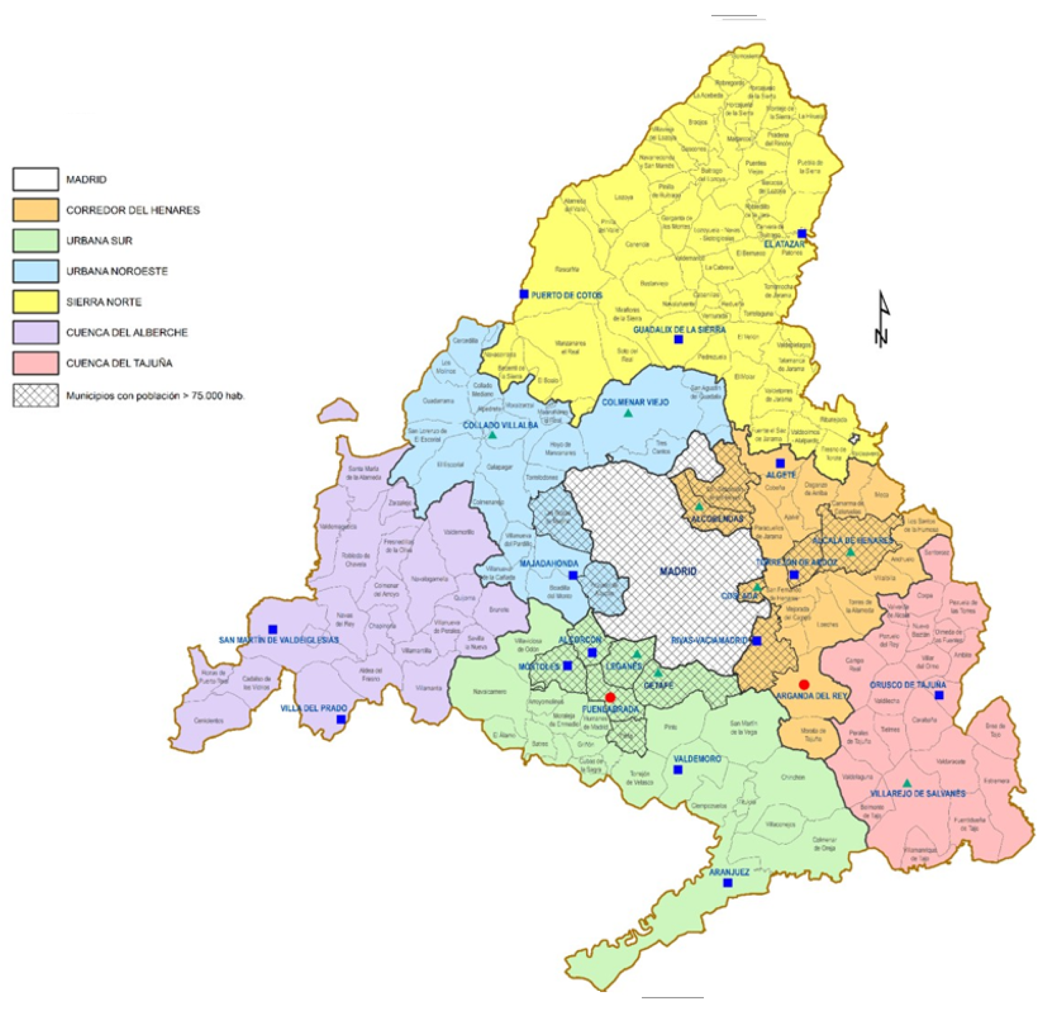
In light of the above arguments, it can be seen why this article has a double objective: first, the estimation of a spatial (panel data) STIRPAT model, where the spatial units are both very small and also highly autonomous and developed municipalities; and second, to examine whether an EKC relationship exists between gross disposable income and NO_x concentrations in the air. For this purpose, a case study has been carried out in the municipalities that make up the Autonomous Community of Madrid, Spain, where outdoor NO_x concentrations are still one of the most concerning pollution problems.

In brief, this article contributes to filling the “true local scale” gap in the literature by exploring the issue of spatial autocorrelation inherent in air pollution at short-to-medium distances within the STIRPAT framework and at a local scale.

It is reasonable to assume that there is spatial dependence in both pollution concentrations and also in most of the drivers of transport-related emissions and other economic forces that cross municipality borders, which may create spatial spillovers. Consequently, we use a spatial Durbin panel data STIRPAT model to account for and estimate such spatial dependencies. Moreover, for comparison purposes, we analyze this spatial dependence by specifying a spatial lag panel data STIRPAT model and a spatial error panel data STIRPAT specification.

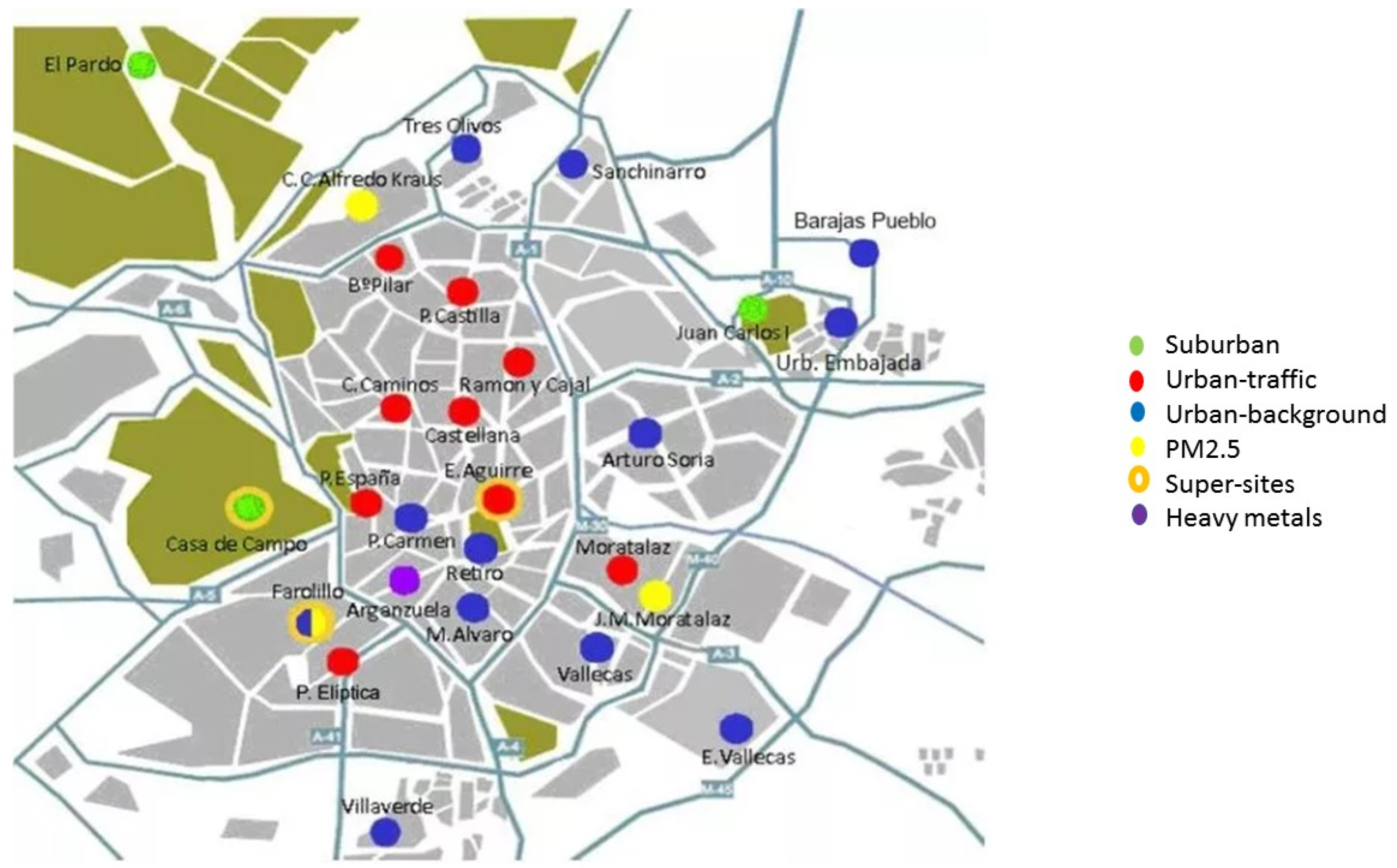
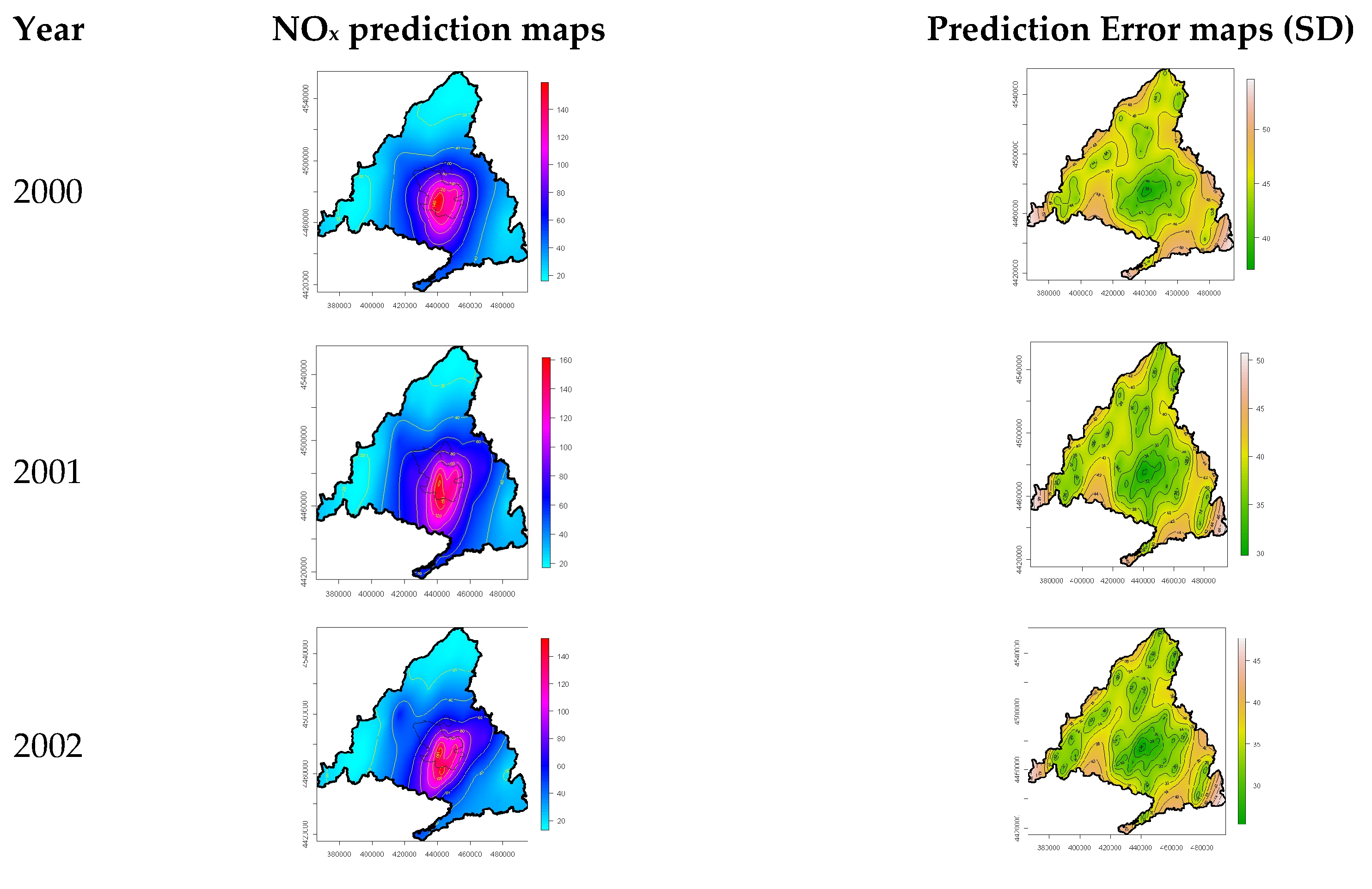
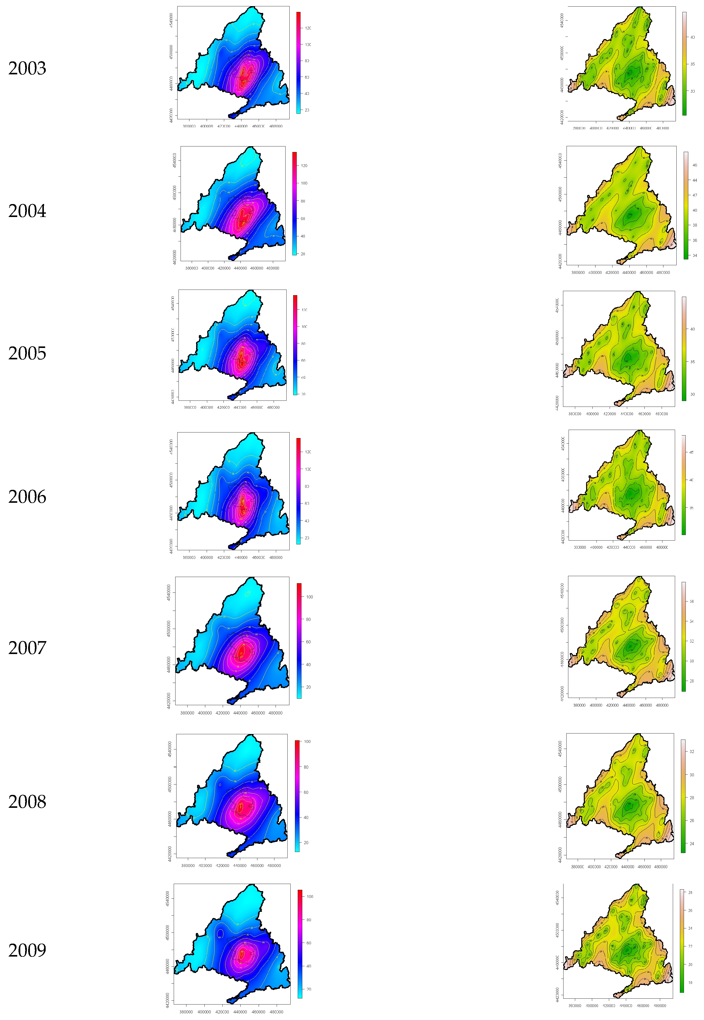
Our analysis focuses on the municipalities that make up the region of Madrid, over the period 2000–2009. The reasons behind the selection of this period are explained in Section 2. It is worth noting that only the highly populated municipalities of the Community of Madrid are equipped with one or more MS. In order to overcome the lack of disaggregated pollution data in the municipalities that are not equipped with MS, we use spatio-temporal kriging, which accounts for spatio-temporal dependencies and enables us to estimate the level of NO_x in the municipalities with no MS.

The remainder of the paper is structured as follows. Section 2 provides a description of the data and methods while Section 3 reports the empirical results. In Section 4 some conclusions are drawn.

2. Data and Methods

2.1. Data

Our analysis is based on the 179 municipalities of the Community of Madrid over the period 2000–2009. There are several reasons behind the selection of this period. The first is that it is the same as the period analyzed in Laureti et al. [8], which allows for the comparison of aspatial and spatial STIRPAT models. The second and more important one is that traffic emissions are considered as the main source of air pollution in the Community of Madrid (especially NO_x concentrations); therefore, the fleet of vehicles per capita is assumed to be the most relevant explanatory variable in the analysis. However, technical advances in fuel efficiency are continuously being incorporated in private vehicles and, fortunately, ever greater reductions in emissions are being achieved. Given this fact, we need information about the “equivalent” fleet of private vehicles, that is, a series of data where the number of cars for year t is expressed in terms of the number of cars of a base year that generate the same amount of pollution. This difficult task was done in Laureti et al. [8] for the period 2000–2009, and we take advantage of this. (iii) The third reason is that in 2010 the Atmosphere Pollution Monitoring System (APMS) of the city of Madrid (the most important municipality of the Community of Madrid; 25 of the 48 MS operating in the Community of Madrid are located in the city of Madrid) was reorganized. The number of MS was substantially reduced and ecologist associations suspected that the municipality of Madrid removed stations from the sites that were potentially the most polluted (Montero and Fernández-Avilés [35]) to manipulate the data. While we could have taken on the task of updating the “equivalent” fleet of private vehicles per capita (a real challenge), we decided against it because of the smaller number of MS after the APMS reorganization and the doubts about the optimality of their location expressed by ecologists associations, which might substantially affect the accuracy of the response variable data.

2.1.1. Dependent Variable

This paper uses the annual mean of NO_x concentration levels as the response variable for a panel of 179 municipalities in the period 2000–2009. The location of the 48 operating MS located across the region of Madrid can be seen in Figure 1. For ease of visualization, we separately depict in Figure 2 the 25 MS operating in the city of Madrid.

As can be seen in Figure 1 and Figure 2, there are different types of MS (traffic, industrial, and background) depending on their location and the impact (or absence) of nearby emissions (pollutant-specific in 2011/850/EU). They also show the type of area, which refers to the environment on a scale of several kilometers. More specifically, the region of Madrid includes three urban areas (Corredor del Henares, Urbana Sur and Urbana Noroeste), three rural areas (Cuenca del Tajuña, Cuenca del Alberche and Sierra Norte) and a seventh zone managed by the City of Madrid Council, which has its own air quality monitoring network. In the city of Madrid, which is divided into five zones (inner M-30, northwest, northeast, southwest, southeast) the APMS is made up of 24 MS. Half of them are background urban, and they are representative of the exposure of the urban population in general. Nine are near traffic, and are located such that their level of pollution is mainly influenced by emissions from a nearby street or road (but it is necessary to avoid measuring very small micro-environments in their vicinity). And three are suburban, located on the outskirts of the city, in places where the highest levels of ozone are found. Background urban and traffic MS are aimed at the protection of human health, while the suburban ones monitor pollution to protect human health and vegetation.

In the rest of the municipalities of the region, in the zoning for NO_x, eight out of the 24 stations of the network are traffic-related, two industrial and 14 background.

It is of note that 155 municipalities out of the total of 179 are not equipped with an air pollution MS. In other words, there are no data on NO_x, the response variable of the STIRPAT approach, for the aforementioned 155 municipalities in the period 2000–2009. Consequently, it is necessary to estimate the value of NO_x in these municipalities. This could be seen as an insurmountable problem; however, as pointed out in Laureti et al. [8], the solution lies in the fact that air pollution data exhibit spatio-temporal dependence (Fernández-Avilés et al. [36]; Montero-Lorenzo et al. [37]), not just spatial dependencies (as mentioned in Laureti et al. [8]). Based on the registers of the existing MS, we used (i) spatio-temporal kriging of the mean (STKotM) for 2000 to 2009, to predict the response value in the period under study in the municipality of Madrid, which was the only municipality with more than one MS, and (ii) spatio-temporal ordinary kriging (STOK) to predict this value in the non-MS-equipped municipalities.

Although both interpolation procedures will be detailed in the methodological section of the paper,

Table 1. Evolution of the mean level of NOx (µg/m³) in the municipalities of the Community of Madrid (grouped by population size, 2000–2009).

Population	N° Mun *	2000	2001	2002	2003	2004	2005	2006	2007	2008	2009
Less than 5000	101	31.96	35.02	29.34	33.71	36.12	36.12	31.04	27.92	30.09	27.43
5000–50,000	58	31.06	34.81	31.12	32.45	35.35	32.14	29.99	26.29	30.16	27.96
50,000–100,000	10	32.99	33.19	39.01	32.65	35.91	40.25	37.04	33.01	29.76	29.55
100,000–250,000	9	68.45	85.04	83.23	86.49	92.15	91.00	80.43	64.88	62.00	54.69
City of Madrid	1	146.24	140.36	121.08	94.33	102.14	98.92	89.07	87.84	76.91	72.48
C. of Madrid	179	97.62	99.11	90.16	77.21	83.12	78.49	71.41	66.62	62.76	56.92

* N° Mun: number of municipalities.

shows the NO_x mean value (registered or estimated by kriging) for municipality clusters based on their population size (thus ensuring the reader is provided with the information while keeping the Table manageable).

As shown in Table 1, the average level of NO_x concentrations in the city of Madrid (72.48 µg/m³ in 2009), although displaying a marked downward trend overall, indicates that the legal standard for health protection (40 µg/m³, annual mean) was clearly exceeded at many of the MS located in the city. The same can be said for the industrial municipalities located in the Southern and Eastern Metropolitan area (most of them in the group with 100,000–250,000 inhabitants). However, in the municipalities with fewer than 100,000 inhabitants (most of them located in wealthy, verdant, nicely urbanized municipalities, close to the mountains, in the Northern and Western Metropolitan area and on the outskirts of Madrid) the annual mean level of NO_x was much lower (slightly below 30 µg/m³), and only exceeded the legal standard in some specific municipalities in 2002 and 2005.

2.1.2. Independent Variables

The factors that potentially influence NO_x concentrations are introduced as explanatory variables. Data for the 179 municipalities over the period 2000–2009 were taken from the ALMUDENA database of the Statistics Office of the Community of Madrid (See http://www.madrid.org/desvan/Inicio.icm?enlace=almudena accessed on 15 February 2021). Considering the specific situation in the Community of Madrid, we carried out the corresponding decomposition and improvements on the population (P) and technology (T) variables in order to understand which are the most important drivers affecting NO_x emissions at a municipality scale, taking into account the geographical distribution of the driving forces in the Community of Madrid.

Bearing in mind the availability of data at municipality level, we specified Population (P) by considering total population, the proportion of the male population between 25 and 55 years of age, and the share of population over 65. Indeed, the environmental pressures of the population can vary among different age groups, which can reflect their degree of independence and potential contribution to economic activity (Liddle [38]; O’Neil et al. [39]). One would expect the economically active part of the population aged 14–64 to have a higher impact on emissions than pensioners over 65 or the age group encompassing children and adolescents under 14 (Cole and Neumayer [40]). However, York [41]) stated that there are reasons to expect that populations with a high proportion of elderly people consume more energy than those composed of younger people. For example, older populations tend to have smaller households and consume more energy intensive products, such as cars. Okada [42] found an inverted U-shaped relationship between CO₂ emissions per capita and the share of people over 65 years old in 25 OECD countries, which are mostly European countries.

The affluence variable (A), which indicates the level of prosperity of each municipality, is described through the gross disposable income (GDI) per capita at 1992 constant prices, electric power consumption (KWh per capita), and value added by the industrial sector (% of GDP). With the aim of testing the EKC hypothesis, the squared term of GDI per capita is also included to capture the possible nonlinear relationship between NO_x concentrations and income. The presence of an EKC is indicated by a negative and significant coefficient for the quadratic term together with a positive and significant coefficient for GDI.

In the STIRPAT literature, the technology variable has been very difficult to define and convert into operational measures. We thus decompose it into various separate factors which influence environmental impacts, such as vehicle fleet, public transport infrastructure and services (number of lines of public transportation, number of train stations, number of bus stops and number of taxis).

The private vehicle population has increased dramatically in many municipalities in recent years. Indeed, the number of vehicles in Madrid has increased by 25.2% between 2000 and 2009, amounting to a total of 4,293,542 in 2009 (5,072,299 in 2019, the last data available), according to the Statistical Yearbook of the Community of Madrid 1985–2019. This translates into 535.2 vehicles per sq.km and 673 vehicles per 1000 inhabitants (761.2 in 2019). In 2009 there were 7,960,000 motorized trips every working day, 46% by public transport and 54% by car (49% and 51%, respectively, in 2019). Technological improvements in the fuel efficiency of new cars was considered by expressing the number of vehicles in terms of equivalent vehicles, thus obtaining the equivalent fleet over the period 2000–2009 where the number of cars for year t is expressed in terms of the number of cars from 2001 that generate the same amount of pollution (Laureti et al. [8]).

Since the regional government has not paid enough attention to the main source of emissions of this dangerous pollutant, the effect of the environmental plans implemented in recent years has been partially offset by the increasing use of road transport. As a result, the number of vehicles may have considerable impact on municipalities’ NO_x concentrations.

On the other hand, an increase in air pollutant emissions is explained not only by the growth of transport activity but also by the shift of transport to more energy-intensive modes and the increase in air pollutant emissions of modes in use. Therefore, in addition to the number of vehicles, the number of lines of public transportation, the number of train stations and the number of bus stops are considered to explain the environmental pressure caused by transportation (Dargay and Gately [43]; Eom and Schipper [44]).

Table 2. Basic summary statistics for quantitative non-location-related covariates (n = 1790).

Quantitative Non-Location Related Covariates	Mean	CV	Min	Max
Population (POP)	32,592.93	7.13	21	3,255,944
Share of population over 65 years (POP65+)	0.16	0.66	0.007	1.193
Share of the male population between ages 25–55 (MALE25-55)	0.30	2.07	0.033	9.022
Value added by industrial sector (INDUSTR)	30.33	0.49	0.010	78.830
GDI per capita at 1992 constant prices (GDI)	8709.25	0.25	4735.912	19,171.580
Electric power consumption (KWh per capita) (ENERGY)	5008.19	0.93	370.370	63,021.300
Equivalent fleet per capita (FLEET)	0.54	1.27	0.016	12.638
Number of heavy vehicles per capita (HEAVY)	120.88	5.67	1	13,087.000
Total number of lines of public transportation per capita (PUBLIC)	0.00	2.02	0.000	0.097
Number of bus stops per capita (BUSSTOP)	0.01	1.47	1	0.163
Number of taxis that travel by highway per capita (TAXI)	0.99	1.52	0.024	24.390

lists the descriptive statistics of the explanatory variables analyzed as potential drivers of outdoor concentrations of NO_x.

Our database also contains a number of time-independent regressors, including membership of the Spanish Network of Cities for the Climate, which coordinates the actions carried out by the various administrations to tackle climate change; the transformation of landfills to green areas, which is aimed at mitigating unhealthy sources of contamination and the proliferation of infestations, in order to minimize the environmental impact on the surrounding area and to create new green zones; and others related to location (longitude, latitude, altitude, extension, distance to the city of Madrid, etc.). However, in order to not make Table 2 unnecessarily long, and because their impacts on the response variable cannot be estimated under fixed effects, they are not listed.

2.2. Methods

2.2.1. Spatio-Temporal Kriging

Kriging is a univariate procedure (which can be extended to cokriging, the multivariate version) which interpolates the values of the target variable at unobserved locations using the available observations of the same variable. This interpolation procedure, which is a minimum mean-squared-error method of spatial prediction, produces the best linear unbiased predictor. For this purpose, kriging uses the covariance or variogram function, which is the spatial (or spatio-temporal) equivalent of the autocorrelation function in time-series analysis. The kriging strategy is based on the idea that variables follow a stochastic process over space or space-time. Other interpolation alternatives have been considered in the literature, such as Thiessen polygons, inverse distance method, splines, etc. However, kriging is more appropriate when dealing with environmental variables (Anselin and Le Gallo [45]) because it considers the spatial or spatio-temporal dependencies and provides a measure for the goodness of the prediction.

In our case, the spatio-temporal framework of an air pollution monitoring situation, let $\left\{Z\left(s_1,t_1\right),\hspace{0.17em}\dots ,Z\left(s_n,t_n\right)\right\}$ be the values of NO_x observed at a set of n spatio-temporal sites $\left\{\left(s_1,t_1\right),\hspace{0.17em}\dots ,\left(s_n,t_n\right)\right\}$ equipped with an air pollution MS across a specific geographical area (in our case, the Community of Madrid). The philosophy of the spatio-temporal geostatistics paradigm when it comes to predicting the concentrations of NO_x in a particular location that is not equipped with an MS at a specific instant of time, $Z\left(s_0,t_0\right)$, or across an area of interest (municipality, province, region, country) has the same logic as that used by economic agents. An economic agent would observe the concentrations at similar spatio-temporal points around $\left(s_0,t_0\right)$ and, more than likely, the prediction provided would be the mean of the observed concentrations. This procedure has an overwhelming logic; the only criticism we can make is that the weight assigned to the concentrations recorded at the sites similar to $\left(s_0,t_0\right)$ should not be the same. This is why the spatio-temporal predictor provided by geostatistics, the so-called spatio-temporal kriging (STK) predictor, is:

$$Z^{*}\left(s_0,t_0\right)={\displaystyle \sum _{i=1}^n{\lambda }_i}Z\left(s_i,t_i\right)$$

(1)

where the weights, ${\lambda }_i$, are obtained so that the resulting predictor is optimal, in the sense of unbiasedness and minimal variance of the prediction error; and this in a framework of non-independence of the variables representing the NO_x concentrations at sites $\left\{\left(s_1,t_1\right),\hspace{0.17em}\dots ,\left(s_n,t_n\right)\right\}$, because the spatio-temporal dependence of air pollutant concentrations is already considered a stylized fact of air pollution data. The resulting STK equations depend on the degree of stationarity attributed to the random function that supposedly generates the observed realization. In the case of second-order or intrinsic stationarity, the usual case, the STK equations are as follows:

$$\{\begin{array}{l}{\displaystyle \sum _{j=1}^n{\lambda }_j\gamma }\left(s_i-s_j,t_i-t_j\right)+\alpha =\gamma \left(s_i-s_0,t_i-t_0\right),\hspace{1em}\forall i=1,\dots ,n\\ {\displaystyle \sum _{j=1}^n{\lambda }_j=1}\end{array}$$

(2)

with prediction (kriging) variance:

$$V\left(Z^{*}\left(s_0,t_0\right)-Z\left(s_0,t_0\right)\right)={\displaystyle \sum _{i=1}^n{\lambda }_i\gamma \left(s_i-s_0,t_i-t_0\right)+\alpha }$$

(3)

where $\gamma \left(s_i-s_j,t_i-t_j\right)$ is the semivariogram selected to capture the structure of the spatio-temporal dependencies existing in the phenomenon under study (in the second-order case, the covariogram $C\left(s_i-s_j,t_i-t_j\right)$ can also be used) and $\alpha$ is a Lagrange multiplier associated with the non-bias condition (see Sherman [46]; Montero et al. [47], for details). In the stationary case—which is our case and the typical case in air pollution databases—the STK procedure detailed above is known as “ordinary” (spatio-temporal ordinary kriging, STOK). In the case of non-stationarity, the corresponding STK procedure is known as “universal” (spatio-temporal universal kriging, STUK). STUK equations for the non-stationary case can also be seen in Montero et al. [47].

The following points should be noted. First, as in the spatial-only case, STK strongly depends on the choice of the autocovariance or semivariogram associated with the space-time random field under study. This is not a problem in spatial-only geostatistics. It could be said that there is a “standard” list of semivariograms that guarantee positive definiteness, covering almost all practical situations. However, in the spatio-temporal context defining such a list is a challenge, because the construction of non-separable spatio-temporal covariance or semivariogram structures (the space-time interaction is crucial for prediction) associated with stationary or non-stationary, isotropic or anisotropic random fields, which meet the requirements to be a valid covariance or semivariogram model, is not an easy task (it is not easy to prove the positive definiteness of a spatio-temporal dependence structure). Even the construction and visualization of an empirical space-time semivariogram can often be considered a challenging task (see example 6.2 in Montero et al. [47]). The original separable, isotropic and stationary covariance models (the metric model by Dimitrakopoulos and Luo [48]; the sum model introduced by Rouhani and Hall [49]; the product model by Rodriguez-Iturbe and Mejia [50], and De Cesare et al. [51]; the product-sum model popularized by De Iaco et al. [52,53]; and the integrated product and product-sum models also popularized by De Iaco et al. [54], among other initiatives) imply a number of restrictive conditions that makes them infeasible options for use in real applications. Therefore, more complex and realistic covariance models were needed to improve predictive performance. Thus, over the past decade a great effort has been made to deal with separability, stationarity, isotropy and full symmetry in the spatio-temporal structures capturing the spatio-temporal dependencies existing in the phenomena under study. Examples of such efforts include the models proposed by Cressie and Huang [55], Gneiting [56], Ma [57,58,59,60], Stein [61] and Porcu and Mateu [62] to take into account the space-time interaction; the specifications by Ma [63] and Gneiting et al. [64] to overcome full symmetry; the mixture-based Bernstein zonally anisotropic covariance functions by Porcu et al. [65] and the non-separable models constructed by using quasi-arithmetic functionals (Porcu et al. [66], which go beyond isotropy; and the non-stationary models developed by Fuentes and Smith [67], Chen et al. [68], Ma [57,69] and Porcu and Mateu [62], among others.

Given the long list of “recent” models cited above, one might think that, as in the spatial-only case, there is a “standard” list of permissible models; however, this is currently far from being the case. The new families of space-time covariance models are not exempt from problems and, in practice, the selection of one of them to represent the space-time dependencies existing in the phenomenon under study continues to be a challenge. Given the complexity of these “new” models, their visualization is recommended, as well as an analysis of how they evolve when the model parameters change; this is core information in the selection of the appropriate model to capture the spatio-temporal dependencies. However, visualization is not easy either, and constitutes another of the pending questions regarding spatio-temporal covariogram analysis (see Montero and Fernández-Avilés [70] for details and advances). By way of example, Huang and Sun [71] state that “it is challenging to visualize and assess separability and full symmetry from spatio-temporal observations”.

As highlighted by Wikle [72] in his book review of Montero et al. [47], “to date, there are no general spatio-temporal covariance or semivariogram models that can adequately describe the complex dynamics that are exhibited by the multivariate, often nonlinear, spatio-temporal processes that govern most real-world processes”.

Second, although it does not apply in our case, when dealing with spatio-temporal data, the solution of STK equations can involve considerable computational burden which might lead to failure in the prediction procedure. More specifically, the calculation of the inverse of covariance matrices becomes a crucial problem. This is known as the “big n problem” (Banerjee et al. [73]), which often arises when dealing with massive spatio-temporal datasets. Accordingly, recent literature emphasizes the use of approximation methods and new methodologies for dealing with massive spatio-temporal data sets.

Third, in case studies and practical applications, it has been found that STK prediction exhibits a very rapid reversion to the mean in locations near the border of the spatial region and/or close to the end of the time period considered (and, of course, in out-of-sample prediction).

2.2.2. Spatio-Temporal Kriging of the Mean

In geostatistics, the problem of estimating the mean value of a variable of interest in a specific area is called the kriging of the mean (KotM). We aim to estimate the unknown mean (in our case for NO_x concentrations in the city of Madrid), in the years under study, ${\mu }_t, t=2000, \dots ,2009$, using the estimator:

$${\mu }^{*}={\displaystyle \sum _{i=1}^n{\lambda }_i}Z\left(s_i,t_i\right)$$

(4)

The weights ${\lambda }_{it}$ are obtained so that the kriging prediction of the mean is unbiased and the prediction error variance is minimal. In order to ensure the unbiasedness of the kriging predictor, the sum of the weights must be one, as $E\left({\mu }_t^{*}-{\mu }_t\right)=\mu {\displaystyle \sum _{i=1}^n{\lambda }_i-}\mu$. The resulting spatio-temporal equations, in terms of a permissible spatio-temporal covariance function are:

$$\{\begin{array}{l}{\displaystyle \sum _{j=1}^n{\lambda }_j}C\left(s_i-s_j,t_i-t_j\right)-\alpha =0,\hspace{1em}\forall i=1,\dots ,n\\ {\displaystyle \sum _{j=1}^n{\lambda }_j=1}\end{array}$$

(5)

which in the stationary case only depends on the distance between the spatio-temporal points. The estimation variance coincides with the Lagrange multiplier $\alpha$.

It is worth noting that in some ways the KotM is the same as the “change of support problem” (COSP). Kriging is very often the solution to overcome this mismatch of spatial support (Gotway and Young [74]), particularly when dealing with socio-economic data (Census data, pollutant concentrations, housing prices, etc.) since it takes into account spatial or spatio-temporal dependencies. When dealing with air pollution data, the usual solution to the abovementioned problem is to krige the environmental variable(s) to obtain their interpolated values in the locations where socio-economic data are available. Two kriging alternatives can be used: (i) the only-spatial KotM for every instant of time considered in the database, which means the estimation of a semivariogram for each instant of time; or (ii) the STKotM, where only one spatio-temporal semivariogram needs to be estimated and used whatever the period for which the mean is estimated. The good performance of STK in the in-sample case (“sandwich predictions”), is the reason why we opt for the second alternative.

2.2.3. A Spatial Formulation of the STIRPAT Model

As stated in Laureti et al. [8], when analyzing environmental pressure, the most widely-used research frameworks addressing different driving forces linking economic features with environmental issues, are the STIRPAT model (York et al. [75]) and the EKC approach (Andreoni and Levinson [76]). We also refer to Laureti et al. [8] and the literature therein, for a review of the literature on the STIRPAT approach to the study of the drivers of environmental impacts.

According to Dietz and Rosa [77,78] the basic version of the STIRPAT model, which evaluates various theoretical frameworks on the systemic drivers of environmental change, is given by:

$$I_i={\beta }_0{P}_i^{{\beta }_1}{A}_i^{{\beta }_2}{T}_i^{{\beta }_3}{e}_i$$

(6)

where I represents the environmental impact, P is population, A is consumption per capita (or affluence), T is technology (or impact per unit of consumption), e is the residual or error term and the subscript i denotes cross-sectional units. ${\beta }_0$, ${\beta }_1$, ${\beta }_2$ and ${\beta }_3$ are the model coefficients or elasticities.

The STIRPAT methodology has mainly been applied at a large scale, using cross-sectional and panel national-level data (see Liddle [79], for a review until 2013; and other papers published in the last five years, such as Wang et al. [80], Al-Mulali et al. [81], Abdallh and Abugamos [82], Koçak and Ulucak [83], Lohwasse et al. [84], and Velez-Henao et al. [85] and the references therein for an updated review).

In the last decade, the STIRPAT approach has also been applied at a “local” scale (county, city and province level). Yin et al. [86], Xu and Lin [87] and Xu et al. [88] in China; Squalli [89]; Roberts [90] in the USA; Scholz [91] in Japan; and Anser [92] in Pakistan are some examples. However, only Laureti et al. [8], in the Community of Madrid, Spain, is an application of STIRPAT at genuinely local scale.

In recent years, the spatial argument has started to play a key role in the framework of environmental changes (see Atwi et al. [9] for a review of the literature for and against controlling for spatial effects in environmental equations). The reasons behind this are the ever-growing popularity of the new developments in spatial econometrics and the awareness that the environment and many of its explanatory factors have a clear spatial nature. However, much of this literature focuses on the EKC hypothesis. Some examples include Rupasingha et al. [21], which estimated Bayesian Tobit SE models to determine the drivers of toxic pollutants in US counties, while Maddison [22] used a panel of SO₂, NO_x, CO and volatile organic compounds emissions in 135 countries to explore different spatial econometric techniques in estimating EKCs. According to Maddison [22], in EKCs, spatial relationships arise most obviously as a consequence of countries’ strategic response to transboundary pollution flows. However, the analysis is a country-level analysis and the two spatial models used (the spatial lag model and the spatial error model) lose much of their utility. Something similar can be said of Poon et al. [93] for SO₂ in China, and for Burnett et al. [94] in the USA, at a state scale, for the period 1970–2009, when analyzing the relationship between CO₂ emissions, energy consumption, economic activity, and pollution emissions while controlling for potential spatial effects within the data, in a panel data framework. At any rate, all of these studies conclude that the EKC equation should control for spatial impacts.

Wang et al. [23] used a spatial econometric approach (spatial lag, spatial error and Durbin models) and found evidence supporting an inverted U-shape EKC between economic growth and ecological footprint.

Pattison et al. [31], in an exploratory study at county level in the USA for the year 2002, and using a spatial regression analysis, tested the hypotheses that affluence is positively related to carbon emissions from consumption activities but negatively related to emissions from production activities.

Zhao et al. [24] used spatial panel data models to investigate the factors influencing energy-related CO₂ emission intensity among a panel of 30 provinces in China covering the period 1991–2010. Hao and Liu [26] analyzed the socio-economic factors influencing urban PM_2.5 concentrations in 73 Chinese cities in 2013 by using Spatial Lag and Spatial Error (SL and SE, respectively) models. Kang et al. [25] examined the CO₂ EKC hypothesis using a spatial panel data model covering the period 1997–2012 for 30 Chinese provinces to avoid the coefficient estimation error. Atwi et al. [9] studied the case of CO₂, by comparing the estimates derived from the cross-sectional and the panel data approaches, with data from 182 countries during the period 1992–2011. They found that the EKC hypothesis is acceptable under both approaches, although the estimated turning points in cross-sections seem unreliable.

Ding et al. [95] examined the existence of EKC for PM_2.5 pollution in the Beijing-Tianjin-Hebei region of China. They utilized satellite observations of PM_2.5 and panel data of 13 cities from 1998 to 2016 to investigate the relationship between economic growth and PM_2.5 pollution. Having tested the existence of spatial effects, a Spatial Durbin (SD) model was chosen for the above purpose although SL and SE were also estimated. Huang et al. [96], Yu et al. [97] and Feng et al. [98], among many others, conducted similar research.

In the light of the above literature, it is clear that research using STIRPAT models and the EKC equation has evolved by including the corresponding terms to control for spatial effects, as their existence has been sufficiently proved in the literature.

As can be noted, most of the literature using the STIRPAT approach accounting for spatial effects relies on US counties and Chinese cities or provinces as spatial support. It is true that this spatial support can be considered “local” compared with countries. However, most counties in the USA (and, of course, cities or provinces in China) cover more area than the most important cities in Europe. As such, spatial dependencies make more sense when dealing with “municipalities” in Europe than when working with counties, cities or provinces as spatial units in the USA or China. By way of example, the average area of a US county is 2911.4 km², the average area of a Chinese province is 291,406 km² and the average area of a municipality in Madrid, the region under study in this article, is 45.36 km². In addition, when considering spatial effects in the estimation of the impacts of a number of covariates on the environment, and especially on air pollution, the population density and the distribution of that population across the spatial unit considered is a key factor; the higher the population density and the more uniformly it is distributed across the territory, the more important it is to consider spatial effects in the STIRPAT model. This is the rationale behind conducting the analysis at a genuinely local scale and carrying out our practical study in a territory in Europe.

We want to make it clear that in local STIRPAT modeling, when dealing with air pollution concentrations, spatial dependencies must be taken into account because in reality a large percentage of local spatial units are not MS-equipped. Consequently, in our case study, where spatial units are the municipalities of the Autonomous Community of Madrid (clearly local units), we are forced to specify a spatial STIRPAT specification because the dependent variable is an interpolated variable (in the sites where pollution concentrations cannot be measured).

Spatial relationships can be modeled in a variety of ways depending on the relationship between the dependent variable and the explanatory variables. Following LeSage and Pace [99], we consider three spatial panel data models; namely, the spatial autoregressive panel data (SL-PD) model, the spatial Durbin panel data (SD-PD) model and the spatial error panel data (SE-PD) model. They allow us to examine three different types of interaction effects among municipalities (geographical units), that is, endogenous interaction effects among the response variable (Y), exogenous interaction effects among the independent variables (X), and interaction effects among the error terms (${\epsilon }_{it}$).

The SL-PD model hypothesizes that the value of the dependent variable observed at a particular location is partially determined by a spatially weighted average of neighboring dependent variables (the first way of specifying interaction between spatial units). That is, NO_x emissions in municipality i are affected by the NO_x emissions in municipality j.

The SL-PD model is expressed as:

$$y_{it}=\alpha i_n+\rho {\displaystyle \sum _{j=1}^N{w}_{ij}}{y}_{jt}+x_{it}^{}\beta +{\zeta }_t+u_i+{\epsilon }_{it}$$

(7)

where $y_{it}$ denotes the dependent variable, I_it, (NO_x emissions) for unit i at time t. $i_n$ is a (n x1) unit vector for the intercept (we have opted to remove the unitary column from $X$ to avoid problems of exact multicollinearity in the estimation process of models including spatially lagged covariates), ρ denotes a scalar spatial autocorrelation coefficient on the dependent variables. The term ${\displaystyle \sum _{j=1}^N{w}_{ij}}{y}_{jt}$ denotes the interaction effect of the dependent variable $y_{it}$ with the dependent variables $y_{it}$ in neighboring municipalities, where $w_{ij}$ is the ij-th element of a pre-specified nonnegative spatial weighting matrix W of order N² describing the spatial arrangement of the units in the sample. ${\zeta }_t$ captures the time-period effects, $u_i$ captures all time-constant unobserved municipality-specific factors, such as the concern of the population regarding the quality of the environment, which could be viewed as being roughly constant over the period in question. ${\epsilon }_{it}$ is the disturbance term, which is i.i.d. across i and t with zero mean and variance σ², both in fixed and random effects models (see for example, Baltagi and Liu [100]).

In the SD-PD strategy, the dependent variable can be predicted as a function of spatially lagged values of the explanatory variables as well:

$$y_{it}=\rho {\displaystyle \sum _{j=1}^N{w}_{ij}}{y}_{jt}+\alpha i_n+x_{it}^{}\beta +{\displaystyle \sum _{j=1}^N{w}_{ij}}{x}_{ijt}^{}\theta +{\zeta }_t+u_i+{\epsilon }_{it}$$

(8)

where θ is a (K × 1) vector of spatial autocorrelation coefficients on the lagged explanatory variables.

If a spatial process of the disturbance (error) term is specified (the second way of specifying the interaction between spatial units), the resulting specification is an SE-PD model, which refers to a situation in which the unobserved shock to municipality i is affected by unobserved shocks in neighboring municipalities:

$$y_{it}=\alpha i_n+x_{it}^{}\beta +{\zeta }_t+u_i+{\varphi }_{it}\hspace{1em}\mathrm{with}\hspace{1em}{\varphi }_{it}=\lambda {\displaystyle \sum _{j=1}^N{w}_{ij}}{\varphi }_{it}+{\epsilon }_{it}$$

(9)

where ${\varphi }_{it}$ reflects the spatially autocorrelated error term and λ is called the spatial autocorrelation coefficient.

It should be noted that: (i) both SL-PD and SE-PD models are nested in the SD-PD model; and (ii) that there are spatial specifications more general than the SD-PD model, such as the spatial Cliff–Ord type autoregressive panel data model, also known as the spatial autoregressive panel data model with Autoregressive Disturbances (SARAR-PD model), which was introduced by Kelejian and Prucha [101]. However, the present study focuses on spillovers and, according to LeSage and Page [100], SARAR-PD specifications concentrate on a more elaborate model for disturbances. In addition, SL-PD and SD-PD strategies, which are nested in SARAR-PD models, provide consistent estimates for the majority of spatially correlated data-generating processes (Minguez et al. [102]).

By referring to a panel data context, and expressing Equation (6) in logarithms so that it becomes additive, the specific a-spatial panel data STIRPAT (PD-STIRPAT) model including the specific response and covariates described in Section 2, can be specified as:

$$\begin{array}{l}\ln NO{x}_{it}={\alpha }_{}+{\beta }_1\ln \left(PO{P}_{it}\right)+{\beta }_2\ln \left(MALE25-{55}_{it}\right)+{\beta }_3\ln \left(POP65{+}_{it}\right)+{\beta }_4\ln \left(GD{I}_{it}\right)\\ +{\beta }_5{\left(\ln \left(GD{I}_{it}\right)\right)}^2+{\beta }_6\ln \left(INDUST{R}_{it}\right)+{\beta }_7\ln \left(ENERG{Y}_{it}\right)+{\beta }_8\ln \left(FLEE{T}_{it}\right)\\ +{\beta }_9\ln \left(HEAV{Y}_{it}\right)+{\beta }_{10}\ln \left(PUBLI{C}_{it}\right)+{\beta }_{11}\ln \left(BUSSTO{P}_{it}\right)+{\beta }_{12}\ln \left(TAX{I}_{it}\right)\\ +{\beta }_{13}PERIO{D}_t+u_i+{\epsilon }_{it}\end{array}$$

(10)

where the subscripts i and t denote municipalities and years, respectively. As mentioned previously, ${\epsilon }_{it}$ is the disturbance term, $u_i$ captures all time-constant unobserved municipality-specific factors, such as the concern of the population regarding the quality of the environment, which could be viewed as being roughly constant over the period in question.

As outlined above, an additional term $\rho {\displaystyle \sum _{j=1}^N{w}_{ij}}{y}_{jt}$ leads to the SL-PD- STIRPAT specification (with $\rho$ being the spatial autoregressive coefficient); and another additional term ${\displaystyle \sum _{j=1}^N{w}_{ij}}{x}_{ijt}^{}\theta$ leads to the SD-PD-STIRPAT model. However, the inclusion of the spatially autocorrelated error term ${\varphi }_{it}=\lambda {\displaystyle \sum _{j=1}^N{w}_{ij}}{\varphi }_{it}+{\epsilon }_{it}$ would specify the SE-PD-STIRPAT strategy.

It is important to note that in SL- and SD-PD-STIRPAT models, the spatial impacts are not given directly by any vector of parameters. However, the expressions of direct and indirect effects, as well as of the averaged direct, indirect, and total impacts can be seen in

Table 3. Total, direct, and indirect impacts on the response variable resulting from a change in covariates: Spatial-PD-STIRPAT models.

Model	Direct Impact	Indirect Impact	Total Impact
SL	$\frac{tr\left\{{(I_n-\rho W)}^{-1}{I}_n{\beta }_k\right\}}{n}$	Total-Direct	$\frac{i_n^T\left\{{(I_n-\rho W)}^{-1}{I}_n{\beta }_k\right\}{i}_n}{n}$
SE	${\beta }_K$	$0$	${\beta }_k$
SD	$\frac{tr\left\{{(I_n-\rho W)}^{-1}\left(I_n{\beta }_k+W{\theta }_k\right)\right\}}{n}$	Total-Direct	$\frac{i_n^T\left\{{(I_n-\rho W)}^{-1}\left(I_n{\beta }_k+W{\theta }_k\right)\right\}{i}_n}{n}$

. (LeSage and Page [100]).

With the aim of testing the EKC hypothesis, the squared term of GDI per capita is also included to capture the possible nonlinear relationship between NO_x concentrations and income.

Given that (i) the assumption of zero correlation between the random effects and the explanatory variables is particularly restrictive, and that (ii) in spatial research it is at least controversial that the number of units is potentially able to go to infinity and that the units of observation are representative of a larger population, which are three conditions that should be satisfied before the random effects model can be implemented (Elhorst [103]), we opt for fixed effects modeling. Some researchers implement Lagrange multiplier tests to inform the above decision. However, these tests have proven to have high power for a large number of data-generating processes in the alternative hypothesis (anyway, the spatial extension of the Haussman test (Mutl and Pfaffermayr [104]) indicates that the data do not support the random effects assumption (chi-sq = 649.4, df = 21, p-value < 2.2 × 10⁻¹⁶; chisq = 456.73, df = 21, p-value < 2.2 × 10⁻¹⁶; and chisq = 5311.6, df = 23, p-value < 2.2 × 10⁻¹⁶ for the SL-, SE- and SE-PD-STIRPAT models, respectively).

The decision to estimate fixed effects models implies that some location-related covariates cannot be included in the model because they are time-invariant.

As for which lagged drivers of NO_x to include in the SD-PD-STIRPAT model, the corresponding nested likelihood ratio tests were implemented.

The estimation method used was Maximum Likelihood. Two-Stage Least Squares estimation could have been implemented if it were suspected that some of the regressors were endogenous, but that is not the case in our study. Therefore, there was no need to use instrumental variables.

Finally, all computations were conducted using the libraries splm (Millo and Piras [105]), spdep (Bivand and Piras [106]) and maptools (Bivand and Lewin-Koh, [107]) in R (R Development Core Team [108]).

3. Results

3.1. Spatio-Temporal Kriging Results for NO_x Predicted Values

Figure 3 shows both the NO_x spatio-temporal prediction maps and prediction errors maps for the 179 municipalities of the Autonomous Community of Madrid, years 2000–2009. Table 1 in Section 2.1 summarizes the main descriptive statistics of their values. The spatio-temporal covariance function used in the prediction process, both in the STK and STKotM equations, was the non-separable spatio-temporal covariance function proposed in Gneiting [56]:

$$C(h,\tau ,\theta )=\frac{{\sigma }^2}{\left(a{\tau }^{2\alpha }+1\right)}\exp \left(\frac{-c{h}^{2\delta }}{{\left(a{\tau }^{2\alpha }+1\right)}^{\beta \delta }}\right),\hspace{1em}\left(h,\tau \right)\in {ℝ}^d\times ℝ$$

(11)

where $a$ and $c$ are two positive space and time scale parameters, respectively, and ${\sigma }^2$ is the a priori variance of the NO_x stochastic process; $\delta$ and $\alpha$ are the space and time smoothing parameters, respectively, with values in the interval (0, 1]; and $\beta$ is the space-time interaction parameter, which moves in the interval [0, 1]. The larger the $\beta$, the more intense the spatio-temporal dependence degree in the stochastic process under study. $h$ and $\tau$ are the spatial distance and the time lag, respectively, and $\theta$ represents the set of parameters involved in the covariance function.

The reasons behind this decision are (i) the shape of the NO_x empirical spatio-temporal covariogram; (ii) it is a non-separable function; (iii) it is sufficiently general for use with air pollution concentrations series.

Table 4. Moran’s I statistics for the logs of NO_x.

Year	Estimate	Year	Estimate
2001	0.7987	2006	0.8031	Expectation	−0.0056
2002	0.8091	2007	0.7824	Variance	0.0023
2003	0.8073	2008	0.7940	p-value	<2.2 × 10−16
2004	0.7959	2009	0.8083
2005	0.7826

lists the values of Moran’s I for the period under study, which confirm the existence of spatial autocorrelation in NO_x concentrations also from a spatial econometrics perspective.

3.2. Coefficients, Direct Impacts and Spillovers

The first finding obtained from the results commented in Section 3.1 and those listed in

Table 5. Estimates of the spatial autocorrelation parameters for a-spatial and spatial-PD-STIRPAT models.

	SL	SE	SD
RHO	0.0530 [0.0320] *	NA	0.0395 [0.0223] *
LAMBDA	NA	0.0442 [0.0378]	NA
W*PUBLIC	NA	NA	−0.1443 [0.0276] ***
W*BUSSTOP	NA	NA	−0.0962 [0.0448] **

*, **, ***: significant at the 10%, 5% and 1% significance level, respectively.

is that space matters and that the model used to specify the spatial PD-STIRPAT representation of the NO_x concentrations in the Autonomous Community of Madrid is far from irrelevant. Our results indicate that, although the spatial correlation coefficient in the SE-PD-STIRPAT model, λ, is not significant, space matters. This is shown by the fact that (i) in the SL- and SD-PD STIRPAT models ρ has a significant value (at the 10% level), although it is very moderate; and (ii) some lagged explanatory factors such as W*PUBLIC and W*BUSSTOP show significant (and notable) spatial autocorrelation coefficients at the 1% and 5% level of significance, respectively. It is no surprise that λ is not significant, because the set of factors we have used as explanatory variables is among the best used in the literature. Consequently, as advanced in the introductory section, an SD-PD-STIRPAT model at local scale, which takes into account the effects of spatial dependencies inherent in air pollution concentrations and some of the factors that cause them, is a perfect candidate for estimating the stochastic impacts on NO_x of Population, Affluence, and Technology in the Autonomous Community of Madrid.

Further exploring spatial effects, the individual effects, which allow for the inclusion of a certain degree of time-invariant unobserved spatial heterogeneity in the model, are shown in Figure 4. Since they capture some idiosyncratic characteristics of the municipalities (including the time-invariant variables longitude, latitude, altitude, extension, distance to the city center, etc.), whose impacts on the response variable are beyond doubt but cannot be estimated when dealing with fixed effects estimation, they might account for some part of the autocorrelation effects.

The first finding detailed above (an SD-PD-STIRPAT model at local scale is a perfect candidate to estimate the stochastic impacts of P, A and T on NO_x) is consistent with the second one: the SD-PD-STIRPAT model is the spatial specification that best captures and fits the spatial dependence within the relationship between transport-related NO_x concentrations and socio-economic drivers at municipal level, where the relationship between socio-economic factors and the environment becomes more complex. As can be seen in

Table 6. Goodness-of-fit measures for a-spatial and spatial-PD-STIRPAT models.

	A-Spatial	SL	SE	SD
R squared	0.65715	0.6815	0.6620	0.6978
LogLikelihood	−1519.6142	−1335.0431	−1422.926	−1196.2410
AIC	3083.2284	2714.0872	2891.8520	2440.4828
BIC	3024.0078	2834.8663	3018.1213	2572.2415

, the three competing spatial panel data models provide similar results for fixed effects estimation. According to the Akaike and Bayesian Information criteria (AIC and BIC, respectively), the best model is SD-PD-STIRPAT. In addition, the LR test-statistic (277.6051, df = 2, p-value < 2.2 × 10⁻¹⁶) to test whether the SD-PD-STIRPAT model can be simplified to SL-PD-STIRPAT has been rejected. It is also observed that the R² of the spatial-PD-STIRPAT strategies is slightly larger than the R² of the a-spatial one. This is an expected result because, as stated in Elhorst ([109], p. 9), “researchers frequently find a weak evidence in favor of the spatial interaction effects when the fixed time effects are considered in the model”.

Finally, the last reason to select the SD-PD-STIRPAT model is that the focus of the article is on both local and global effects.

Third, as can be seen in

Table 7. Estimates of total impacts: a-spatial model and spatial-PD-STIRPAT models.

COVARIATES	A-Spatial	SL	SE	SD
POP	0.2602 [0.0615] ***	−0.0114 [0.0160]	−0.0092 [0.0150]	−0.0118 [0.0162]
POP65+	0.0597 [0.0348] ***	−0.1612 [0.0403] ***	−0.1460 [0.0320] **	−0.0992 [0.0403] **
MALE25-65	0.2412 [0.0591] ***	−0.0159 [0.0378]	−0.0112 [0.0372]	−0.0010 [0.0405]
GDI	0.5767 [2.5263]	−14.3100 [4.3378] ***	−12.8450 [3.7076] ***	−10.0240 [4.2482] **
GDI (SQUARED)	−0.0409 [0.1415]	0.7668 [0.2374] ***	0.6871 [0.2024] ***	0.5363 [0.2322] **
INDUST	0.0028 [0.0085	−0.0258 [0.0127] *	−0.0197 [0.0118] *	−0.0216 [0.0118] *
ENERGY	0.0570 [0.0153] ***	0.1423 [0.0261] ***	0.1267 [0.0254] ***	0.1223 [0.0266] ***
FLEET	0.2000 [0.0503] ***	0.0868 [0.0289] ***	0.0596 [0.0272] **	0.0644 [0.0300] ***
PUBLIC	−0.0365 [0.0117] **	−0.1747 [0.0232] ***	−0.1671 [0.0218] ***	−0.1393 [0.0218] ***
BUSSTOP	0.0283 [0.0121] **	0.0432 [0.0191] **	0.0492 [0.0208] **	0.0270 [0.0217]
TAXI	−0.0172 [0.0072] **	0.0454 [0.0214] **	−0.0461 [0.0200] **	0.0298 [0.0198] *
HEAVY	0.0065 [0.0072]	0.0943 [0.0074] ***	0.0870 [0.0067] ***	0.0846 [0.0075] ***
year_2001	0.1393 [0.0119] ***	0.1550 [0.0571] ***	0.1473 [0.0512] ***	0.1524 [0.0524] ***
year_2002	−0.0349 [0.0129] ***	−0.0295 [0.0534]	−0.0309 [0.0515]	−0.0504 [0.0561]
year_2003	0.0520 [0.0139] **	0.0661 [0.0572]	0.0593 [0.0518]	0.0312 [0.0542]
year_2004	0.1541 [0.0153] ***	0.1832 [0.0611] ***	0.1686 [0.0527] ***	0.1256 [0.0560] **
year_2005	0.1315 [0.0183] ***	0.1468 [0.0603] ***	0.1329 [0.0539] **	0.0837 [0.0634]
year_2006	−0.0489 [0.0200] *	−0.0400 [0.0567]	−0.0467 [0.0545]	−0.1047 [0.0608]
year_2007	−0.2389 [0.0231] ***	−0.2591 [0.0613] ***	−0.2562 [0.0558] ***	−0.3276 [0.0613] *
year_2008	−0.1227 [0.0234] ***	−0.1473 [0.0625] **	−0.1509 [0.0564] ***	−0.2148 [0.0602] ***
year_2009	−0.2135 [0.0256] ***	−0.2296 [0.0657] ***	−0.2297 [0.0580] ***	−0.3096 [0.0596] ***
WX
W*PUBLIC	NA	NA	NA	−0.1501 [0.0274] ***
W*BUSSTOP	NA	NA	NA	−0.1001 [0.0473] **

Standard error in brackets. *, **, ***: significant at the 10%, 5% and 1% significance level, respectively.

, only one of the three covariates representing “Population”, POP65+, has significant stochastic impacts on the level of NO_x concentrations in the region of Madrid, at the significance level of 1% in the SL model and 5% in the SD strategy. The negative relationship of this Population covariate with NO_x concentrations is an expected result, because in the Autonomous Community of Madrid, like in the other Spanish Autonomous Communities, the population living in municipalities in the countryside (also called “empty Spain”) or near to the mountain is the oldest. The “empty Spain” factor also explains why in the a-spatial PD-STIRPAT model both POP and MALE25-65 are highly significant.

As for the covariates representing “Affluence”, which indicates the level of prosperity of each municipality, all of them significantly impact NO_x air pollution. The variables showing the greatest (negative) impact on NO_x are GDI and ENERGY. However, as expected in a region like Madrid—where the richest municipalities are residential municipalities located in the northern and western part of the region, near to the mountains and plenty of pleasant green areas, and the industrial ones are in south and east, where land is cheaper—GDI has a negative impact whereas the impact of ENERGY is positive. This finding is reinforced by the fact that the impact of INDUST on NO_x concentrations is positive and significant at the 10% level of significance. It is of note that only ENERGY is significant when spatial dependencies are not considered in the panel data model; in addition its impact on NO_x is less than half the impact estimated when space is included in the PD-STIRPAT strategy.

Finally, regarding “Technology”, all the covariates included under this element turned out to be significant (with the exception of BUSSTOP in the SD model). The one with the greatest (negative) impact is the total number of lines of public transportation per capita (PUBLIC), regardless of the spatial model used. The second-ranking covariate is HEAVY, with a positive impact, as expected. Third is FLEET, with similar positive impacts to HEAVY. It is worth noting that in the a-spatial PD-STIRPAT model, the most influential covariate is FLEET, whereas HEAVY has the least impact. BUSSTOP and TAXI have similar impacts on the level of NO_x concentrations, although, evidently, with opposite sign. Surprisingly, in the SE model, TAXI has a negative sign.

Time effects are mostly significant and notable, and in line with the evolution of the air pollutant under study over the time period analyzed. Interestingly, there are no singular differences between the estimates provided by the a-spatial and the spatial PD-STIRPAT strategy.

Given the moderate values of the rho coefficient in both SL- and SD-PD-STIRPAT models, the total effects are mostly direct effects (

Table 8. Indirect Impacts: SL- and SD- PD-STIRPAT model.

COVARIATES	SL	SD
POP	−0.0005	−0.0005
POP65+	−0.0084	−0.0089
MALE25-65	−0.0008	−0.0001
GDI	−0.7511	−0.3890
GDI (SQUARED)	0.0402	0.0408
INDUST	−0.0013	−0.0004
ENERGY	0.0074	0.0097
FLEET	0.0046	0.0010
PUBLIC	−0.0092	−0.0084
BUSSTOP	0.0022	0.0011
TAXI	0.0024	0.0011
HEAVY	0.0049	0.0033
year_2001	0.0081	0.0059
year_2002	−0.0015	−0.0019
year_2003	0.0034	0.0012
year_2004	0.0096	0.0049
year_2005	0.0077	0.0032
year_2006	−0.0021	−0.0041
year_2007	−0.0136	−0.0127
year_2008	−0.0077	−0.0083
year_2009	−0.0121	−0.0120

Shaded cells in the indirect impacts indicate significance at the 10% significance level. Direct effects can be obtained by subtracting the indirect effects from the total ones. The level of significance for direct effects is the same as for total effects (Table 7).

). However, POP65+, GDI, ENERGY and PUBLIC indirect effects or spillovers are significant in both SL- and SD- PD-STIRPAT models. FLEET and HEAVY indirect effects are significant in the SL model, and the two lagged variables, W*PUBLIC and W*BUSSTOP, indirectly influence NO_x concentrations in the SD strategy. Consequently, a change in the previous non-lagged and lagged covariates in a particular municipality has an average cumulative effect on the corresponding variables in neighboring municipalities.

Table A1. Estimates of coefficients for Spatial-PD-STIRPAT models (Fixed Effects).

COVARIATES	SL	SE	SD
POP	−0.0108 [0.0156]	−0.0092 [0.0150]	−0.0114 [0.0156]
POP65+	−0.1526 [0.0386] ***	−0.1460 [0.0320] **	−0.0953 [0.0388] **
MALE25-65	−0.0151 [0.0390] ***	−0.0112 [0.0372]	−0.0010 [0.0389]
INCOME	−13.5515 [3.8173] ***	−12.8450 [3.7076] ***	−9.6325 [3.6170] ***
GDI (SQUARED)	0.7262 [0.2085] ***	0.6871 [0.2024] ***	0.5154 [0.2084] **
INDUST	−0.0244 [0.0120] **	−0.0197 [0.0118] *	−0.0208 [0.0119] *
ENERGY	0.1347 [0.0259] ***	0.1267 [0.0254] ***	0.1176 [0.0259] ***
FLEET	0.0822 [0.0277] ***	0.0596 [0.0272] **	0.06353 [0.0280] ***
PUBLIC	−0.1675 [0.0226] ***	−0.1671 [0.0218] ***	−0.1339 [0.0227] ***
BUSSTOP	0.0419 [0.0212] **	0.0492 [0.0208] **	0.0259 [0.0216]
TAXI	0.0430 [0.0208] **	−0.0461 [0.0200] **	0.0279 [0.0209]
HEAVY	0.0893 [0.0068] ***	0.0870 [0.0067] ***	0.0813 [0.0069] ***
2001	0.0361 [0.0087] ***
2002	−0.0179 [0.0094] **
2003	0.0119 [0.0100]
2004	0.0424 [0.0110] ***
2005	0.0313 [0.0129] **
2006	−0.0183 [0.0140]
007	−0.0705 [0.0160] ***
008	−0.0390 [0.0164] **
009	−0.0688 [0.0178] ***
WX
*PUBLIC	NA	NA	−0.1443 [0.0276] ***
*BUSSTOP	NA	NA	−0.0962 [0.0448] **

Standard error in brackets. *, **, ***: significant at the 10%, 5% and 1% significance level, respectively.

in the Appendix A lists the coefficients for the a-spatial and spatial PD-STIRPAT models considered in our analysis.

Table A2. Estimates of the spatial autocorrelation parameters for spatial-PD-STIRPAT models.

	SL	SE	SD
RHO	0.7164 [0.0000] ***	NA	0.7045 [0.0000] ***
LAMBDA	NA	0.7269 [0.0000] ***	NA
W*PUBLIC	NA	NA	−0.0608 [0.0146] ***
W*BUSSTOP	NA	NA	0.0419 [0.0169] **

**, ***: significant at the 5% and 1% significance level, respectively.

,

Table A3. Estimates of coefficients for Spatial-PD-STIRPAT models (Random Effects).

COVARIATES	SL	SE	SD
POP	0.0148 [0.0132]	0.0026 [0.0129]	0.0134 [0.0133]
POP65+	−0.0050 [0.0223]	−0.0159 [0.0221]	0.0029 [0.0229]
MALE25-65	0.0676 [0.0363] **	0.0385 [0.0337]	0.0690 [0.0363] **
INCOME	0.5959 [1.6798]	0.7971 [1.5907]	0.5906 [1.6767]
GDI (SQUARED)	−0.0381 [0.0935]	−0.0481 [0.0887]	−0.0367 [0.0933]
INDUST	0.0026 [0.0060]	0.0026 [0.0056]	0.0025 [0.0060]
ENERGY	0.0269 [0.0110] **	0.0122 [0.0104]	0.0239 [0.0110] **
FLEET	0.0262 [0.0185]	0.0211 [0.0178]	0.0219 [0.0185]
PUBLIC	−0.0169 [0.0085] **	−0.0068 [0.0081]	−0.0163 [0.0084] **
BUSSTOP	−0.0009 [0.0087]	−0.0071 [0.0084]	−0.0007 [0.0087]
TAXI	−0.0161 [0.0053] ***	−0.0157 [0.0049] ***	−0.0163 [0.0053] ***
HEAVY	0.0077 [0.0049]	0.0040 [0.0048]	0.0081 [0.0049]
2001	0.0361 [0.0087] ***	0.1366 [0.0316] ***	0.0377 [0.0087] ***
2002	−0.0179 [0.0094] *	−0.0601 [0.0318]	−0.0211 [0.0094] **
2003	0.0119 [0.0101]	0.0569 [0.0319]	0.0073 [0.0101]
2004	0.0424 [0.0110] ***	0.1610 [0.0322] ***	0.0438 [0.0112] ***
2005	0.0313 [0.0129] **	0.1206 [0.0328] ***	0.0311 [0.0131] **
2006	−0.0183 [0.014]	−0.0611 [0.0332] **	−0.0236 [0.0142] *
2007	−0.0705 [0.0160] ***	−0.2452 [0.0341] ***	−0.0819 [0.0161] ***
2008	−0.0390 [0.0164] **	−0.1175 [0.034] ***	−0.0460 [0.0165] ***
2009	−0.0688 [0.0178] ***	−0.2306 [0.0349] ***	−0.0768 [0.0179] ***
WX
W*PUBLIC	NA	NA	−0.0609 [0.0146] ***
W*BUSSTOP	NA	NA	0.0419 [0.0169] **

*, **, ***: significant at the 10%, 5% and 1% significance level, respectively.

and

Table A4. Indirect Impacts: SL- and SD- PD-STIRPAT model (Random Effects).

COVARIATES	SL	SD
POP	0.0347	0.0298
POP65+	−0.0119	0.1531
MALE25-65	0.1589 *	0.0065 **
INCOME	1.3999	1.3096
GDI (SQUARED)	−0.0894	−0.0814
INDUST	0.0061	0.0056
ENERGY	0.0631 **	0.0532 **
FLEET	0.0616	0.0486
PUBLIC	−0.0397 **	−0.0362 **
BUSSTOP	−0.0022	−0.0017
TAXI	−0.0378 ***	−0.0362 ***
HEAVY	0.0182	0.0179 *
year_2001	0.0848	0.08361 ***
year_2002	−0.0421 *	−0.0468 **
year_2003	0.0279	0.0161
year_2004	0.0997 ***	0.0972 ***
year_2005	0.0736 **	0.0690 **
year_2006	−0.0429	−0.0524 *
year_2007	−0.1656 ***	−0.1815 ***
year_2008	−0.0917 **	−0.1021 ***
year_2009	−0.1616 ***	−0.1704 ***
WX
W*PUBLIC	NA	−0.1350 ***
W*BUSSTOP	NA	0.0930 **

*, **, ***: significant at the 10%, 5% and 1% significance level, respectively. Direct effects can be obtained subtracting the indirect effects from the total ones. The level of significance for direct effects is the same as for total effects (Table A3).

show the results obtained when estimating an RE model.

3.3. Testing the EKC

As can be seen in Table 6, GDI displays a negative sign and GDI (squared) a positive one, irrespective of the spatial-PD-STIRPAT strategy considered, indicating a U-shaped curve instead of the traditional inverted-U.

The result obtained is not in line with the EKC introduced by Grossman and Krueger [110]; that is, an inverted U-shaped relationship between income and pollutant emissions, which assumes that environmental quality worsens in the early stages of development but improves after a certain level of income is reached (see Tzeremes [111,112] for details). According to the empirical evidence, it is indeed shown that for some high-income economies and for certain pollutants the relationship between per capita income and pollution follows an inverted U shape (Falconi et al. [113]). However, as stated in Falconi et al. [113], it must be taken into account that the shape of EKC depends on the pollutant under analysis, the region and the period being studied (to which we would add the length of the period under study). It has been empirically proven that there is an inverted U-shaped ECK for local pollutants. However, for global pollutants, emissions increase with economic growth. In our case study, our database refers only to the period 2000–2009 and to a specific (small) region of a specific country. Using these data, we find a U-shaped relationship, which is probably the consequence of the environmental measures promoted by the Autonomous Community of Madrid at the turn of this century and the spatial distribution of income across the region. In this respect, it is noteworthy that when spatial dependencies are not considered, the shape of the EKC is the traditional inverted U-shaped. Thus, space and spatial dependencies matter (in this case in the short term, at a local scale) when dealing with the EKC.

3.4. Policy Implications

The above results yield important economic implications, which are of interest to policy-makers. The significance of the spatial autocorrelation coefficient ρ is a finding of vital importance for the success of political decisions on environmental issues. As outlined in the introductory section, the existence of spatial spillovers indicates that the level of NO_x concentrations in a municipality affects and is affected by the level of NO_x in neighboring municipalities, which in turn means that environmental governance of a municipality impacts and is impacted by environmental governance in neighboring municipalities. In addition, the existence of significant and notable spatial effects on NO_x derived from some lagged explanatory covariates or drivers (we are referring to the theta coefficients), indicates to environmental policy-makers in the region of Madrid that NO_x-related policies implemented in a municipality influence the results of policies in neighboring municipalities. From this, we can infer that the various municipalities should work together to balance pro-environmental and economic policy goals. This is especially important in geographical areas composed of highly autonomous spatial units, as is the case of municipalities in the region of Madrid. Therefore, in light of this result, convincing policy makers to act in a coordinated way is of crucial importance. In fact, the lack of coordination among mayors belonging to political parties of different ideologies plays a role in preventing further progress on air pollution control. It is true that, in the period under study, the magnitude of the rho coefficient in the region of Madrid is not very high; however, environmental policy-makers must pay special attention to it because it may increase (or decrease) in a short period of time.

Elaborating on the case of the spatial effects produced by the lagged drivers of NO_x (theta coefficients), the “Total number of lines of public transportation per capita (PUBLIC)” and the “Number of bus stops per capita (BUSSTOP)” are the only covariates producing spatial effects on NO_x derived from their spatial lags in the region of Madrid for the period under study. This suggests that municipal actions aimed at increasing both the number of buses and bus stops contribute to clean air not only in the implementing municipality but also in the neighboring municipalities. Consequently, in the presence of this type of effect, municipal actions aimed at improving air quality are not only the concern of the municipality that carries them out, but are also a matter of solidarity with neighboring municipalities. This applies especially in the case of the number of bus stops per capita, because its total impact on NO_x is not significant for the non-lagged variable, but is for its lagged version.

The above results stand in contrast to the fact that none of the private sector-related covariates has significant lagged effects on the NO_x concentrations of neighboring municipalities, which reinforces the need for cooperation at a municipal level in public transportation activities. Undoubtedly, this municipal cooperation will be of great help in significantly reducing the concentrations levels of the only air pollutant still out of control in some areas of the region of Madrid.

An additional effort must be made to reduce the negative impact of some technology-related drivers of NO_x in the region of Madrid. We are referring to the “equivalent fleet of private vehicles per capita” and the “number of heavy vehicles per capita”. Both have a positive and significant impact on the level of NO_x concentrations. As such, it is our opinion that efforts should be made to promote green driving in general and electric vehicles in particular. Electric vehicles are expected to significantly reduce road transport emissions, given an increasingly renewable power generation. While outstanding technological issues are continually being solved, the economic viability of a greener driving is still constrained by the large gap currently existing between conventional and green vehicles. Consequently, municipalities should strive to democratize green driving by promoting green transport technology (especially for electric vehicles), subsidizing their purchase and facilitating charging options (especially for private households), while promoting other clean transportation alternatives (especially in urban environments). This is a good moment for the municipal authorities of the region of Madrid (and also for regional and state authorities) to put the above measures into action, because they could play a key role in tackling the crisis currently afflicting the automotive sector in particular, and the economic crisis in general. It is more than likely that, in the future, when conventional vehicles have been replaced by electrical and other green vehicles, the covariate “vehicles fleet” will no longer impact the level of NOx concentrations.

As for EKC-related recommendations to municipal policy makers of the region of Madrid, again, spatial effects matter and the shape of the NO_x concentrations-income relationship in Madrid is an issue of concern for all the municipalities. Accordingly, they should all collaborate in addressing it to achieve the desired shape.

Finally, in the current framework in which both the private and public sectors strongly support compliance with the principles of Environmental, Social, and Corporate Governance (ESG), having information on the direct and indirect effects of the main drivers of NO_x pollution on the magnitude of its concentrations greatly facilitates governance oriented towards balancing economic activity and clean air. We entirely agree with Uchiyama [114] and Ozcan et al. [115] that the path towards sustainable development can be suggested as optimal policy for (in our case) municipalities, emphasizing the coexistence rather the trade-off between economic growth and the environment. Therefore, the main target of the policies associated with the path of sustainable growth is the creation of a working framework unifying economic development and the environment.

In brief, the spatial panel data Durbin STIRPAT model we contribute for estimating the direct and indirect impacts on NO_x concentrations of its main drivers in the region of Madrid, at a municipal level, constitutes a valuable instrument for policy making oriented towards controlling this dangerous pollutant. Perhaps the main lesson to be learned from the estimates obtained is that reducing NO_x concentrations is a collaborative task, because environmental measures taken by a municipality of the region affect the concentration levels of the pollutant in neighboring municipalities.

4. Conclusions

In recent decades, the STIRPAT framework has been widely adopted to explore the environment-development nexus at macro level, involving cross-national data, and to a lesser extent at local scale, finding evidence on the way that different socio-economic factors including population, income and technology influence air pollution concentrations. However, the majority of researchers have addressed this relevant research question (i) without considering the spatial dependencies existing in air pollution concentrations and also in the drivers of said concentrations, and (ii) based on large spatial units due to the difficulties in finding data on the drivers of air pollution concentrations at a true local level. These two facts may well be core issues when it comes to explaining the lack of robust results to date.

The first main conclusion obtained in this article is that space matters; consequently, we observe a significant change in the estimates of the impact of the drivers of NO_x concentrations on the level of such concentrations when the spatial dependencies in both NO_x and some of its drivers are considered in the STIRPAT model. In addition, the decomposition of the total impacts into direct and indirect (spillovers) impacts is of vital importance for policy makers. This is especially true in the region of Madrid, where the level of NO_x concentrations in a few areas remains a pending air pollution issue. Knowledge about the magnitude of such impacts is core information for the environmental decision-makers to determine the magnitude of the environmental measures to be taken, while also ensuring the objectives are achieved not only in their own municipality, province, etc., but also in the neighboring municipalities, provinces, etc. Indeed, as this study has shown, their decisions on NO_x pollution drivers also affect other neighboring areas; and vice versa—NO_x concentration levels of an area are affected by decisions taken by the policy-makers of neighboring areas. More specifically, knowing the size of the spillovers allows for joint agreements and policies with neighboring areas (municipalities in the case of the region of Madrid) to export the benefits of environmental measures taken in an area (municipality) to neighboring areas (municipalities) and limit negative externalities. Therefore, the existence of significant spatial dependencies in air pollution concentrations suggests we should put an end to autonomous governance of this environmental issue and move towards collaborative governance.

The second main conclusion is that the spatial STIRPAT models used to estimate the relationship of population, income and technology with air pollution concentrations and the magnitude of their impacts (direct and indirect) must be estimated at a local scale. The reason reflects Tobler’s first law of geography (“everything is related to everything else, but near things are more related than distant things”), which, according to the literature on air pollution, applies in the field of atmospheric pollution. In addition, Tobler’s postulate has been supported by the vast literature on the topic using spatial statistics, especially geostatistics and spatial econometrics. However, the range of significant spatial dependencies, which can be estimated with a semivariogram, rarely exceeds a few kilometers, suggesting that spatial STIRPAT models should not be estimated for large spatial units (regions, countries, etc.). Obviously, this calls into question the results obtained from the literature estimating STIRPAT models at a large scale.

More specifically, in this article we have estimated (using fixed effects estimation given the nature of the problem under study) the a-spatial Durbin panel data STIRPAT model together with the spatial lag, error and Durbin panel data STIRPAT models. As noted above, the main conclusion drawn in this article is that space matters when estimating the stochastic impacts of Population, Affluence, and Technology on NO_x in the municipalities of the Autonomous Community of Madrid. Accordingly, the models used to estimate such relationships must be able to capture the spatial dependencies existing in both the response variable and some of the covariates. In line with theoretical premises, the spatial panel data STIRPAT strategy that best captures and represents the spatial dependencies in the NO_x concentrations and the drivers of these concentration levels in the region of Madrid is the Durbin model. We cannot state that we contribute a new spatial STIRPAT econometric model capably of capturing spatial dependencies, because the panel data version of the spatial lag, spatial error or spatial Durbin STIRPAT models have been already used in the literature. However, in this article, we contribute to filling the “true local scale” gap in the literature by exploring the issue of spatial autocorrelation inherent in air pollution at short-to-medium distances within the STIRPAT framework and at a local scale.

Dealing with data at a local scale usually involves a lack of information, especially when using air pollution variables as response variables, because there are fairly few atmospheric pollution MS, even in very big cities. In this article we have solved this problem using spatio-temporal kriging techniques, which provide very high-quality estimates. In addition, in spite of the limitations in obtaining information on the drivers of NO_x at a very local scale, this article contributes one of the best databases (in fact a proprietary database) feeding STIRPAT models with air pollution concentrations in the response variable.

Although space matters, the magnitude of the spatial autocorrelation coefficient is moderate, both in the spatial lag and spatial Durbin strategies, which can be attributed to the fact that some time-invariant covariates representative of the unobserved spatial heterogeneity have not been included in the models given their fixed effects nature.

It has been shown that POP65+, all the “Affluence” variables (GDI, ENERGY and INDUST; especially GDI and ENERGY) and all covariates coming under “Technology” (with the exception of BUSSTOP) have significant impacts (with the expected sign) on the level of NO_x concentrations under an SD structure. These total impacts are mostly direct. In addition, POP65+, GDI, ENERGY and PUBLIC as well as the two lagged variables, W*PUBLIC and W*BUSSTOP, have significant spillovers. In other words, a change in them in a particular municipality has an average cumulative effect on the corresponding variables in neighboring municipalities. Time effects are mostly significant and notable, and in line with the evolution of this air pollutant over the period under study.

In addition, we have included the squared term of GDI in the model in order to test the EKC. Our finding is that when spatial dependencies are not considered, the shape of the EKC is the traditional inverted-U; however, we observe a non-inverted-U when space is accounted for in the model. Thus, space and spatial dependencies matter (in this case in the short term, at a local scale) when dealing with the EKC. Nevertheless, it must be borne in mind that our case study refers to a recent and short period of time in a specific region of a specific country and this finding should be corroborated by further, similar local-scale case studies. In the meantime, we support the statement by Falconi et al. [113]) that the shape of the EKC depends on the pollutant under analysis, the region and the period being studied, especially for short periods of time and at a local scale.

In brief, from a practical perspective, we contribute a spatial panel data Durbin STIRPAT model which can be of great interest for the environmental authorities and policy-makers of the Autonomous Community of Madrid, an important Spanish region with levels of NO_x concentrations which frequently exceed the legal limits, and whose citizens are deeply concerned about the issue of air pollution. As far as we know, this is the first spatial STIRPAT model estimated for the region of Madrid. In addition, we do not know of any other papers using spatial STIRPAT modeling at a similar local scale to the one used in this article. Consequently, we cannot compare the results obtained for the region of Madrid with results obtained for other areas at local scale. An alternative option would be to compare our results with those obtained in studies that estimate spatial STIRPAT models on the basis of large spatial units (provinces in China, counties in the USA, countries, etc.). However, according to Tobler’s law, this comparison makes no sense from a spatial econometric perspective. We strongly encourage other researchers to apply these strategies at a local scale in other regions with high air pollution concentrations, in order to see whether their findings corroborate or contradict our findings.

The spatial panel data Durbin STIRPAT model we contribute, which can be estimated dynamically, is an instrument of particular importance in the current environmental framework shaped by the ESG principles and the United Nations 2030 Agenda, as it greatly facilitates the environmental governance demanded by the citizens of modern societies.

Finally, we would be interested in future theoretical research on semiparametric spatial panel data STIRPAT modeling, especially using penalized splines for smoothing purposes. This approach would not only account for spatial autocorrelation and spatial heterogeneity but also the non-linear (smooth) relationships between certain drivers of the response variable and the response variable. We are also interested in seeing the application of functional data analysis to the detection of air pollution episodes and outliers (see Martinez Torres et al. [116] for a recent application in the city of Dublin, Ireland).

References

1. European Environmental Agency. Environmental Indicators: Typology and Use in Reporting; Internal Working Paper; EEA: Copenhagen, Denmark, 2003. [Google Scholar]
2. EEA. New Initiative to Measure Outdoor Air Quality at Schools Across Europe; European Environment Agency. 2019. Available online: https://www.eea.europa.eu/highlights/new-initiative-to-measure-outdoor (accessed on 24 November 2020).
3. EEA. Air Quality in Europe—2019 Report; EEA Report No 10/2019, European Environment Agency. 2019. Available online: https://www.eea.europa.eu/publications/air-quality-in-europe-2019 (accessed on 20 November 2020).
4. Long-Term Air Quality Trends in Europe—Fine Particulate Matter (PM2.5) Health Impacts. Available online: file:///C:/Users/MDPI/AppData/Local/Temp/ETCACM_TP_2017_4_AQTrendsHIA.pdf (accessed on 20 November 2020).
5. IARC. Outdoor Air Pollution a Leading Environmental Cause of Cancer Deaths; Press Release No 221; International Agency for Research on Cancer. 2013. Available online: http://www.iarc.fr/en/media-centre/iarcnews/pdf/pr221_E.pdf (accessed on 22 November 2020).
6. OECD. The Economic Consequences of Outdoor Air Pollution, OECD Publishing; Paris. 2016. Available online: https://doi.org/10.1787/9789264257474-en (accessed on 20 November 2020).
7. Ecologistas en Acción de Madrid. La Calidad del Aire en la Ciudad de Madrid Durante 2019; Report|9 January 2020. Available online: https://www.ecologistasenaccion.org/wp-content/uploads/2020/01/info-calidad-aire-madrid-2019.pdf (accessed on 16 November 2020). (in Spanish).
8. Laureti, T.; Montero, J.M.; Fernández-Avilés, G. A Local Scale Analysis on Influencing Factors of NOx Emissions: Evidence from the Community of Madrid, Spain. Energy Policy 2014, 74, 557–568. [Google Scholar] [CrossRef]
9. Atwi, M.; Barberán, R.; Mur, J.; Angulo, A. CO2 Kuznets curve revisited: From cross-sections to panel data models. Investig. Reg. J. Reg. Res. 2018, 40, 169–196. [Google Scholar]
10. Elliott, J.R.; Clement, M.T. Developing spatial inequalities in carbon appropriation: A sociological analysis of changing local emissions across the United States. Soc. Sci. Res. 2015, 51, 119–131. [Google Scholar] [CrossRef] [PubMed]
11. Mosconi, E.M.; Colantoni, A.; Gambella, F.; Cudlinová, E.; Salvati, L.; Rodrigo-Comino, J. Revisiting the Environmental Kuznets Curve: The Spatial Interaction between Economy and Territory. Economics 2020, 8, 74. [Google Scholar] [CrossRef]
12. Kairis, O.; Karavitis, C.; Salvati, L.; Kounalaki, A.; Kosmas, K. Exploring the Impact of Overgrazing on Soil Erosion and Land Degradation in a Dry Mediterranean Agro-Forest Landscape (Crete, Greece). Arid Land Res. Manag. 2015, 29, 360–374. [Google Scholar] [CrossRef]
13. Brenner, N. Metropolitan Institutional Reform and the Rescaling of State Space in Contemporary Western Europe. Eur. Urban Reg. Stud. 2003, 10, 297–324. [Google Scholar] [CrossRef]
14. Destek, M.A.; Sarkodie, S.A. Investigation of Environmental Kuznets Curve for Ecological Footprint: The Role of Energy and Financial Development. Sci. Total Environ. 2019, 650, 2483–2489. [Google Scholar] [CrossRef]
15. Destek, M.A.; Ulucak, R.; Dogan, E. Analyzing the Environmental Kuznets Curve for the EU Countries: The Role of Ecological Footprint. Environ. Sci. Pollut. Res. 2018, 25, 29387–29396. [Google Scholar] [CrossRef]
16. Expósito, A.; Pablo-Romero, M.; Sánchez-Braza, A. Testing EKC for Urban Water Use: Empirical Evidence at River Basin Scale from the Guadalquivir River, Spain. J. Water Resour. Plan. Manag. 2019, 145, 04019005. [Google Scholar] [CrossRef]
17. Li, T.; Wang, Y.; Zhao, D. Environmental Kuznets Curve in China: New Evidence from Dynamic Panel Analysis. Energy Policy 2016, 91, 138–147. [Google Scholar] [CrossRef]
18. Lin, B.; Omoju, O.E.; Nwakeze, N.M.; Okonkwo, J.U.; Megbowon, E.T. Is the Environmental Kuznets Curve Hypothesis a Sound Basis for Environmental Policy in Africa? J. Clean. Prod. 2016, 133, 712–724. [Google Scholar] [CrossRef]
19. Gill, A.R.; Viswanathan, K.K.; Hassan, S. Is Environmental Kuznets Curve Still Relevant? Int. J. Energy Econ. Policy 2017, 7, 156–165. [Google Scholar]
20. Luzzati, T.; Orsini, M.; Gucciardi, G. A Multiscale Reassessment of the Environmental Kuznets Curve for Energy and CO2 Emissions. Energy Policy 2018, 122, 612–621. [Google Scholar] [CrossRef]
21. Rupasingha, A.; Goetz, S.J.; Debertin, D.; Pagoulatos, A. The environmental Kuznets curve for US counties: A spatial econometric analysis with extensions. Pap. Reg. Sci. 2004, 83, 407–424. [Google Scholar] [CrossRef]
22. Maddison, D. Environmental Kuznets curves: A spatial econometric approach. J. Environ. Econ. Manag. 2006, 51, 218–230. [Google Scholar] [CrossRef]
23. Wang, Y.; Kang, L.; Wu, X.; Xiao, Y. Estimating the environmental Kuznets curve for ecological footprint at the global level: A spatial econometric approach. Ecol. Indic. 2013, 34, 15–21. [Google Scholar] [CrossRef]
24. Zhao, X.; Burnett, J.W.; Fletcher, J.J. Spatial analysis of China province-level CO2 emission intensity. Renew. Sustain. Energy Rev. 2014, 33, 1–10. [Google Scholar] [CrossRef] [Green Version]
25. Kang, Y.-Q.; Zhao, T.; Yang, Y.-Y. Environmental Kuznets curve for CO2 emissions in China: A spatial panel data approach. Ecol. Indic. 2016, 63, 231–239. [Google Scholar] [CrossRef]
26. Hao, Y.; Liu, Y.-M. The influential factors of urban PM2.5 concentrations in China: A spatial econometric analysis. J. Clean. Prod. 2016, 112, 1443–1453. [Google Scholar] [CrossRef]
27. Hao, Y.; Wu, Y.; Wang, L. Re-examine environmental Kuznets curve in China; Spatial estimations using environmental quality indexes. Sustain. Cities Soc. 2018, 42, 498–511. [Google Scholar] [CrossRef]
28. Zhang, J.; Zhang, K.; Zhao, F. Spatial effects of economic growth, energy consumption and environmental pollution in the provinces of China—An empirical study of a spatial econometrics model. Sustain. Dev. 2020, 28, 868–879. [Google Scholar] [CrossRef]
29. Roberts, T.D. Applying the STIRPAT model in a post-Fordist landscape: Can a traditional econometric model work at the local level? Appl. Geogr. 2011, 31, 731–739. [Google Scholar] [CrossRef]
30. Videras, J. Exploring spatial patterns of carbon emissions in the USA: A geographically weighted regression approach. Popul. Environ. 2014, 36, 137–154. [Google Scholar] [CrossRef]
31. Pattison, A.; Habans, R.C.; Matthew, T. Ecological modernization or aristocratic conservation: Exploring the impact of affluence on emissions. Soc. Nat. Resour. 2014, 27, 850–866. [Google Scholar] [CrossRef]
32. Georgiev, E.; Mihaylov, E. Economic growth and the environment: Reassessing the environmental Kuznets Curve for air pollution emissions in OECD countries. Lett. Spat. Resour. Sci. 2015, 8, 29–47. [Google Scholar] [CrossRef]
33. Çatic, A.N.; Karaçuka, M.; Huyugüzel-Kisla, G. Air Pollution and Income Relationship in Turkish Provinces: A Spatial Approach. Marmara Üniversitesi İktisadi İdari Bilimler Dergisi 2016, 38, 127–146. [Google Scholar] [CrossRef] [Green Version]
34. Sunarni, N. Environmental Kuznets Curve for Environmental Quality in Indonesia: A Spatial Econometric Approach; 201908; Department of Economics; Padjadjaran University. 2019. Available online: https://ideas.repec.org/s/unp/wpaper.html (accessed on 23 October 2020).
35. Montero, J.M.; Fernández-Avilés, G. Functional kriging prediction of atmospheric particulate matter concentrations in Madrid, Spain: Is the new monitoring system masking potential public health problems? J. Clean. Prod. 2018, 175, 283–293. Available online: https://www.sciencedirect.com/science/article/pii/S0959652617329712 (accessed on 2 September 2020). [CrossRef]
36. Fernández-Avilés, G.; Minguez, R.; Montero, J.M. Geostatistical air pollution indices and spatial hedonic and models: The case of Madrid, Spain. J. Real Estate Res. 2012, 342, 243–274. [Google Scholar] [CrossRef]
37. Montero-Lorenzo, J.M.; Fernández-Avilés, G.; Mondéjar-Jiménez, J.; Vargas-Vargas, M. A spatio-temporal geostatistical approach to predicting pollution levels: The case of mono-nitrogen oxides in Madrid. Comput. Environ. Urban. 2013, 37, 95–106. [Google Scholar] [CrossRef]
38. Liddle, B. Demographic dynamics and per capita environmental impact: Using panel regressions and household decompositions to examine population and transport. Popul. Environ. 2004, 261, 23–39. [Google Scholar] [CrossRef]
39. O’Neill, B.C.; Liddle, B.; Jiang, L.; Smith, K.R.; Fuchs, R.; Dalton, M.; Pachauri, S. Demographic change and carbon dioxide emissions. Lancet 2012, 380, 157–164. [Google Scholar] [CrossRef]
40. Cole, M.A.; Neumayer, E. Examining the impact of demographic factors on air pollution. Popul. Environ. 2004, 261, 5–21. [Google Scholar] [CrossRef] [Green Version]
41. York, R. Demographic trends and energy consumption in European Union Nations, 1960–2025. Soc. Sci. Res. 2007, 36, 855–872. [Google Scholar] [CrossRef]
42. Okada, A. Is an increased elderly population related to decreased CO2 emissions from road transportation? Energy Policy 2012, 45, 286–292. [Google Scholar] [CrossRef]
43. Dargay, J.; Gately, D. Vehicle ownership to 2015: Implications for energy use and emissions. Energy Policy 1997, 2514, 1121–1127. [Google Scholar] [CrossRef]
44. Eom, J.; Schipper, L. Trends in passenger transport energy use in South Korea. Energy Policy 2010, 387, 3598–3607. [Google Scholar] [CrossRef]
45. Anselin, L.; Le Gallo, J. Interpolation of Air Quality Measures in Hedonic House Price Models: Spatial Aspects. Spat. Econ. Anal. 2006, 1, 31–52. [Google Scholar] [CrossRef]
46. Sherman, M. Spatial Statistics and Spatio-Temporal Data: Covariance Functions and Directional Properties; John Wiley & Sons: Chichester, UK, 2011. [Google Scholar]
47. Montero, J.M.; Fernández-Avilés, G.; Mateu, J. Spatial and Spatio-Temporal Geostatistical Modeling and Kriging; Wiley Series in Probability and Statistics; John Wiley & Sons: Chichester, UK, 2015. [Google Scholar]
48. Dimitrakopoulos, R.; Luo, X. Spatiotemporal Modeling: Covariances and Ordinary Kriging System. In Geostatistics for the Next Century; Dimitrakopoulos, R., Ed.; Kluwer Academic Publisher: Dordrecht, The Netherlands, 1994; pp. 88–93. [Google Scholar]
49. Rouhani, S.; Hall, T.J. Space-Time Kriging of Groundwater Data. In Geostatistics; Armstrong, M., Ed.; Kluwer Academic Publishers: Dordrecht, The Netherlands, 1989; pp. 639–651. [Google Scholar]
50. Rodríguez-Iturbe, I.; Mejia, J.M. The design of rainfall networks in time and space. Water Resour. Res. 1974, 10, 713–728. [Google Scholar] [CrossRef]
51. De Cesare, L.; Myers, D.; Posa, D. Spatial-Temporal Modeling of SO2 in Milan District. In Geostatistics Wollongong’96; Baafi, E.Y., Schofield, N.A., Eds.; Kluwer Academic Publishers: Dordrecht, The Netherlands, 1997; Volume 2, pp. 1031–1042. [Google Scholar]
52. De Iaco, S.; Myers, D.E.; Posa, D. Space-time analysis using a general product-sum model. Stat. Probab. Lett. 2001, 52, 21–28. [Google Scholar] [CrossRef]
53. De Iaco, S.; Myers, D.E.; Posa, D. Space-time variograms and a functional form for total air pollution measurements. Comput. Stat. Data Anal. 2002, 41, 311–328. [Google Scholar] [CrossRef]
54. De Iaco, S.; Myers, D.E.; Posa, D. Nonseparable space-time covariance models: Some parametric families. Math. Geol. 2002, 34, 23–42. [Google Scholar] [CrossRef]
55. Cressie, N.; Huang, C. Classes of nonseparable, spatiotemporal stationary covariance functions. J. Am. Stat. Assoc. 1999, 94, 1330–1340. [Google Scholar] [CrossRef]
56. Gneiting, T. Nonseparable stationary covariance functions for space-time data. J. Am. Stat. Assoc. 2002, 97, 590–600. [Google Scholar] [CrossRef]
57. Ma, C. Spatio-temporal covariance functions generated by mixtures. Math. Geol. 2002, 34, 965–975. [Google Scholar] [CrossRef]
58. Ma, C. Spatio-temporal stationary covariance models. J. Multivar. Anal. 2003, 86, 97–107. [Google Scholar] [CrossRef] [Green Version]
59. Ma, C. Linear combinations of space-time covariance functions and variograms. IEEE Trans. Signal Process. 2005, 53, 857–864. [Google Scholar]
60. Ma, C. Semiparametric spatio-temporal covariance models with the ARMA temporal margin. Annals Inst. Math. Stat. 2005, 57, 221–233. [Google Scholar] [CrossRef]
61. Stein, M.L. Space-time covariance functions. J. Am. Stat. Assoc. 2005, 100, 310–321. [Google Scholar] [CrossRef]
62. Porcu, E.; Mateu, J. Mixture-based modeling for space-time data. Environmetrics 2007, 18, 285–302. [Google Scholar] [CrossRef]
63. Ma, C. Families of spatio-temporal stationary covariance models. J. Stat. Plan. Inference 2003, 116, 489–501. [Google Scholar] [CrossRef]
64. Gneiting, T.; Genton, M.G.; Guttorp, P. Geostatistical Space-Time Models, Stationarity, Separability and Full Symmetry. In Statistical Methods for Spatio-Temporal Systems; Finkenstadt, B., Held, L., Isham, V., Eds.; Chapman and Hall/CRC: Boca Raton, FL, USA, 2007; pp. 151–175. [Google Scholar]
65. Porcu, E.; Gregori, P.; Mateu, J. Nonseparable stationary anisotropic space–time covariance functions. Stoch. Environ. Res. Risk Assess. 2006, 21, 113–122. [Google Scholar] [CrossRef]
66. Porcu, E.; Mateu, J.; Christakos, G. Quasi-arithmetic means of covariance functions with potential applications to space–time data. J. Multivar. Anal. 2009, 100, 1830–1844. [Google Scholar] [CrossRef] [Green Version]
67. Fuentes, M.; Smith, R. A New Class of Nonstationary Spatial Models. J. Am. Stat. Assoc. 2003, 1–28. [Google Scholar]
68. Chen, L.; Fuentes, M.; Davis, J.M. Spatial temporal statistical modelling and prediction of environmental processes. In Hierarchical Modelling for the Environmental Sciences; Clark, J.S., Gelfand, A., Eds.; Oxford University Press: Oxford, UK, 2006; pp. 121–144. [Google Scholar]
69. Ma, C. Nonstationary covariance functions that model space-time interactions. Stat. Probab. Lett. 2003, 61, 411–419. [Google Scholar] [CrossRef]
70. Montero, J.M.; Fernández-Avilés, G. The role of visualisation in the choice of stationary non-separable space-time covariance functions: An application to air pollution data. Int. J. Geogr. Inf. Sci. 2015, 29, 1887–1909. [Google Scholar] [CrossRef]
71. Huang, H.; Sun, Y. Visualization and Assessment of Spatio-temporal Covariance Properties. Spatial Statistics Visualization and Assessment of Spatio-temporal Covariance Properties. Spat. Stat. 2017, 34. [Google Scholar] [CrossRef] [Green Version]
72. Wikle, C.K. Book Review: José-María Montero, Gema Fernández-Avilés, and Jorge Mateu: Spatial and Spatio-Temporal Geostatistical Modeling and Kriging. J. Agric. Biol. Environ. Stat. 2017, 22, 420–422. [Google Scholar] [CrossRef]
73. Banerjee, S.; Carlin, B.P.; Gelfand, A.E. Hierarchical Modeling and Analysis of Spatial Data; Chapman and Hall/CRC Press: Boca Raton, FL, USA, 2004. [Google Scholar]
74. Gotway, C.A.; Young, L.J. Combining Incompatible Spatial Data. J. Am. Stat. Assoc. 2002, 97, 632–648. [Google Scholar] [CrossRef] [Green Version]
75. York, R.; Rosa, E.A.; Dietz, T. STIRPAT, IPAT and ImPACT: Analytic tools for unpacking the driving forces of environmental impacts. Ecol. Econ. 2003, 46, 351–365. [Google Scholar] [CrossRef]
76. Andreoni, J.; Levinson, A. The simple analytics of the environmental Kuznets curve. J. Public Econ. 2001, 80, 269–286. [Google Scholar] [CrossRef] [Green Version]
77. Dietz, T.; Rosa, E.A. Rethinking the environmental impacts of population, affluence and technology. Hum. Ecol. Rev. 1994, 1, 277–300. [Google Scholar]
78. Dietz, T.; Rosa, E.A. Effects of population and affluence on CO2 emissions. Proc. Natl. Acad. Sci. USA 1997, 94, 175–179. [Google Scholar] [CrossRef] [PubMed] [Green Version]
79. Liddle, B. Impact of population, age structure, and urbanization on carbon emissions/energy consumption: Evidence from macro-level, cross-country analyses. Popul. Environ. 2013. [Google Scholar] [CrossRef] [Green Version]
80. Wang, Y.; Zhang, X.; Kubota, J.; Zhu, X.; Lu, G. A semi-parametric panel data analysis on the urbanization-carbon emissions nexus for OECD countries. Renew. Sustain. Energy Rev. 2015, 48, 704–709. [Google Scholar] [CrossRef]
81. Al-Mulali, U.; Ozturk, I.; Solarina, S.A. Investigating the environmental Kuznets curve hypothesis in seven regions: The role of renewable energy. Ecol. Indic. 2016, 67, 267–282. [Google Scholar] [CrossRef]
82. Abdallh, A.A.; Abugamos, H. A semi-parametric panel data analysis on the urbanisation-carbon emissions nexus for the MENA countries. Renew. Sustain. Energy Rev. 2017, 78, 1350–1356. [Google Scholar] [CrossRef]
83. Koçak, E.; Ulucak, Z.Ş. The effect of energy R&D expenditures on CO2 emission reduction: Estimation of the STIRPAT model for OECD countries. Environ. Sci. Pollut. Res. 2019, 26, 14328–14338. [Google Scholar]
84. Lohwasser, J.; Schaffer, A.; Brieden, A. The role of demographic and economic drivers on the environment in traditional and standardized STIRPAT analysis. Ecol. Econ. 2020, 178, 106811. [Google Scholar] [CrossRef]
85. Velez-Henao, J.-A.; Font Vivanco, D.; Hernández-Riverosa, J.A. Technological change and the rebound effect in the STIRPAT model: A critical view. Energy Policy 2019, 129, 1372–1381. [Google Scholar] [CrossRef]
86. Yin, J.; Zheng, M.; Chen, J. The effects of environmental regulation and technical progress on CO2 Kuznets curve: An evidence from China. Energy Policy 2015, 77, 97–108. [Google Scholar] [CrossRef]
87. Xu, B.; Lin, B. Regional differences of pollution emissions in China: Contributing factors and mitigation strategies. J. Clean. Prod. 2016, 112, 1454–1463. [Google Scholar] [CrossRef]
88. Xu, F.; Huang, Q.; Yue, X.; He, C.; Wang, C.; Zhang, H. Reexamining the relationship between urbanization and pollutant emissions in China based on the STIRPAT model. J. Environ. Manag. 2020, 273, 111134. [Google Scholar] [CrossRef] [PubMed]
89. Squalli, J. An empirical assessment of U.S. state-level immigration and environmental emissions. Ecol. Econ. 2010, 69, 1170–1175. [Google Scholar] [CrossRef]
90. Roberts, T. Integrating economic geography and relative cohort size into a panel interaction model of carbon dioxide emissions in the US, 2000–2009. Popul. Assoc. Am. 2013, 72, 123–139. [Google Scholar]
91. Scholz, S. The POETICS of industrial carbon dioxide emissions in Japan: An urban and institutional extension of the IPAT identity. Carbon Balance Manag. 2006, 1, 36–49. [Google Scholar] [CrossRef] [PubMed] [Green Version]
92. Anser, M.K. Impact of energy consumption and human activities on carbon emissions in Pakistan: Application of STIRPAT model. Environ. Sci. Pollut. Res. 2019, 26, 13453–13463. [Google Scholar] [CrossRef] [PubMed]
93. Poon, J.; Casas, I.; He, C. The impact of energy, transport and trade on air pollution in China. Eurasian Geogr. Econ. 2006, 47, 568–584. [Google Scholar] [CrossRef]
94. Burnett, J.W.; Bergstrom, J.C.; Dorfman, J.H. A spatial panel data approach to estimating US state-level energy emissions. Energy Econ. 2013, 40, 396–404. [Google Scholar] [CrossRef]
95. Ding, Y.; Zhang, M.; Chen, S.; Wang, W.; Nie, R. Environmental Kuznets curve for PM2.5 pollution in Beijing-Tianjin-Hebei region of China: A spatial panel data approach. J. Clean. Prod. 2019, 220, 984–994. [Google Scholar] [CrossRef]
96. Huang, W.; Wang, H.; Zhao, H.; Wei, Y. Temporal-Spatial Characteristics and Key Influencing Factors of PM2.5 Concentrations in China based on STIRPAT Model and Kuznets Curve. 2019. Volume 18, No. 12, 2587–2604. Available online: http://www.eemj.icpm.tuiasi.ro/ (accessed on 1 October 2020).
97. Yu, X.; Wu, Z.; Zheng, H.; Li, M.; Tan, T. How urban agglomeration improve the emission efficiency? A spatial econometric analysis of the Yangtze River Delta urban agglomeration in China. J. Environ. Manag. 2020, 260, 110061. [Google Scholar] [CrossRef]
98. Feng, T.; Du, H.; Lin, Z.; Zuo, J. Spatial spillover effects of environmental regulations on air pollution: Evidence from urban agglomerations in China. J. Environ. Manag. 2020, 272, 110998. [Google Scholar] [CrossRef]
99. LeSage, P.; Pace, R.K. Introduction to Spatial Econometrics; Chapman & Hall/CRC Press: Boca Raton, FL, USA, 2009. [Google Scholar]
100. Baltagi, B.H.; Liu, L. An improved generalized moments estimator for a spatial moving average error model. Econ. Lett. 2011, 113, 282–284. [Google Scholar] [CrossRef]
101. Kelejian, H.H.; Prucha, I. Specification and estimation of spatial autoregressive models with autoregressive and heteroskedastic disturbances. J. Econom. 2010, 157, 53–67. [Google Scholar] [CrossRef] [PubMed] [Green Version]
102. Mínguez, R.; Montero, J.-M.; Fernández-Avilés, G. Measuring the impact of pollution on property prices in Madrid: Objective versus subjective pollution indicators in spatial models. J. Geogr. Syst. 2013, 15, 169–191. [Google Scholar] [CrossRef]
103. Elhorst, J.P. Spatial Econometrics. From Cross-Sectional Data to Spatial Panels; Springer: Berlin/Heidelberg, Germany, 2014. [Google Scholar]
104. Mutl, J.; Pfaffermayr, M. The Haussman test in a Cliff and Ord panel model. Econom. J. 2011, 14, 48–76. [Google Scholar] [CrossRef]
105. Millo, G.; Piras, G. splm: Spatial Panel Data Models in R. J. Stat. Softw. 2012, 47, 1–38. Available online: http://www.jstatsoft.org/v47/i01/ (accessed on 3 October 2020). [CrossRef] [Green Version]
106. Bivand, R.; Piras, G. Comparing Implementations of Estimation Methods for Spatial Econometrics. J. Stat. Softw. 2015, 63, 1–36. Available online: http://www.jstatsoft.org/v63/i18/ (accessed on 21 October 2020). [CrossRef] [Green Version]
107. Bivand, R.; Lewin-Koh, N. Package ‘Maptools’. 2020. Available online: https://cran.r-project.org/web/packages/maptools/maptools.pdf (accessed on 21 October 2020).
108. R Development Core Team. R: A Language and Environment for Statistical Computing. R Foundation for Statistical Computing; R Team: Vienna, Austria, 2020; Available online: https://www.R-project.org/ (accessed on 21 October 2020).
109. Elhorst, J.P. Spatial Panel Data Models. In Handbook of Applied Spatial Analysis: Software Tools, Methods and Applications; Fischer, M.M., Getis, A., Eds.; Springer Science & Business Media: Berlin/Heidelberg, Germany, 2009. [Google Scholar]
110. Grossman, G.; Krueger, A. Environmental Impacts of the North American Free Trade Agreement—NBER; Working Paper 3914; National Bureau of Economic Research: Cambridge, MA, USA, 1991. [Google Scholar]
111. Tzeremes, P. Does the Environmental Kuznets Curve Exist in the Chinese Regions? Glob. Econ. Rev. 2019, 48, 363–377. [Google Scholar] [CrossRef]
112. Tzeremes, P. The impact of total factor productivity on energy consumption and CO2 emissions in G20 countries. Econ. Bull. 2020, 40, 2179–2192. [Google Scholar]
113. Falconi, F.; Burbano, F.; Cango, P. La Discutible Curva de Kuznets; Working Paper; FLACSO: Quito, Ecuador, 2016. (In Spanish) [Google Scholar]
114. Uchiyama, K. Environmental Kuznets Curve Hypothesis and Carbon Dioxide Emissions; Springer: Berlin/Heidelberg, Germany, 2016. [Google Scholar]
115. Ozcan, B.; Tzeremes, P.G.; Tzeremes, N.G. Energy consumption, economic growth and environmental degradation in OECD countries. Econ. Model. 2020, 84, 203–213. [Google Scholar] [CrossRef]
116. Torres, J.M.; Pérez, J.P.; Val, J.S.; McNabola, A.; Comesaña, M.M.; Gallagher, J. A Functional Data Analysis Approach for the Detection of Air Pollution Episodes and Outliers: A Case Study in Dublin, Ireland. Mathematic 2020, 8, 225. [Google Scholar]
Figure 1. Municipalities, Statistical zones and Location of the NOx MS operating in the Autonomous Community of Madrid in the period 2000–2009. Green Triangle: Traffic stations; Red circle: Industrial stations; Blue square: Background stations.
Mathematics 09 00677 g001
Figure 2. Location of the NOx MS operating in the city of Madrid in the period 2000–2009. Source: Own elaboration from www.madrid.com accessed on 15 March 2021.
Mathematics 09 00677 g002
Figure 3. NOx spatio-temporal prediction maps and prediction errors for the 179 municipalities of the Autonomous Community of Madrid, years 2000–2009.
Mathematics 09 00677 g003aMathematics 09 00677 g003b
Figure 4. Left panel: Quartile map of average NOx concentrations values (2001–2009, by municipalities). Central panel: Quartile map of spatial fixed effects (SL-PD-STIRPAT, by municipalities). Right panel: Quartile map of spatial fixed effects (SD-PD-STIRPAT, by municipalities).
Mathematics 09 00677 g004