Volatility Co-Movement in Stock Markets

Abstract

The volatility and log-price collective movements among stocks of a given market are studied in this work using co-movement functions inspired by similar functions in the physics of many-body systems, where the collective motions are a signal of structural rearrangement. This methodology is aimed to identify the cause of coherent changes in volatility or price. The function is calculated using the product of the variations in volatility (or price) of a pair of stocks, averaged over all pair particles. In addition to the global volatility co-movement, its distribution according to the volatility of the stocks is also studied. We find that stocks with similar volatility tend to have a greater co-movement than stocks with dissimilar volatility, with a general decrease in co-movement with increasing volatility. On the other hand, when the average volatility (or log-price) is subtracted from the stock volatility (or log-price), the co-movement decreases notably and becomes almost zero. This result, interpreted within the background of many body physics, allows us to identify the index motion as the main source for the co-movement. Finally, we confirm that during crisis periods, the volatility and log-price co-movement are much higher than in calmer periods.

1. Introduction

Since the 1980s, asset co-movement has attracted the attention of financial researchers (see the pioneer paper of Meese and Rogoff [1]). Co-movement plays a critical role for asset allocation, portfolio diversification or risk management, and its causes have been studied from many points of view. Some authors found that it depends on market information capitalized in asset prices (Roll [2]; Katsiampa [3]). Others attributed the co-movement to market order flows and order type (Domowitz et al. [4]). Byrne et al. [5] concluded that global inflation explains most of the global yield co-movement. Some researchers also considered that co-movement is affected by variables that reflect different institutional aspects, such as international macroeconomic policy (Parsley and Popper [6]). Other groups attributed the co-movement to market proximity (Edwards and Susmel [7] or Lee [8]).

In this paper, we focus on the growing interest in the study of the co-movement of volatility, as its movement affects financial assets in various ways, exerting a great influence on risk management, portfolio selection, pricing of derivatives and for setting regulatory policy.

The pioneer paper of Hamao et al. [9] documented the existence of price volatility effects across Japanese, London and New York financial markets. The authors found that the spillover effects are only significant in the case of the Japanese market. Recently, Susmel and Engle [10] examined the timing of mean and volatility spillovers between New York and London equity markets. The authors reported no evidence of significant volatility spillovers.

Fleming et al. [11] used a simple model of speculative trading to study the role of information in creating volatility linkages between markets. In the same line, Dávila and Parlatore [12] found that when prices are uninformative, there is a positive (negative) co-movement between price informativeness and price volatility, and they concluded that stocks with more volatility prices are likely to be less informative, and vice versa.

Edwards and Susmel [7] provided evidence of significant volatility co-movement across financial markets in the emerging nations. The authors found evidence that these connections go beyond geographical proximity.

Jondeau and Rockinger [13] reported evidence of covariability of volatility between five stock-index returns and six foreign-exchange returns sampled at a daily frequency. The authors concluded that extreme realizations tend to occur simultaneously on different markets.

Gabudean [14] examined the difference in volatility behavior between a stock that is part of an index and one that is not. The author found that volatilities co-move more after a stock becomes part of the index, mainly at hourly frequency and less at a daily one. Calvet et al. [15] found strong patterns in volatility co-movement between currencies. Volatility components tend to have high correlation when their durations are similar, and low correlations otherwise.

Lee [8] studied the volatility spillover effect within six Asian countries for the period from 1985 to 2004, finding that there are significant volatility spillover effects between them. Modi et al. [16] used various alternative techniques for recognizing co-movement resulting among the selected developed stock markets and the emerging stock markets of the world. These authors found that all the markets showed positive average daily returns and that there was considerable volatility in the correlations between the eight stock markets over time. Regarding the co-movement between markets, it was concluded that the eight stock markets are fragmented into two major components.

Chen et al. [17] reported evidence of a common time varying volatility factor in the United Kingdom, Singapore and Australia. In the same line Zhang and Ding [18] analyzed the volatility co-movements in different commodity futures markets, finding that various volatility measures of commodity return share a common trend, which can be interpreted as a common market volatility factor. Apparently, liquidity is an important transmission channel for volatility shocks.

Bašta and Molnár [19] showed that the implied volatility of VIX index and the implied volatility of the oil market are highly correlated. The authors also found that the correlation between the stock and oil market volatility is time-varying and depends on the time scale. Using vector autoregressive models–multivariate generalized autoregressive conditional heteroscedastic models (VAR-MGARCH), Huang and Wang [20] investigated the systemic importance of the volatility spillover.

Katsiampa [3] investigated the volatility dynamics of Bitcoin and Ether, finding that the volatility of the two cryptocurrencies is responsive to major news. Fernandez-Aviles et al. [21] did not find clear co-movement patterns in volatility of commodity markets in extreme financial episodes worldwide.

In a different perspective, Zheng et al. [22] proposed a dynamic conditional correlation-mixed data sample (DCCMIDAS) model to analyze the contagion between the business cycle and financial volatility. Wang and Guo [23] used a DCC-MGARCH model to study the stock market volatility co-movement of China and other G20 members, finding that the performance and influencing factors of co- movement are time varying.

Recently, Liu and Jiang [24] have introduced a propagation dynamics model, called WSI mode, based on the classical discrete virus propagation mechanism, to study the volatility co-movement through different market indexes. Qiaoa et al. [25] used wavelet coherence and the correlation network to examine the co-movement relationship among representative cryptocurrencies from the perspectives of returns and volatility. These authors reported evidence of co-movement and hedging effects.

To document co-movement, financial literature has proposed different variations of ARCH [10,17] and GARCH models [13]. Other approaches have been the GARCH-M model [9], the GMM model [11], the SWARCH model [7], the Multiplicative Error models (MEM) [14], the Markov-Switching Multifractal (MSM) [15], the bivariate Diagonal BEKK model [3], the DCC-MGARCH model [23], the DCCMIDAS model [22] or the VAR-MGARCH model. More complex methods were introduced by Baštaa and Molnár [19] where the authors used a Continuous Wavelet Transform, Lee [8] where Bivariate Vector Autoregression-Generalized Autoregressive Conditional Heteroskedasticity Model is used, Fernandez-Aviles et al. [21] where the authors proposed a combined ES-MDS procedure, the wavelet coherence analysis of Qiaoa et al. [25] and the WSI model introduced by Liu and Jiang [24].

In this paper, we propose to look at the co-movement in volatility from a different approach based on a function of physical particle systems and the previous works of Clara Rahola et al. [26], Sánchez Granero et al. [27], Puertas et al. [28] and López García et al. [29]. Unlike previous literature, this paper looks to several aspects of the volatility co-movement among the stocks of the same market and region. First, we study the volatility co-movement dynamically over time. This allows us to detect those periods of time when the volatility co-movement is higher or lower, and we can try to identify the source of the co-movement. Then, we focus on the volatility and log-price co-movement of stocks with similar volatility. We find that this co-movement is higher than the full market co-movement. In addition, an inverse relationship between co-movement and volatility is found. This is a pattern that repeats most of the years. Moreover, by repeating the calculation subtracting the market, we find that almost all the volatility and log-price co-movement is explained by the market. Finally, we study the co-movement between stocks of different volatilities. The analogy with physical systems allows us to conclude that most of the co-movement is originated by herding, with uncorrelated motion around the market. In crisis periods, however, a higher degree of co-movement beyond the market can be identified.

2. Methodology

In order to study co-movement, we borrow the analysis of physical many-body systems and adapt it to the financial markets. It is well known that the movement of assets can be described, as a first approach, with Brownian motion, initially developed for suspended particles or macromolecules in a solvent [30]. The most simple system showing Brownian motion is hard particles, without any internal degrees of freedom, realized experimentally as sub-micrometer particles suspended in water or other solvents, generally known as colloidal systems [31]. These can be directly observed through the microscope allowing direct access to their time-resolved positions. Our approach from physics considers a portfolio as if it were a system of many bodies [28], using the index to represent a characteristic point that characterizes the whole system, such as the center of mass. Following the classical mechanics of multi-body systems, internal forces only affect the relative motion of a body with respect to the center of mass, so a proper estimate of co-motion due to interactions, within a physical approach, can only be made by subtracting the center of mass (or index). However, we are also interested here in the co-movement of the full market, without subtracting the center of mass.

Cooperative motion in colloids has been studied in connection to vitrification. Upon cooling down the system, its dynamic slows down significantly until the structural relaxation time scale becomes larger than the observational time scale, and the system becomes effectively a solid; it is said to have crossed the glass transition, or vitrified. Cooperative motions appear then as a route for relaxing the density or temperature fluctuations, when single particle dynamics is hindered [32]. In fluids, on the other hand, collective motions are negligible as single particle diffusion is enough to relax these functions. Several parameters have been devised for accessing these collective motions [33,34], which have been used to study the co-movement in stocks [28].

Based on this analysis, three functions were proposed in [29] to monitor cooperative dynamics in financial systems using the log-price. As the results applying the different functions were very similar, it has been decided to use the $C_3$ function in this work, as it was the one that provided more information in the research of co-movement in [29]. This function is defined as follows:

$$C_{3t}\left(\tau \right)=\frac{{\sum }_{i,j}\delta y_i(t,\tau )\delta y_j(t,\tau )}{{\sum }_{i,j}\left|\delta y_i(t,\tau )\delta y_j(t,\tau )\right|}$$

$$C_3\left(\tau \right)=<C_{3t}\left(\tau \right)>$$

where $y_i\left(t\right)$ is the variable under study (log-price, $x_i\left(t\right)$, or volatility, $v_i\left(t\right)$, in this work) of asset i at time t, $\delta y_i(t,\tau )=y_i(t+\tau )-y_i\left(t\right)$. The summation runs over all pairs of assets i, j, excluding $i=j$. $C_3\left(\tau \right)$ is the average of $C_{3t}\left(\tau \right)$ over time origins t.

$C_{3t}\left(\tau \right)$ compares the change of variable y for stocks i and j in the time interval $\tau$, averaging the product of changes for all pairs of particles. The function thus reaches values from $-1$ to 1. When the values are close to 0 it means that there is no co-movement; if they are greater than 0 it means that the assets are moving in the same direction; if, on the contrary, the results are less than 0, it means that the assets are moving in the opposite direction. Furthermore, following the analogy with physical systems, we consider the center of mass of the system as the average position, $m\left(t\right)=\langle y_i\left(t\right)\rangle$. This index $m\left(t\right)$ is affected only by external forces and represents a particular point in the system.

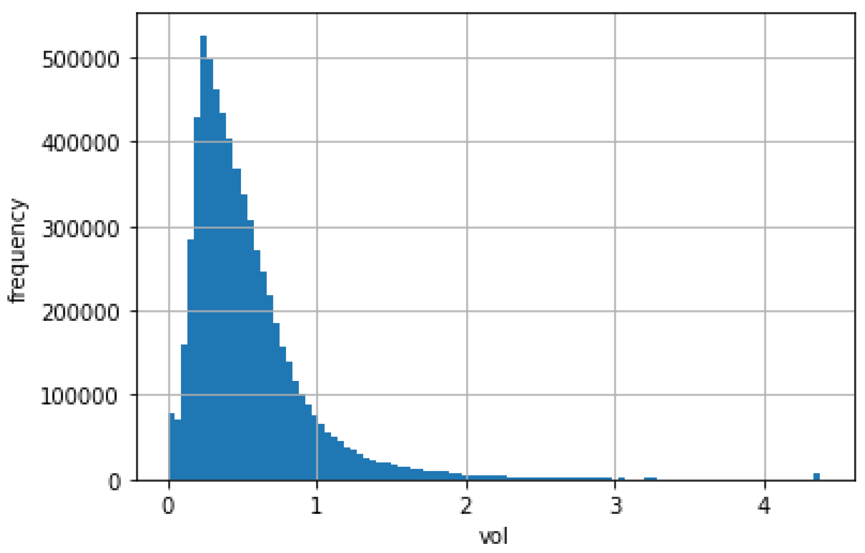
In this work, a set of 3577 American shares for the period from 2008 to 2020, sampled daily, has been used. The volatility of stock i at time t, $v_i\left(t\right)$, is calculated as the standard deviation of the log-returns of one year (250 trading days) ending at t. Other values of the time interval provide qualitatively similar results.

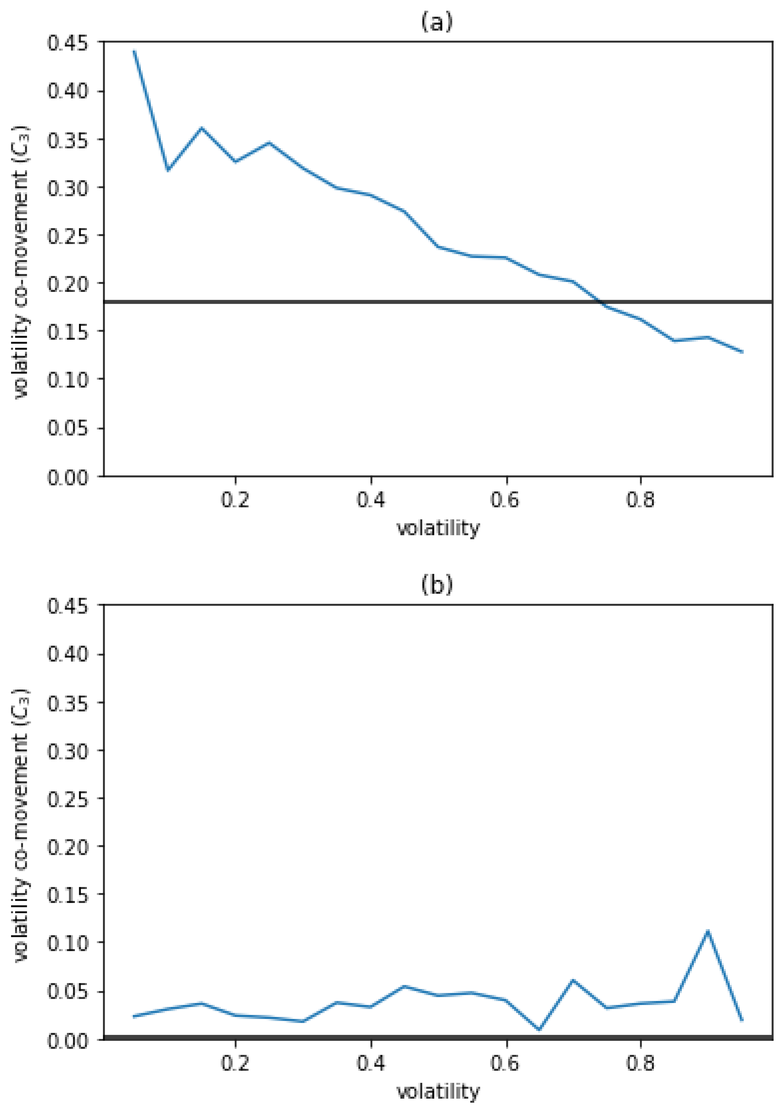
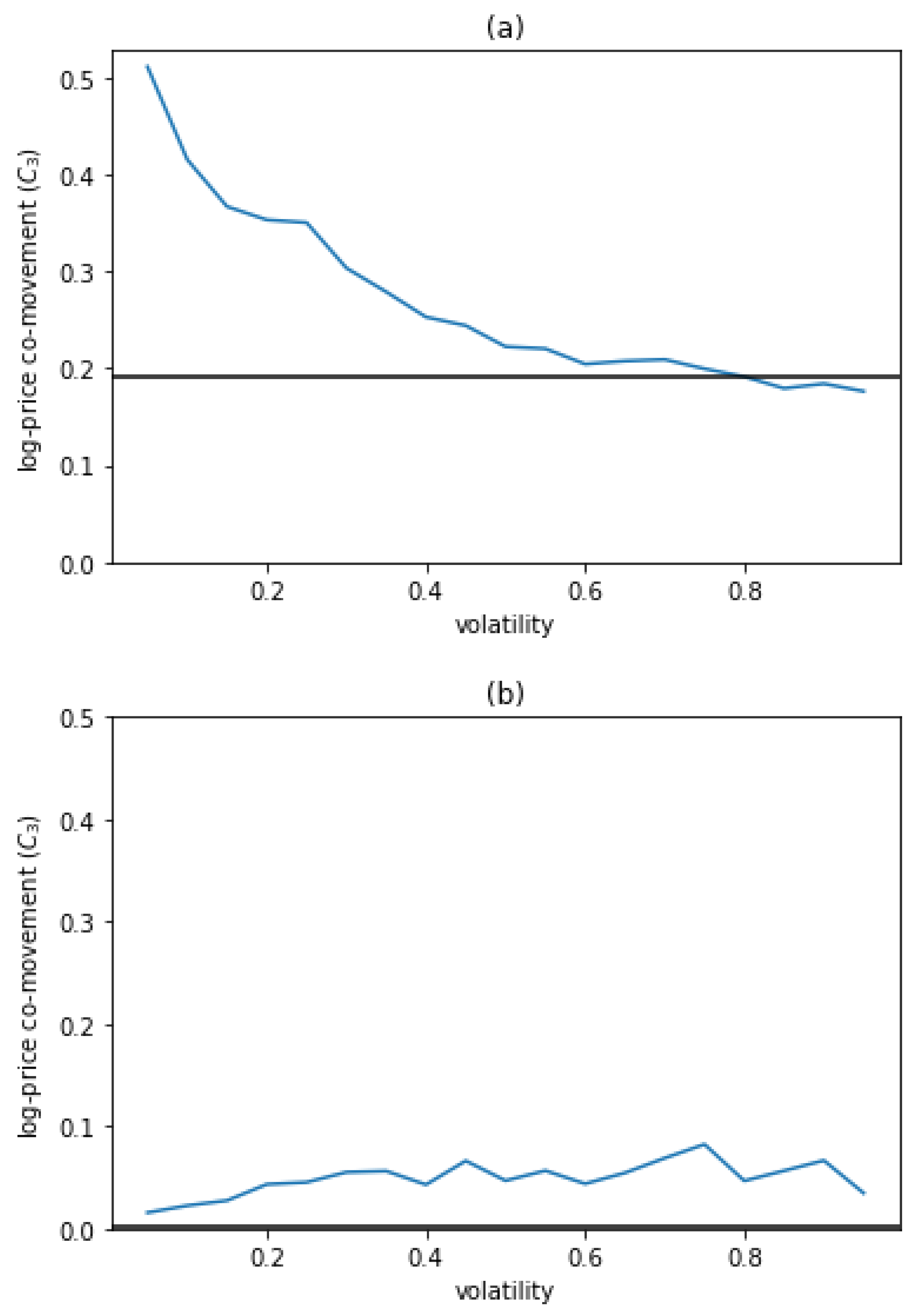
The calculations of $C_{3t}\left(\tau \right)$ and $C_3\left(\tau \right)$ are performed with the bare data $y_i\left(t\right)$ and with $y_i\left(t\right)-m\left(t\right)$. This can serve then to identify the origin of co-movement: if it disappears when the motion of the center of mass is subtracted, there are no important dynamic correlations between individual stocks; on the other hand, if it remains after the center of mass is subtracted, it indicates the existence of dynamic correlations among stocks or groups of stocks.

It must be noted that, different from other techniques in the literature, the present method allows us to analyze the whole set of stocks in a given market, or a particular subset.

3. Results

Previous results have shown that $C_3\left(\tau \right)$ indeed captures the co-movement in the stocks log-price, but also that the overall co-movement can be corrected almost completely subtracting the index [29], defined as the average log-price. Here, we focus on the co-movement in volatility of the sample of stocks using the function $C_3$ defined above. In this case, $y_i$ stands for the volatility. Bare volatility or the deviation from the mean (termed market) is also considered to identify the source of co-movement. Furthermore, in addition to averaging $C_{3t}\left(\tau \right)$ over all pairs of particles, partial averaging over stocks i of similar volatility are also performed. This allows us to conclude correlations, or absence of correlations, between stocks with different volatility.

3.1. Volatility Co-Movement along Time

For the analysis of volatility co-movement over time, we have studied the value $C_{3t}\left(20\right)$ over time t, which is the degree of co-movement after 20 trading days (around one month). Scheme 1 shows the function $C_{3t}\left(20\right)$ vs. t in the period 2008 to 2020 using the bare volatility (upper panel), or subtracting the mean (lower panel). Scheme 1a shows that the volatility co-movement varies strongly over time, with the highest values occurring in periods where some type of crisis has occurred. In the 2008–2009 period, the volatility co-movement reached values above 0.8, which corresponds to the last financial crisis experienced. In mid-2010 and 2011, values close to 0.8 were also observed, corresponding to the flash crash and the Eurozone debt crisis. In 2012–2013, values between 0.6 and 0.8 were also quite high, corresponding to a year of high volatility and recurrent uncertainty due to the new US fiscal policies. Finally, in 2020, values of the volatility of 0.8 were again reached due to the recent crisis from COVID 19. The results obtained are in line with the work of Tseng and Li [35], Trinidad et al. [36] and López García et al. [29], where the co-movement was analyzed with respect to price.

In Scheme 1b, the co-movement is calculated by subtracting the market from the volatility, i.e., using $y_i\left(t\right)=v_i\left(t\right)-m\left(t\right)$ instead of $v_i\left(t\right)$, where the market (equivalent to the center of mass in physical systems) is calculated with an equal weight, $m\left(t\right)=<v_i\left(t\right){>}_i$. In this case, the co-movement is very close to 0, indicating that there is hardly any co-movement in volatility in the sample; thus, we can conclude that the market explains almost completely the volatility co-movement of the stocks. This finding follows a similar result with the log-price co-movement found in [29], though the effect is a bit stronger in log-price co-movement than in volatility co-movement.

3.2. Co-Movement as a Function of Stock Volatility

Figure 1 shows the histogram of the volatility of all stocks for the period 2008–2020. It is noticed that most stocks have volatilities between 0 and 1, but the distribution extends to values above 4. Given this broad range of volatilities, one may ask if the co-movement shows some dependence on the stocks, classified according to their volatility. Even more, since the volatility changes notably over time, this dependence may have changed in some years, especially in crisis periods. In this section, thus, we study the volatility co-movement for our entire sample of American stocks, classifying the stocks according to their volatility, and we repeat the analysis carrying out the study on an annual basis.

Scheme 2 shows the volatility co-movement for stocks of similar volatility averaged over the whole period without subtracting, and subtracting, the market (upper panel and lower panel, respectively). For this purpose, stocks are classified according to the volatility in bins of width $0.10$, and the summation in the calculation in $C_{3t}\left(20\right)$ is restricted to stocks within the same bin.

In Scheme 2a, the volatility co-movement decreases with the volatility, that is, the stocks with smaller volatility reflect a greater co-movement, and as the value in volatility increases the co-movement is lower. In particular, the co-movement of stocks with low volatility is significantly higher than the average value (considering all stocks and the whole period), marked by the horizontal black line at $0.18$. This graph shows that volatility is indeed a relevant factor to consider when studying volatility co-movement.

In Scheme 2b, the average volatility is subtracted for the calculation of the co-movement. The results are very close to zero, and this is reflected in its average (black horizontal line). Nevertheless, for stocks with similar volatility the co-movement is above the average, but still close to zero. Therefore, it can be concluded that the market drives the volatility co-movement of the whole market almost completely, replicating the results of the co-movement in price [29].

The robustness of these results is tested in Scheme 3, where the same analysis is repeated for a much longer time interval for the co-movement; in this case 250 trading days (around one year) are used, in contrast to the 20 days used in Scheme 2. When the market is not subtracted (Scheme 3a), the pattern is similar, or even stronger, to that obtained for 20 trading days (see Scheme 2a). On the other hand, when the market is subtracted, volatility co-movement in 20 trading days (Scheme 2b) is a bit noisier than in the 250 trading days case (Scheme 3b). In the latter, the volatility co-movement cannot be fully explained by the market for stocks with similar high volatility.

We focus now on changes of the distribution of the co-movement as a function of the volatility in time. For this purpose, $C_3\left(\tau \right)$ is calculated as the average of $C_{3t}\left(\tau \right)$ in natural years, and we present the distributions in Scheme 4 for all years, together with the average within this year for all stock pairs (horizontal black lines). As discussed above, periods of crisis can be identified by the high value of the average co-movement (in 2008–2010 it reached 0.4, and in 2020 it was above 0.3), whereas stable years yield a smaller value, close to zero. Even more, the distribution of co-movement also changes notably from crisis to stable periods, being generally higher and flatter in the former, and lower and decreasing in the latter.

In Scheme 5, the volatility co-movement is calculated subtracting the market. As in Scheme 2b, the average of the volatility co-movement remains very close to zero, regardless of the year, even in 2008, 2009, 2010 and 2020. Accordingly, the distribution of co-movement stays close to zero for all volatilities and years. This result confirms that the co-movement among stocks of similar volatility can be interpreted as uncorrelated fluctuations around the mean.

To get further insight into the cooperative dynamics of stocks, and how this changes between crisis and stable periods, we study the co-movement in log-price as a function of stock volatility for the same period. This is performed with the function $C_{3t}\left(\tau \right)$ calculated using the log-price as $y_i\left(\tau \right)$, and restricting the summation to stocks with the volatility within the same bin. The results are shown in Scheme 6: in the upper panel the bare co-movement in the log-price is presented, whereas the lower panel presents the results for the log-price corrected with the mean. A rather high degree of price co-movement in stocks with low volatilities is noticed in Scheme 6a, which decreases as the volatility increases. Again, the co-movement is practically zero when the market is subtracted (Scheme 6b).

It is interesting to note the similarities between this Scheme and Scheme 2, despite the co-movement of different quantities being studied. Even more, the year-by-year study (not shown), that is, the equivalent to Scheme 4 and Scheme 5, with log-price co-movement instead of volatility co-movement is very similar to Scheme 4 and Scheme 5. In addition, if the log-price co-movement in 250 trading days is considered, see Scheme 7, the pattern is again similar to the case of volatility co-movement (Scheme 3) and also similar to log-price co-movement in 20 days (Scheme 6), especially in the case when the market is not subtracted. Note also the very high degree of log-price co-movement for stocks with similar low volatility.

These results, concerning the stability of the distributions, similarity of the results of the price or volatility co-movement, as well as the identification of crisis and stable periods, indicates that the volatility is a key factor for assessing and classifying the dynamics of stocks, and in particular the collective motions. Additionally, the average volatility (or market) drives most of the co-movement in the market.

Co-Movement Maps

To take a step further in the study of co-movement in volatility, maps have been created to show the volatility co-movement among stocks of different volatilities. As discussed previously, stocks are classified according to the volatility in bins of width $0.1$, and the summation over i and j in the definition of $C_{3t}\left(\tau \right)$ is restricted to stocks belonging to the first and second bins, respectively. In these maps the intensity of co-movement is graduated with colors ranging from intense red (high co-movement in the same direction) to intense blue (high co-movement in the opposite direction), leaving white as the color that expresses the non-existence of co-movement.

The first maps are shown in Scheme 8, where we study the co-movement in volatility using the two calculation methods (subtracting and without subtracting the market, for the upper and lower panel, respectively), for the period from 2008 to 2020. Scheme 8a shows in all its boxes the red color, indicating a direct co-movement in volatility between stocks with different degrees of volatility. Stronger co-movement is observed in the diagonal, showing that stocks of similar volatility change more cooperatively than stocks of different volatility, as anticipated in Scheme 2a. Accordingly, the lowest degree of co-movement is observed between stocks of large and small volatility, and vice versa.

On the other hand, Scheme 8b is almost white, so it hardly shows the existence of co-movement in volatility, which supports the results obtained in Scheme 2b when we subtract the market, now for the full sample of stocks. This result confirms that most of the cooperative motion is in fact driven by the market, calculated as the simple average over all stocks, but not all of it. In fact, an increase in the co-movement can be noticed around the diagonal for large values of the volatility.

In Scheme 9, we again perform the study of log-price co-movement as a function of volatility to check whether the same patterns as in the previous section apply. The results again reflect very similar results as in the volatility co-movement, showing in Scheme 9a a predominance of red, indicating a direct log-price co-movement among stocks with different degrees of volatility, with the maximum co-movement among stocks of low volatility. On the other hand, in Scheme 9b, the colors are very soft and almost white, reflecting the scarce existence of log-price co-movement once the market is subtracted. Compared to the volatility co-movement, however, these distributions are flatter, but the lowest values are still obtained for stocks with very different volatility.

In Scheme 10, we present the volatility co-movement maps year by year without subtracting the market. It is clearly noted that the years more affected by crises, which presented a higher average of co-movement in Scheme 4, are the years with the most intense reds; these are 2008, 2009, 2010 and 2020. In most cases, the maximum values of $C_3\left(20\right)$ are obtained among stocks of low and similar volatility, whereas the minima are usually found in stocks of large volatility. Some peculiar cases are 2013, where the co-movement between stocks of very low volatility and any other stock is negative or very small. On the other hand, 2014 and 2017 show an increased co-movement in this case.

In Scheme 11, the volatility co-movement subtracting the market is studied, which again is close to zero (with values between −0.2 and 0.2). In this occasion, blue colors appear in some locations, particularly when stocks of small and large volatility are correlated, indicating an inverse co-movement between the stocks. Even so, crises years are not fully corrected with the market, and the maximum values of $C_3\left(20\right)$ are observed for these years. Additionally, within a year, the largest co-movement is observed for stocks of similar but large volatility.

Comparing Scheme 10 and Scheme 11, co-movement in volatility appears as a powerful and robust tool to identify crisis periods, either with the market accounted for or without it. However, differences are noticed in particular years, where the shape of the distribution changes notably. For instance, year 2013 showed a peculiar behavior using the bare volatility, whereas in Scheme 11 this is fully corrected, and all co-movement has disappeared, indicating that most stocks follow the average with no other correlated motion. More interestingly, year 2020 can be identified as a crisis period, but when subtracting the market, it shows the typical behavior of stable years (such as 2019 or 2017). This points to a different dynamic, and origin, in the crisis in 2020 from the crisis in 2008–2010.

4. Conclusions

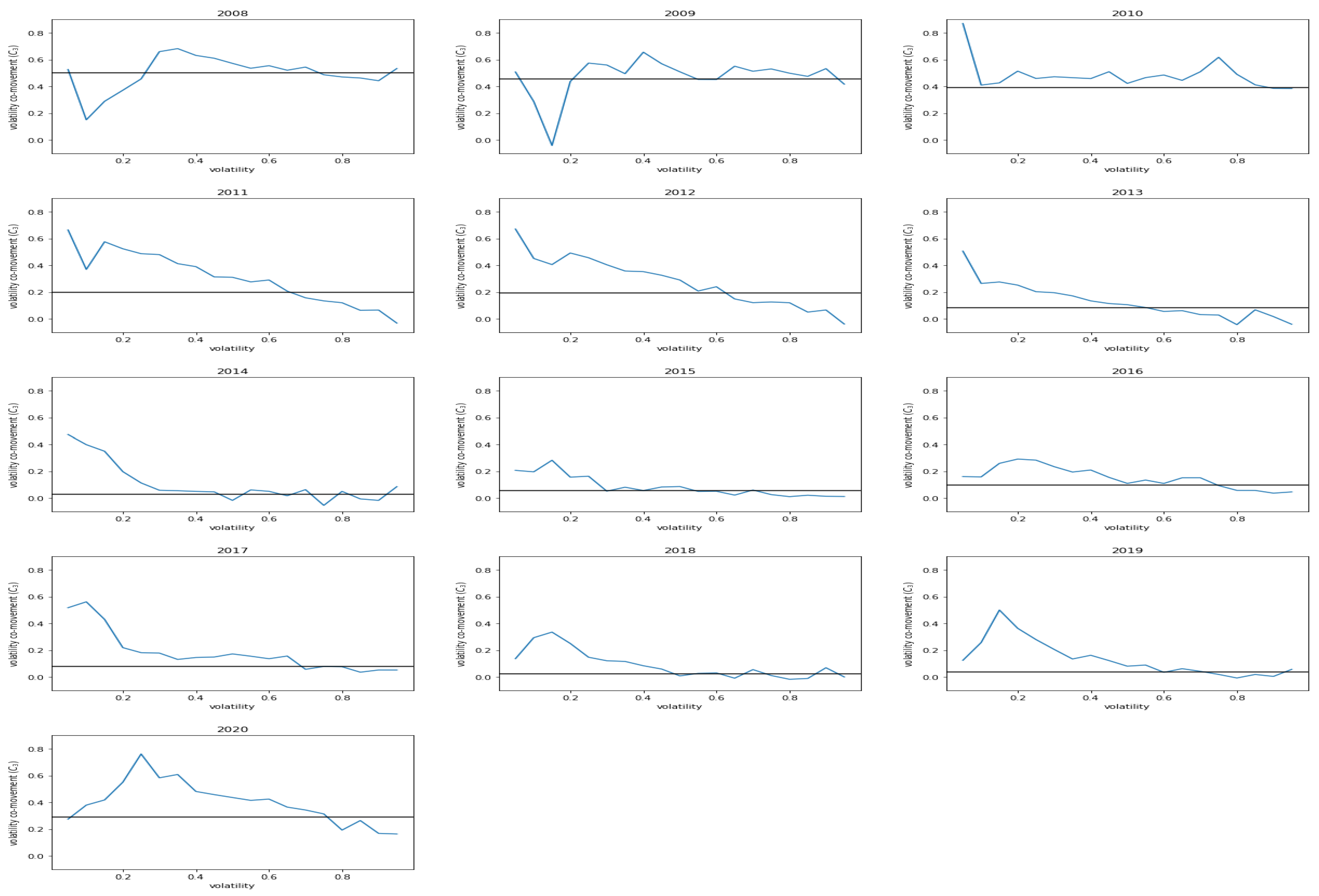
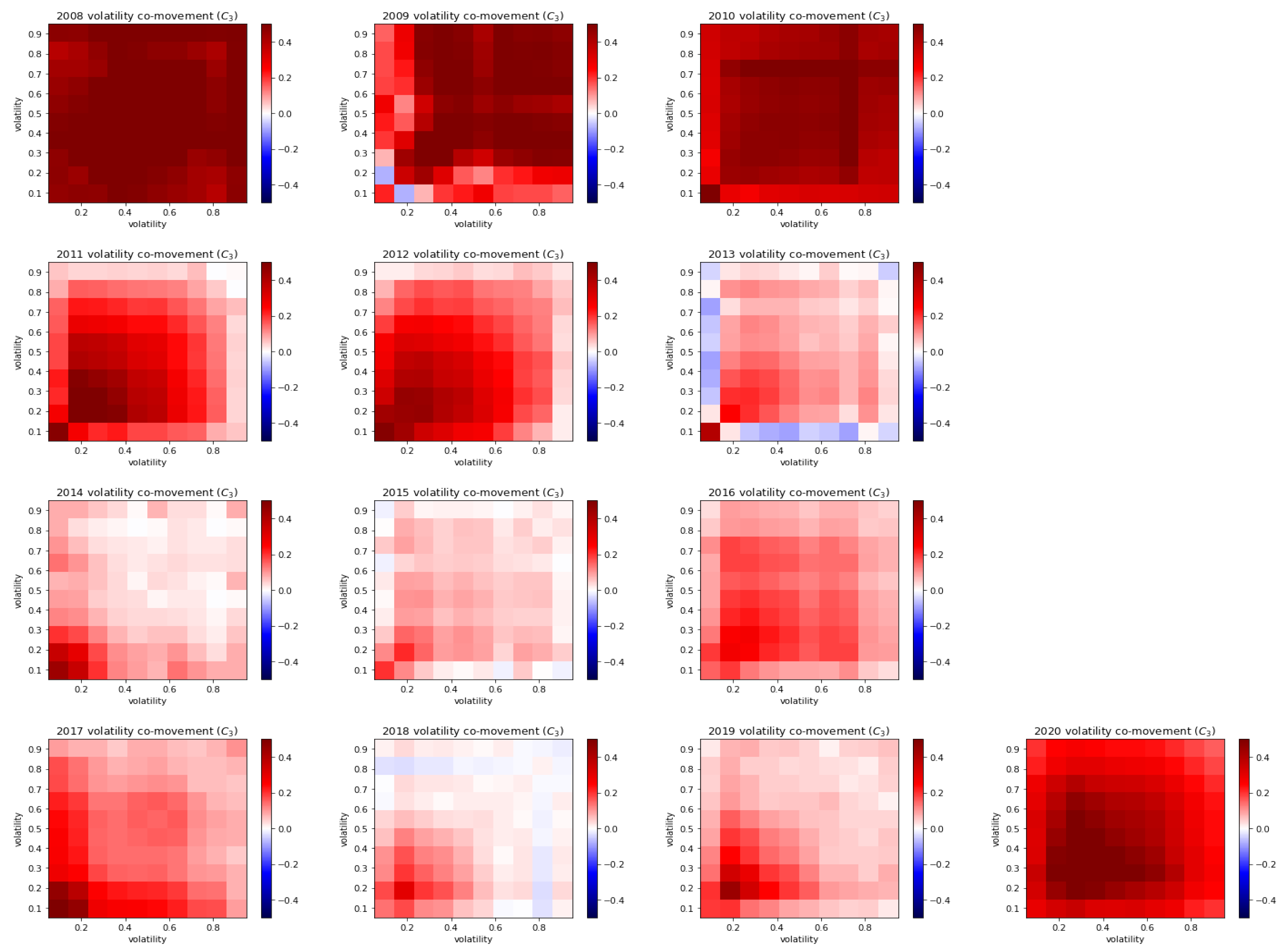
In this paper we use a function borrowed from the analysis of cooperative dynamics in physical systems of colloidal particles to study the co-movement in the volatility of stocks within a single market. A total of 3577 American shares, sampled daily from 2008 to 2020, are analyzed. The period includes the financial crisis in 2008–2010, and COVID19 crisis in 2020. We focus on the co-movement in two main factors: volatility and market. The contribution to the total co-movement from different stocks is classified according to the stock volatility. The methodology allows us to identify the origin of the co-movement and conclude if it is caused by an external agent or correlation among stocks.

Globally, stocks with low volatility have a greater volatility and log-price co-movement than the general market co-movement. In addition, co-movement between stocks of similar volatility is typically larger than co-movement between stocks of different volatility. Negative co-movement is found, in some years, between stocks of very different volatility.

Interpreting this analysis within the background of many-body physics, the market index is defined as the average over all stocks, similar to the center of mass. We study, thus, the volatility (and log-price) co-movement after subtracting the market. The results for the co-movement are very close to zero in both cases, indicating that the market explains the general co-movement to a great extent. These results are similar to those reported by Lopez-Garcia et al. [29] for the log-price co-movement. Our results also show that the market factor is highly significant, as Lopez-Garcia et al. [37] suggested, for asset pricing and portfolio risk and indicates that dynamic correlations between stocks are rare, but relevant only in selected periods, mainly the crisis.

On the other hand, it is observed that both volatility and log-price co-movement of the general market are much higher during crisis periods. Similar results are shown by Trinidad et al. [36] or Tseng et al. [35]. In these periods, stocks with low volatility have a great co-movement, not only with other stocks with low volatility (that they have in general), but also with stocks with greater volatilities, resulting in different distributions of co-movement in crisis and stable periods. Studying the volatility distribution of the co-movement thus serves to identify and characterize crisis periods as well as provide further insight into the dynamics of stock markets.

Finally, the proposed method to study co-movement should be seen as a method to study the co-movement of the full market (or a subgroup of stocks) and can be used to study the influence of a factor or variable (in this paper we have used the volatility) in the log-price or volatility co-movement.

Our findings could also be helpful to approach other problems, such as portfolio diversification. We showed that stocks with low volatilities usually have a high degree of co-movement (both in log-price and volatility); thus, some questions arise with respect to the portfolio: Is a portfolio with stocks of low volatility riskier since they will have a high degree of co-movement? Is it better to construct a portfolio with stocks of different volatilities, as suggested by the fact that they will have a lower degree of co-movement? What about the risk of a portfolio of stocks with high volatility, which tend to have a lower degree of co-movement? These questions represent future promising research lines.

Another implication of our findings is that during crisis periods, the co-movement of the general market increases significantly, and the co-movement between stocks with different volatilities is very high, in comparison with the co-movement between stocks with different volatilities in other periods. Hence, a portfolio that can be considered well diversified in non-crisis periods will probably be much riskier during a crisis, since the diversification fails to work during crisis periods.

To conclude, another future research line is to study with the proposed method the co-movement of other asset pricing factors to see if stocks with a similar factor will have higher or lower co-movement than the general market.

References

1. Meese, R.; Rogoff, K. Empirical exchange rate models of the seventies: Do they fit out of sample? J. Int. Econ. 1983, 14, 3–24. [Google Scholar] [CrossRef]
2. Roll, R. R2. J. Financ. 1988, 43, 541–566. [Google Scholar] [CrossRef]
3. Katsiampa, P. Volatility co-movement between Bitcoin and Ether. Financ. Res. Lett. 2019, 30, 221–227. [Google Scholar] [CrossRef] [Green Version]
4. Domowitz, I.; Hansch, O.; Wang, X. Liquidity commonality and return co-movement. J. Financ. Mark. 2005, 8, 351–376. [Google Scholar] [CrossRef]
5. Byrne, J.P.; Cao, S.; Korobilis, D. Decomposing global yield curve co-movement. J. Bank. Financ. 2019, 106, 500–513. [Google Scholar] [CrossRef]
6. Parsley, D.; Popper, H. Return comovement. J. Bank. Financ. 2020, 112, 105–223. [Google Scholar] [CrossRef]
7. Edwards, S.; Susmel, R. Interest-rate volatility in emerging markets. Rev. Econ. Stat. 2003, 85, 328–348. [Google Scholar] [CrossRef]
8. Lee, S.J. Volatility spillover effects amongsix Asian countries. Appl. Econ. Lett. 2009, 16, 501–508. [Google Scholar] [CrossRef]
9. Hamao, Y.; Masulis, R.W.; Ng, V. Correlation in price changes and volatility across international stock markets. Rev. Financ. Stud. 1990, 3, 281–307. [Google Scholar] [CrossRef]
10. Susmel, R.; Robert, F. Engle Hourly volatility spillovers between international equity markets. J. Int. Money Financ. 1994, 13, 3–25. [Google Scholar] [CrossRef]
11. Fleming, J.; Kirby, C.; Ostdiek, B. Information and volatility linkages in the stock, bond, and money markets. J. Financ. Econ. 1998, 49, 111–137. [Google Scholar] [CrossRef]
12. Dávila, E.; Parlatore, C. Trading Costs and Informational Efficiency. NBER Working Paper. 2019. Available online: https://www.nber.org/papers/w25662 (accessed on 13 February 2021).
13. Jondeaua, E.; Rockinger, M. Conditional volatility, skewness, and kurtosis: Existence, persistence, and comovements. J. Econ. Dyn. Control 2003, 27, 1699–1737. [Google Scholar] [CrossRef] [Green Version]
14. Gabudean, R. Volatility Co-Movement. SSRN 2005. [Google Scholar] [CrossRef]
15. Calvet, L.E.; Fisherd, A.J.; Samuel, B. Thompsona. Volatility comovement: A multifrequency approach. J. Econom. 2006, 131, 179–215. [Google Scholar] [CrossRef] [Green Version]
16. Modi, A.G.; Patel, B.; Patel, N.R. The Study on co-Movement of Selected Stock Markets. Int. Res. J. Financ. Econ. 2010, 47, 170–185, SSRN. Available online: https://ssrn.com/abstract=2660643 (accessed on 2 March 2021).
17. Chen, J.; Kobayashi, M.; McAleer, M. Testing for volatility co-movement in bivariate stochastic volatility models. J. Jpn. Stat. Soc. 2017, 47, 13–36. [Google Scholar] [CrossRef] [Green Version]
18. Zhang, Y.; Ding, S. Return and volatility comovement in commodity futures markets: The effects of liquidity risk. Quant. Financ. 2018. [Google Scholar] [CrossRef]
19. Bašta, M.; Molnár, P. Oil market volatility and stock market volatility. Financ. Res. Lett. 2018, 26, 204–214. [Google Scholar] [CrossRef]
20. Huang, W.; Wang, D. Systemic importance analysis of chinese financial institutions based on volatility spillover network. Chaos Solitons Fractals 2018, 114, 19–30. [Google Scholar] [CrossRef]
21. Fernández-Avilés, G.; Montero, J.M.; Sanchis-Marco, L. Extreme downside risk co-movement in commodity markets during distress periods: A multidimensional scaling approach. Eur. J. Financ. 2020, 12, 1207–1237. [Google Scholar] [CrossRef]
22. Zheng, Y.; Wang, Z.; Huang, Z.; Jiang, T. Comovement between the Chinese Business Cycle and Financial Volatility: Based on a DCCMIDAS Model. Emerg. Mark. Financ. Trade. Emerg. Mark. Financ. Trade 2019, 56, 1–15. [Google Scholar] [CrossRef]
23. Wang, S.; Guo, Z. A study on the co-movement and influencing factors of stock markets between China and the other G20 members. Int. J. Financ. Econ. 2019, 25, 1–20. [Google Scholar] [CrossRef] [Green Version]
24. Liu, X.; Jiang, C. The dynamic volatility transmission in the multiscale spillover network of the international stock market. Phys. A 2020, 560, 125144. [Google Scholar] [CrossRef]
25. Qiao, X.; Zhu, H.; Hau, L. Time-frequency co-movement of cryptocurrency return and volatility: Evidence from wavelet coherence analys. Int. Rev. Financ. Anal. 2020, 71, 101541. [Google Scholar] [CrossRef]
26. Clara-Rahola, J.; Puertas, A.M.; Sánchez-Granero, M.A.; Trinidad-Segovia, J.E.; de las Nieves, F.J. Diffusive and arrestedlike dynamics in currency exchange markets. Phys. Rev. Lett. 2017, 118, 068301. [Google Scholar] [CrossRef] [PubMed] [Green Version]
27. Sánchez-Granero, M.A.; Trinidad-Segovia, J.E.; Clara-Rahola, J.; Puertas, A.M.; de las Nieves, F.J. A model for foreign exchange markets based on glassy Brownian systems. PLoS ONE 2017, 12, e0188814. [Google Scholar] [CrossRef] [Green Version]
28. Puertas, A.M.; Sánchez-Granero, M.A.; Clara-Rahola, J.; Trinidad-Segovia, J.E.; de las Nieves, F.J. Stock markets: A view from soft matter. Phys. Rev. E 2020, 101, 032307. [Google Scholar] [CrossRef]
29. López-García, M.N.; Sánchez-Granero, M.A.; Trinidad-Segovia, J.E.; Puertas, A.M.; de las Nieves, F.J. A new look on financial markets co-movement through cooperative dynamics in many-body physics. Entropy 2020, 22, 954. [Google Scholar] [CrossRef] [PubMed]
30. Yura, Y.; Takayasu, H.; Sornette, D.; Takayasu, M. Financial brownian particle in the Layered order-Book fluid and fluctuation-dissipation relations. Phys. Rev. Lett. 2014, 112, 098703. [Google Scholar] [CrossRef] [PubMed] [Green Version]
31. Fernández-Nieves, A.; Puertas, A.M. (Eds.) Fluids, Colloids and Soft Materials; Wiley: Hoboken, NJ, USA, 2016. [Google Scholar]
32. Langer, J. The mysterious glass transition. Phys. Today 2007, 60, 8. [Google Scholar] [CrossRef] [Green Version]
33. Muranaka, T.; Hiwatari, Y. β relaxation in a highly supercooled state via molecular dynamics simulation. Phys. Rev. E 1995, 51, R2735(R). [Google Scholar] [CrossRef] [PubMed]
34. Zahn, K.; Lenke, R.; Maret, G. Two-stage melting of paramagnetic colloidal crystals in two dimensions. Phys. Rev. Lett. 1999, 82, 2721. [Google Scholar] [CrossRef] [Green Version]
35. Tseng, J.J.; Li, S.P. Asset returns and volatility clustering in financial time series. Phys. A Stat. Mech. Appl. 2011, 390, 1300–1314. [Google Scholar] [CrossRef] [Green Version]
36. Trinidad Segovia, J.E.; Fernández-Martínez, M.; Sánchez-Granero, M.A. A novel approach to detect volatility clusters in financial time series. Phys. A Stat. Mech. Appl. 2019, 535, 122452. [Google Scholar] [CrossRef]
37. López-García, M.N.; Trinidad-Segovia, J.E.; Sánchez-Granero, M.A.; Pouchkarev, I. Extending the Fama and French model with a long term memory factor. Eur. J. Oper. Res. 2021, 291, 421–426. [Google Scholar] [CrossRef]
Scheme 1. Volatility monthly co-movement ( C 3 t ( 20 ) ) of the whole market from 2008 to 2020. Blue line is the daily co-movement, while the black line is a moving average of the blue line with a time window of 60 trading days; (a) the market is not subtracted; (b) the market is subtracted.
Mathematics 09 00598 sch001
Figure 1. Histogram of the volatility of all stocks in the period 2008–2020.
Mathematics 09 00598 g001
Scheme 2. Volatility monthly co-movement ( C 3 ( 20 ) ) for stocks of similar volatility for the period 2008–2020; (a) the market is not subtracted; (b) the market is subtracted.
Mathematics 09 00598 sch002
Scheme 3. Volatility monthly co-movement ( C 3 ( 250 ) ) for stocks of similar volatility for the period 2008–2020; (a) the market is not subtracted; (b) the market is subtracted.
Mathematics 09 00598 sch003
Scheme 4. Volatility monthly co-movement for each year in the period 2008–2020.
Mathematics 09 00598 sch004
Scheme 5. Volatility monthly co-movement (subtracting the market) for each year in the period 2008–2020.
Mathematics 09 00598 sch005
Scheme 6. Log-price monthly co-movement ( C 3 ( 20 ) ) as a function of volatility during the period 2008–2020; (a) the market is not subtracted; (b) the market is subtracted.
Mathematics 09 00598 sch006
Scheme 7. Log-price yearly co-movement ( C 3 ( 250 ) ) as a function of volatility during the period 2008–2020; (a) the market is not subtracted; (b) the market is subtracted.
Mathematics 09 00598 sch007
Scheme 8. Volatility monthly co-movement among stocks of different (and similar) volatilities. (a) Without subtracting the market; (b) subtracting the market.
Mathematics 09 00598 sch008
Scheme 9. Log-price monthly co-movement among stocks of different (and similar) volatilities. (a) Without subtracting the market; (b) subtracting the market.
Mathematics 09 00598 sch009
Scheme 10. Volatility monthly co-movement among stocks of different (and similar) volatilities for each year from 2008 to 2020 (without subtracting the market).
Mathematics 09 00598 sch010
Scheme 11. Volatility monthly co-movement among stocks of different (and similar) volatilities for each year from 2008 to 2020 (subtracting the market).
Mathematics 09 00598 sch011
Publisher’s Note: MDPI stays neutral with regard to jurisdictional claims in published maps and institutional affiliations.