Article

Cox Processes Associated with Spatial Copula Observed through Stratified Sampling

1
Department of Mathematics and Computer Sciences, Université des Antilles, 97157 Pointe-à-Pitre, France
2
Université d’Etat d’Haiti, HT6110 Port-au-Prince, Haiti
*
Author to whom correspondence should be addressed.
Mathematics 2021, 9(5), 524; https://doi.org/10.3390/math9050524
Submission received: 31 January 2021 / Revised: 24 February 2021 / Accepted: 25 February 2021 / Published: 3 March 2021

Abstract

:
Cox processes, also called doubly stochastic Poisson processes, are used for describing phenomena for which overdispersion exists, as well as Poisson properties conditional on environmental effects. In this paper, we consider situations where spatial count data are not available for the whole study area but only for sampling units within identified strata. Moreover, we introduce a model of spatial dependency for environmental effects based on a Gaussian copula and gamma-distributed margins. The strength of dependency between spatial effects is related with the distance between stratum centers. Sampling properties are presented taking into account the spatial random field of covariates. Likelihood and Bayesian inference approaches are proposed to estimate the effect parameters and the covariate link function parameters. These techniques are illustrated using Black Leaf Streak Disease (BLSD) data collected in Martinique island.

1. Introduction

Statistical Inference with spatial data requires to take into consideration a strong possibility of spatial dependency. In case of observations corresponding to the realization of a point process, the available data can be either point spatial locations or counts of points in spatial units [1,2]. These authors developed the mathematical theory of point processes which are used in many areas for describing event occurrences, like earthquakes, accidents, pest infestations, disease appearances, neuronal spikes, and many other situations [3,4,5,6,7]. Thus, a wide range of scientific applications can be cited, for example: ecology, epidemiology, geology, forestry, neurophysiology. De Oliveira [8] described a class of models for geostatistical count data generalizing the class proposed by Diggle et al., in 1998 [9]. Diggle [10] discussed about different spatial and spatio-temporal point process models, along with marked and multivariate counting processes. Wakefield [11] presented a critical review of spatial count data analysis methods for either disease mapping or spatial regression. He emphasizes the importance of the nature of variability in spatial risk and the fact that models must account for both spatial and non-spatial variability. Ickstadt and Wolpert [12] introduced a class of Bayesian hierarchical spatial models taking into account dependence on unobserved or unreported covariates. Examples and illustrations of state-of-the art developments in statistics for spatial data are presented in Cressie [13] with focus on lattice data, geostatistical data and point patterns. Sain and Cressie [14] emphasize that incorporating general forms of correlation is important in building spatial models for lattice data. Our goal is to consider Gamma-distributed effects which are spatially correlated. Given this constraint of marginal Gamma distributions, joint laws allowing such marginal properties, along with spatial dependence, are rare. This is the reason why we use the copula theory which allows both marginal laws and spatial dependence or spatial effects [15]. A spatial copula as defined in Durocher et al. [16] provide a full probabilistic model. Conversely, a covariance function describes only the covariance between marginal distributions except in the case of a multivariate Gaussian distribution which is fully specified by its expectation and covariance matrix.
In this paper, we consider count observations from a doubly stochastic Poisson process also called Cox process [8,17,18,19,20] on a measured space ( X , B , ν ) and driven by a random measure Λ such that there exists a positive random field λ ( . ) verifying:
B B , Λ ( B ) = B λ ( x ) ν ( d x ) .
λ ( . ) is the process intensity with respect to the reference measure ν . Its state space is X and Λ ( . ) denotes its intensity measure. For example, ν can be the Lebesgue measure or a counting measure for individuals at risks.
The idea behind the model based on a Cox process is that environmental heterogeneity can generate overdispersion but also dependency. The counting measure N associated with such a Cox process verifies:
B B , N ( B ) P ( Λ ( B ) ) | Λ ,
which means that, conditionally to Λ , the count N ( B ) follows the Poisson distribution with parameter Λ ( B ) .
A well known result on doubly stochastic Poisson process is that stochasticity on Λ generates overdispersion: for any element B of B such that E ( Λ ( B ) ) > 0 and V a r ( Λ ( B ) ) > 0 , the dispersion index is
V a r ( N ( B ) ) E ( N ( B ) ) = E ( Λ ( B ) ) + V a r ( Λ ( B ) ) E ( Λ ( B ) ) = 1 + V a r ( Λ ( B ) ) E ( Λ ( B ) ) > 1 .
If Λ ( B ) is not a proper random variable or in other terms if V a r ( Λ ( B ) ) = 0 , then the dispersion index is equal to unity, what corresponds to a standard Poisson process. It is worth pointing out that modeling a Cox process is equivalent to modeling either its intensity λ ( . ) or its driving measure Λ ( . ) . For example, Wolpert and Ickstadt [21] constructed λ as a linear combination of location-specific attributes and a kernel mixture measure associated with an independent-increment infinitely divisible random measure.
The general model studied in this paper is as follows. We assume that X has a finite n-partition X j j J and:
λ ( x ) = j J A j f θ Z ( x ) 𝟙 X j ( x ) ,
where A j is a positive random variable, and 𝟙 X j stands for the indicator function of X j . We denote by Z ( x ) the random vector of q covariates at point x and by f θ the positive link function defined on Z ( X ) and parameterized by θ . Therefore, Z is a random field taking values in a q-dimensional space and can not be observed entirely in practice. However we assume that for a given sampling unit, we have relevant summaries providing information on the Cox process. The unknown parameter θ belongs to R q with q q and has to be estimated from observations of the Cox process and its q covariate summaries. Our aim is to present tools for statistical inference with data from the counting measure associated with a Cox process which intensity function given by Equation (3), along with partial observations of its spatial covariates. This inference is on θ and also about the P A j parameters.
It should be noted that we consider count data derived from a stratified sampling procedure [22], whereas, in the literature, for each stratum X j , complete observations are available for the count measure and for the covariates [11], particularly for disease mapping [23]. We are, therefore, interested in a situation encountered in practice where the observations in each stratum are partial and carried out across sampling units. Furthermore, the spatial effects ( A j ) j J are not necessarily mutually independent. Such a spatial correlation can be modeled by means of copula functions: Xue-Kun Song [24] presented a class of multivariate dispersion models based on multivariate Gaussian copula, Masarotto [25] identified Gaussian copula models for marginal regression analysis, Krupskii and Genton [26] proposed copula models for spatial data repeatedly observed in time, and Lee [27] developed a copula-based model for multisite precipitation occurrences.
In Section 2, distributional properties of the counting measure N are presented. A set of sampling units is considered in Section 3 with general features met in practice: the units are disjoint and entirely included in one of the partition elements X j . Firstly, the expressions of the likelihood conditional on the covariate field Z and the effect A j are provided. Following Wakefield [11], spatially correlated log-normal effects are considered. This leads to observed counts in sampling units following the multivariate Poisson-log normal distribution [28]. Secondly, we show that the joint distribution of counts in the sampling units for each X j is negative multinomial when the effects are gamma-distributed, and also that correlated gamma-distributed effects lead to dependent negative multinomial counts. Spatial correlations between effects are taken into account by means of Gaussian copula associated with Gamma distributed margins. In Section 4, the focus is on estimating the model parameters. In some situations, closed-form estimators may be obtained, but it is generally not the case. Likelihood inference can be performed when the effects are independent. Otherwise, a Markov chain Monte Carlo (MCMC) procedure is proposed in order to perform Bayesian inference [29]. An illustration is provided in 
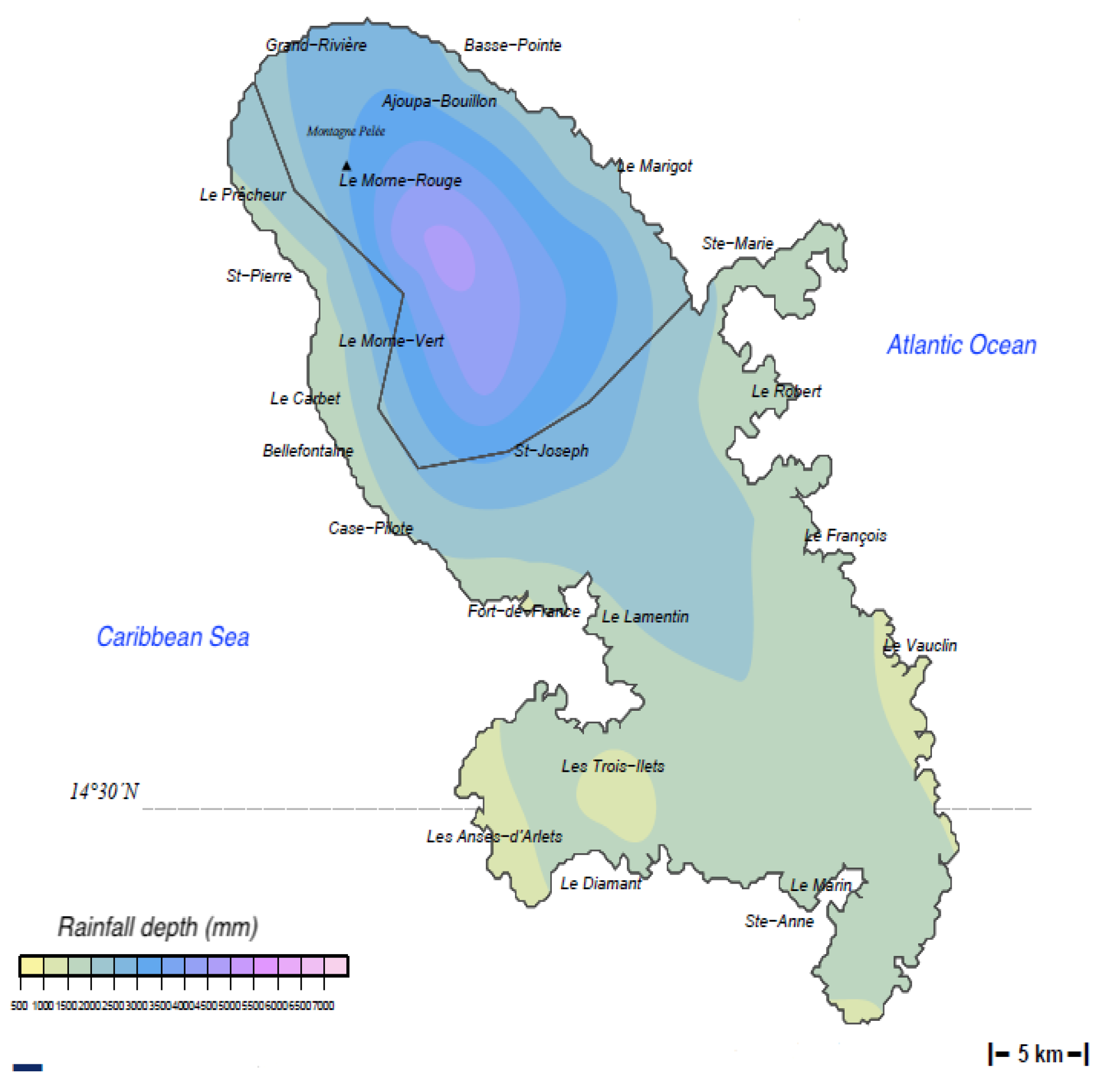
Section 5 from BLSD data collected in Martinique Island within a network coordinated by the DAAL (Direction de l’Alimentation, de l’Agriculture et de la Forêt) and the FREDON Martinique (Fédération REgionale de Défense contre les Organismes Nuisibles de la Martinique).

2. Distributional Properties

In this section, we present the distributional properties associated with the counting measure N. These properties conditional on covariate vector Z give an idea of the dependency between the different spatial zones considered.
For any B in B , let us write
S ν ( B , θ , Z ) = B f θ Z ( x ) ν ( d x ) .
Here, the random measure S ν ( B , θ , Z ) depends on Z only through its restricted random field Z B = ( Z ( x ) ) x B on B.
The following proposition gives the expected number of points conditional on Z and ( A j ) j J :
Proposition 1.
Let N be the counting measure associated with the point process in which intensity is given by Equation (3); then,
B B , E ( N ( B ) | ( A j ) j J , Z ) = j J A j S ν ( B X j , θ , Z ) .
Proof of Proposition 1.
For any element B of B , we have
E ( N ( B ) | ( A j ) j J , Z ) = Λ ( B ) = B λ ( x ) ν ( d x ) = B j J A j f θ Z ( x ) 𝟙 X j ( x ) ν ( d x ) = j J A j B X j f θ Z ( x ) ν ( d x ) = j J A j S ν ( B X j , θ , Z ) ,
which shows (5). □
We have the following results about count correlation:
Proposition 2.
Consider the counting measure N associated with the point process defined by Equation (3). For any ( B 1 , B 2 ) in B 2 , the following equality holds:
C o v ( N ( B 1 ) , N ( B 2 ) | Z ) = ( j , j ) J 2 C o v ( A j , A j | Z ) S ν ( B 1 X j , θ , Z ) S ν ( B 2 X j , θ , Z ) .
Proof of Proposition 2.
From the covariance decomposition formula, we get
C o v ( N ( B 1 ) , N ( B 2 ) | Z ) = C o v E ( N ( B 1 ) | ( A j ) j J , Z ) , E ( N ( B 2 ) | ( A j ) j J , Z ) + E C o v ( N ( B 1 ) , N ( B 2 ) | ( A j ) j J , Z ) .
Since N is a Cox process, the second term of the right-hand side of the above equation is equal to zero so that Equation (5) leads to
C o v ( N ( B 1 ) , N ( B 2 ) | Z ) = C o v ( j J A j B 1 X j f θ ( Z ( x ) ν ( d x ) , j J A j B 2 X j f θ Z ( x ) ν ( d x ) ,
and also to the final result. □
Corollary 1.
Consider the counting measure N associated with the point process defined by Equation (3) and assume the A j are independent conditionally to Z. For any couple ( B 1 , B 2 ) in B 2 ,
C o v ( N ( B 1 ) , N ( B 2 ) | Z ) = j J V a r ( A j | Z ) S ν ( B 1 X j , θ , Z ) S ν ( B 2 X j , θ , Z ) .
Proof of Corollary 1.
From Proposition 2 and conditional independence, whenever any distinct j , j in J, we get C o v ( A j , A j | Z ) = 0 , and the final result follows. □
Corollary 2.
Consider the counting measure N associated with the point process defined by Equation (3) and assume the spatial effect variables ( A j ) j J are mutually independent. Let B 1 and B 2 be two elements of B . If ( j , j ) J 2 , with j j , and B 1 X j , B 2 X j , then
C o v ( N ( B 1 ) , N ( B 2 ) | Z ) = 0 .
Proof of Corollary 2.
From corollary 1, the result is straightforward. □
Corollary 3.
Let B 1 and B 2 be two elements of B . If there exists j in J, such that B 1 , B 2 X j , then
C o v ( N ( B 1 ) , N ( B 2 ) | Z ) = V a r ( A j | Z ) S ν ( B 1 X j ) S ν ( B 2 X j ) .
Proof of Corollary 3.
Both B 1 and B 2 are subsets of X j . Therefore, Proposition 2 give us the final result. □
It is worth noticing that, in the case where A j is a non-degenerate random variable conditional on Z, then V a r ( A j | Z ) > 0 , which implies that C o v ( N ( B 1 ) , N ( B 2 ) | Z ) > 0 .

3. Sampling Theory Results

In this section, we consider a set S of sampling units such that:
(C1) S = { B i j B , i [ [ 1 , n j ] ] , j J } ,
(C2) j J , B i j X j ,
(C3) ( i , i ) [ [ 1 , n j ] ] 2 , i i B i j B i j = .
Condition (C3) means that there is no overlapping sampling units. When these three conditions are verified, we have the following results about the likelihood from the model defined by Equation (3).
Proposition 3.
Let S be a sample verifying conditions (C1), (C2), and (C3). For the model defined by Equation (3), if the joint distribution of ( A j ) j J admits a probability density function g parameterized by β, then the conditional likelihood on A j = a j for S with respect to the counting measure N and ( θ , β ) denoted by L ( θ , β ) ; ( N ( B ) ) B S , ( a j ) j J is equal to
j J i = 1 n j ( a j S ν ( B i j , θ , Z ) ) N ( B i j ) N ( B i j ) ! exp ( a j S ν ( B i j , θ , Z ) ) g ( a j ) j J .
It is worth noticing that this likelihood is conditional on Z.
Proof of Proposition 3.
Since condition (C2) is verified, then B i j X j . Therefore, conditionally to A j and Z, the count N ( B i j ) is distributed according to the Poisson law P ( A j S ν ( B i j , θ , Z ) ) . Furthermore, the N ( B i j ) are independent conditionally to the A j . □
The likelihood given in Proposition 3 is useful for Bayesian approach when prior information on ( A j ) j J are available, as well as sampling algorithms for augmented data. In practice, the A j are not observed. Consequently, the likelihood techniques are based on count observations only. The following corollary provides such a likelihood:
Corollary 4.
Let S be a sample verifying conditions (C1), (C2), and (C3), if the joint distribution of ( A j , j J ) admits a probability density function g parameterized by β, then the unconditional likelihood for S with respect to the counting measure N and ( θ , β ) denoted by L ( θ , β ) ; ( N ( B ) ) B S is equal to
R + n j J i = 1 n j ( a j S ν ( B i j , θ , Z ) ) N ( B i j ) N ( B i j ) ! exp ( a j S ν ( B i j , θ , Z ) ) g ( a j ) j J d a 1 d a n .
Proof of Corollary 4.
The result is straightforward from Proposition 3. □
Many distributions can be used for the joint probability law of ( A j , j J ) which has to be considered as a mixing distribution in the framework of Poisson mixtures [30]. In the case where this joint probability law is a multivariate log-normal distribution LN ( μ , Σ ) with μ R n and Σ a square matrix or order n, then the probability density function g is such that:
g ( a j ) j J = exp 1 2 ( ln ( a ) μ ) t Σ 1 ( ln ( a ) μ ) ( 2 π ) n / 2 ( d e t Σ ) 1 / 2 j J a j ,
where ln ( a ) = ( ln ( a j ) ) j J and n is the cardinality of J.
Following Wakefield [11], for any j in J, we can write A j = exp ( U j + V j ) , where the V j are independent identically distributed according to N ( 0 , σ v 2 ) corresponding to non spatial contribution to overdispersion. On the other hand, the U j are spatial contributions associated with a distance d on X such that ( U j ) j J follows a multivariate normal distribution with C o v ( U j , U k ) = σ u 2 ρ d ( C j , C k ) , where C j and C k are the centroids of X j and X k , respectively. Consequently, C o r ( U j , U k ) = ρ d ( C j , C k ) so that parameter ρ stands for the correlation between U j and U k if d ( C j , C k ) = 1 . We assume that ρ [ 0 , 1 ] . Therefore, in Equation (8), μ is the null vector of R n , and matrix Σ has each diagonal element equal to σ u 2 + σ v 2 , whereas element on line j and column k equal to σ u 2 ρ d ( C j , C k ) . In the case where the mixture distribution is a multivariate log-normal distribution, Equations (7) and (8) provide tools for statistical analysis of counts in sampling units similarly to Aitchison and Ho [28].
An other choice of law for the effect A j is the Gamma distribution with two parameters m j and γ j , where m j is its expectation, and γ j the shape parameter. Equation (9) gives its density function. It is worth noticing that several parameterizations can be met in the literature. We have the following theorem:
Theorem 1.
Let the random measure S ν ( B i j , θ , Z ) be as in Equation (4). For any element j of J, and ( B i j ) i [ [ 1 , n j ] ] elements of B verifying conditions (C2) and (C3), if we assume that A j follows a Gamma distribution Γ ( m j , γ j ) with density function f A j given by:
f A j ( x ) = x γ j 1 Γ ( γ j ) γ j m j γ j exp x γ j m j ,
then:
(i) 
N ( B i j ) i [ [ 1 , n j ] ] follows a multinomial negative distribution,
(ii) 
i [ [ 1 , n j ] ] ,
E ( N ( B i j ) | Z ) = m j S ν ( B i j , θ , Z )
and
V a r ( N ( B i j ) | Z ) = E ( N ( B i j ) | Z ) 1 + E ( N ( B i j ) | Z ) γ j .
(iii) 
For two distinct elements i and i of [ [ 1 , n j ] ] , the following equality holds:
C o v ( N ( B i j , N ( B i j ) | Z ) = m j 2 γ j S ν ( B i j , θ , Z ) S ν ( B i j , θ , Z ) .
Proof of Theorem 1.
( i ) Using the probability generating function of N ( B i j ) i [ [ 1 , n j ] ] , along with the moment generating function of A j , leads us to the result.
In fact, for any j in J, if we write N j = N ( B i j ) i [ [ 1 , n j ] ] , then the probability generating function of N j conditionally to A j and Z at any point ( s 1 , , s n j ) of [ 0 , 1 ] n j is:
G N j | A j , Z ( s 1 , , s n j ) = E i = 1 n j s i N i j | A j , Z = exp A j i = 1 n j ( 1 s i ) S ν ( B i j , θ , Z ) .
Therefore, the probability generating function of N j conditional on Z is such that:
G N j | Z ( s 1 , , s n j ) = E G N j | A j , Z ( s 1 , , s n j )   = E exp A j i = 1 n j ( 1 s i ) S ν ( B i j , θ , Z )   = M A j i = 1 n j ( 1 s i ) S ν ( B i j , θ , Z ) ,
where M A j stands for the moment generating function of A j .
Since A j Γ ( m j , γ j ) , then
G N j | Z ( s 1 , , s n j ) = 1 + m j γ j i = 1 n j ( 1 s i ) S ν ( B i j , θ , Z ) γ j ,
so that N j conditional on Z follows a multinomial negative distribution with parameters m j S ν ( B i j , θ , Z ) i 1 , n j , γ j .
( i i ) and ( i i i ) The first derivative of G N j | Z with respect to s i at point 1 gives us E ( N ( B i j ) | Z ) . The second derivatives of G N j | Z provide in a similar manner the second moments associated with N j . □
Proposition 4.
Let S be a sample verifying conditions (C1), (C2), and (C3). Assume the random variables A j , j J , are mutually independent and distributed according to Γ ( m j , γ j ) as defined by Equation (9). Writing β = ( m j , γ j ) j J , then the likelihood L ( θ , β ) ; ( N ( B ) ) B S for S with respect to the counting measure N and ( θ , β ) is equal to
j = 1 n Γ ( Y + j + γ j ) Γ ( γ j ) γ j m j S ν + ( B j , θ , Z ) + γ j γ j m j m j S ν + ( B j , θ , Z ) + γ j Y + j i = 1 n j S ν ( B i j , θ , Z ) Y i j Y i j ! ,
with Y i j = N ( B i j ) , Y + j = i = 1 n j Y i j and S ν + ( B j , θ , Z ) = i = 1 n j S ν ( B i j , θ , Z ) .
Proof of Proposition 4.
Let Y i j be a random variable on probability space ( Ω , F , P ) . Let y i j be an element of Y i j ( Ω ) . Since the A j are independent,
P j J i = 1 n j Y i j = y i j | Z = j J P i = 1 n j Y i j = y i j | Z .
Moreover, each random variable A j , j J , follows a Gamma distribution. From (i) in Theorem 1, N ( B i j ) i [ [ 1 , n j ] ] follows a multinomial negative distribution, and we get
L ( θ , β ) ; ( N ( B ) ) B S =
j J Γ ( y + j + γ j ) Γ ( γ j ) γ j m j S ν + ( B j , θ , Z ) + γ j γ j m j m j S ν + ( B j , θ , Z ) + γ j y + j i = 1 n j S ν ( B i j , θ , Z ) y i j y i j !
with y + j = i y i j . □
In Proposition 4, we assume that the A j are independent. Nevertheless, we can consider the case where ( A j ) j J follows a multivariate Gamma distribution. We can refer to Kotz et al. [31] (Chapter 48) for an overview of multivariate Gamma distributions. We can also refer to Rahayu et al. [32] for statistical applications with multivariate Gamma distributions. In such a case of dependent univariate Gamma distributions, the result in Theorem 1 still holds so that we now have dependent negative multinomial counts. Thus, Equations (6) and (7) provide the conditional and unconditional likelihoods provided that we know the joint density function g of the A j . The following proposition provides a joint gamma distribution for the effects ( A j ) j J taking into account their spatial correlation.
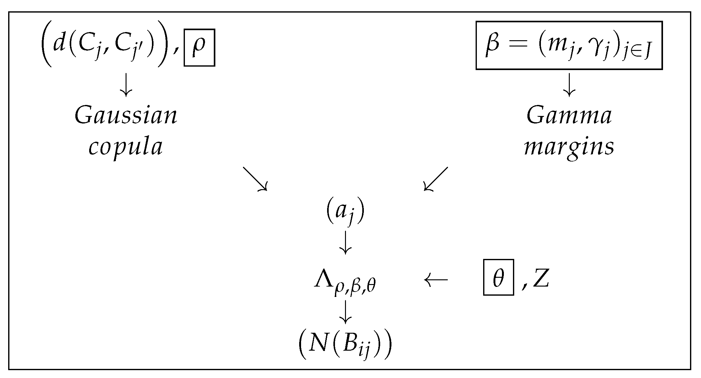
Proposition 5.
Let S be a sample verifying conditions (C1), (C2), and (C3). For the model defined by Equation (3), if ( A j ) j J follows a multivariate gamma distribution with joint density g parameterized by ( β , ρ ) and spatial correlation given by a copula density c, then the conditional likelihood on A j = a j , for S with respect to the counting measure N and ( θ , β , ρ ) is
L ( θ , β , ρ ) ; ( N ( B ) ) B S , ( a j ) j J = j J i = 1 n j ( a j S ν ( B i j , θ , Z ) ) N ( B i j ) N ( B i j ) ! exp ( a j S ν ( B i j , θ , Z ) ) c F A j ( a j ) j J j J f A j ( a j ) ,
where F A j is the cumulative distribution function of A j , and f A j is given by Equation (9). ρ stands for the copula density parameter.
Proof of Proposition 5. 
The joint density g is the product of the marginal densities multiplied by the copula density c. Consequently, g ( a j ) j J = c F A j ( a j ) j J j J f A j ( a j ) . Proposition 3 leads to the final result. □
In the case where the copula density is constant equal to 1, the A j are independent and expression (10) holds. In the sequel, we will use a multivariate gaussian copula [24] so that the correlation c o r ( A j , A j ) between two effects A j and A j depends on the distance d ( C j , C j ) between centroids:
u [ 0 , 1 ] n , c ( u ) = | W | 1 2 exp 1 2 ( u * ) t ( W 1 I n ) u * ,
where
u * = ( ϕ 1 ( u 1 ) , , ϕ 1 ( u n ) ) ,
ϕ 1 is the inverse of the standard normal probability distribution function, and
W = ρ d ( C j , C j ) ( j , j ) J 2 with ρ [ 0 , 1 ] .
The greater ρ is, the higher the dependency between effects is. The greater the distance is between C j and C j , the lower is the dependency between effects A j and A j .
Note that Lee [27] has shown that, in the case of a bivariate Gaussian copula with gamma margins, c o r ( A j , A j ) cannot be resolved analytically but numerically.

4. Statistical Inference on the Model Parameters

In this section, we consider again a set S of sampling units verifying conditions C1, C2 and C3 as defined in Section 3, and effects distributed according to the gamma law. We first focus on the case where the effects A j , j J , are independent and use likelihood techniques to estimate the model parameters. Then, the case of dependent A j is considered within a Bayesian framework.

4.1. Case of Independent Effects

When the effects A j are independent, the unconditional likelihood given by Equation (10) can be used to estimate the model parameters.
Proposition 6.
Let S be a sample verifying conditions (C1), (C2), and (C3). Assume the A j are independent and distributed according to Γ ( m j , γ j ) as defined by Equation (9). If θ is known, the maximum likelihood estimator for β = ( m j , γ j ) j J is such that:
m j ^ = y + j S ν + ( B j , θ , Z )
with y + j = i y i j and S ν + ( B j , θ , Z ) = i = 1 n j S ν ( B i j , θ , Z ) .
The estimator γ j ^ is obtained numerically from the following equation:
k = 0 y + j 1 1 γ j ^ + k + log γ j ^ y + j + γ j ^ = 0 .
Proof of Proposition 6.
The first order derivative of the log-likelihood log L ( θ , β ) ; ( N ( B ) ) B S given by Equation (10) with respect to parameter m j is as follows:
log L ( θ , β ) ; ( N ( B ) ) B S m j = γ j y + j m j γ j S ν + ( B j , θ , Z ) m j ( m j S ν + ( B j , θ , Z ) + γ j ) .
Solving the equation log L ( θ , β ) ; ( N ( B ) ) B S m j = 0 for m j gives:
m j ^ = y + j S ν + ( B j , θ , Z ) ,
with y + j = i y i j and S ν + ( B j , θ , Z ) = i = 1 n j S ν ( B i j , θ , Z ) .
The first order derivative of the log-likelihood log L ( θ , β ) ; ( N ( B ) ) B S with respect to parameter γ j is:
log L ( θ , β ) ; ( N ( B ) ) B S γ j = k = 0 y + j 1 1 γ j + k + log γ j m j S ν + ( B j , θ , Z ) + γ j + m j S ν + ( B j , θ , Z ) y + j m j S ν + ( B j , θ , Z ) + γ j .
By replacing m j and γ j with their maximum likelihood estimators, respectively, m j ^ and γ j ^ , we get the final equation:
k = 0 y + j 1 1 γ j ^ + k + log γ j ^ y + j + γ j ^ = 0 .
It is worth noticing that the maximum likelihood of γ j does not depend on θ . The following corollary gives us the maximum likelihood estimators when θ is unknown.
Corollary 5.
Under conditions (C1), (C2), and (C3), if the A j are independent and gamma-distributed, the maximum likelihood estimators for ( θ , β ) , where β = ( m j , γ j ) j J , are such that:
m j ^ = y + j S ν + ( B j , θ ^ , Z ) ,
with S ν + ( B j , θ ^ , Z ) = i = 1 n j S ν ( B i j , θ ^ , Z ) and θ ^ obtained from the following q equations:
j J i = 1 n j y i j S ν ( B i j , θ ^ , Z ) m j ^ S ν ( B i j , θ ^ , Z ) θ l = 0 , l = 1 , , q .
γ j ^ is obtained numerically from the same equation given in Proposition 6.
Proof of Corollary 5.
This is a straightforward consequence of Proposition 6. □
Corollary 6.
Under conditions (C1), (C2), and (C3), and regularity conditions, if the A j are independent and gamma-distributed, then the covariance matrix of ( β ^ , θ ^ ) is estimated by:
M ( β ^ , θ ^ ) = H m m 0 H m θ 0 H γ γ 0 H θ m 0 H θ θ 1 ,
where
H m m = d i a g E γ ^ j S ν + ( B j , θ ^ , Z ) y + j + γ ^ j j J , H γ γ = d i a g E k = 0 y + j 1 1 ( γ ^ j + k ) 2 y + j γ ^ j ( y + j + γ ^ j ) 2 j J ,
H θ θ = E 2 log L ( β ^ , θ ^ ) ; ( N ( B ) ) B S θ l θ s l , s a n d H m θ = E 2 log L ( θ ^ , β ^ ) ; ( N ( B ) ) B S m j θ l j , l .
Proof of Corollary 6.
Differentiating twice the negative log-likelihood function with respect to the model parameters, we get the Fisher information as the expectation of this Hessian matrix. By replacing β = ( m j , γ j ) j J and θ with their maximum likelihood estimators, respectively, β ^ and θ ^ in the second order derivatives, we get the final results. □

4.2. Case of Dependent Effects

When the A j are dependent, the unconditional likelihood in Equation (7) is analytically intractable. Since the A j are not observed, the conditional likelihood given by Equation (11) cannot be used directly for likelihood-based methods but rather within a Bayesian framework. For example, Lee [33] described implementations of spatial hierarchical models via simulation techniques. In fact, such MCMC methods provide tools for making inference about missing data and model parameters [29,34]. These MCMC techniques allow samples from the posterior distribution of ( β , θ , ρ , ( A j ) j J ) to be drawn and then the calculation of any statistic based on the parameters and unobserved effects. This posterior distribution is proportional to
L ( θ , β , ρ ) ; ( N ( B ) ) B S , ( a j ) j J × π ( θ ) π ( β ) π ( ρ ) ,
where π ( θ ) , π ( β ) , and π ( ρ ) are the prior distributions for θ , β , and ρ .
Therefore, we propose a hybrid Gibbs-Metropolis-Hasting algorithm based on an acyclic directed graph (Figure 1) which provides posterior distribution samples for θ , β , and ρ . An example of such MCMC applications was presented in Valmy and Vaillant [35].

5. Analysis of BLSD Data

We performed our analysis on a dataset from Martinique consisting of spatial counts of the BLSD, a major foliar disease of bananas. Preliminary results show that four strata could be considered on the basis of the average annual rainfall (Figure 2).
On the other hand, because of sampling cost and effort, data could not be collected over the whole island (Figure 3). The proportion of Cavendish plots was the only covariate considered in this analysis. In fact, Cavendish banana is the most susceptible cultivar to BLSD and is mainly grown for export.
Table 1 summarizes some information on the number of positive cases with BLSD observed in each sampling unit. The overdispersion is very significant in each stratum.
Samples from the parameter’s posterior distribution obtained by performing the MCMC procedure provide the estimates given in Table 2. From the 95% confidence intervals, we can deduce that the parameters ρ , ( m j , γ j ) j { 1 , 2 , 3 , 4 } are significantly different from zero at the 5% level. Only θ is not significantly different from zero which means that the proportion of Cavendish plot is not correlated to the number of positive cases. The m j distributions are significantly different from each other (p-value < 2.2 × 10 16 ) and this is also the case for the γ j distributions. The posterior distribution of ρ spreads over [0.03, 0.96] with a mode at 0.49 which implies a significant spatial dependency between strata. Note that the lower bound of the 95% posterior confidence interval for γ 4 is equal to exp ( 0.07 ) = 1.0725 . Therefore, parameter γ 4 is most likely greater than 1: the spatial effect in stratum 4 is significant.

6. Conclusions

We propose a model for spatial count data obtained from a stratified sampling in presence of overdispersion with spatial dependency built from a gaussian copula. Stratum random effects and spatial covariates can be considered and statistical inference can be performed within a Bayesian framework. Posterior samples of the model parameters are obtained by means of a hybrid Gibbs-Metropolis-Hasting algorithm. There are potential applications in various scientific fields, such as epidemiology and ecology. An illustration is given from data of Black Leaf Streak Disease (BLSD) on banana in Martinique. Differences from one stratum to another are significant, as well as their spatial dependency. A non-significant influence of proportion of Cavendish plots on the number of positive cases is found.

Author Contributions

W.O. and J.V. contributed equally to this work in conceptualization, methodology, software and original draft preparation. All authors have read and agreed to the published version of the manuscript.

Funding

This research was partly funded by the French Embassy in Haiti (grant 973355H).

Acknowledgments

We would like to thank DAAF and FREDON Martinique for providing the BLSD spatio-temporal data, Météo France for providing Martinique’s rainfall data, and the French Embassy in Haiti for partly funding Walguen Oscar’s PhD work.

Conflicts of Interest

The authors declare no conflict of interest.

References

  1. Brémaud, P. Point Processes and Queues: Martingale Dynamics; Springer: Berlin/Heidelberg, Germnay, 1981; Volume 50. [Google Scholar]
  2. Daley, D.J.; Vere-Jones, D. An Introduction to the Theory of Point Processes: Volume 1: Elementary Theory and Methods; Springer: New York, NY, USA; Berlin/Heidelberg, Germnay, 2003. [Google Scholar]
  3. Lánskỳ, P.; Vaillant, J. Stochastic model of the overdispersion in the place cell discharge. Biosystems 2000, 58, 27–32. [Google Scholar] [CrossRef]
  4. Møller, J.; Ghorbani, M.; Rubak, E. Mechanistic spatio-temporal point process models for marked point processes, with a view to forest stand data. Biometrics 2016, 72, 687–696. [Google Scholar] [CrossRef] [Green Version]
  5. Peng, R.D.; Schoenberg, F.P.; Woods, J.A. A space–time conditional intensity model for evaluating a wildfire hazard index. J. Am. Stat. Assoc. 2005, 100, 26–35. [Google Scholar] [CrossRef] [Green Version]
  6. Vaillant, J.; Puggioni, G.; Waller, L.A.; Daugrois, J. A spatio-temporal analysis of the spread of sugarcane yellow leaf virus. J. Time Ser. Anal. 2011, 32, 396–406. [Google Scholar] [CrossRef]
  7. Li, Z.; Cui, L.; Chen, J. Traffic accident modelling via self-exciting point processes. Reliab. Eng. Syst. Saf. 2018, 180, 312–320. [Google Scholar] [CrossRef]
  8. De Oliveira, V. Hierarchical Poisson models for spatial count data. J. Multivar. Anal. 2013, 122, 393–408. [Google Scholar] [CrossRef]
  9. Diggle, P.J.; Tawn, J.A.; Moyeed, R.A. Model-based geostatistics. J. R. Stat. Soc. Ser. C (Appl. Stat.) 1998, 47, 299–350. [Google Scholar] [CrossRef]
  10. Diggle, P.J. Statistical Analysis of Spatial and Spatio-Temporal Point Patterns; CRC Press: Boca Raton, FL, USA, 2014. [Google Scholar]
  11. Wakefield, J. Disease mapping and spatial regression with count data. Biostatistics 2007, 8, 158–183. [Google Scholar] [CrossRef] [PubMed]
  12. Ickstadt, K.; Wolpert, R.L. Spatial regression for marked point processes. Bayesian Stat. 1998, 6, 323–341. [Google Scholar]
  13. Cressie, N. Statistics for Spatial Data; John Wiley & Sons: Hoboken, NJ, USA, 2015. [Google Scholar]
  14. Sain, S.R.; Cressie, N. A spatial model for multivariate lattice data. J. Econom. 2007, 140, 226–259. [Google Scholar] [CrossRef]
  15. Ma, X.; Luan, S.; Du, B.; Yu, B. Spatial copula model for imputing traffic flow data from remote microwave sensors. Sensors 2017, 17, 2160. [Google Scholar] [CrossRef] [PubMed] [Green Version]
  16. Durocher, M.; Chebana, F.; Ouarda, T.B. On the prediction of extreme flood quantiles at ungauged locations with spatial copula. J. Hydrol. 2016, 533, 523–532. [Google Scholar] [CrossRef]
  17. Cox, D.R. Some statistical methods connected with series of events. J. R. Stat. Soc. Ser. B (Methodol.) 1955, 17, 129–157. [Google Scholar] [CrossRef]
  18. Møller, J.; Syversveen, A.R.; Waagepetersen, R.P. Log gaussian cox processes. Scand. J. Stat. 1998, 25, 451–482. [Google Scholar] [CrossRef]
  19. Moller, J.; Waagepetersen, R.P. Statistical Inference and Simulation for Spatial Point Processes; CRC Press: Boca Raton, FL, USA, 2004. [Google Scholar]
  20. Neyens, T.; Faes, C.; Molenberghs, G. A generalized Poisson-gamma model for spatially overdispersed data. Spat. Spatio-Temporal Epidemiol. 2012, 3, 185–194. [Google Scholar] [CrossRef]
  21. Wolpert, R.L.; Ickstadt, K. Poisson/gamma random field models for spatial statistics. Biometrika 1998, 85, 251–267. [Google Scholar] [CrossRef] [Green Version]
  22. Sharma, G. Pros and cons of different sampling techniques. Int. J. Appl. Res. 2017, 3, 749–752. [Google Scholar]
  23. Pascutto, C.; Wakefield, J.; Best, N.; Richardson, S.; Bernardinelli, L.; Staines, A.; Elliott, P. Statistical issues in the analysis of disease mapping data. Stat. Med. 2000, 19, 2493–2519. [Google Scholar] [CrossRef]
  24. Xue-Kun Song, P. Multivariate dispersion models generated from Gaussian copula. Scand. J. Stat. 2000, 27, 305–320. [Google Scholar] [CrossRef]
  25. Masarotto, G.; Varin, C. Gaussian copula marginal regression. Electron. J. Stat. 2012, 6, 1517–1549. [Google Scholar] [CrossRef]
  26. Krupskii, P.; Genton, M.G. Factor copula models for data with spatio-temporal dependence. Spat. Stat. 2017, 22, 180–195. [Google Scholar] [CrossRef] [Green Version]
  27. Lee, T. Multisite stochastic simulation of daily precipitation from copula modeling with a gamma marginal distribution. Theor. Appl. Climatol. 2018, 132, 1089–1098. [Google Scholar] [CrossRef]
  28. Aitchison, J.; Ho, C. The multivariate Poisson-log normal distribution. Biometrika 1989, 76, 643–653. [Google Scholar] [CrossRef]
  29. Smith, A.F.; Roberts, G.O. Bayesian computation via the Gibbs sampler and related Markov chain Monte Carlo methods. J. R. Stat. Soc. Ser. B (Methodol.) 1993, 55, 3–23. [Google Scholar] [CrossRef]
  30. Karlis, D.; Xekalaki, E. Mixed poisson distributions. Int. Stat. Rev./Rev. Int. Stat. 2005, 73, 35–58. [Google Scholar] [CrossRef]
  31. Kotz, S.; Balakrishnan, N.; Johnson, N.L. Continuous Multivariate Distributions, Volume 1: Models and Applications; John Wiley & Sons: Hoboken, NJ, USA, 2004. [Google Scholar]
  32. Rahayu, A.; Prastyo, D.D. Multivariate Gamma Regression: Parameter Estimation, Hypothesis Testing, and Its Application. Symmetry 2020, 12, 813. [Google Scholar] [CrossRef]
  33. Lee, D. CARBayes: An R package for Bayesian spatial modeling with conditional autoregressive priors. J. Stat. Softw. 2013, 55, 1–24. [Google Scholar] [CrossRef] [Green Version]
  34. Landry, C.; Abadie, C.; Bonnot, F.; Vaillant, J. A Spatio-temporal Stochastic Model for an Emerging Plant Disease Spread in a Heterogeneous Landscape. Int. J. Comput. Appl. 2021, 975, 1–7. [Google Scholar]
  35. Valmy, L.; Vaillant, J. Bayesian Inference on a Cox Process Associated with a Dirichlet Process. Int. J. Comput. Appl. 2014, 95, 1–7. [Google Scholar] [CrossRef]
Figure 1. Acyclic directed graph of the hierarchical model defined by Proposition 5.
Mathematics 09 00524 g001
Figure 2. Average annual precipitation in Martinique (from Météo France).
Mathematics 09 00524 g002
Figure 3. Available set of sampling units: black units are observed, grey units are not observed, white units are uncolonizable: high mountain and volcano (from Landry et al. (2021) [34]).
Mathematics 09 00524 g003
Table 1. Test of dispersion for the number of positive cases. n j , x ¯ j , s j 2 , I d j ^ are, respectively, the number of sampling units, the mean number of positive cases, the variance of the positive case number, the estimated index of dispersion in stratum j. The pvalue corresponds to the test of overdispersion.
Stratum j n j x ¯ j s j 2 I d j ^ p-Value
11501.212.802.32 0.0 × 10 0
2601.904.502.37 1.7 × 10 8
3701.134.724.18 0.0 × 10 0
4600.320.902.84 2.6 × 10 12
Table 2. Markov chain Monte Carlo (MCMC) posterior distribution results.
ParameterPosterior MeanPosterior Standard Deviation95% Posterior Confidence Interval
ρ 0.4860.28[0.03,0.96]
θ 5.215.21[−3.70,11.32]
log ( m 1 ) 1.941.19[−0.26,3.63]
log ( m 2 ) 1.570.61[0.26,2.70]
log ( m 3 ) 1.290.53[−0.07,2.08]
log ( m 4 ) 4.291.47[0.59,5.69]
log ( γ 1 ) −0.930.92[−2.56,0.70]
log ( γ 2 ) −0.670.74[−1.97,0.65]
log ( γ 3 ) 1.671.56[−0.55,4.48]
log ( γ 4 ) 5.863.40[0.07,11.14]
Publisher’s Note: MDPI stays neutral with regard to jurisdictional claims in published maps and institutional affiliations.

