Oriented Fuzzy Numbers vs. Fuzzy Numbers

Abstract

A formal model of an imprecise number can be given as, inter alia, a fuzzy number or oriented fuzzy numbers. Are they formally equivalent models? Our main goal is to seek formal differences between fuzzy numbers and oriented fuzzy numbers. For this purpose, we examine algebraic structures composed of numerical spaces equipped with addition, dot multiplication, and subtraction determined in a usual way. We show that these structures are not isomorphic. It proves that oriented fuzzy numbers and fuzzy numbers are not equivalent models of an imprecise number. This is the first original study of a problem of a dissimilarity between oriented fuzzy numbers and fuzzy numbers. Therefore, any theorems on fuzzy numbers cannot automatically be extended to the case of oriented fuzzy numbers. In the second part of the article, we study the purposefulness of a replacement of fuzzy numbers by oriented fuzzy numbers. We show that for a portfolio analysis, oriented fuzzy numbers are more useful than fuzzy numbers. Therefore, we conclude that oriented fuzzy numbers are an original and useful tool for modelling a real-world problems.

1. Introduction

An imprecise number is an approximation of a fixed value crisp number. A commonly accepted model of an imprecise number is a fuzzy number (FN) [1,2], determined as a fuzzy subset of the space of real numbers. The intuitive concept of ordered FN was introduced by Kosiński and his co-workers [3,4,5] as an extension of the FN concept. Ordered FNs’ usefulness follows from the fact that it is interpreted as FN equipped with information about the position of the approximated number. Ordered FNs have already begun to find their use in modelling a real-world problems [6,7,8,9,10,11,12,13,14,15,16,17,18,19].

Unfortunately, the ordered FNs’ theory has one significant drawback. Kosiński shows that there exist such ordered FNs that their sum cannot be represented by a membership function [20]. For this formal reason, the Kosiński’ theory was revised in [21] in this way that a new definition of ordered FNs corresponds to the intuitive definition by Kosiński. An Ordered FN defined in the context of the revised theory is now called an oriented FN (OFN) [22]. OFNs are already used in decision analysis, economics, and finance [23,24,25,26,27,28,29].

In the field of fuzzy sets, many authors propose such new concepts and theories that are isomorphic with the existing elements of the general theory of fuzzy sets [30]. Klement and Mesiar show a lot of such examples in their paper [30]. For this reason, they recommend an in-depth confrontation of the newly proposed concepts with the existing historically shaped elements of the fuzzy set theory. Finally, they emphasize that any modification of an existing fuzzy concept may be accepted if it is more useful in certain applications. The authors of this article fully agree with the postulates expressed by Klement and Mesiar.

The FN is a commonly accepted model of an imprecise number. In our work [21], we propose the concept of OFN as a new model of an imprecise number. Therefore, in line with Klement and Mesiar postulates [30], our main goal is to look for formal differences between the FN and OFN. To the best of our knowledge, it is the first study devoted to this problem. We will examine algebraic structures composed of numerical spaces equipped with addition and dot multiplication. In each considered case, subtraction is determined in a usual way. We will look here for an answer to the question of whether these structures are isomorphic. Moreover, at the end of the article, we will examine the advisability of replacing FNs by OFNs in the portfolio analysis. A negative answer to the first question and a positive solution to the other problem will confirm the fact that OFNs are an original and useful tool for modelling real-world problems.

Our paper is organized in a following way. Section 2 presents the concept of fuzzy sets defined as some extension of isomorphism between crisp sets and indicator functions. Section 3 briefly describes the idea of FNs. The arithmetic of FNs is presented. In Section 4, the original Kosiński’s theory of ordered FNs is discussed. The OFN notion is introduced in Section 5. The same chapter describes arithmetic operations on OFNs. In Section 6, the authors present results of their observations of differences between FNs and OFNs. Section 7 provides some suggestions for imprecision measures dedicated to OFNs. In Section 8, we consider imprecision measures determined for the case of trapezoidal OFNs. Section 9 describes the effects of replacing FNs by OFNs in portfolio analysis. Section 10 summarizes the main findings of our research and suggests some new directions of future investigation. Appendix A presents such modified notation of numerical intervals which is used in this paper.

2. Fuzzy Sets–Basic Facts

The space of all declarative sentences is noted by the symbol $\mathbb{P}$. Subjects of any cognitive-application activity are elements of a space $\mathbb{X}$. The basic tool for classifying these elements is the concept of a set. For any predicate ${\phi }_A:\mathbb{X}\to \mathbb{P}$, the set $A\subset \mathbb{X}$ can be determined in the following way

$$A=\left\{x\in \mathbb{X}: {\phi }_A\left(x\right),{\phi }_A\in {\mathbb{P}}^{\mathbb{X}} \right\}$$

(1)

The predicate ${\phi }_A\in {\mathbb{P}}^{\mathbb{X}}$ is called a predicate of the set $A\subset \mathbb{X}$. Any set and its predicate are one-to-one link. For unique determination of a set form, it is necessary to determine the manner in which the relationship between the actual state of affairs and the information contained in the sentence about this state is given.

The starting point for a discussion on this topic is to reduce our considerations to the classical propositional calculus. The subject of the classical propositional calculus are only those declarative sentences that are true or false. Any sentence that meet this condition is called a logical sentence. The space of all logical sentences is noted by the symbol ${\mathbb{P}}_0\subset \mathbb{P}$. For each true sentence $𝓅\in {\mathbb{P}}_0$, we assign the truth value

$$v\left(𝓅\right)=1$$

(2)

For each false sentence $𝓅\in {\mathbb{P}}_0$, we assign the truth value

$$v\left(𝓅\right)=0.$$

(3)

In this way, we define the function of a logical evaluation $v\in {\left\{0;1\right\}}^{{\mathbb{P}}_0}$. Any set

$$A=\left\{xϵ\mathbb{X}: {\phi }_A\left(x\right), {\phi }_A\in {\mathbb{P}}_0^{\mathbb{X}}\right\}$$

(4)

is a set (crisp set) described in the classical set theory. The family of all such sets is noted by the symbol $ℬ\left(\mathbb{X}\right)$. For any set $A\in ℬ\left(\mathbb{X}\right)$, we determine its characteristic function ${\chi }_A\in {\left\{0,1\right\}}^{\mathbb{X}}=2^{\mathbb{X}}$ given by the identity

$${\chi }_A\left(x\right)=v\left({\phi }_A\left(x\right)\right)$$

(5)

The characteristic function value ${\chi }_A\left(x\right)$ is equal to the truth value of the sentence $“x\in A”$.

Two-valued logic has been criticized many times. Therefore, it was extended by Łukasiewicz [31,32] to multivalued logic. The subject of considerations in multivalued logic are those sentences for which the connected relation “no less true” is uniquely defined. The space of all sentences meeting this condition is noted by the symbol ${\mathbb{P}}_1\subset \mathbb{P}$. We have ${\mathbb{P}}_0\subset {\mathbb{P}}_1\subset \mathbb{P}$. Using multivalued logic, we assume that:

• Any sentence is not less true than any false sentence,
• Any true sentence is not less true than any sentence.

For each sequence $𝓅\in {\mathbb{P}}_1$, we assign the truth value $\tilde{v}\left(𝓅\right)$ understood as a “degree in which the evaluated sentence is true”. Because multivalued logic is an extension of two-valued logic, for any sentence $𝓅\in {\mathbb{P}}_0$ we have

$$\tilde{v}\left(𝓅\right)=v\left(𝓅\right).$$

(6)

In this way, we define the function of logical evaluation $\tilde{v}\in {\left[0,1\right]}^{{\mathbb{P}}_1}$. Any set

$$A=\left\{xϵ\mathbb{X}: {\phi }_A\left(x\right), {\phi }_A\in {\mathbb{P}}_1^{\mathbb{X}}\right\}$$

(7)

is a fuzzy set intuitively introduced by Zadeh [33], Menger [34,35], and Klaua [36,37] (see [38]). We denote the family of all fuzzy sets by the symbol $ℱ\left(\mathbb{X}\right)$. For any fuzzy set $A\in ℱ\left(\mathbb{X}\right)$, we determine its membership function ${\mu }_A\in {\left[0,1\right]}^{\mathbb{X}}$ given by the identity

$${\mu }_A\left(x\right)=\tilde{v}\left({\phi }_A\left(x\right)\right).$$

(8)

The membership function value ${\mu }_A\left(x\right)$ is equal to the truth value of the sentence “$x\in A$”.

We can define any fuzzy set in a more formal way. The spaces $ℬ\left(\mathbb{X}\right)$ and $2^{\mathbb{X}}$ are isomorphic. This isomorphism is determined by the increasing bijection $\mathsf{\Phi }:2^{\mathbb{X}}\to ℬ\left(\mathbb{X}\right)$ i.e.,

$${\forall }_{{\chi }_A, {\chi }_B\in 2^{\mathbb{X}}} : {\chi }_A\le {\chi }_B\Rightarrow \mathsf{\Phi }\left({\chi }_A\right)\subset \Phi \left({\chi }_B\right).$$

(9)

Then we have

$$ℬ\left(\mathbb{X}\right)=\mathsf{\Phi }\left(2^{\mathbb{X}}\right).$$

(10)

It means that the family $ℬ\left(\mathbb{X}\right)$ of all crisp sets is determined by isomorphism $\mathsf{\Phi }$ as the image of the family $2^{\mathbb{X}}$ of all characteristic function on the space $\mathbb{X}$. Because $2^{\mathbb{X}}\subset {\left[0,1\right]}^{\mathbb{X}}$, we can extend the isomorphism $\mathsf{\Phi }:2^{\mathbb{X}}\to ℬ\left(\mathbb{X}\right)$ to an increasing injection $\tilde{\mathsf{\Phi }}$ determined on ${\left[0,1\right]}^{\mathbb{X}}$. For any membership function ${\mu }_A\in {\left[0,1\right]}^{\mathbb{X}}$, the value

$$A=\tilde{\mathsf{\Phi }}\left({\mu }_A\right)$$

(11)

is called a fuzzy set. Then, the space $ℱ\left(\mathbb{X}\right)$ is determined in the following way

$$ℱ\left(\mathbb{X}\right)=\tilde{\mathsf{\Phi }}\left({\left[0,1\right]}^{\mathbb{X}}\right)$$

(12)

Increasing bijection $\tilde{\mathsf{\Phi }}$ used above is not uniquely defined. The identity (8) shows that the unique form of the isomorphism depends on the type of multivalued logic used. On the other hand, this multivalued logic determines the set operators in $ℱ\left(\mathbb{X}\right)$. In our considerations, a set operators are determined in the following way

$${\mu }_{A{\displaystyle \cup }B}\left(x\right)={\mu }_A\left(x\right)\vee {\mu }_B\left(x\right)=\max \left\{{\mu }_A\left(x\right), {\mu }_B\left(x\right)\right\},$$

(13)

$${\mu }_{A{\displaystyle \cap }B}\left(x\right)={\mu }_A\left(x\right)\wedge {\mu }_B\left(x\right)=\min \left\{{\mu }_A\left(x\right), {\mu }_B\left(x\right)\right\},$$

(14)

$${\mu }_{A^C}\left(x\right)=1-{\mu }_A\left(x\right).$$

(15)

The development trends of fuzzy set theory are restricted by Zadeh’s extension principle [39,40,41]. This principle can be formally described as follows.

Let the fixed notion $\mathcal{Q}$ be explicitly defined with the use of two-valued logic as some relationship between elements of space $\mathbb{X}$. Then this notion is described by predicate ${\phi }_Q\in {\mathbb{P}}_0^{\mathbb{X}}$. Then Zadeh’s extension principle states that any extension $\tilde{\mathcal{Q}}$ of the notion $\mathcal{Q}$ in the fuzzy case is described by the same predictor ${\phi }_Q\in {\mathbb{P}}_1^{\mathbb{X}}$ evaluated with the use of multivalued logic.

Any fuzzy subset $A\in ℱ\left(\mathbb{X}\right)$ may be characterized using the following crisp sets:

• the $\alpha -$cuts ${\left[A\right]}_{\alpha }$ determined for each $\alpha \in \left[0,1\right]$ as follows

  $${\left[A\right]}_{\alpha }=\left\{x\in \mathbb{X}: {\mu }_A\left(x\right)\ge \alpha \right\},$$

  (16)
• the support closure ${\left[\mathcal{A}\right]}_{0^{+}}$ given in the following way

  $$\overline{\mathcal{S}𝓊𝓅}\left(A\right)={\left[A\right]}_{0^{+}}=\underset{\alpha \to 0^{+}}{\lim }{\left[A\right]}_{\alpha },$$

  (17)
• the core $\mathcal{C}ℴ𝓇𝓮\left(A\right)$ distinguished with the use of the formula

  $$\mathcal{C}ℴ𝓇𝓮\left(A\right)={\left[A\right]}_1=\left\{x\in \mathbb{X}: {\mu }_A\left(x\right)=1\right\}.$$

  (18)

3. Fuzzy Number–Basic Facts

An imprecise number may be considered as a family of real values belonging to it in a varying degree. For this reason, an imprecise number is usually represented by a FN defined as a fuzzy subset of the family $\mathbb{R}$ of all real numbers. The most general definition of FN was proposed by Dubois and Prade [1,2].

Definition 1.

The fuzzy number (FN) is such a fuzzy subset$ℒ\in ℱ\left(\mathbb{R}\right)$represented by its upper semi-continuous membership function${\mu }_L\in {\left[0,1\right]}^{\mathbb{R}}$satisfying the conditions:

$$\mathcal{C}ℴ𝓇𝓮(ℒ)\ne \varnothing ,$$

(19)

$${\forall }_{\left(x,y,z\right)\in {\mathbb{R}}^3}: x\le y\le z\Rightarrow {\mu }_L\left(y\right)\ge \min \left\{{\mu }_L\left(x\right),{\mu }_L\left(z\right)\right\},$$

(20)

$${\forall }_{\left(a,d\right)\in {\mathbb{R}}^2}: \overline{\mathcal{S}𝓊𝓅}\left(ℒ \right)=\left[a,d\right]$$

(21)

The set of all FN we denote by the symbol $\mathbb{F}$. Each FN $ℒ$ is interpreted as an imprecise number “about $z$” for any $z\in \mathcal{C}ℴ𝓇𝓮(ℒ)$. Understanding the phrase “about $z$” depends on the applied pragmatics of the natural language. Any real number $a\in \mathbb{R}$ is such FN $⟦a⟧\in \mathbb{F}$ that

$$\mathcal{C}ℴ𝓇𝓮(⟦a⟧)=\overline{\mathcal{S}𝓊𝓅}\left(⟦a⟧\right)=\left\{a\right\}.$$

(22)

It implies that $\mathbb{R}\subset \mathbb{F}$. On the other hand, any FN fulfilling (22) is a real number. Moreover, we immediately obtain from conditions (22) that any number $⟦a⟧$ is represented by its membership function ${\mu }_{⟦a⟧}\in {\left[0,1\right]}^{\mathbb{R}}$ given by the identity

$${\mu }_{⟦a⟧}\left(x\right)=\{\begin{array}{c}1 x=a,\\ 0 x\ne a.\end{array}$$

(23)

Let symbol $\ast$ denotes any arithmetic operation defined in $\mathbb{R}$. By symbol $⊛$ we denote an extension of arithmetic operation $\ast$ to $\mathbb{F}$. According to the Zadeh’s Extension Principle, for any pair $\left(\mathcal{K},ℒ\right)\in {\mathbb{F}}^2$ represented respectively by their membership functions ${\mu }_K,{\mu }_L\in {\left[0,1\right]}^{\mathbb{R}}$, Dubois and Prade [2] define the FN

$$ℳ=\mathcal{K}⊛ℒ$$

(24)

by means of its membership function ${\mu }_M\in {\left[0,1\right]}^{\mathbb{R}}$ given by the identity:

$${\mu }_M\left(z\right)=\sup \left\{\min \left\{{\mu }_K\left(x\right),{\mu }_L\left(y\right)\right\}: z=x\ast y,\left(x,y\right)\in \mathbb{R}\right\}.$$

(25)

In line with the above, we can extend basic arithmetic operators to a fuzzy case in a following way:

• For any pair $\left(\beta ,ℒ \right)\in \mathbb{R}\times \mathbb{F}$, the “dot multiplication”
  $$ℳ=\beta \odot ℒ$$

  (26)

  determined with the use of its membership function ${\mu }_M\in {\left[0,1\right]}^{\mathbb{R}}$ given by the identity

  $${\mu }_M\left(z\right)=\sup \left\{{\mu }_L\left(y\right): z=\beta ·y\in \mathbb{R}\right\};$$

  (27)
• For any pair $\left(\mathcal{K},ℒ\right)\in {\mathbb{F}}^2$, the “addition”
  $$ℳ=\mathcal{K}\oplus ℒ$$

  (28)

  determined with the use of its membership function ${\mu }_M\in {\left[0,1\right]}^{\mathbb{R}}$ given by the identity

  $${\mu }_M\left(z\right)=\sup \left\{\min \left\{{\mu }_K\left(x\right),{\mu }_L\left(y\right)\right\}: z=x+y,\left(x,y\right)\in {\mathbb{R}}^2\right\}.$$

  (29)

In this article, we will discuss an algebraic structure $\langle \mathbb{F},\odot ,\oplus \rangle$ understood as the space $\mathbb{F}$ equipped with dot multiplication $\odot$ and addition $\oplus$. From the identity (29) we get that the addition $\oplus$ is associative and commutative. Moreover, we have

Lemma 1.

The number$⟦0⟧$is the additive identity (The additive identity is also sometimes called an additive neutral element) in the algebraic structure$\langle \mathbb{F},\odot ,\oplus \rangle$.

Proof of Lemma 1.

Let us take any FN$ℒ\in \mathbb{F}$represented by its membership function${\mu }_L\in {\left[0,1\right]}^{\mathbb{R}}$. The identities (23) and (29) imply that the sum

$$ℳ=⟦0⟧\oplus ℒ$$

(30)

is represented by its membership function${\mu }_M\in {\left[0,1\right]}^{\mathbb{R}}$given as follows

$${\mu }_M\left(z\right)=\sup \left\{\min \left\{{\mu }_{⟦0⟧}\left(x\right),{\mu }_L\left(y\right)\right\}: z=x+y,\left(x,y\right)\in {\mathbb{R}}^2\right\}=\min \left\{{\mu }_{⟦0⟧}\left(0\right),{\mu }_L\left(z\right)\right\}={\mu }_L\left(z\right).$$

This together with the addition commutativity proves that

$$⟦0⟧\oplus ℒ=ℒ\oplus ⟦0⟧=ℒ.$$

(31)

□.

For the algebraic structure $\langle \mathbb{F},\odot ,\oplus \rangle$, we can determine following operators:

• The unary minus operator $“–”$ on $\mathbb{R}$ extended to the minus operator $\ominus$ on $\mathbb{F}$ by the identity

$$\ominus ℒ=\left(-1\right)\odot ℒ,$$

(32)

• The subtraction $“–”$ on $\mathbb{R}$ extended to the subtraction $\ominus$ on $\mathbb{F}$ by the identity

$$\mathcal{K}\ominus ℒ=\mathcal{K}\oplus \left(\ominus ℒ\right).$$

(33)

The unary minus operator $\ominus$ and the subtraction $\ominus$ meet the condition (25) of Dubois and Prade definition.

Equations (25) and (29) are very difficult to apply. A great facilitation here is the fact that any FN can be equivalently defined as follows:

Theorem 1 [42].

For any FN$ℒ$there exists such a non-decreasing sequence$\left(a,b,c,d\right) \subset \mathbb{R}$that$ℒ\left(a,b,c,d,L_L,R_L\right)=ℒ\in ℱ\left(\mathbb{R}\right)$determined by its membership function${\mu }_L\left(·|a,b,c,d,L_L,R_L\right)\in {\left[0,1\right]}^{\mathbb{R}}$given as follows

$${\mu }_L\left(·|a,b,c,d,L_L,R_L\right)=\{\begin{array}{cc}0\hfill & x\notin [a,d]\\ L_L\left(x\right)\hfill & x\in [a,b[\\ 1\hfill & x\in [b,c]\\ R_L\left(x\right)\hfill & x\in ]c,d]\end{array}$$

(34)

where the left reference function$L_L\in {\left[0,1\right]}^{\left[a,b\right]}$and the right reference function$R_L\in {\left[0,1\right]}^{\left[c,d\right]}$are upper semi-continuous monotonic ones meeting the condition (21).

In further considerations, we will use the following concepts.

Definition 2.

For any upper semi-continuous non-decreasing function$L\in {\left[0, 1\right]}^{\left[u, v\right]}$, its cut-function$L^{\star }\in {\left[u,v\right]}^{\left[0;1\right]}$is determined by the identity

$$L^{\star }\left(\alpha \right)=\min \left\{x\in \left[u,v\right]: L\left(x\right)\ge \alpha \right\}.$$

(35)

Definition 3.

For any upper semi-continuous non-increasing function$R\in {\left[0, 1\right]}^{\left[u, v\right]}$its cut-function$R^{\star }\in {\left[u,v\right]}^{\left[0,1\right]}$is determined by the identity

$$R^{\star }\left(\alpha \right)=\max \left\{x\in \left[u,v\right]: R\left(x\right)\ge \alpha \right\}.$$

(36)

Definition 4.

For any bounded continuous and non-decreasing function$l\in {\left[l\left(0\right), l\left(1\right)\right]}^{\left[0,1\right]}$its pseudo inverse$l^{⊲}\in {\left[0,1\right]}^{\left[l\left(0\right), l\left(1\right)\right]}$is determined by the identity

$$l^{⊲}\left(x\right)=\max \left\{\alpha \in \left[0,1\right]:l\left(\alpha \right)=x\right\}.$$

(37)

Definition 5.

For any bounded continuous and non-increasing function$r\in {\left[r\left(1\right), r\left(0\right)\right]}^{\left[0,1\right]}$its pseudo inverse$r^{⊲}\in {\left[0;1\right]}^{\left[r\left(1\right), r\left(0\right)\right]}$is determined by the identity

$$r^{⊲}\left(x\right)=\min \left\{\alpha \in \left[0,1\right]:r\left(\alpha \right)=x\right\}.$$

(38)

Using results obtained in [43], for any pair $\left(ℒ\left(a,b,c,d,L_K,R_K\right),ℒ\left(e,f,g,h,L_M,R_M\right)\right)\in {\mathbb{F}}^2$ we get the sum

$$ℒ\left(a,b,c,d,L_K,R_K\right)\oplus ℒ\left(e,f,g,h,L_M,R_M\right)=ℒ\left(a+e,b+f,c+g,d+h,L_J,R_J\right),$$

(39)

where

$${\forall }_{\alpha \in \left[0,1\right]} l_J\left(\alpha \right)=L_K^{\star }\left(\alpha \right)+L_M^{\star }\left(\alpha \right),$$

(40)

$${\forall }_{\alpha \in \left[0,1\right]} r_J\left(\alpha \right)=R_K^{\star }\left(\alpha \right)+R_M^{\star }\left(\alpha \right),$$

(41)

$${\forall }_{x\in \left[a+e,b+f\right]} L_J\left(x\right)=l_J^{⊲}\left(x\right),$$

(42)

$${\forall }_{x\in \left[c+g,d+h\right]} R_J\left(x\right)=r_J^{⊲}\left(x\right).$$

(43)

In an analogous way, for any pair $\left(\beta ,ℒ\left(a,b,c,d,L_K,R_K\right)\right)\in \mathbb{R}\times \mathbb{F}$ we get the dot product

$$\beta \odot ℒ\left(a,b,c,d,L_K,R_K\right)=\{\begin{array}{c}L\left(\beta ·a,\beta ·b,\beta ·c,\beta ·d,L_W,R_W\right), \beta \ge 0,\\ L\left(\beta ·d,\beta ·c,\beta ·b,\beta ·a,R_W,L_W\right), \beta <0.\end{array}$$

(44)

where

$${\forall }_{\alpha \in \left[0,1\right]} l_W\left(\alpha \right)=\beta ·L_K^{\star }\left(\alpha \right),$$

(45)

$${\forall }_{\alpha \in \left[0,1\right]} r_W\left(\alpha \right)=\beta ·R_K^{\star }\left(\alpha \right),$$

(46)

$${\forall }_{x\in \left[\beta ·a,\beta ·b\right]} L_W\left(x\right)=l_W^{⊲}\left(x\right),$$

(47)

$${\forall }_{x\in \left[\beta ·c,\beta ·d\right]} R_W\left(x\right)=r_W^{⊲}\left(x\right).$$

(48)

Example 1.

Let us calculate the dot product

$$\mathcal{W}=\left(-3\right)\odot \mathcal{K},$$

(49)

where the FN$\mathcal{K}=ℒ\left(2,4,8,10,L_K,R_k\right)$is characterized by its membership function

$${\mu }_K\left(x\right)=\left\{\begin{array}{cc}0\hfill & x\notin [2,10]\\ L_K\left(x\right)\hfill & x\in [2,4[\\ 1\hfill & x\in [4,8]\\ R_K\left(x\right)\hfill & x\in ]8,10]\end{array}\right\}=\{\begin{array}{cc}0\hfill & x\notin [2,10]\\ \frac{2x-4}{x}\hfill & x\in [2,4[\\ 1\hfill & x\in [4,8]\\ \frac{3x-30}{x-14}\hfill & x\in ]8,10]\end{array}$$

(50)

It is very easy to check that reference functions $L_K$ and $R_K$ are strictly monotonic. Using dependences (44)–(48), we get

$$\mathcal{W}=ℒ\left(-3·10,-3·8,-3·4,-3·2,R_W,L_W\right)=\overleftrightarrow{ℒ}\left(-30,-24,-12,-6,R_W,L_W\right),$$

(51)

where

$$L_K^{\star }\left(\alpha \right)=\min \left\{x\in \left[2,14\right]: L_K\left(x\right)\ge \alpha \right\}=L_K^{-1}\left(\alpha \right)=\frac{4}{2-\alpha }$$

(52)

$$R_K^{\star }\left(\alpha \right)=\max \left\{x\in \left[8,10\right]: R_K\left(x\right)\ge \alpha \right\}=R_K^{-1}\left(\alpha \right)=\frac{14\alpha -30}{\alpha -3}$$

(53)

$$l_W\left(\alpha \right)=3·\frac{4}{2-\alpha }=\frac{12}{2-\alpha },$$

(54)

$$r_W\left(\alpha \right)=3·\frac{14\alpha -30}{\alpha -3}=\frac{42\alpha -90}{\alpha -3},$$

(55)

$$L_W\left(x\right)=\max \left\{\alpha \in \left[0;1\right]:\frac{12}{2-\alpha }=x\right\}=\frac{2x-12}{x},$$

(56)

$$R_W\left(x\right)=\min \left\{\alpha \in \left[0;1\right]:\frac{42\alpha -90}{\alpha -3}=x\right\}=\frac{3·x-90}{x-42}$$

(57)

Example 2.

Let us calculate the sum

$$\mathcal{J}=\mathcal{K}\oplus ℳ,$$

(58)

where FN$\mathcal{K}$is characterized by its membership function (50) and FN$ℳ=ℒ\left(5,6,11,15,L_M,R_M\right)$is determined by membership function

$${\mu }_M\left(x\right)=\left\{\begin{array}{cc}0\hfill & x\notin [5,15]\\ L_M\left(x\right)\hfill & x\in [5,6[\\ 1\hfill & x\in [6,11]\\ R_M\left(x\right)\hfill & x\in ]11,15]\end{array}\right\}=\{\begin{array}{cc}0\hfill & x\notin [5,15]\\ \frac{3x-15}{x-3}\hfill & x\in [5,6[\\ 1\hfill & x\in [6,11]\\ \frac{3x-45}{x-23}\hfill & x\in ]11,15]\end{array}$$

(59)

In addition, reference functions $L_M$ and $R_M$ are strictly monotonic. Using dependences (39)–(43), we get

$$\mathcal{J}=ℒ\left(2+5,4+6,8+11,10+15,L_J,R_J\right)=\overleftrightarrow{ℒ}\left(7,10,19,25,L_J,R_J\right),$$

(60)

where

$$L_M^{\star }\left(\alpha \right)=\min \left\{x\in \left[5,6\right]: L_M\left(x\right)\ge \alpha \right\}=L_M^{-1}\left(\alpha \right)=\frac{3\alpha -15}{\alpha -3},$$

(61)

$$R_M^{\star }\left(\alpha \right)=\max \left\{x\in \left[11,15\right]: R_M\left(x\right)\ge \alpha \right\}=R_M^{-1}\left(\alpha \right)=\frac{23\alpha -45}{\alpha -3}$$

(62)

$$l_J\left(\alpha \right)=\frac{4}{2-\alpha }+\frac{3\alpha -15}{\alpha -3}=\frac{\left(3\alpha -7\right)\left(\alpha -6\right)}{\left(\alpha -2\right)\left(\alpha -3\right)},$$

(63)

$$r_J\left(\alpha \right)=\frac{14\alpha -30}{\alpha -3}+\frac{23\alpha -45}{\alpha -3}=\frac{37\alpha -75}{\alpha -3},$$

(64)

$$\begin{gathered} L_J\left(x\right)=\max \left\{\alpha \in \left[0;1\right]:\frac{\left(3\alpha -7\right)\left(\alpha -6\right)}{\left(\alpha -2\right)\left(\alpha -3\right)}=x\right\}=\max \left\{\frac{\sqrt{x^2-10·x+121}+5·x-25}{2·x-6},\frac{\sqrt{x^2-10·x+121}-5·x+25}{2·x-6} \right\}= \\ =\frac{\sqrt{x^2-10·x+121}+5·x-25}{2·x-6}, \end{gathered}$$

(65)

$$R_J\left(x\right)=\min \left\{\alpha \in \left[0;1\right]:\frac{37\alpha -75}{\alpha -3}=x\right\}=\frac{3·x-75}{x-37}$$

(66)

Example 2 shows a very high level of formal complexity of any FNs addition. Therefore, in many applications researchers limit their considerations to the following kind of FNs.

Definition 6.

For any nondecreasing sequence$\left(a,b,c,d\right)\subset \mathbb{R}$, the trapezoidal fuzzy number (TrFN) is the FN$Tr\left(a,b,c,d\right)=\mathcal{T}\in \mathbb{F}$determined explicitly by its membership functions${\mu }_T\in {\left[0,1\right]}^{\mathbb{R}}$as follows

$${\mu }_T\left(x\right)={\mu }_{Tr}\left(x|a,b,c,d\right)=\{\begin{array}{c} 0 x\notin \left[a,d\right]\\ \frac{x-a}{b-a} x\in \left[a,b\right[\\ 1 x\in \left[b,c\right]\\ \frac{x-d}{c-d} x\in \left]c,d\right]\end{array}$$

(67)

The space of all TrFNs is denoted by the symbol ${\mathbb{F}}_{Tr}$. For any $a\in \mathbb{R}$ The TrFN we have

$$Tr\left(a,a,a,a\right)=⟦a⟧.$$

(68)

Therefore, we can write $\mathbb{R}\subset {\mathbb{F}}_{Tr}\subset \mathbb{F}$.

Using identities (39)–(43), for any pair $\left(Tr\left(a,b,c,d\right),Tr\left(e,f,g,h\right)\right)\in {\mathbb{F}}_{Tr}^2$ we get the sum

$$Tr\left(a,b,c,d\right)\oplus Tr\left(e,f,g,h\right)=Tr\left(a+e,b+f,c+g,d+h\right).$$

(69)

Using identities (44)–(48), for any pair $\left(\beta ,Tr\left(a,b,c,d\right)\right)\in \mathbb{R}\times {\mathbb{F}}_{Tr}$ we get the dot product

$$\beta \odot Tr\left(a,b,c,d\right)=\{\begin{array}{c}Tr\left(\beta ·a,\beta ·b,\beta ·c,\beta ·d\right), \beta \ge 0,\\ Tr\left(\beta ·d,\beta ·c,\beta ·b,\beta ·a\right), \beta <0.\end{array}$$

(70)

Using identities (33), (69), and (70) for any pair $\left(Tr\left(a,b,c,d\right),Tr\left(e,f,g,h\right)\right)\in {\mathbb{F}}_{Tr}^2$ we get the subtraction

$$Tr\left(a,b,c,d\right)\oplus Tr\left(e,f,g,h\right)=Tr\left(a-h,b-g,c-f,d-e\right).$$

(71)

The main disadvantage of FN arithmetic is described by lemma below.

Lemma 2.

The subtraction$\ominus$is not an inverse operator to addition$\oplus$.

Proof of Lemma 2.

Let us take into account TrFN$Tr\left(a,b,c,d\right)\notin \mathbb{R}$. In accordance with (23), we have$a<d$. Using (71), we get

$$\begin{gathered} Tr\left(a,b,c,d\right)\ominus Tr\left(a,b,c,d\right)=Tr\left(a,b,c,d\right)\oplus \left(\ominus Tr\left(a,b,c,d\right)\right)= \\ =Tr\left(a,b,c,d\right)\oplus Tr\left(-d,-c,-b,-a\right)=Tr\left(a-d,b-c,c-b,d-a\right)\ne ⟦0⟧ \end{gathered}$$

(72)

because of$a-d<d-a$. □

This raises problems concerning the solution of fuzzy linear equations and with the interpretation of specific improper fuzzy arithmetic results.

4. Kosiński’s Theory

The notion of ordered FN is intuitively introduced by Kosiński and his co-writers [3,4,5] as such a model of an imprecise number and its arithmetic that subtraction is the inverse operator to addition. Kosiński was going to define ordered FN as an extension of a concept of FN. The original definition of ordered FNs was formulated in the following way.

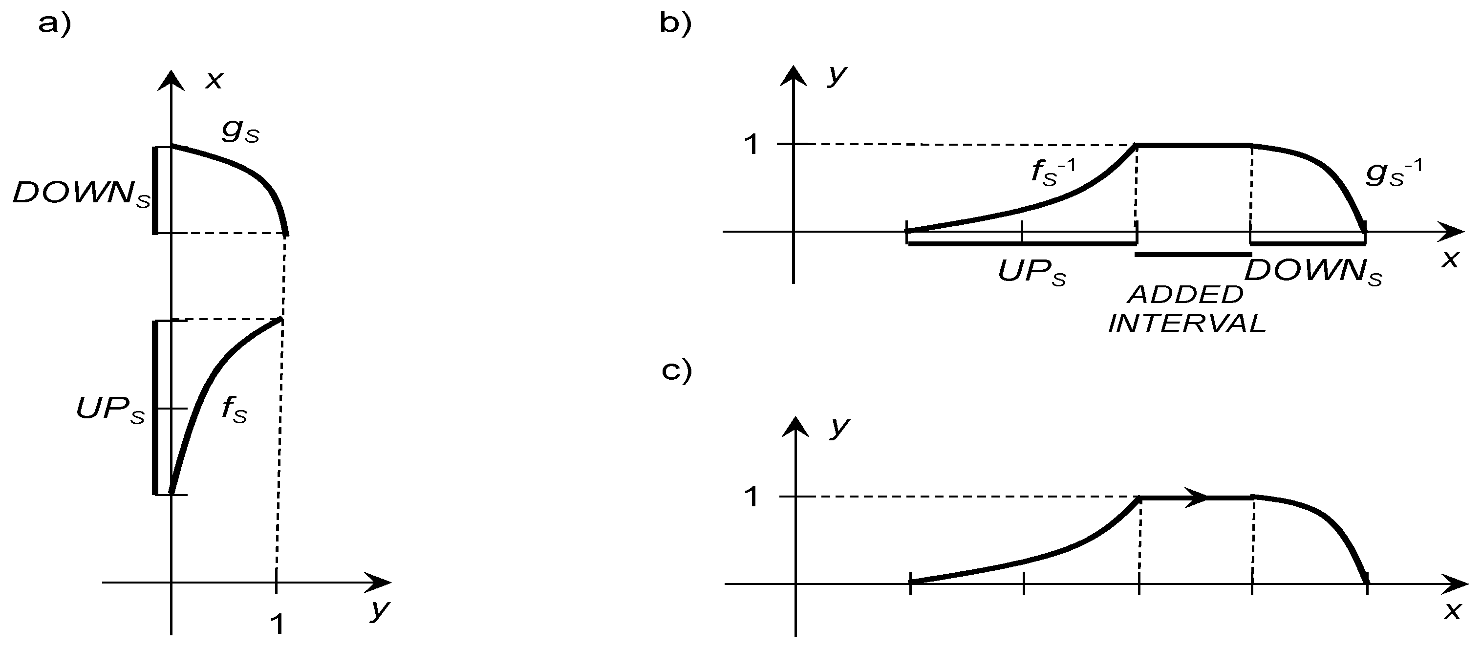
Definition 7.

For any sequence$\left(a,b,c,d\right)\subset \mathbb{R}$, the ordered FN$\stackrel{=}{\mathcal{S}}\left(a,b,c,d,f_s,g_s\right)$is an ordered pair$\left(f_S,g_S\right)$of continuous bijections$f_S:\left[0,1\right]\to U{P}_S=\left[a,b\right]\ne \left[a,a\right]$and$g_S:\left[0,1\right]\to DOW{N}_S=\left[c,d\right]\ne \left[d,d\right]$fulfilling the condition:

$$f_s\left(0\right)=a \wedge f_s\left(1\right)=b \wedge g_s\left(1\right)=c \wedge g_s\left(0\right)=d$$

(73)

For any ordered FN $\stackrel{=}{\mathcal{S}}\left(a,b,c,d,f_s,g_s\right)$ the function $f_S:\left[0,1\right]\to U{P}_S$ is called an up-function. Then the function $g_S:\left[0,1\right]\to DOW{N}_S$ is called a down-function.

In Definition 7, Kosiński assumed implicitly the monotonicity of the sequence $\left(a,b,c,d\right)\subset \mathbb{R}$. He has marked this condition on the graphs only. Some example of such Kosiński’s graphs are presented in Figure 1a. Using additional assumption, Kosiński stated that the ordered FN $\stackrel{=}{\mathcal{S}}\left(a,b,c,d,f_s,g_s\right)$ determine the FN $ℒ\left(a,b,c,d,f_s^{-1},g_s^{-1}\right)=ℒ$ determined with the use of its membership function ${\mu }_L\left(·|a,b,c,d,f_s^{-1},g_s^{-1}\right)\in {\left[0,1\right]}^{\mathbb{R}}$ given by the identity (34). An example of a graph of such FN is shown in Figure 1b.

By ${\boxed{\ast }}_K$ we denote an extension of an arithmetic operation $\ast$ defined on $\mathbb{R}$ to the space of all ordered FN. For any pair $\left(\stackrel{=}{\mathcal{S}}\left(a,b,c,d,f_K,g_K\right),\stackrel{=}{\mathcal{S}}\left(e,f,g,h,f_L,g_L\right) \right)$ of ordered FNs, Kosiński defines extension ${\boxed{\ast }}_K$ in a following way

$$\stackrel{=}{\mathcal{S}}\left(a,b,c,d,f_K,g_K\right){\boxed{\ast }}_K\stackrel{=}{\mathcal{S}}\left(e,f,g,h,f_L,g_L\right)=\stackrel{=}{\mathcal{S}}\left(a\ast e,b\ast f,c\ast g,d\ast h,f_K\ast f_L,g_K\ast g_L\right)$$

(74)

In the Kosiński’s theory, definition (74) replaces definition (25) proposed by Dubois and Prade [2]. Kosiński has developed his theory without using the results obtained by Goetschel and Voxman [43]. Nevertheless, the Kosiński’s definition of addition is coherent with identity (29) describing addition $\oplus$ of FNs.

Any sequence $\left(a,b,c,d\right)\subset \mathbb{R}$ meets exactly one of the following conditions

$$b<c \vee (b=c \wedge a<d),$$

(75)

$$b>c \vee (b=c \wedge a>d),$$

(76)

$$a=b=c=d.$$

(77)

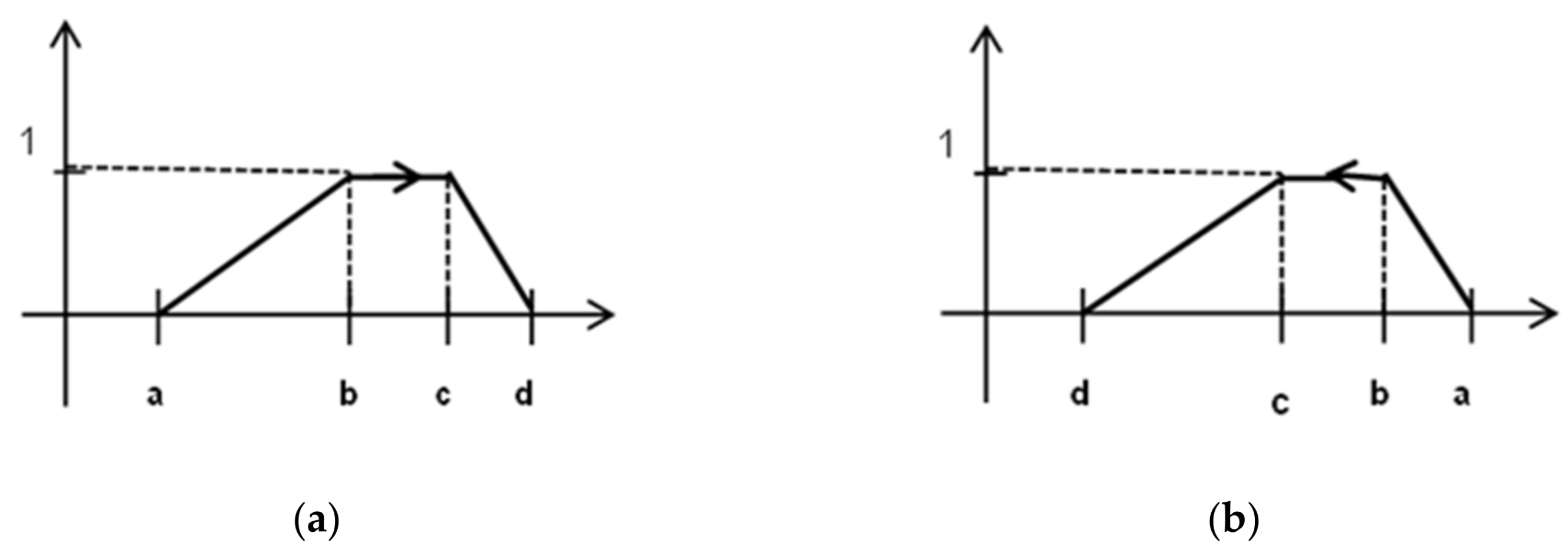
If the condition (75) is fulfilled then the ordered FN $\stackrel{=}{\mathcal{S}}\left(a,b,c,d,f_s,g_s\right)$ is positively oriented. For this case, some examples of graphs of Kosiński’s maps are presented in Figure 1a. The graph of FN $ℒ\left(a,b,c,d,f_s^{-1},g_s^{-1}\right)$ membership function with a positive orientation is shown in Figure 1c. This graph has an arrow denoting the orientation, which provides additional information. A positively oriented ordered FN is interpreted as an imprecise number, which may increase. Some example of membership function of FN determined by a positively oriented ordered FN is presented in Figure 2a.

If the condition (76) is fulfilled then the ordered FN $\stackrel{=}{\mathcal{S}}\left(a,b,c,d,f_s,g_s\right)$ is negatively oriented. A negatively oriented ordered FN is interpreted as such an imprecise number, which may decrease. Some example of a membership function of FN determined by a negatively oriented ordered FN is presented in the Figure 2b.

If the condition (77) is fulfilled then the ordered FN $\stackrel{=}{\mathcal{S}}\left(a,b,c,d,f_s,g_s\right)$ is not related to any FN. This disadvantage of original Kosiński’s theory will be discussed below.

If the sequence $\left(a,b,c,d\right)\subset \mathbb{R}$ is not monotonic then using the identity (34) we get the membership relation ${\mu }_L\left(·|a,b,c,d,f_s^{-1},g_s^{-1}\right)\subset \mathbb{R}\times \left[0,1\right]$, which is not a function. Therefore, this relation cannot be considered as a membership function of any fuzzy set. For this reason, for any non-monotonic sequence $\left(a,b,c,d\right)\subset \mathbb{R}$ the ordered FN $\stackrel{=}{\mathcal{S}}\left(a,b,c,d,f_s,g_s\right)$ is called an improper one [4]. Some example of a membership relation determined by a negatively oriented improper ordered FN is presented in Figure 3. The remaining ordered FNs are called proper ones. Some examples of proper ordered FNs are presented in Figure 2.

We note above that for the case (77), the ordered FN $\stackrel{=}{\mathcal{S}}\left(a,b,c,d,f_s,g_s\right)$ is undefined. We can remove the disadvantage by means of the generalization of Kosiński’s theory to the case when an up-function and a down-function are monotonic continuous surjections. Thanks to the use of Goetschel–Voxman results [43], we can generalize the ordered FN theory in such a manner that fully corresponds to the intuitive Kosiński’s approach to the notion of ordered FN. We agree with other scientists [13,15] that the ordered FN should be called the Kosiński’s number. For this reason, the generalized ordered FN will be called Kosiński’s numbers.

Definition 8.

For any sequence$\left(a,b,c,d\right)\subset \mathbb{R}$, the Kosiński’s number (KN)$\stackrel{=}{\mathcal{S}}\left(a,b,c,d,f_s,g_s\right)$is an ordered pair$\left(f_S,g_S\right)$of continuous monotonic surjections$f_S:\left[0,1\right]\to U{P}_S=\left[a,b\right]$and$g_S:\left[0,1\right]\to DOW{N}_S=\left[c,d\right]$fulfilling the condition (73).

In [21], it is shown that we have:

Theorem 2.

For any sequence$\left(a,b,c,d\right)\subset \mathbb{R}$, the KN$\stackrel{=}{\mathcal{S}}\left(a,b,c,d,f_s,g_s\right)$is explicitly determined by its membership relation${\mu }_s\left(·|a,b,c,d,f_s^{⊲}, g_s^{⊲}\right)\subset \mathbb{R}\times \left[0,1\right]$given by the identity

$${\mu }_L\left(x|a,b,c,d,f_s^{⊲}, g_s^{⊲}\right)=\{\begin{array}{cc}0\hfill & x\notin [a,d]\equiv [d,a]\\ f_s^{⊲}\left(x\right)\hfill & x\in [a,b[\equiv ]b,a]\\ 1\hfill & x\in [b,c]=[c,b]\\ g_s^{⊲}\left(x\right)\hfill & x\in ]c,d]\equiv [d,c[\end{array}$$

(78)

In Theorem 2, we use a modified notation of numerical intervals, which is explained in Appendix A. The space of all KN is denoted by the symbol $\check{\mathbb{K}}$. Any KN $\stackrel{=}{\mathcal{S}}\left(a,b,c,d,f_s,g_s\right)$ fulfilling the condition (75) is positively oriented. Any KN $\stackrel{=}{\mathcal{S}}\left(a,b,c,d,f_s,g_s\right)$ fulfilling the condition (76) is negatively oriented. Any KN $\stackrel{=}{\mathcal{S}}\left(d,d,d,d,f_s,g_s\right)$ is an unoriented FN $⟦d⟧\in \mathbb{F}$ fulfilling the condition (22). Then, we have identities

$$f_s\left(\alpha \right)=g_s\left(\alpha \right)=d.$$

(79)

Of course, then KN represents the crisp number $d\in \mathbb{R}$.

Let symbol $\ast$ denote any arithmetic operation defined in $\mathbb{R}$. By ${\boxed{\ast }}_K$ we denote an extension of arithmetic operation $\ast$ to $\check{\mathbb{K}}$. In the Kosiński’s theory, the arithmetic operations ${\boxed{\ast }}_K$ are defined by (74). In this way we obtain Kosiński’s arithmetic.

Using (74), for any pair $\left(\beta ,\stackrel{=}{\mathcal{S}}\left(a,b,c,d,f_s,g_s\right)\right)\in \mathbb{R}\times \check{\mathbb{K}}$ we get dot product

$$\beta {⊡}_K\stackrel{=}{\mathcal{S}}\left(a,b,c,d,f_s,g_s\right)=\stackrel{=}{\mathcal{S}}\left(\beta ·a,\beta ·b,\beta ·c,\beta ·d,\beta ·f_s,\beta ·g_s\right)$$

(80)

Comparing (44) with (80), we notice that the dot product $\odot$ and the dot product ${⊡}_K$ are different arithmetic operations. It implies that the Dubois–Prade definition (25) and the Kosiński’s definition (74) are not equivalent.

In an analogous way, for any pair $\left(\stackrel{=}{\mathcal{S}}\left(a,b,c,d,f_K,g_K\right),\stackrel{=}{\mathcal{S}}\left(e,f,g,h,f_L,g_L\right)\right)\in {\check{\mathbb{K}}}^2$ we get the sum

$$\stackrel{=}{\mathcal{S}}\left(a,b,c,d,f_K,g_K\right){⊞}_K\stackrel{=}{\mathcal{S}}\left(e,f,g,h,f_L,g_L\right)=\stackrel{=}{\mathcal{S}}\left(a+e,b+f,c+g,d+h,f_K+f_L,g_K+g_L\right).$$

(81)

The condition (74) implies that the unary operator minus ${\boxminus }_K$ and the subtraction ${\boxminus }_K$ may by expressed for $\check{\mathbb{K}}$ in the same way as for $\mathbb{F}$. Kosiński [20] has shown that:

• The addition ${⊞}_K$ is commutative and associative,
• The number $⟦0⟧$ is additive identity in the algebraic structure $\langle \check{\mathbb{K}}, {⊡}_K, {⊞}_K\rangle$,
• The subtraction ${\boxminus }_K$ is inverse operator to addition ${⊞}_K$.

Therefore, we can say that KNs fulfil the postulates put formulated by Kosiński. It is important advantages of Kosiński’s theory. On the other hand, let us look at the following example.

Example 3.

We add proper KNs$\left(\stackrel{=}{\mathcal{S}}\left(2,4,8,10,f_K,g_K\right),\stackrel{=}{\mathcal{S}}\left(15,11,6,5,f_L,g_L\right)\right)\in {\check{\mathbb{K}}}^2$, where

$$f_K\left(\alpha \right)=2·\alpha +2,$$

(82)

$$g_K\left(\alpha \right)=-2·\alpha +10,$$

(83)

$$f_L\left(\alpha \right)=-4·\alpha +15,$$

(84)

$$g_L\left(\alpha \right)=\alpha +5.$$

(85)

Using (81), we get

$$\stackrel{=}{ℳ}=\stackrel{=}{\mathcal{S}}\left(2,4,8,10,f_K,g_K\right){⊞}_K\stackrel{=}{\mathcal{S}}\left(15,11,6,5,f_L,g_L\right)=\stackrel{=}{\mathcal{S}}\left(17,15,14,15,f_M,g_M\right),$$

where

$$f_M\left(\alpha \right)=-2·\alpha +17,$$

(86)

$$g_M\left(\alpha \right)=-\alpha +15.$$

(87)

The KN $\stackrel{=}{ℳ}$ is an improper one because the sequence $\left(17,15,14,15\right)$ is not monotonic.

The above example shows that the sum of proper KNs may be an improper KN. This fact was already known to Kosiński [20].

On the other hand, this property of addition ${⊞}_K$ results in the fact that the improper KNs cannot be omitted from the Kosiński theory. This is a major inconvenience because improper numbers cannot be interpreted in the context of the fuzzy set theory. Such an assessment of the Kosinski theory indicates the need of revision.

5. Oriented Fuzzy Numbers

Under the influence of the above argumentation, Kosinski’s theory was revised in [21]. In the revised theory, KNs are replaced by a following kind of ordered FNs.

Definition 9 [21].

For any monotonic sequence$\left(a,b,c,d\right)\subset \mathbb{R}$, the oriented fuzzy number (OFN)$\overleftrightarrow{ℒ}\left(a,b,c,d,S_L,E_L\right)=\overleftrightarrow{ℒ}$is the pair of the orientation$\overrightarrow{a,d}=\left(a,d\right)$and FN$ℒ\in \mathbb{F}$determined with the use of its membership function${\mu }_L\left(\cdot |a,b,c,d,S_L,E_L\right)\in {\left[0,1\right]}^{\mathbb{R}}$given by (78), where the starting function$S_L\in {\left[0,1\right]}^{\left[a,b\right]}$and the ending function$E_L\in {\left[0,1\right]}^{\left[c,d\right]}$are upper semi-continuous monotonic ones meeting the condition (21).

The symbol $\mathbb{K}$ denotes the space of all OFNs. Theorem 2 shows that $\mathbb{K}\subset \check{\mathbb{K}}$. All OFNs are proper KNs. Any OFN represents an imprecise number equipped with information about the position of the approximated number. This information is expressed by an orientation of OFN. If $a<d$ then OFN $\overleftrightarrow{ℒ}\left(a,b,c,d,S_L,E_L\right)$ has the positive orientation $\overrightarrow{a,d}$. For any $z\in \left[b,c\right],$ the positively oriented OFN $\overleftrightarrow{ℒ}\left(a,b,c,d,S_L,E_L\right)$ is interpreted as an imprecise number “about or slightly above $z$”. By symbol ${\mathbb{K}}^{+}$ we denote the space of all positively oriented OFNs. If $a>d$, then OFN $\overleftrightarrow{ℒ}\left(a,b,c,d,S_L,E_L\right)$ has the negative orientation $\overrightarrow{a,d}$. For any $z\in \left[c,b\right],$ the negatively oriented TrOFN $\overleftrightarrow{ℒ}\left(a,b,c,d,S_L,E_L\right)$ is interpreted as an imprecise number “about or slightly below $z$”. By symbol ${\mathbb{K}}^{-}$ we denote the space of all negatively oriented OFNs. Understanding the phrases “about or slightly above $z$” and “about or slightly below $z$” depends on the used language pragmatics. If $a=d$, OFN $\overleftrightarrow{ℒ}\left(a,a,a,a,S_L,E_L\right)=⟦a⟧$ represents the number $a\in \mathbb{R}$, which is unoriented. All above facts imply that

$${\mathbb{K}}^{+}{\displaystyle \cup }\mathbb{R}{\displaystyle \cup }{\mathbb{K}}^{-}=\mathbb{K}\subset \check{\mathbb{K}}.$$

(88)

Let symbol $\ast$ denote any arithmetic operation defined in $\mathbb{R}$. By the symbol $\boxed{\ast }$ we denote an extension of arithmetic operation $\ast$ to $\mathbb{K}$. In the revised theory, the arithmetic operations $\boxed{\ast }$ are defined by

$$\overleftrightarrow{ℒ}\left(a_K,b_K,c_K,d_K,S_K,E_K\right)\boxed{\ast } \overleftrightarrow{ℒ}\left(a_M,b_M,c_M,d_M,S_M,E_M\right)=\overleftrightarrow{ℒ}\left(a_J,b_J,c_J,d_J,S_J,E_J\right),$$

(89)

where we have

$${\check{a}}_J=a_K\ast a_M,$$

(90)

$$b_J=b_K\ast b_M,$$

(91)

$$c_J=c_K\ast c_M,$$

(92)

$${\check{d}}_J=d_K\ast d_M,$$

(93)

$$a_J=\{\begin{array}{c}\min \left\{{\check{a}}_J,b_J\right\}, \left(b_J<c_J\right)\vee \left(b_J=c_J\wedge {\check{a}}_J\le {\check{d}}_J\right),\\ \max \left\{{\check{a}}_J,b_J\right\}, \left(b_J>c_J\right)\vee \left(b_J=c_J\wedge {\check{a}}_J>{\check{d}}_J\right),\end{array}$$

(94)

$$d_J=\{\begin{array}{c}\max \left\{{\check{d}}_J,c_J\right\}, \left(b_J<c_J\right)\vee \left(b_J=c_J\wedge {\check{a}}_J\le {\check{d}}_J\right),\\ \min \left\{{\check{d}}_J,c_J\right\}, \left(b_J>c_J\right)\vee \left(b_J=c_J\wedge {\check{a}}_J>{\check{d}}_J\right),\end{array}$$

(95)

$${\forall }_{\alpha \in \left[0;1\right]} s_J\left(\alpha \right)=\{\begin{array}{c}{S}_K^{\star }\left(\alpha \right)\ast S_M^{\star }\left(\alpha \right), a_J\ne b_J,\\ b_J, a_J=b_J.\end{array}$$

(96)

$${\forall }_{\alpha \in \left[0;1\right]} e_J\left(\alpha \right)=\{\begin{array}{c}{E}_K^{\star }\left(\alpha \right)\ast E_M^{\star }\left(\alpha \right), c_J\ne d_J,\\ c_J, c_J=d_J.\end{array}$$

(97)

$${\forall }_{x\in \left[a_J,b_J\right]} S_J\left(x\right)=s_J^{⊲}\left(x\right),$$

(98)

$${\forall }_{x\in \left[c_J,d_J\right]} E_J\left(x\right)=e_J^{⊲}\left(x\right).$$

(99)

In this way, we obtain the revised arithmetic. Theorem 2 implies that

$${\forall }_{\left(\overleftrightarrow{\mathcal{K}},\overleftrightarrow{ℳ}\right)\in {\mathbb{K}}^2}: \overleftrightarrow{\mathcal{K}}{\boxed{\ast }}_K\overleftrightarrow{ℳ}\in \mathbb{K}\Rightarrow \overleftrightarrow{\mathcal{K}}\boxed{\ast }\overleftrightarrow{ℳ}=\overleftrightarrow{\mathcal{K}}{\boxed{\ast }}_K\overleftrightarrow{ℳ}.$$

(100)

It means that the revised arithmetic does not change proper results obtained with the use of Kosiński’s arithmetic. In other cases, results obtained with the use of revised arithmetic are the best approximation of results obtained with the use of Kosinski’s arithmetic [21].

Using (89), for any pair $\left(\overleftrightarrow{ℒ}\left(a_K,b_K,c_K,d_K,S_K,E_K\right),\overleftrightarrow{ℒ}\left(a_M,b_M,c_M,d_M,S_M,E_M\right)\right)\in {\mathbb{K}}^2$ we get their sum

$$\overleftrightarrow{ℒ}\left(a_K,b_K,c_K,d_K,S_K,E_K\right)⊞\overleftrightarrow{ℒ}\left(a_M,b_M,c_M,d_M,S_M,E_M\right)=\overleftrightarrow{ℒ}\left(a_J,b_J,c_J,d_J,S_J,E_J\right),$$

(101)

where we have

$${\check{a}}_J=a_K+a_M,$$

(102)

$$b_J=b_K+b_M,$$

(103)

$$c_J=c_K+c_M,$$

(104)

$${\check{d}}_J=d_K+d_M,$$

(105)

$$a_J=\{\begin{array}{c}\min \left\{{\check{a}}_J,b_J\right\}, \left(b_J<c_J\right)\vee \left(b_J=c_J\wedge {\check{a}}_J\le {\check{d}}_J\right),\\ \max \left\{{\check{a}}_J,b_J\right\}, \left(b_J>c_J\right)\vee \left(b_J=c_J\wedge {\check{a}}_J>{\check{d}}_J\right),\end{array}$$

(106)

$$d_J=\{\begin{array}{c}\max \left\{{\check{d}}_J,c_J\right\}, \left(b_J<c_J\right)\vee \left(b_J=c_J\wedge {\check{a}}_J\le {\check{d}}_J\right),\\ \min \left\{{\check{d}}_J,c_J\right\}, \left(b_J>c_J\right)\vee \left(b_J=c_J\wedge {\check{a}}_J>{\check{d}}_J\right),\end{array}$$

(107)

$${\forall }_{\alpha \in \left[0;1\right]} s_J\left(\alpha \right)=\{\begin{array}{c}{S}_K^{\star }\left(\alpha \right)+S_M^{\star }\left(\alpha \right), a_J\ne b_J,\\ b_J, a_J=b_J.\end{array}$$

(108)

$${\forall }_{\alpha \in \left[0;1\right]} e_J\left(\alpha \right)=\{\begin{array}{c}{E}_K^{\star }\left(\alpha \right)+E_M^{\star }\left(\alpha \right), c_J\ne d_J,\\ c_J, c_J=d_J.\end{array}$$

(109)

$${\forall }_{x\in \left[a_J,b_J\right]} S_J\left(x\right)=s_J^{⊲}\left(x\right),$$

(110)

$${\forall }_{x\in \left[c_J,d_J\right]} E_J\left(x\right)=e_J^{⊲}\left(x\right).$$

(111)

In an analogous way, for any pair $\left(\beta ,\overleftrightarrow{ℒ}\left(a,b,c,d,S_K,E_K\right)\right)\in \mathbb{R}\times \mathbb{K}$ we get the dot product

$$\beta ⊡\overleftrightarrow{ℒ}\left(a,b,c,d,S_K,E_K\right)=\overleftrightarrow{ℒ}\left(\beta ·a,\beta ·b,\beta ·c,\beta ·d,S_W,E_W\right),$$

(112)

where

$${\forall }_{\alpha \in \left[0,1\right]} s_W\left(\alpha \right)=\beta ·S_K^{\star }\left(\alpha \right),$$

(113)

$${\forall }_{\alpha \in \left[0,1\right]} e_W\left(\alpha \right)=\beta ·E_K^{\star }\left(\alpha \right),$$

(114)

$${\forall }_{x\in \left[\beta ·a,\beta ·b\right]} S_W\left(x\right)=s_W^{⊲}\left(x\right),$$

(115)

$${\forall }_{x\in \left[\beta ·c,\beta ·d\right]} E_W\left(x\right)=e_W^{⊲}\left(x\right).$$

(116)

Example 4.

Let us calculate the dot product

$$\overleftrightarrow{\mathcal{W}}=\left(-3\right)⊡\overleftrightarrow{\mathcal{K}}$$

where the OFN$\overleftrightarrow{\mathcal{K}}=\overleftrightarrow{ℒ}\left(2,4,8,10,L_K,R_k\right)$is characterized by its membership function (50). Using dependences (112)–(116), we get

$$\overleftrightarrow{\mathcal{W}}=\overleftrightarrow{ℒ}\left(-3·2,-3·4,-3·8,-3·10,L_W,R_W\right)=\overleftrightarrow{ℒ}\left(-6,-12,-24,-30,L_W,R_W\right),$$

where the starting function$L_W$and ending function$R_W$are given respectively by (56) and (57).

Example 5.

Let us calculate the sum

$$\overleftrightarrow{\mathscr{H}}=\overleftrightarrow{\mathcal{K}}⊞\overleftrightarrow{\mathcal{N}},$$

(117)

where the OFN$\overleftrightarrow{\mathcal{K}}=\overleftrightarrow{ℒ}\left(2,4,8,10,L_K,R_k\right)$is determined by its membership function (50) and the OFN$\overleftrightarrow{\mathcal{N}}=\overleftrightarrow{ℒ}\left(15,11,6,5,R_M,L_M\right)$where the functions$R_M$ and $L_M$ are given by (59). Using dependences (102)–(107), we get

$${\check{a}}_J=2+15=17,$$

(118)

$$b_J=4+11=15,$$

(119)

$$c_J=8+6=14,$$

(120)

$${\check{d}}_J=10+5=15,$$

(121)

$$a_J=\left(\begin{array}{c}\min \left\{17,15\right\}, \left(15<14\right)\vee \left(15=14\wedge 17\le 15\right),\\ \max \left\{17,15\right\}, \left(15>14\right)\vee \left(15=14\wedge 17>15\right),\end{array}\right)=17,$$

(122)

$$d_J=\left(\begin{array}{c}\max \left\{15,14\right\}, \left(15<14\right)\vee \left(15=14\wedge 17\le 15\right),\\ \min \left\{15,14\right\}, \left(15>14\right)\vee \left(15=14\wedge 17>15\right),\end{array}\right)=14.$$

(123)

Therefore, using (101) and (108–111) we get

$$\overleftrightarrow{\mathscr{H}}=\overleftrightarrow{ℒ}\left(17,15,14,14,S_H,E_H\right),$$

(124)

where the functions $L_K^{\star }$ and $R_M^{\star }$ are given, respectively, by (52) and (62) and we have

$$s_H\left(\alpha \right)= L_K^{\star }\left(\alpha \right)+ L_K^{\star }\left(\alpha \right)=\frac{4}{2-\alpha }+\frac{23\alpha -45}{\alpha -3}=-\frac{23{\alpha }^2-95\alpha +102}{\left(2-\alpha \right)\left(\alpha -3\right)},$$

(125)

$$\begin{gathered} S_H\left(x\right)=\min \left\{\alpha \in \left[0;1\right]:-\frac{23{\alpha }^2-95\alpha +102}{\left(2-\alpha \right)\left(\alpha -3\right)}=x\right\}= \\ =\min \left\{\frac{\sqrt{x^2+10x-359}-5x+95}{46-2x},\frac{\sqrt{x^2+10x-359}+5x-95}{46-2x} \right\}=\frac{\sqrt{x^2+10x-359}+5x-95}{46-2x}, \end{gathered}$$

(126)

$$E_H\left(x\right)=1.$$

(127)

We note that the above determined arithmetic operations on OFNs and analogous operations on FN are quite different. Nevertheless, in an analogous way, we can determine following operators:

• The unary minus operator $“–”$ on $\mathbb{R}$ extended to the minus operator $\boxminus$ on $\mathbb{K}$ by the identity

  $$\boxminus \overleftrightarrow{ℒ}=\left(-1\right)⊡\overleftrightarrow{ℒ},$$

  (128)
• The subtraction $“–”$ on $\mathbb{R}$ extended to the subtraction $\boxminus$ on $\mathbb{K}$ by the identity

  $$\overleftrightarrow{\mathcal{K}}\boxminus \overleftrightarrow{ℒ}=\overleftrightarrow{\mathcal{K}}⊞(\boxminus \overleftrightarrow{ℒ}).$$

  (129)

The unary minus operator $\boxminus$ and the subtraction $\ominus$ meet the condition (89–99) of the revised definition.

Lemma 3.

The number$⟦0⟧$is the additive identity in the algebraic structure$\langle \mathbb{K}, ⊡, ⊞\rangle$.

Proof of Lemma 3.

The OFN$⟦0⟧$is explicitly represented by its membership function given as follows

$${\mu }_L\left(x|0,0,0,0,S_0,E_0\right)=\{\begin{array}{cc}0\hfill & x\notin [0,0]\\ S_0\left(x\right)\hfill & x\in [0,0[\\ 1\hfill & x\in [0,0]\\ E_0\left(x\right)\hfill & x\in ]0,0]\end{array}$$

(130)

where the starting function$S_0\in {\left[0,1\right]}^{\left[0,0\right]}$and the ending function$E_0\in {\left[0,1\right]}^{\left[0,0\right]}$are determined in the following way

$$S_0\left(0\right)=E_0\left(0\right)=1.$$

(131)

Then from (35) or (36), we get

$${\forall }_{\alpha \in \left[0,1\right]} : S_0^{\ast }\left(\alpha \right)=E_0^{\ast }\left(\alpha \right)=0.$$

(132)

Let us take into account any OFN$\overleftrightarrow{\mathcal{K}}=\overleftrightarrow{ℒ}\left(a,b,c,d,S_K,E_K\right)$. Then we have

$$\begin{gathered} \overleftrightarrow{\mathcal{W}}=\overleftrightarrow{\mathcal{K}}⊞⟦0⟧=\overleftrightarrow{ℒ}\left(a,b,c,d,S_K,E_K\right)⊞\overleftrightarrow{ℒ}\left(0,0,0,0,S_0,E_0\right)= \\ =\overleftrightarrow{ℒ}\left(a,b,c,d,S_W,E_W\right)=\overleftrightarrow{ℒ}\left(a,b,c,d,S_K,E_k\right) \end{gathered}$$

(133)

and due to (108–111) we obtain

$${\forall }_{\alpha \in \left[0;1\right]} s_W\left(\alpha \right)=S_K^{\star }\left(\alpha \right)+S_0^{\star }\left(\alpha \right)=S_K^{\star }\left(\alpha \right),$$

(134)

$${\forall }_{\alpha \in \left[0;1\right]} e_W\left(\alpha \right)=E_K^{\star }\left(\alpha \right)+E_0^{\star }\left(\alpha \right)=E_K^{\star }\left(\alpha \right),$$

(135)

$${\forall }_{x\in \left[a,b\right]} S_W\left(x\right)=s_W^{⊲}\left(x\right)=S_K\left(x\right),$$

(136)

$${\forall }_{x\in \left[c,d\right]} E_W\left(x\right)=e_W^{⊲}\left(x\right)=E_K\left(x\right).$$

(137)

□.

Lemma 4.

The subtraction$\boxminus$is an inverse operator to addition$⊞$.

Proof of Lemma 4.

Let us take into account any OFN$\overleftrightarrow{\mathcal{K}}=\overleftrightarrow{ℒ}\left(a,b,c,d,S_K,E_K\right)$. Then using (131), (112), and (101) we have

$$\begin{gathered} \overleftrightarrow{\mathcal{W}}=\overleftrightarrow{\mathcal{K}}\boxminus \overleftrightarrow{\mathcal{K}}=\overleftrightarrow{ℒ}\left(a,b,c,d,S_K,E_K\right)⊞\overleftrightarrow{ℒ}\left(-a,-b,-c,-d,-S_K,-E_K\right)= \\ =\overleftrightarrow{ℒ}\left(0,0,0,0,S_0,E_0\right)=⟦0⟧, \end{gathered}$$

(138)

where the starting function$S_0\in {\left[0,1\right]}^{\left[0,0\right]}$and the ending function$E_0\in {\left[0,1\right]}^{\left[0,0\right]}$are determined by (133). □

Example 5 shows a very high level of formal complexity of any OFNs addition. Therefore, in many applications, researchers limit their considerations to the following kind of OFNs.

Definition 10 [21].

For any monotonic sequence$\left(a,b,c,d\right)\subset \mathbb{R}$, TrOFN$\overleftrightarrow{Tr}\left(a,b,c,d\right)=\overleftrightarrow{\mathcal{T}}$is OFN$\overleftrightarrow{\mathcal{T}}\in \mathbb{K}$determined explicitly by its membership functions${\mu }_T\in {\left[0,1\right]}^{\mathbb{R}}$as follows

$${\mu }_T\left(x\right)={\mu }_{Tr}\left(x|a,b,c,d\right)=\{\begin{array}{c} 0 x\notin \left[a,d\right]\equiv \left[d,a\right]\\ \frac{x-a}{b-a} x\in \left[a, b\right[\equiv \left]a,b\right]\\ 1 x\in \left[b,c\right]\equiv \left[c,b\right]\\ \frac{x-d}{c-d} x\in \left]c,d\right]\equiv \left[c,d\right[\end{array}$$

(139)

The symbol ${\mathbb{K}}_{Tr}$ denotes the space of all TrOFNs. The space of all positively oriented TrOFNs is denoted by the symbol ${\mathbb{K}}_{Tr}^{+}$. The space of all negatively oriented TrOFNs we denote by the symbol ${\mathbb{K}}_{Tr}^{-}$. TrOFN $\overleftrightarrow{Tr}\left(a,a,a,a\right)=⟦a⟧$ represents a crisp number $a\in \mathbb{R}$, which is unoriented. Summing up, all above facts imply that

$${\mathbb{K}}_{Tr}={\mathbb{K}}_{Tr}^{+}{\displaystyle \cup }\mathbb{R}{\displaystyle \cup }{\mathbb{K}}_{Tr}^{-}.$$

(140)

For any pair $\left(\overleftrightarrow{Tr}\left(a,b,c,d\right),\overleftrightarrow{Tr}\left(p-a,q-b,r-c,s-d\right)\right)\in {\mathbb{K}}_{Tr}^2$, the identities (101–111) imply that their sum is given as follows

$$\begin{gathered} \overleftrightarrow{Tr}\left(a,b, c,d\right)⊞\overleftrightarrow{Tr}\left(p-a,q-b, r-c,s-d\right)= \\ =\{\begin{array}{c}\overleftrightarrow{Tr}\left(\min \left\{p,q\right\},q, r,\max \left\{r,s\right\}\right), \left(q<r\right)\vee \left(q=r\wedge p\le s\right), \\ \overleftrightarrow{Tr}\left(\max \left\{p,q\right\},q, r,\min \left\{r,s\right\}\right), \left( q>r\right)\vee \left(q=r\wedge p>s\right).\end{array} \end{gathered}$$

(141)

The identity (112) implies that for any pair $\left(\beta ,\overleftrightarrow{Tr}\left(a,b,c,d\right)\right)\in \mathbb{R}\times {\mathbb{K}}_{Tr}$ we get the dot product

$$\beta ⊡\overleftrightarrow{Tr}\left(a,b,c,d\right)=\overleftrightarrow{Tr}\left(\beta ·a,\beta ·b,\beta ·c,\beta ·d\right).$$

(142)

It is very easy to check that if $\left(\overleftrightarrow{Tr}\left(a,b,c,d\right),\overleftrightarrow{Tr}\left(e,f,g,h\right)\right)\in {\mathbb{K}}_{Tr}^{+}\times {\mathbb{K}}_{Tr}^{+}{\displaystyle \cup }{\mathbb{K}}_{Tr}^{-}\times {\mathbb{K}}_{Tr}^{-}$ then the sequence $\left(a+e,b+f,c+g,d+h\right)$ is monotonic. This together with (143) implies that

$$\overleftrightarrow{Tr}\left(a,b, c,d\right)⊞\overleftrightarrow{Tr}\left(e,f, g,h\right)=\overleftrightarrow{Tr}\left(a+e,b+f, c+g,d+h\right).$$

(143)

When we compare the above relationship with (69), then for any pair $\left(\overleftrightarrow{Tr}\left(a,b,c,d\right),\overleftrightarrow{Tr}\left(e,f,g,h\right)\right)\in {\mathbb{K}}_{Tr}^{+}\times {\mathbb{K}}_{Tr}^{+}{\displaystyle \cup }{\mathbb{K}}_{Tr}^{-}\times {\mathbb{K}}_{Tr}^{-}$ we get

$$\begin{gathered} \overleftrightarrow{Tr}\left(a,b, c,d\right)⊞\overleftrightarrow{Tr}\left(e,f, g,h\right)=Tr\left(a+e,b+f, c+g,d+h\right)= \\ =Tr\left(a,b, c,d\right)\oplus Tr\left(e,f, g,h\right). \end{gathered}$$

(144)

6. Oriented Fuzzy Numbers Arithmetic vs. Fuzzy Numbers Arithmetic

Let us compare the algebraic structure $\langle \mathbb{F}, \odot , \oplus \rangle$ determined by (27) and (29) with the algebraic structure $\langle \mathbb{K}, ⊡, ⊞\rangle$ determined by (112) and (101).

For the algebraic structure $\langle \mathbb{F}, \odot , \oplus \rangle$ we can conclude as follows:

• From the identity (29), we immediately get that that the addition $\oplus$ is associative and commutative,
• Lemma 1 shows that the number $⟦0⟧$ is the additive identity,
• Lemma 2 shows that the subtraction $\ominus$ is not an inverse operator to addition $\oplus$.

For the algebraic structure $\langle \mathbb{K}, ⊡, ⊞\rangle$ we conclude:

• From the identity (101), we immediately get that that the addition $⊞$ is commutative,
• In [21] it is proved that the addition $⊞$ is not associative,
• Lemma 3 shows that the number $⟦0⟧$ is the additive identity,
• Lemma 4 shows that the subtraction $\boxminus$ is an inverse operator to addition $⊞$.

The above comparison shows that algebraic structures $\langle \mathbb{F}, \odot , \oplus \rangle$ and $\langle \mathbb{K}, ⊡, ⊞\rangle$ are not isomorphic. Therefore, OFNs and FNs should be considered as a different models of imprecision numbers. For this reason, any theorem on FNs cannot be automatically applied to OFNs.

On the other hand, we have the following nice relationship between FNs and OFNs. Let us consider the mapping $\mathcal{U}:\mathbb{K}\to \mathbb{K}$ given by identity

$$\mathcal{U}\left(\overleftrightarrow{ℒ}\left(a,b,c,d,S_L,E_L\right)\right)=\overleftrightarrow{ℒ}\left(d,c,b,a,E_L,S_L\right)$$

(145)

For this mapping we have:

$$\overleftrightarrow{ℒ}\in {\mathbb{K}}^{+}\Rightarrow \mathcal{U}\left(\overleftrightarrow{ℒ}\right)\in {\mathbb{K}}^{-},$$

(146)

$$\overleftrightarrow{ℒ}\in {\mathbb{K}}^{-}\Rightarrow \mathcal{U}\left(\overleftrightarrow{ℒ}\right)\in {\mathbb{K}}^{+},$$

(147)

$$\overleftrightarrow{ℒ}\in \mathbb{R}\Rightarrow \mathcal{U}\left(\overleftrightarrow{ℒ}\right)=\overleftrightarrow{ℒ}.$$

(148)

We see that the mapping (147) is such axial symmetry on the space $\mathbb{K}$ that the symmetry axis is equal to the $\mathbb{R}$. Moreover, Theorem 1 and Definition 9 imply that the space $\mathbb{F}$ and the space ${\mathbb{K}}^{+}{\displaystyle \cup }\mathbb{R}$ are isomorphic. This fact together with (149) and (150) proves that the space $\mathbb{K}$ is a symmetry closure of the space $\mathbb{F}$.

7. Evaluation of Imprecision for Oriented Fuzzy Numbers

After Klir [44] we understand information imprecision as a superposition of ambiguity and indistinctness of information. Ambiguity is understood as a lack of an explicit recommendation one alternative among various others. Indistinctness is interpreted as a lack of a clear distinction between recommended and not recommended alternatives.

The increase in an OFN ambiguity causes a higher number of recommended alternatives. This results in an increase in the risk of choosing an incorrect alternative from recommended ones. This may cause one to make a decision, which will result in the loss of chances ex post. The possibility of such an event is called the ambiguity risk. Therefore, the increase in the ambiguity of OFN implies the increase in ambiguity risk. The right tool for measuring the OFN ambiguity is an extension of energy measure $𝓭\in {\left[{\mathbb{R}}_0^{+}\right]}^{\mathbb{F}}$ defined for FNs by de Luca and Termini [45].

For any FN $ℒ=L\left(a,b,c,d,L_L,R_L\right)\in \mathbb{F}$, de Luca and Termini [45] propose to use energy measure determined as follows

$$𝓭\left(L\left(a,b,c,d,L_L,R_L\right)\right)={{\displaystyle \int }}_a^d{\mu }_L\left(x|a,b,c,d,L_L,R_L\right)dx,$$

(149)

where ${\mu }_L\in {\left[0,1\right]}^{\mathbb{R}}$ is the membership function determining FN $ℒ$.

In this paper, we propose to generalize the energy measure (151) to the ambiguity index $𝓪\in {\mathbb{R}}^{\mathbb{K}}$ assessing the ambiguity of any OFN $\overleftrightarrow{ℒ}=\overleftrightarrow{L}\left(a,b,c,d,L_L,R_L\right)$ in a following way

$$𝓪\left(\overleftrightarrow{L}\left(a,b,c,d,L_L,R_L\right)\right)={{\displaystyle \int }}_a^d{\mu }_L\left(x|a,b,c,d,L_L,R_L\right)dx,$$

(150)

where ${\mu }_L\in {\left[0,1\right]}^{\mathbb{R}}$ is the membership function determining OFN $\overleftrightarrow{ℒ}$.

For any negatively oriented OFN, its ambiguity index is negative and for any positively oriented OFN its ambiguity index is positive. For the case $a\le d$ the membership function of OFN $\overleftrightarrow{L}\left(a,b,c,d,S_L,E_L\right)$ is equal to the membership function of FN $L\left(a,b,c,d,S_L,E_L\right)$. This fact implies the existence of isomorphism in the space $\mathbb{F}$ and the space ${\mathbb{K}}^{+}{\displaystyle \cup }\mathbb{R}$. For this reason, the mapping $𝓭\in {\left[{\mathbb{R}}_0^{+}\right]}^{\mathbb{K}}$ given by the identity

$$𝓭(\overleftrightarrow{L}(a,b,c,d,L_L,R_L))=|𝓪(\overleftrightarrow{L}(a,b,c,d,L_L,R_L))|$$

(151)

is an extension of energy measure $𝓭\in {\left[{\mathbb{R}}_0^{+}\right]}^{\mathbb{F}}$ to the domain of all OFNs. We propose to use this extension as energy measure of any OFN. It all means that ambiguity index stores the information on energy measure and additionally also about the orientation of the assessed OFN. In decision analysis, we use the energy measure as a measure of the ambiguity risk.

An increase in the indistinctness suggests that the distinction between recommended and not recommended alternatives is more difficult. This causes an increase in the indistinctness risk, that is, in a possibility of choosing a not recommended alternative. The proper tool for measuring the indistinctness of an OFN is the entropy measure $e\in {\left[{\mathbb{R}}_0^{+}\right]}^{\mathbb{F}}$, also proposed by de Luca and Termini [46] and modified by Piasecki [47].

The most widely known kind of entropy measure is described by Kosko [48]. On the other hand, in [49,50], it is shown that Kosko’s entropy measure is not convenient for portfolio analysis. Therefore, we propose to evaluate indistinctness of an arbitrary FN by Czogała–Gottwald–Pedrycz entropy measure introduced in [51].

For any FN $ℒ=L\left(a,b,c,d,L_L,R_L\right)\in \mathbb{F}$, Czogała–Gottwald–Pedrycz entropy measure is determined as follows

$$\begin{gathered} 𝓮\left(L\left(a,b,c,d,L_L,R_L\right)\right)= \\ ={{\displaystyle \int }}_a^d\min \left\{{\mu }_L\left(x|a,b,c,d,L_L,R_L\right), 1-{\mu }_L\left(x|a,b,c,d,L_L,R_L\right)\right\}dx, \end{gathered}$$

(152)

where ${\mu }_L\in {\left[0,1\right]}^{\mathbb{R}}$ is a membership function determining FN $ℒ$.

In this paper, we propose to generalize the entropy measure (152) to the indistinctness index $𝓰\in {\mathbb{R}}^{\mathbb{K}}$ assessing the indistinctness of any OFN $\overleftrightarrow{ℒ}=\overleftrightarrow{L}\left(a,b,c,d,L_L,R_L\right)$ in the following way

$$\begin{gathered} 𝓰\left(\overleftrightarrow{ℒ}\left(a,b,c,d,L_L,R_L\right)\right)= \\ ={{\displaystyle \int }}_p^s\min \left\{{\mu }_{ℒ}\left(x|a,b,c,d,L_L,R_L\right), 1-{\mu }_{ℒ}\left(x|a,b,c,d,L_L,R_L\right)\right\}dx \end{gathered}$$

(153)

where ${\mu }_L\in {\left[0,1\right]}^{\mathbb{R}}$ is the membership function determining OFN $\overleftrightarrow{ℒ}$.

For any negatively oriented OFN, its indistinctness index is negative and for any positively oriented OFN its indistinctness index is positive. In an analogous way, as above presented, we can justify that the mapping $e\in {\left[{\mathbb{R}}_0^{+}\right]}^{\mathbb{K}}$ given by the identity

$$𝓮(\overleftrightarrow{L}(a,b,c,d,L_L,R_L))=|𝓰(\overleftrightarrow{L}(a,b,c,d,L_L,R_L))|$$

(154)

is an extension of the entropy measure $e\in {\left[{\mathbb{R}}_0^{+}\right]}^{\mathbb{F}}$ to the domain of all OFNs. We propose to use this extension as the entropy measure of any OFN. It means that the indistinctness index stores the information on the entropy measure and additionally about the orientation of the assessed OFN. In decision analysis, we use the entropy measure as a measure of the indistictness risk.

Imprecision risk consists of both ambiguity and indistinctness risk, combined. The notions of ambiguity index and of indistinctness one give new perspectives for imprecision management.

8. Imprecision Evaluation for Trapezoidal Oriented Fuzzy Numbers

Due to the high computational complexity, the practical applications of OFNs are limited in economics, finance, and decision analysis to the use of TrOFNs. Therefore, for greater clarity of exposition, we can confine our discussion to the case of TrOFNs. For any TrOFN $\overleftrightarrow{Tr}\left(a,b,c,d\right)$, its ambiguity index and indistinctness index are determined based on the following relations

$$𝓪\left(\overleftrightarrow{Tr}\left(a,b,c,d\right)\right)=\frac{1}{2}·\left(d+c-b-a\right),$$

(155)

$$𝓰\left(\overleftrightarrow{Tr}\left(a,b,c,d\right)\right)=\frac{1}{4}·\left(d-c+b-a\right).$$

(156)

For any monotonic sequence $\left(a,b,c,d\right)\subset \mathbb{R}$, we have

$${\forall }_{\left(\alpha ,\delta \right)\in \left[a,b\right]\times \left[c,d\right]}: 𝓭\left(\overleftrightarrow{Tr}\left(b,b,c,c\right)\right)\le 𝓭\left(\overleftrightarrow{Tr}\left(\alpha ,b,c,\delta \right)\right)\le 𝓭\left(\overleftrightarrow{Tr}\left(a,b,c,d\right)\right),$$

(157)

$${\forall }_{\left(\alpha ,\delta \right)\in \left[a,b\right]\times \left[c,d\right]}: 𝓮\left(\overleftrightarrow{Tr}\left(\alpha ,b,c,\delta \right)\right)\le 𝓮\left(\overleftrightarrow{Tr}\left(a,b,c,d\right)\right)$$

(158)

It is very easy to check that for any pair $(\beta ,\overleftrightarrow{ℒ})\in \mathbb{R}\times {\mathbb{K}}_{Tr}$ we have

$$𝓪(\beta ⊡\overleftrightarrow{ℒ})=\beta \cdot 𝓪(\overleftrightarrow{ℒ}),$$

(159)

$$𝓭(\beta ⊡\overleftrightarrow{ℒ})=\left|\beta \right|\cdot 𝓭(\overleftrightarrow{ℒ}),$$

(160)

$$𝓰(\beta ⊡\overleftrightarrow{ℒ})=\beta \cdot 𝓰(\overleftrightarrow{ℒ}),$$

(161)

$$𝓮(\beta ⊡\overleftrightarrow{ℒ})=\left|\beta \right|\cdot 𝓮(\overleftrightarrow{ℒ}).$$

(162)

Moreover, for any pair $(\overleftrightarrow{\mathcal{K}},\overleftrightarrow{ℒ})\in ({\mathbb{K}}_{Tr}^{-}\times {\mathbb{K}}_{Tr}^{-}){\displaystyle \cup }(({\mathbb{K}}_{Tr}^{+}{\displaystyle \cup }\mathbb{R})\times ({\mathbb{K}}_{Tr}^{+}{\displaystyle \cup }\mathbb{R}))$, by using the identity (144) and (145) we can easily get

$$𝓪(\overleftrightarrow{\mathcal{K}}⊞\overleftrightarrow{ℒ})=𝓪(\overleftrightarrow{\mathcal{K}})+𝓪(\overleftrightarrow{ℒ}),$$

(163)

$$𝓭(\overleftrightarrow{\mathcal{K}}⊞\overleftrightarrow{ℒ})=𝓭(\overleftrightarrow{\mathcal{K}})+𝓭(\overleftrightarrow{ℒ}),$$

(164)

$$𝓰(\overleftrightarrow{\mathcal{K}}⊞\overleftrightarrow{ℒ})=𝓰(\overleftrightarrow{\mathcal{K}})+𝓰(\overleftrightarrow{ℒ}),$$

(165)

$$𝓮(\overleftrightarrow{\mathcal{K}}⊞\overleftrightarrow{ℒ})=𝓮(\overleftrightarrow{\mathcal{K}})+𝓮(\overleftrightarrow{ℒ}).$$

(166)

In other cases, analogous imprecision assessments are a little more complicated. We have here:

Theorem 3.

For any pair$(\overleftrightarrow{\mathcal{K}},\overleftrightarrow{ℒ})\in ({\mathbb{K}}_{Tr}^{+}{\displaystyle \cup }\mathbb{R})\times {\mathbb{K}}_{Tr}^{-}$, we have

$$\begin{gathered} 𝓭(\overleftrightarrow{\mathcal{K}}⊞\overleftrightarrow{ℒ})=𝓭(\overleftrightarrow{ℒ}⊞\overleftrightarrow{\mathcal{K}})\le \overline{𝓭}(\overleftrightarrow{\mathcal{K}}⊞\overleftrightarrow{ℒ})= \\ =\{\begin{array}{c}d(\overleftrightarrow{\mathcal{K}})-d(\mathcal{C}𝓸𝓻𝓮(\overleftrightarrow{ℒ})), \overleftrightarrow{\mathcal{K}}⊞\overleftrightarrow{ℒ}\in {\mathbb{K}}_{Tr}^{+}{\displaystyle \cup }\mathbb{R}, \\ d(\overleftrightarrow{ℒ})-d(\mathcal{C}𝓸𝓻𝓮(\overleftrightarrow{\mathcal{K}})), \overleftrightarrow{\mathcal{K}}⊞\overleftrightarrow{ℒ}\in {\mathbb{K}}_{Tr}^{-}{\displaystyle \cup }\mathbb{R}.\end{array} \end{gathered}$$

(167)

Proof of Theorem 3.

Let$(\overleftrightarrow{\mathcal{K}},\overleftrightarrow{ℒ})=(\overleftrightarrow{Tr}(a,b,c,d),\overleftrightarrow{Tr}(e,f,g,h))\in ({\mathbb{K}}_{Tr}^{+}{\displaystyle \cup }\mathbb{R})\times {\mathbb{K}}_{Tr}^{-}$. The addition$⊞$is commutative. Therefore, we can restrict our considerations to the value$𝓭(\overleftrightarrow{\mathcal{K}}⊞\overleftrightarrow{ℒ})$.

If$\overleftrightarrow{\mathcal{K}}⊞\overleftrightarrow{ℒ}\in {\mathbb{K}}_{Tr}^{+}{\displaystyle \cup }\mathbb{R}$then using (143) and (159) we get

$$\begin{gathered} 𝓭(\overleftrightarrow{\mathcal{K}}⊞\overleftrightarrow{ℒ})=𝓭(\overleftrightarrow{\mathcal{K}}⊞\overleftrightarrow{ℒ})=𝓪(\overleftrightarrow{Tr}(\alpha +\epsilon ,b+f,c+g,\delta +\chi ))=𝓪(\overleftrightarrow{Tr}(\alpha ,b,c,\delta ))+𝓪(\overleftrightarrow{Tr}(\epsilon ,f,g,\chi ))= \\ =𝓭(\overleftrightarrow{Tr}(\alpha ,b,c,\delta ))-𝓭(\overleftrightarrow{Tr}(\epsilon ,f,g,\chi ))\le 𝓭(\overleftrightarrow{Tr}(a,b,c,d))-𝓭(\overleftrightarrow{Tr}(f,f,g,g))= \\ =𝓭(\overleftrightarrow{\mathcal{K}})-𝓭(\mathcal{C}𝓸𝓻𝓮(\overleftrightarrow{ℒ})), \end{gathered}$$

(168)

where

$$\{\begin{array}{c}\begin{array}{c}(\alpha ,\epsilon )\in \left\{(a,e),(b,f)\right\},\\ \alpha +\epsilon =\min \left\{a+e,b+f\right\},\end{array}\\ \begin{array}{c}(\delta ,\chi )\in \left\{(d,h),(c,g)\right\},\\ \delta +\chi =\max \left\{d+h,c+g\right\}.\end{array}\end{array}$$

(169)

We see that condition (169) is fulfilled for any sum$(\overleftrightarrow{\mathcal{K}}⊞\overleftrightarrow{ℒ})\in {\mathbb{K}}_{Tr}^{+}{\displaystyle \cup }\mathbb{R}$.

If$(\overleftrightarrow{\mathcal{K}}⊞\overleftrightarrow{ℒ})\in {\mathbb{K}}_{Tr}^{-}{\displaystyle \cup }\mathbb{R}$, then then using (143) and (159) we obtain

$$\begin{gathered} 𝓭(\overleftrightarrow{\mathcal{K}}⊞\overleftrightarrow{ℒ})=-𝓪(\overleftrightarrow{\mathcal{K}}⊞\overleftrightarrow{ℒ})=-𝓪(\overleftrightarrow{Tr}(\alpha +\epsilon ,b+f,c+g,\delta +\chi ))= \\ -𝓪(\overleftrightarrow{Tr}(\alpha ,b,c,\delta ))-𝓪(\overleftrightarrow{Tr}(\epsilon ,f,g,\chi ))=-𝓭(\overleftrightarrow{Tr}(\alpha ,b,c,\delta ))+𝓭(\overleftrightarrow{Tr}(\epsilon ,f,g,\chi ))\le -𝓭(\overleftrightarrow{Tr}(b,b,c,a))+𝓭(\overleftrightarrow{Tr}(e,f,g,g))=𝓭(\overleftrightarrow{ℒ})-𝓭(\mathcal{C}𝓸𝓻𝓮(\overleftrightarrow{\mathcal{K}})), \end{gathered}$$

(170)

where

$$\{\begin{array}{c}\begin{array}{c}(\alpha ,\epsilon )\in \left\{(a,e),(b,f)\right\},\\ \alpha +\epsilon =\max \left\{a+e,b+f\right\},\end{array}\\ \begin{array}{c}(\delta ,\chi )\in \left\{(d,h),(c,g)\right\},\\ \delta +\chi =\min \left\{d+h,c+g\right\}.\end{array}\end{array}$$

(171)

We see that condition (169) is also met for any sum$(\overleftrightarrow{\mathcal{K}}⊞\overleftrightarrow{ℒ})\in {\mathbb{K}}_{Tr}^{-}{\displaystyle \cup }\mathbb{R}$. □

Theorem 4.

For any pair$(\overleftrightarrow{\mathcal{K}},\overleftrightarrow{ℒ})\in (({\mathbb{K}}_{Tr}^{+}{\displaystyle \cup }\mathbb{R})\times {\mathbb{K}}_{Tr}^{-}){\displaystyle \cup }({\mathbb{K}}_{Tr}^{-}\times ({\mathbb{K}}_{Tr}^{+}{\displaystyle \cup }\mathbb{R}))$, we have

$$𝓮(\overleftrightarrow{\mathcal{K}}⊞\overleftrightarrow{ℒ})\le \min \left\{𝓮(\overleftrightarrow{\mathcal{K}}),𝓮(\overleftrightarrow{ℒ})\right\}.$$

(172)

Proof of Theorem 4.

As we know, we can restrict our considerations to the case$(\overleftrightarrow{\mathcal{K}},\overleftrightarrow{ℒ})=(\overleftrightarrow{Tr}(a,b,c,d),\overleftrightarrow{Tr}(e,f,g,h))\in ({\mathbb{K}}_{Tr}^{+}{\displaystyle \cup }\mathbb{R})\times {\mathbb{K}}_{Tr}^{-}$.

If $\overleftrightarrow{\mathcal{K}}⊞\overleftrightarrow{ℒ}\in {\mathbb{K}}_{Tr}^{+}{\displaystyle \cup }\mathbb{R}$ then using (143) and (160) we get

$$\begin{gathered} e(\overleftrightarrow{\mathcal{K}}⊞\overleftrightarrow{ℒ})=𝓰(\overleftrightarrow{Tr}(\alpha +\epsilon ,b+f,c+g,\delta +\chi ))=𝓰(\overleftrightarrow{Tr}(\alpha ,b,c,\delta ))+𝓰(\overleftrightarrow{Tr}(\epsilon ,f,g,\chi ))= \\ =e(\overleftrightarrow{Tr}(\alpha ,b,c,\delta ))-𝓮(\overleftrightarrow{Tr}(\epsilon ,f,g,\chi ))\le e(\overleftrightarrow{Tr}(a,b,c,d))-e(\overleftrightarrow{Tr}(f,f,g,g))= \\ =e(\overleftrightarrow{\mathcal{K}})-e(\mathcal{C}𝓸𝓻𝓮(\overleftrightarrow{ℒ}))=e(\overleftrightarrow{\mathcal{K}}), \end{gathered}$$

(173)

where the sequence$(\alpha ,\delta ,\epsilon ,\chi )$is determined by (171). Moreover, here we have

$$(\delta +\chi -c)-g+f-(\alpha +\epsilon -b)=\{\begin{array}{cc}(d+h-c)-g+f-(a+e-b),\hfill & \epsilon =e,\chi =h,\\ (\delta +\chi -c)-g+f-f,\hfill & \epsilon =f,\chi =h,\\ g-g+f-(\alpha +\epsilon -b),\hfill & \epsilon =e,\chi =g,\\ g-g-f-f,\hfill & \epsilon =f,\chi =g,\end{array}$$

(174)

It implies that

$$\frac{1}{2}·((\delta +\chi -c)-g+f-(\alpha +\epsilon -b))\le 𝓰(\overleftrightarrow{Tr}(e,f,g,h))\le 0.$$

(175)

Therefore, we get

$$\begin{gathered} 𝓮(\overleftrightarrow{\mathcal{K}}⊞\overleftrightarrow{ℒ})=𝓰(\overleftrightarrow{\mathcal{K}}⊞\overleftrightarrow{ℒ})=𝓰(\overleftrightarrow{Tr}(b,b,c,c))+\frac{1}{2}·((\delta +\chi -c)+g-f-(\alpha +\epsilon -b))\le \\ \le 𝓮(\mathcal{C}𝓸𝓻𝓮(\overleftrightarrow{\mathcal{K}}))+𝓰(\overleftrightarrow{Tr}(e,f,g,h))=𝓮(\overleftrightarrow{ℒ}). \end{gathered}$$

(176)

We see that condition (174) is fulfilled for any sum$(\overleftrightarrow{\mathcal{K}}⊞\overleftrightarrow{ℒ})\in {\mathbb{K}}_{Tr}^{+}{\displaystyle \cup }\mathbb{R}$.

If$(\overleftrightarrow{\mathcal{K}}⊞\overleftrightarrow{ℒ})\in {\mathbb{K}}_{Tr}^{-}{\displaystyle \cup }\mathbb{R}$, then we have

$$\begin{gathered} e(\overleftrightarrow{\mathcal{K}}⊞\overleftrightarrow{ℒ})=-g(\overleftrightarrow{\mathcal{K}}⊞\overleftrightarrow{ℒ})=-e(\overleftrightarrow{Tr}(\alpha ,b,c,\delta ))+e(\overleftrightarrow{Tr}(\epsilon ,f,g,\chi ))\le \\ \le e(\overleftrightarrow{Tr}(e,f,g,h))-e(\overleftrightarrow{Tr}(b,b,c,c))=e(\overleftrightarrow{ℒ})-e(\mathcal{C}𝓸𝓻𝓮(\overleftrightarrow{\mathcal{K}}))=e(\overleftrightarrow{ℒ}), \end{gathered}$$

(177)

where the sequence$(\alpha ,\delta ,\epsilon ,\chi )$is determined by (173).

Moreover, then we have$\boxminus (\overleftrightarrow{\mathcal{K}}⊞\overleftrightarrow{ℒ})\in {\mathbb{K}}_{Tr}^{+}{\displaystyle \cup }\mathbb{R}$. Therefore, by using (164), (175), and (178), we obtain

$$𝓮(\overleftrightarrow{\mathcal{K}}⊞\overleftrightarrow{ℒ})=𝓮(\boxminus (\overleftrightarrow{\mathcal{K}}⊞\overleftrightarrow{ℒ}))=𝓮((\boxminus \overleftrightarrow{ℒ})⊞(\boxminus \overleftrightarrow{\mathcal{K}}))\le 𝓮(\boxminus \overleftrightarrow{\mathcal{K}})=𝓮(\overleftrightarrow{\mathcal{K}}).$$

(178)

We see that condition (170) is also met for any sum$(\overleftrightarrow{\mathcal{K}}⊞\overleftrightarrow{ℒ})\in {\mathbb{K}}_{Tr}^{-}{\displaystyle \cup }\mathbb{R}$. □

9. Portfolio Diversification

All the results presented above may be presented in a form suitable for financial portfolio analysis. The relative benefit of the asset owning is defined as a function of the quotient of a benefit value to the asset value. The return rate and discount factor are examples of relative benefits. The value of a relative benefit of asset owning is shortly called asset benefit index.

We will consider two-assets portfolio without short positions. Then, the considered portfolio benefit index is equal to an average of the portfolio component benefit indexes. It is a typical financial model used to study the effects of portfolio diversification.

Let us consider a case when the portfolio component benefit indexes are imprecisely valued. We will consider two cases:

• Portfolio component benefit indexes are valued with the use of TrFNs $\mathcal{K},ℒ\in {\mathbb{F}}_{Tr}$. Then the portfolio benefit index is determined by the function $\pi :{({\mathbb{F}}_{Tr})}^2\times \left[0,1\right]\to {\mathbb{F}}_{Tr}$ given by the identity

  $$\pi (\mathcal{K},ℒ,\lambda )=(\lambda \odot \mathcal{K})\oplus ((1-\lambda )\odot ℒ).$$

  (179)
• Portfolio component benefit indexes are valued with the use of TrOFNs $\overleftrightarrow{\mathcal{K}},\overleftrightarrow{ℒ}\in {\mathbb{K}}_{Tr}$. Then the portfolio benefit index is determined by the function $\varpi :{({\mathbb{K}}_{Tr})}^2\times \left[0,1\right]\to {\mathbb{K}}_{Tr}$ given by the identity

  $$\varpi (\overleftrightarrow{\mathcal{K}},\overleftrightarrow{ℒ},\lambda )=(\lambda ⊡\overleftrightarrow{\mathcal{K}})⊞((1-\lambda )⊡\overleftrightarrow{ℒ}).$$

  (180)

The method of determining the parameter $\lambda$ depends on the kind of considered relative benefits [50]. We can easily prove the following theorems:

Theorem 5.

For any real number$\lambda \in \left[0,1\right]$we have:

• For any pair$(\overleftrightarrow{\mathcal{K}},\overleftrightarrow{ℒ})\in ({\mathbb{K}}_{Tr}^{-}\times {\mathbb{K}}_{Tr}^{-}){\displaystyle \cup }(({\mathbb{K}}_{Tr}^{+}{\displaystyle \cup }\mathbb{R})\times ({\mathbb{K}}_{Tr}^{+}{\displaystyle \cup }\mathbb{R}))$

$$𝓭(\varpi (\overleftrightarrow{\mathcal{K}},\overleftrightarrow{ℒ},\lambda ))=\lambda ·𝓭(\overleftrightarrow{\mathcal{K}})+(1-\lambda )·𝓭(\overleftrightarrow{ℒ}),$$

(181)

$$𝓮(\varpi (\overleftrightarrow{\mathcal{K}},\overleftrightarrow{ℒ},\lambda ))=\lambda ·𝓮(\overleftrightarrow{\mathcal{K}})+(1-\lambda )·𝓮(\overleftrightarrow{ℒ});$$

(182)

• For any pair$(\overleftrightarrow{\mathcal{K}},\overleftrightarrow{ℒ})\in (({\mathbb{K}}_{Tr}^{+}{\displaystyle \cup }\mathbb{R})\times {\mathbb{K}}_{Tr}^{-})$

  $$𝓭(\varpi (\overleftrightarrow{\mathcal{K}},\overleftrightarrow{ℒ},\lambda ))\le \{\begin{array}{c}\lambda ·d(\overleftrightarrow{\mathcal{K}})-(1-\lambda )·d(\mathcal{C}𝓸𝓻𝓮(\overleftrightarrow{ℒ})), \varpi (\overleftrightarrow{\mathcal{K}},\overleftrightarrow{ℒ},\lambda )\in {\mathbb{K}}_{Tr}^{+}{\displaystyle \cup }\mathbb{R}, \\ \lambda ·d(\overleftrightarrow{ℒ})-(1-\lambda )·d(\mathcal{C}𝓸𝓻𝓮(\overleftrightarrow{\mathcal{K}})), \varpi (\overleftrightarrow{\mathcal{K}},\overleftrightarrow{ℒ},\lambda )\in {\mathbb{K}}_{Tr}^{-}{\displaystyle \cup }\mathbb{R},\end{array}$$

  (183)
• For any pair$(\overleftrightarrow{\mathcal{K}},\overleftrightarrow{ℒ})\in (({\mathbb{K}}_{Tr}^{+}{\displaystyle \cup }\mathbb{R})\times {\mathbb{K}}_{Tr}^{-}){\displaystyle \cup }({\mathbb{K}}_{Tr}^{-}\times ({\mathbb{K}}_{Tr}^{+}{\displaystyle \cup }\mathbb{R}))$

  $$𝓮(\varpi (\overleftrightarrow{\mathcal{K}},\overleftrightarrow{ℒ},\lambda ))\le \min \left\{\lambda 𝓮(\overleftrightarrow{\mathcal{K}}),(1-\lambda )𝓮(\overleftrightarrow{ℒ})\right\}.$$

  (184)

Proof of Theorem 5.

All the above conditions are obtained by means of replacing$\overleftrightarrow{\mathcal{K}}$by$\lambda ⊡\overleftrightarrow{\mathcal{K}}$and$\overleftrightarrow{ℒ}$by$(1-\lambda )⊡\overleftrightarrow{ℒ}$. The identities (162) and (166) imply the identity (183). The identity (184) follows from (164) and (168). The inequality (185) results from (162) and (169). The inequality (174) together with the identity (164) imply the inequality (186). □

Theorem 6.

For any triple$(\mathcal{K},ℒ,\lambda )\in {\mathbb{F}}_{Tr}\times {\mathbb{F}}_{Tr}\times \left[0,1\right]$we have:

$$𝓭(\pi (\mathcal{K},ℒ,\lambda ))=\lambda ·𝓭(\mathcal{K})+(1-\lambda )·𝓭(ℒ),$$

(185)

$$𝓮(\pi (\mathcal{K},ℒ,\lambda ))=\lambda ·𝓮(\mathcal{K})+(1-\lambda )·𝓮(ℒ).$$

(186)

Proof of Theorem 6.

Due to the existence of an isomorphism between${\mathbb{F}}_{Tr}$and${\mathbb{K}}_{Tr}^{+}{\displaystyle \cup }\mathbb{R}$, the inequalities result immediately from (146), (183), and (184). □

The Theorem 6 shows that when we use TrFNs, portfolio diversification only averages the imprecision risk assessments. This is illustrated by the results obtained in Example 6.

Example 6.

We consider TrFNs$\mathcal{K}=Tr(0,4,8,12)$and$ℳ=$$Tr(4,10,16,18)$. Let us take into account the value

$$\pi (\mathcal{K},ℳ,0.5)=Tr(2,7,12,15).$$

By using (151), (154), (187), and (188) we get

$$\begin{gathered} 𝓭(\mathcal{K})=8,𝓭(ℳ)=10,𝓭(\pi (\mathcal{K},ℳ,0.5))=9, \\ 𝓮(\mathcal{K})=2,𝓮(ℳ)=2,𝓮(\pi (\mathcal{K},ℳ,0.5))=2, \\ 𝓭(\mathcal{K})=8<𝓭(\pi (\mathcal{K},ℳ,0.5))=9=0.5·𝓭(\mathcal{K})+0.5·𝓭(ℳ)<10= 𝓭(ℳ), \\ e(\pi (\mathcal{K},ℳ,0.5))=2=0.5·e(\mathcal{K})+0.5·e(ℳ)=𝓮(\mathcal{K})=𝓮(ℳ). \end{gathered}$$

The obtained results confirm the pessimistic theses of the Theorem 6. The applied portfolio diversification only averaged the imprecision risk.

Theorem 6 shows that when we use TrOFNs, portfolio diversification may reduce the imprecision risk assessments. This is illustrated by the results obtained in Example 7.

Example 7.

Let TrOFNs$\overleftrightarrow{\mathcal{K}}=\overleftrightarrow{Tr}(0,4,8,12),$$\overleftrightarrow{ℒ}=\overleftrightarrow{Tr}(18,16,10,4)$and$\overleftrightarrow{ℳ}=$$\overleftrightarrow{Tr}(4,10,16,18)$. TrOFNs$\overleftrightarrow{\mathcal{K}}$and$\overleftrightarrow{ℳ}$are positively oriented. TrOFN$\overleftrightarrow{ℒ}$is negatively oriented. Let us take into account the values

$$\begin{gathered} \varpi (\overleftrightarrow{\mathcal{K}},\overleftrightarrow{ℒ},0.5)=\overleftrightarrow{Tr}(10,10,9,8)\in {\mathbb{K}}_{Tr}^{-}{\displaystyle \cup }\mathbb{R}, \\ \varpi (\overleftrightarrow{\mathcal{K}},\overleftrightarrow{ℳ},0.5)=\overleftrightarrow{Tr}(2,7,12,15)\in {\mathbb{K}}_{Tr}^{+}{\displaystyle \cup }\mathbb{R}. \end{gathered}$$

By using (152) and (153), we get

$$\begin{gathered} 𝓪(\overleftrightarrow{\mathcal{K}})=8,𝓭(\overleftrightarrow{\mathcal{K}})=8,𝓭(\mathcal{C}𝓸𝓻𝓮(\overleftrightarrow{\mathcal{K}}))=4, \\ 𝓪(\overleftrightarrow{ℒ})=-10,𝓭(\overleftrightarrow{ℒ})=10,𝓭(\varpi (\overleftrightarrow{\mathcal{K}},\overleftrightarrow{ℒ},0.5))=-1.5,𝓭(\varpi (\overleftrightarrow{\mathcal{K}},\overleftrightarrow{ℒ},0.5))=1.5, \\ 𝓪(\overleftrightarrow{ℳ})=10,𝓭(\overleftrightarrow{ℳ})=10,𝓪(\varpi (\overleftrightarrow{\mathcal{K}},\overleftrightarrow{ℳ},0.5))=9,𝓭(\pi \varpi (\overleftrightarrow{\mathcal{K}},\overleftrightarrow{ℳ},0.5))=9. \end{gathered}$$

Therefore, from (185) we have

$$\begin{gathered} 𝓭(\varpi (\overleftrightarrow{\mathcal{K}},\overleftrightarrow{ℒ},0.5))=1.5<3=0.5·𝓭(\overleftrightarrow{ℒ})-0.5·𝓭(\mathcal{C}𝓸𝓻𝓮(\overleftrightarrow{\mathcal{K}}))<8=\min \left\{𝓭(\overleftrightarrow{\mathcal{K}}),𝓭(\overleftrightarrow{ℒ})\right\}, \\ 𝓭(\overleftrightarrow{\mathcal{K}})=8<𝓭(\varpi (\overleftrightarrow{\mathcal{K}},\overleftrightarrow{ℳ},0.5))=9=0.5·𝓭(\overleftrightarrow{\mathcal{K}})+0.5·𝓭(\overleftrightarrow{ℒ})<10= 𝓭(\overleftrightarrow{ℒ}). \end{gathered}$$

We see that if portfolio component benefit indexes have different orientation, then portfolio diversification significantly reduces the ambiguity measure of portfolio benefit index. This reduction is impossible if asset benefit indexes are valued by TrFN. It proves that in portfolio analysis, utilizing TrOFNs is more useful than utilizing TrFNs. On the other hand, if portfolio component benefit indexes have identical orientation, then portfolio diversification only averages the ambiguity of portfolio benefit index.

By using (155) and (156), we get

$$\begin{gathered} 𝓰(\overleftrightarrow{\mathcal{K}})=2,𝓮(\overleftrightarrow{\mathcal{K}})=2,𝓰(\overleftrightarrow{ℒ})=-2,𝓮(\overleftrightarrow{ℒ})=2,𝓰(\varpi (\overleftrightarrow{\mathcal{K}},\overleftrightarrow{ℒ},0.5))=-0.25,𝓮(\varpi (\overleftrightarrow{\mathcal{K}},\overleftrightarrow{ℒ},0.5))=0.25, \\ 𝓰(\overleftrightarrow{ℳ})=2,𝓮(\overleftrightarrow{ℳ})=10,g(\varpi (\overleftrightarrow{\mathcal{K}},\overleftrightarrow{ℳ},0.5))=2,𝓮(\varpi (\overleftrightarrow{\mathcal{K}},\overleftrightarrow{ℳ},0.5))=2. \end{gathered}$$

Therefore, from (186) and (184), we get

$$\begin{gathered} e(\varpi (\overleftrightarrow{\mathcal{K}},\overleftrightarrow{ℒ},0.5))=0.25<2=\min \left\{e(\overleftrightarrow{\mathcal{K}}),𝓮(\overleftrightarrow{ℒ})\right\}, \\ e(\varpi (\overleftrightarrow{\mathcal{K}},\overleftrightarrow{ℳ},0.5))=2=0.5·e(\overleftrightarrow{\mathcal{K}})+0.5·e(\overleftrightarrow{ℳ})=𝓮(\overleftrightarrow{\mathcal{K}})=𝓮(\overleftrightarrow{ℳ}). \end{gathered}$$

We see that if portfolio component benefit indexes have different orientation, then portfolio diversification significantly reduces the indistinctness measure of portfolio benefit index. This reduction is impossible if asset benefit indexes are valued by TrFN. It proves that in portfolio analysis, utilizing TrOFNs is more useful than utilizing TrFNs. On the other hand, if portfolio component benefit indexes have identical orientation, then portfolio diversification only averages the indistinctness measures of portfolio benefit indexes.

10. Final Conclusions

The aim of this work was to justify the expediency of developing the OFNs theory. In Section 6, we showed that algebraic structures $\langle \mathbb{F}, \odot , \oplus \rangle$ and $\langle \mathbb{K}, ⊡, ⊞\rangle$ are not isomorphic. For this reason, OFNs and FNs should be considered as a different models of imprecision numbers. In addition, in Section 9 we showed that for portfolio analysis TrOFNs are more useful than TrFNs. This demonstrates the need to replace TrFN by TrOFN in a portfolio analysis.

We can conclude that the OFNs theory meets the requirements of the postulates formulated by Klement and Mesiar [30]. Therefore, we recommend OFNs as:

• Original research subject,
• Useful tool for modelling a real-world problems.

In this work, four functionals were proposed to assess OFN imprecision: Ambiguity index, indistinctness index, energy measure, and entropy measure. The pair of ambiguity and indistinctness indexes is a very suitable formal tool, which may be applied for a formal analysis of properties of energy and entropy measures.

Imprecision risk is a possibility of negative consequences of taking actions under the influence of imprecise information. The pair of energy and entropy measures can be applied as two dimensional vector measure of imprecision. Section 9 gives an example of using this measure for management of financial assets portfolio. The results presented there can be directly applied to the financial portfolio model described in [10].

The results presented in the numerical example show the possibility of finding smaller dominant of a portfolio imprecision risk measure. In our opinion, the subject of further research should be a more accurate estimation of the portfolio ambiguity measure for the case when the portfolio component benefit indexes are differently oriented. Determining a more precise inequality will increase the effectiveness of ambiguity risk management.

In Section 9, it is proved that if asset benefit indexes have different orientation, then portfolio diversification reduces the imprecision ratings of portfolio benefit index. The example discussed there shows that this reduction may be significant. On the other hand, if asset benefit indexes have identical orientation, then portfolio diversification only averages the imprecision ratings of portfolio benefit index. Presumably, the differently oriented benefit indexes can play the same role in imprecision risk management, which negatively correlated return rates play in uncertainty risk management. The study of this phenomenon may constitute an interesting new research direction. It is purposeful to undertake research on the relations between diversified orientation and negative correlation of benefit indexes. Noticing such relationships should have a significant impact on risk management.