Generalized Developable Cubic Trigonometric Bézier Surfaces

Abstract

This paper introduces a new approach for the fabrication of generalized developable cubic trigonometric Bézier (GDCT-Bézier) surfaces with shape parameters to address the fundamental issue of local surface shape adjustment. The GDCT-Bézier surfaces are made by means of GDCT-Bézier-basis-function-based control planes and alter their shape by modifying the shape parameter value. The GDCT-Bézier surfaces are designed by maintaining the classic Bézier surface characteristics when the shape parameters take on different values. In addition, the terms are defined for creating a geodesic interpolating surface for the GDCT-Bézier surface. The conditions appropriate and suitable for $G^1$, Farin–Boehm $G^2$, and $G^2$ Beta continuity in two adjacent GDCT-Bézier surfaces are also created. Finally, a few important aspects of the newly formed surfaces and the influence of the shape parameters are discussed. The modeling example shows that the proposed approach succeeds and can also significantly improve the capability of solving problems in design engineering.

1. Introduction

The developable structure, as a kind of special and meaningful ruled structure, may be expanded onto a plane rather than being stretched or broken. Because of this particular feature, developable surfaces are of great importance in geometric design [1,2] and have broad applications in the manufacture of materials such as automotive components, aircraft skins, ship hull pipes, shoes, and clothing [3,4,5,6,7]. The specification of the surface to be produced is therefore of great significance for the metal plate and sheet metal industries. There are three basic types of producing surfaces: a conical surface, a tangent surface, and a cylindrical surface. Of course, a complex mixture of such surfaces may also be created.

A variety of experiments on developable surfaces have been carried out by researchers in the construction of the developable surfaces. The material mainly involves the design and precise description of the developable surface [8], quasi-developable surface [9], fitting [10], geometrical restriction [11,12], and smooth splicing [13]. The numerical representation advances the use of developable surfaces in architecture and engineering that can be classified into two groups: one is the representation of geometric points and the other is the representation of geometric lines and planes [11,14,15,16,17]. Aumann [14] suggested sufficient conditions for the construction of a developable Bézier surface with two boundary curves confined to parallel planes and deduced a basic criterion. The general characterization (weights and control nets) of the developable rational Bézier surface was introduced by Lang and Roschel [15]. The biggest downside to this approach is that the characterizing equations are not linear. Nevertheless, another model of geometry proposed by Pottmann and Farin [16] is projective geometry, which describes developable surfaces as a projective space curve and avoids the non-linearity of the characterizing equations. However, to research developable surfaces, there is another much more suitable model called Laguerre geometry. Laguerre geometry is typically a geometric analysis of oriented circles and lines in two dimensions, or of higher dimensional orientated spheres and hyperplanes where the transformations of Laguerre reflect bijective maps that retain oriented contact [18,19]. Since a developable surface conserves tangent planes along each of its rulings, it is transformed into a curve in the Laguerre geometry [20]. Moreover, a study of using Laguerre geometry for envelopes of rotational cones and plane-based higher order interaction between revolution cones and a given reference surface that operates on a point model of a group of aligned planes is provided in [20]. However, a new dimension of Laguerre geometry is its function in geometrical design work. It turns out that if one uses the Laguerre geometry, it is surprisingly simple to overcome many geometric architecture issues [21].

Bodduluri and Ravani [17] created a new geometric representation for forming surfaces using the duality that occurs between the point and the plane. Meanwhile, [11,22] have designed the surface to interpolate curvature and geodesic curves, respectively. The above methods are almost limited to only the surfaces of the Bézier or B-spline. It is therefore uncontrollable, and due to its limited degrees of freedom, it is difficult to alter the structure of the surface. These drawbacks make it very difficult to follow the requirements of practical engineering. Of course, the use of a rational Bézier surface can be considered, but a higher power of rational Bézier can lead to various shortcomings as stated in [23,24]. In rational curves and surfaces, each control point has a weight and the collection of that weight is generally uncertain. That added weight freedom will create greater nuisance than genuine assistance [25]. Even transcendental curves like the helix and cycloid cannot be accommodated by the rational model. In addition, the repeated differentiation of the rational curve produces a higher degree of curve.

Some researchers have implemented curves and surfaces with shape parameters to address these deficiencies. Refs. [26,27] constructed a QTB-spline and a rational cubic trigonometric (CT)-Bézier curve with adjusting parameters respectively. Majeed and Qayyum [28] constructed a new rational cubic trigonometric B-spline where this proposed curve applies with various applicability and flexibility by using different weights and shape parameters. In [29], the authors have derived $C^3$ and $C^5$ continuity of the cubic trigonometric B-spline curves with uniform and non-uniform knots. Bashir et al. [30] provided a quadratic trigonometric (QT)-Bézier curve with two shape parameters. Yang et al. [31] explored the extension of the Bézier quartic trigonometric curve of $G^2$ and $C^3$ continuity. The quintic trigonometric Bézier curve with two dynamic shape parameters was developed by Misro et al. [32], which was then used to build five transition curve templates [33] and to estimate the maximum speed in highway designs [34]. Ammad and Misro [35] constructed a biquintic trigonometric Bézier surface with four shape parameters. Hu et al. [36,37] proposed a method for constructing generalized developable Bézier and H-Bézier surfaces. Recently, Bibi et al. [38] modeled symmetric revolutionary and rotational surfaces using a hybrid trigonometric Bézier surface that was later applied in engineering applications [39].

This paper attempts to resolve the issue of shape handling in developing surfaces using the cubic trigonometric Bézier basis functions and to analyze their favorable properties by extending the discussion to curves and surfaces. By enveloping developable and tangent curves of the spine, we build developable surfaces using a generalized developable cubic trigonometric Bézier (GDCT-Bézier) basis function. However, the shape of the surface is being managed by the design variables, making the design process of a particular product more manageable.

The rest of the paper is structured as follows. The definition of the GDCT-Bézier curve and properties are set out in Section 2. A new technique for developing GDCT-Bézier surfaces is presented in Section 3. The continuity conditions for the GDCT-Bézier surfaces are derived in Section 4. Practical examples are given in Section 5. Finally, Section 6 provides a brief conclusion.

2. Definition and Properties of Cubic Trigonometric Bézier Curves

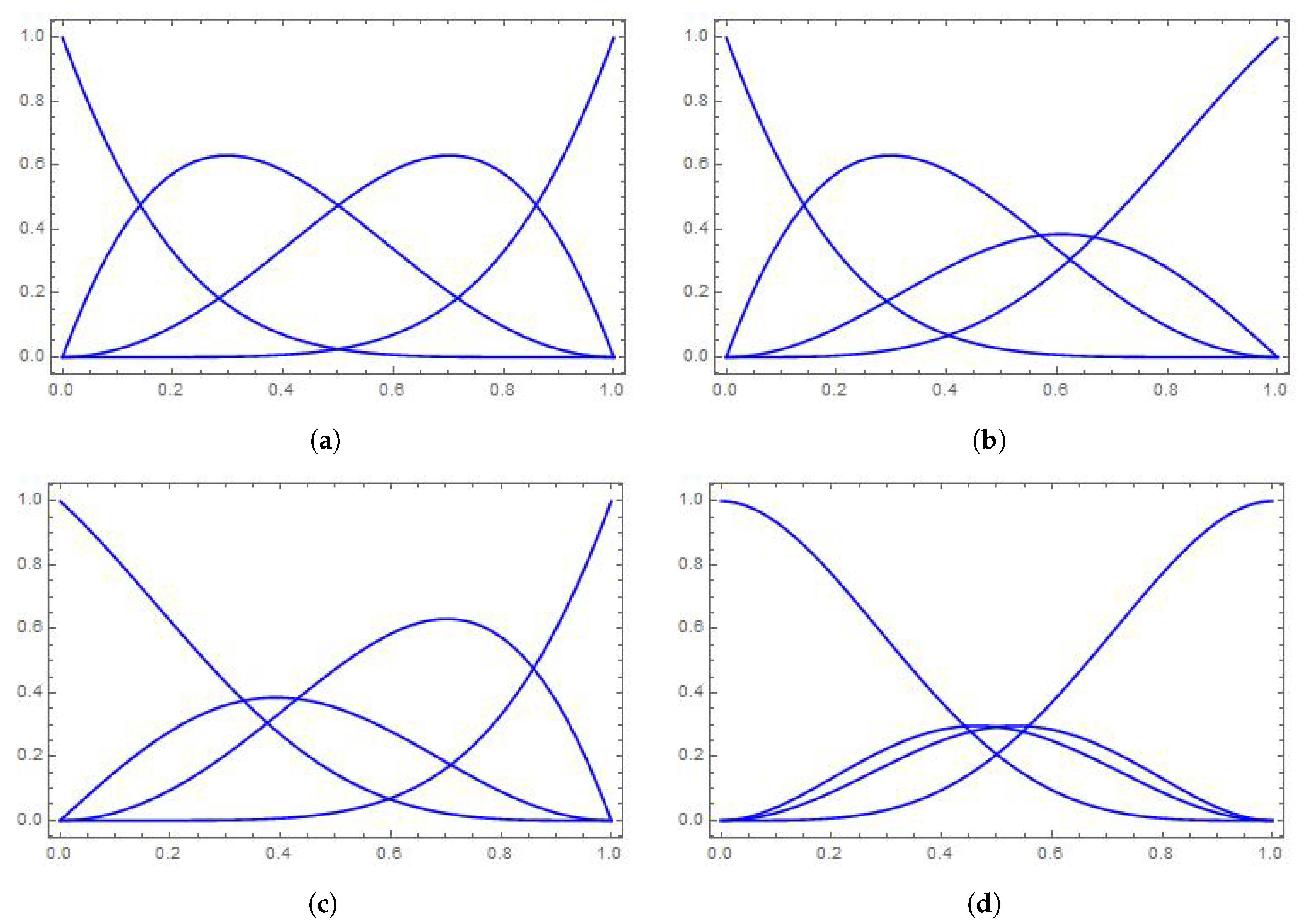
2.1. Cubic Trigonometric Bézier Basis Functions

The definition of a cubic trigonometric Bézier (CT-Bézier) basis function is given as follows [40].

Definition 1.

Let ${\gamma }_1$, ${\gamma }_2$ ∈ $[-2,1]$, for any u ∈ $[0,1]$. The four polynomial functions below

$$\left\{\begin{array}{c}\begin{array}{cc}\hfill w_{0,3}\left(u\right)& ={(1-sin\frac{\pi u}{2})}^2(1-{\gamma }_{1}sin\frac{\pi u}{2}),\hfill \\ \hfill w_{1,3}\left(u\right)& =sin\frac{\pi u}{2}(1-sin\frac{\pi u}{2})(2+{\gamma }_1-{\gamma }_{1}sin\frac{\pi u}{2}),\hfill \\ \hfill w_{2,3}\left(u\right)& =cos\frac{\pi u}{2}(1-cos\frac{\pi u}{2})(2+{\gamma }_2-{\gamma }_{2}cos\frac{\pi u}{2}),\hfill \\ \hfill w_{3,3}\left(u\right)& ={(1-cos\frac{\pi u}{2})}^2(1-{\gamma }_{2}cos\frac{\pi u}{2}),\hfill \end{array}\end{array}\right.$$

(1)

are called CT-Bézier basis functions with the shape parameters ${\gamma }_1$, ${\gamma }_2$. In the case of ${\gamma }_1={\gamma }_2=0$, the basis functions are quadratic trigonometric (QT) polynomials.

The CT-Bézier basis functions for two randomly chosen real values of shape parameters ${\gamma }_1$ and ${\gamma }_2$ are shown in Figure 1. The proof of Theorem 1 is provided in [40].

Theorem 1.

The CT-Bézier basis functions in (1) have the following properties:

(a) 

Non-negativity: $w_{i,3}\left(u\right)\ge 0,i=0,\dots ,3$.

(b) 

Partition of unity: ${\sum }_{i=0}^3{w}_{i,3}\left(u\right)=1$.

(c) 

Monotonicity: with the given parameter u, $w_{0,3}\left(u\right)$ and $w_{3,3}\left(u\right)$ are monotonically decreasing while $w_{1,3}\left(u\right)$ and $w_{2,3}\left(u\right)$ are monotonically increasing for the shape parameters ${\gamma }_1$ and ${\gamma }_2$, respectively.

(d) 

Symmetry: $w_{i,3}(u,{\gamma }_1,{\gamma }_2)=w_{3-i,3}(1-u,{\gamma }_1,{\gamma }_2)$ for $i=0,\dots ,3$.

2.2. Construction of CT-Bézier Curve

Definition 2.

Given control points $b_i(i=0,\dots ,3)$ in ${\mathbb{R}}^2$ or ${\mathbb{R}}^3$, the curve

$$B(u;{\gamma }_1,{\gamma }_2)=\sum _{i=0}^3{w}_{i,3}\left(u\right)b_i,u\in [0,1],$$

(2)

is called the CT-Bézier curve with shape parameters, where ${\gamma }_1,{\gamma }_2\in [-2,1]$ and $w_{i,3}\left(u\right)$ are the basis functions defined in Equation (1).

By using the interpretation of the basic functions, the CT-Bézier curves have the following properties.

(a)

Boundary properties:

$B(0;{\gamma }_1,{\gamma }_2)=b_0$,

$B(1;{\gamma }_1,{\gamma }_2)=b_3$,

$B^{\prime }(0;{\gamma }_1,{\gamma }_2)=\frac{\pi }{2}(2+{\gamma }_1)(b_1-b_0)$,

$B^{\prime }(1;{\gamma }_1,{\gamma }_2)=\frac{\pi }{2}(2+{\gamma }_2)(b_3-b_2)$,

$B^{″}(0;{\gamma }_1,{\gamma }_2)=\frac{{\pi }^2}{2}\left((1+2{\gamma }_1)b_0-(2+2{\gamma }_1)b_1+b_2\right)$,

$B^{″}(1;{\gamma }_1,{\gamma }_2)=\frac{{\pi }^2}{2}\left((1+2{\gamma }_2)b_3-(2+2{\gamma }_2)b_2+b_1\right).$

(b)

Symmetry: $b_0,b_1,b_2,b_3$ and $b_3,b_2,b_1,b_0$ define the same CT-Bézier curve in different parameterizations, i.e.,

$B(u;{\gamma }_1,{\gamma }_2;b_0,b_1,b_2,b_3)$ = $B(1-u;{\gamma }_1,{\gamma }_2;b_3,b_2,b_1,b_0)$, $u\in [0,1]$, ${\gamma }_1,{\gamma }_2\in [-2,1]$.

(c)

Geometric invariance: The CT-Bézier curve has a shape that is independent of the selection of the coordination, i.e., Equation (2) satisfies the following two equations:

$B(u;{\gamma }_1,{\gamma }_2;b_0+q,b_1+q,b_2+q,b_3+q)$ = $B(u;{\gamma }_1,{\gamma }_2;b_0,b_1,b_2,b_3)+q$,

$B(u;{\gamma }_1,{\gamma }_2;b_0\ast T,b_1\ast T,b_2\ast T,b_3\ast T)$ = $B(u;{\gamma }_1,{\gamma }_2;b_0,b_1,b_2,b_3)\ast T$.

where q is an arbitrary vector in ${\mathbb{R}}^2$ or ${\mathbb{R}}^3$ and T is an arbitrary $d\times d$ matrix, $d=2$ or 3.

(d)

Convex hull property: The entire segment of the CT-Bézier curve must lie inside the control polygon.

3. Construction of GDCT-Bézier Surfaces

3.1. Dual Generation of Single-Parameter Family of Planes

Duality is a concept adapted from projective geometry. This concept is useful to construct developable surfaces. As per the duality theory among points and planes, the single parameter family of control points of a curve is dual to a single parameter family of planes. The single parameter family of planes $\left\{{\prod }_u\right\}$ can easily be reached if the control points $R_i$ in a CT-Bézier curve are treated as a control plane. Thus by Equation (2), the single parameter family of plane $\left\{{\prod }_u\right\}$ can be defined as

$$\left\{{\prod }_u\right\}:S(u;{\gamma }_1,{\gamma }_2)=\sum _{i=0}^3{w}_{i,3}\left(u\right)R_i,$$

(3)

where $R_i(i=0,\dots ,3)$ are control points of $\left\{{\prod }_u\right\}$, u is the family of parameter, and ${\gamma }_1,{\gamma }_2$ are shape control parameters of $\left\{{\prod }_u\right\}$. In a three-dimensional projective space, if the coordinates of the control plane are $R_i=(a_i,b_i,c_i,d_i)$ with $i=0,\dots ,3,$ the Equation (3) can be written as

$$\begin{array}{cc}\hfill S(u;{\gamma }_1,{\gamma }_2)& =\sum _{i=0}^3{w}_{i,3}\left(u\right)R_i,\hfill \\ \hfill & =\sum _{i=0}^3{w}_{i,3}\left(u\right)(a_i,b_i,c_i,d_i),\hfill \\ \hfill & =\{g_0\left(u\right),g_1\left(u\right),g_2\left(u\right),g_3\left(u\right)\},\hfill \end{array}$$

(4)

where,

$$\left\{\begin{array}{c}{g}_0\left(u\right)=\sum _{i=0}^3{w}_{i,3}\left(u\right)a_i,\\ g_1\left(u\right)=\sum _{i=0}^3{w}_{i,3}\left(u\right)b_i,\\ g_2\left(u\right)=\sum _{i=0}^3{w}_{i,3}\left(u\right)c_i,\\ g_3\left(u\right)=\sum _{i=0}^3{w}_{i,3}\left(u\right)d_i.\end{array}\right.$$

(5)

3.2. Generalized Enveloping Developable CT-Bézier Surface

Based on the properties and definition of a developable surface, it is comprehended that the envelope of a single-parameter family of planes is a developable surface. The plane corresponding to every value of u in Equation (2) can be defined as

$$g_0\left(u\right)x+g_1\left(u\right)y+g_2\left(u\right)z=g_3\left(u\right).$$

(6)

Equation (6) when differentiated will yield,

$$g_0{}^{\prime }\left(u\right)x+g_1{}^{\prime }\left(u\right)y+g_2{}^{\prime }\left(u\right)z=g_3{}^{\prime }\left(u\right).$$

(7)

According to the third definition from [41], the intersecting line between plane Equations (6) and (7) is the generator of a developable surface, which is symbolized by $L(u;{\gamma }_1,{\gamma }_2)$ and can be computed in terms of its Plücker coordinates $L(u;{\gamma }_1,{\gamma }_2)=(f\left(u\right),h\left(u\right))$ where

$$\begin{array}{cc}\hfill f\left(u\right)& = \left(g_0\left(u\right),g_1\left(u\right),g_2\left(u\right)\right) \times \left(g_0{}^{\prime }\left(u\right),g_1{}^{\prime }\left(u\right),g_2{}^{\prime }\left(u\right)\right),\hfill \\ \hfill & = \left(g_1\left(u\right)g_2{}^{\prime }\left(u\right)-g_2\left(u\right)g_1{}^{\prime }\left(u\right),g_0{}^{\prime }\left(u\right)g_2\left(u\right)-g_0\left(u\right)g_2{}^{\prime }\left(u\right),g_0\left(u\right)g_1{}^{\prime }\left(u\right)-g_1\left(u\right)g_0{}^{\prime }\left(u\right)\right),\hfill \end{array}$$

(8)

and

$$\begin{array}{cc}\hfill h\left(u\right)& = g_3{}^{\prime }\left(u\right)\left(g_0\left(u\right),g_1\left(u\right),g_2\left(u\right)\right) - g_3\left(u\right)\left(g_0{}^{\prime }\left(u\right),g_1{}^{\prime }\left(u\right),g_2{}^{\prime }\left(u\right)\right),\hfill \\ \hfill & = (g_0\left(u\right)g_3{}^{\prime }\left(u\right)-g_3\left(u\right)g_0{}^{\prime }\left(u\right),g_1\left(u\right)g_3{}^{\prime }\left(u\right)-g_3\left(u\right)g_1{}^{\prime }\left(u\right),g_2\left(u\right)g_3{}^{\prime }\left(u\right) - g_3\left(u\right)g_2{}^{\prime }\left(u\right)).\hfill \end{array}$$

(9)

Assume $\varphi \left(u\right)$ to be the nearest point to the origin that lies on the two planes, so it satisfies

$$\left\{\begin{array}{c}\begin{array}{c}\hfill g_0\left(u\right)x+g_1\left(u\right)y+g_2\left(u\right)z=g_3\left(u\right),\\ \hfill g_0{}^{\prime }\left(u\right)x+g_1{}^{\prime }\left(u\right)y+g_2{}^{\prime }\left(u\right)z=g_3{}^{\prime }\left(u\right),\\ \hfill (g_1\left(u\right)g_2{}^{\prime }\left(u\right)-g_2\left(u\right)g_1{}^{\prime }\left(u\right))x+(g_0{}^{\prime }\left(u\right)g_2\left(u\right)-g_0\left(u\right)g_2{}^{\prime }\left(u\right))y& +\hfill \\ \hfill (g_0\left(u\right)g_1{}^{\prime }\left(u\right)-g_1\left(u\right)g_0{}^{\prime }\left(u\right))z=0.\end{array}\end{array}\right.$$

By solving this system of equations, we get

$$\begin{array}{cc}\hfill \varphi \left(u\right)& =\frac{f\times h}{f·f},\hfill \\ \hfill & =\{[g_2\left(u\right)g_0{}^{\prime }\left(u\right)-g_0\left(u\right)g_2{}^{\prime }\left(u\right)][g_2\left(u\right)g_3{}^{\prime }\left(u\right)-g_3\left(u\right)g_2{}^{\prime }\left(u\right)]-[g_0\left(u\right)g_1{}^{\prime }\left(u\right)-g_1\left(u\right)g_0{}^{\prime }\left(u\right)]\hfill \\ \hfill & [g_1\left(u\right)g_3{}^{\prime }\left(u\right)-g_3\left(u\right)g_1{}^{\prime }\left(u\right)],[g_0\left(u\right)g_1{}^{\prime }\left(u\right)-g_1\left(u\right)g_0{}^{\prime }\left(u\right)][g_0\left(u\right)g_3{}^{\prime }\left(u\right)-g_3\left(u\right)g_0{}^{\prime }\left(u\right)]-\hfill \\ & [g_1\left(u\right)g_2{}^{\prime }\left(u\right)-g_2\left(u\right)g_1{}^{\prime }\left(u\right)][g_2\left(u\right)g_3{}^{\prime }\left(u\right)-g_3\left(u\right)g_2{}^{\prime }\left(u\right)],[g_1\left(u\right)g_2{}^{\prime }\left(u\right)-g_2\left(u\right)g_1{}^{\prime }\left(u\right)]\hfill \\ \hfill & [g_1\left(u\right)g_3{}^{\prime }\left(u\right)-g_3\left(u\right)g_1{}^{\prime }\left(u\right)]-[g_2\left(u\right)g_0{}^{\prime }\left(u\right)-g_0\left(u\right)g_2{}^{\prime }\left(u\right)][g_0\left(u\right)g_3{}^{\prime }\left(u\right)-g_3\left(u\right)g_0{}^{\prime }\left(u\right)]\}\hfill \\ \hfill & /\{{[g_1\left(u\right)g_2{}^{\prime }\left(u\right)-g_2\left(u\right)g_1{}^{\prime }\left(u\right)]}^2+{[g_2\left(u\right)g_0{}^{\prime }\left(u\right)-g_0\left(u\right)g_2{}^{\prime }\left(u\right)]}^2+{[g_0\left(u\right)g_1{}^{\prime }\left(u\right)-g_1\left(u\right)g_0{}^{\prime }\left(u\right)]}^2\}.\hfill \end{array}$$

Therefore, the line $L(u;{\gamma }_1,{\gamma }_2)$ can be represented as

$$T(k,u;{\gamma }_1,{\gamma }_2)=kf\left(u\right)+\varphi \left(u\right),k\in (-\infty ,\infty ),$$

(10)

when the parameter u family range is $[0,1]$ and the line $L(u;{\gamma }_1,{\gamma }_2)$ produces a developable surface with shape parameter ${\gamma }_1,{\gamma }_2$. It is apparent from the above calculation process that a developable surface can be created when the control planes are provided.

3.3. Generalized Spine Curve Developable CT-Bézier surface

This section includes one more approach in constructing developable surfaces. With regard to Definition 3 in [41], the three successive planes in the family of a plane $\left\{{\prod }_u\right\}$ intersect at a characteristic point and can be achieved by intersecting Equations (6) and (7), and the second derivative of Equation (6) produces the third plane.

$${g_0}^{″}\left(u\right)x+g_1{}^{″}\left(u\right)y+g_2{}^{″}\left(u\right)z=g_3{}^{″}\left(u\right).$$

(11)

Significantly, the characteristic argument can be reached by solving the following set of equations:

$$\left\{\begin{array}{c}{g}_0\left(u\right)x+g_1\left(u\right)y+g_2\left(u\right)z=g_3\left(u\right),\\ g_0{}^{\prime }\left(u\right)x+g_1{}^{\prime }\left(u\right)y+g_2{}^{\prime }\left(u\right)z=g_3{}^{\prime }\left(u\right),\\ g_0{}^{″}\left(u\right)x+g_1{}^{″}\left(u\right)y+g_2{}^{″}\left(u\right)z=g_3{}^{″}\left(u\right).\end{array}\right.$$

(12)

Hence, the coordinate of the characteristic point $\rho \left(u\right)$ is given by

$$x=\frac{\left[\begin{array}{ccc}{g}_3\left(u\right)& g_1\left(u\right)& g_2\left(u\right)\\ g_3{}^{\prime }\left(u\right)& g_1{}^{\prime }\left(u\right)& g_2{}^{\prime }\left(u\right)\\ g_3{}^{″}\left(u\right)& g_1{}^{″}\left(u\right)& g_2{}^{″}\left(u\right)\end{array}\right]}{\left[\begin{array}{ccc}{g}_0\left(u\right)& g_1\left(u\right)& g_2\left(u\right)\\ g_0{}^{\prime }\left(u\right)& g_1{}^{\prime }\left(u\right)& g_2{}^{\prime }\left(u\right)\\ g_0{}^{″}\left(u\right)& g_1{}^{″}\left(u\right)& g_2{}^{″}\left(u\right)\end{array}\right]},y=\frac{\left[\begin{array}{ccc}{g}_0\left(u\right)& g_3\left(u\right)& g_2\left(u\right)\\ g_0{}^{\prime }\left(u\right)& g_3{}^{\prime }\left(u\right)& g_2{}^{\prime }\left(u\right)\\ g_0{}^{″}\left(u\right)& g_3{}^{″}\left(u\right)& g_2{}^{″}\left(u\right)\end{array}\right]}{\left[\begin{array}{ccc}{g}_0\left(u\right)& g_1\left(u\right)& g_2\left(u\right)\\ g_0{}^{\prime }\left(u\right)& g_1{}^{\prime }\left(u\right)& g_2{}^{\prime }\left(u\right)\\ g_0{}^{″}\left(u\right)& g_1{}^{″}\left(u\right)& g_2{}^{″}\left(u\right)\end{array}\right]},z=\frac{\left[\begin{array}{ccc}{g}_0\left(u\right)& g_1\left(u\right)& g_3\left(u\right)\\ g_0{}^{\prime }\left(u\right)& g_1{}^{\prime }\left(u\right)& g_3{}^{\prime }\left(u\right)\\ g_0{}^{″}\left(u\right)& g_1{}^{″}\left(u\right)& g_3{}^{″}\left(u\right)\end{array}\right]}{\left[\begin{array}{ccc}{g}_0\left(u\right)& g_1\left(u\right)& g_2\left(u\right)\\ g_0{}^{\prime }\left(u\right)& g_1{}^{\prime }\left(u\right)& g_2{}^{\prime }\left(u\right)\\ g_0{}^{″}\left(u\right)& g_1{}^{″}\left(u\right)& g_2{}^{″}\left(u\right)\end{array}\right]}.$$

When parameter u varies in the range $[0,1]$, $\rho \left(u\right)$ can generate a spine curve which can be represented in parametric form such as below:

$$T(m,u;{\gamma }_1,{\gamma }_2)=\rho \left(u\right)+m\rho {}^{\prime }\left(u\right),u\in [0,1],m\in (-\infty ,\infty ).$$

(13)

3.4. Developable Surface Interpolating Geodesic CT-Bézier Curve with Parameters

A geodesic is the shortest possible line between two points on a sphere or other curved surface. This section involves the construction of developable surface through a given cubic trigonometric Bézier curve, where the curve is the geodesic of the surface.

Theorem 2.

A curve is a geodesic on the surface $T(m,u)$ only when the principal normal $\zeta \left(u\right)$ is $\left|\right|$ to the normal $N(m_0,u)$ at every point on the curve.

Proof. 

Suppose that $c\left(u\right)$ is a curve on the surface $T(m,u)$ and $\varphi$ is an arbitrary point on the curve $c\left(u\right)$, $N(m_0,u)$ is the normal vector at point $\varphi$, $\zeta \left(u\right)$ is the principal normal, $\theta$ is the angle between $\zeta \left(u\right)$ and $N(m_0,u)$ and $k_g$ is the geodesic curvature. Then, according to the definitions of geodesic curve and $k_g$

$$k_g=\pm ksin\theta =0.$$

Since $k\ne 0$, the $\theta =0$ or $\theta =\pi$ then $\zeta \left(u\right)$ is $\left|\right|$$N(m_0,u)$. This proves the theorem. □

Theorem 3.

When a CT-Bézier curve with shape parameters ${\gamma }_1,{\gamma }_2$ is given, a developable surface that is geodesic to the developable surface must exist through it.

Proof. 

Given a CT-Bézier curve $c(u;{\gamma }_1,{\gamma }_2)$, we have the respective ruled surface

$$T(m,u;{\gamma }_1,{\gamma }_2)=c(u;{\gamma }_1,{\gamma }_2)+m{c}_1(u;{\gamma }_1,{\gamma }_2),u\in [0,1],m\in (-\infty ,+\infty ).$$

When a curve $c(u;{\gamma }_1,{\gamma }_2)$ is geodesic to Theorem 2, we have

$$T(0,u;{\gamma }_1,{\gamma }_2)=c(u;{\gamma }_1,{\gamma }_2),\zeta (u;{\gamma }_1,{\gamma }_2)\left|\right|N(0,u;{\gamma }_1,{\gamma }_2),$$

where $\zeta (u;{\gamma }_1,{\gamma }_2)$ and $N(0,u;{\gamma }_1,{\gamma }_2)$ are the principal normal and normal vector of the curve. For simplicity we omit the variable and parameters.

$$N(0,u;{\gamma }_1,{\gamma }_2)=T_u\times T_m=(c{}^{\prime }+m{c}_1{}^{\prime })\times c_1{|}_{m=0}=c{}^{\prime }\times c_1{}^{\prime }$$

and

$$\zeta (u;{\gamma }_1,{\gamma }_2)=\frac{(c{}^{\prime }·c{}^{\prime })·c{}^{″}-(c{}^{\prime }·c″)·c{}^{\prime }}{|c{}^{\prime }\left|\right|c{}^{\prime }\times c{}^{″}|}.$$

Because $\zeta (u;{\gamma }_1,{\gamma }_2)$ is parallel to $N(0,u;{\gamma }_1,{\gamma }_2)$ and $c{}^{\prime }$ is perpendicular to N, the vector $c_1$ must be in the plane spanned by $c{}^{\prime }$ and $c{}^{\prime }$×$c{}^{″}$. Let

$$c_1={\mu }_{1}c{}^{\prime }+{\mu }_2(c{}^{\prime }\times c{}^{″}).$$

According to the developable conditions, we have

$$\begin{array}{c}\begin{array}{ccc}\hfill & \hfill & \hfill (c{}^{\prime },{\mu }_{1}c{}^{\prime }+{\mu }_2(c{}^{\prime }\times c{}^{″}),({\mu }_{1}c{}^{\prime }+{\mu }_2(c{}^{\prime }\times c{}^{″})){}^{\prime })=0\\ \hfill \iff & \hfill & \hfill (c{}^{\prime },{\mu }_{1}c{}^{\prime }+{\mu }_2(c{}^{\prime }\times c{}^{″}),{\mu }_1{}^{\prime }c{}^{\prime }+{\mu }_{1}c{}^{″}+{\mu }_2{}^{\prime }c{}^{\prime }\times c{}^{″}+{\mu }_{2}c{}^{\prime }\times c^{‴}=0\\ \hfill \iff & \hfill & \hfill (c{}^{\prime },{\mu }_2(c{}^{\prime }\times c{}^{″}),{\mu }_{1}c{}^{″}+{\mu }_2{}^{\prime }c{}^{\prime }\times c{}^{″}+{\mu }_{2}c{}^{\prime }\times c^{‴})=0\\ \hfill \stackrel{{\mu }_2\ne 0}{\iff }& \hfill & \hfill [(c{}^{\prime }\times c{}^{″})\times c{}^{\prime }]·({\mu }_{1}c{}^{″}+{\mu }_{2}c{}^{\prime }\times c^{‴})=0\\ \hfill \iff & \hfill & \hfill [(c{}^{\prime }·c{}^{\prime })c{}^{″}-(c{}^{″}·c{}^{\prime })c{}^{\prime }]·({\mu }_{1}c{}^{″}+{\mu }_{2}c{}^{\prime }\times c^{‴})=0\\ \hfill \iff & \hfill & \hfill \left(\right|c{}^{\prime }{|}^2|c{}^{″}{|}^2-|c{}^{\prime }·c{}^{″}{|}^2){\mu }_1={\left|c{}^{\prime }\right|}^2(c{}^{\prime },c{}^{″},c^{‴}){\mu }_2.\end{array}\end{array}$$

(14)

that is,

$$\begin{array}{c}\hfill T(m,u;{\gamma }_1,{\gamma }_2)=c(u;{\gamma }_1,{\gamma }_2)+m({\mu }_{1}c{}^{\prime }(u;{\gamma }_1,{\gamma }_2)+{\mu }_2(c{}^{\prime }(u;{\gamma }_1,{\gamma }_2)\times c{}^{″}(u;{\gamma }_1,{\gamma }_2))),\\ \hfill u\in [0,1],m\in (-\infty ,+\infty ).\end{array}$$

(15)

Which interpolate the given curve $c\left(u\right)$ and $c\left(u\right)$ is a geodesic of the developable surface, where ${\mu }_1$ and ${\mu }_2$ satisfy the Equation (14). □

In a special case, if we choose $l2\left(t\right)=1$.

3.5. Analysis Properties of the GDCT-Bézier Surface

According to the single parameter family of planes $\left\{{\prod }_u\right\}$, the 1st and 2nd derivatives of Equation (3) are

$$\left\{\begin{array}{c}S{}^{\prime }(u;{\gamma }_1,{\gamma }_2)=R_0{w}_{0,3}{}^{\prime }\left(u\right)+R_1{w}_{1,3}{}^{\prime }\left(u\right)+R_2{w}_{2,3}{}^{\prime }\left(u\right)+R_3{w}_{3,3}{}^{\prime }\left(u\right),\\ S{}^{″}(u;{\gamma }_1,{\gamma }_2)=R_0{w}_{0,3}{}^{″}\left(u\right)+R_1{w}_{1,3}{}^{″}\left(u\right)+R_2{w}_{2,3}{}^{″}\left(u\right)+R_3{w}_{3,3}{}^{″}\left(u\right).\end{array}\right.$$

(16)

Therefore, the planes corresponding to $u=0$ and $u=1$ in $\left\{{\prod }_u\right\}$ have the following characteristics:

$$\left\{\begin{array}{c}\begin{array}{cc}\hfill S(0;{\gamma }_1,{\gamma }_2)& =R_0,\hfill \\ \hfill S{}^{\prime }(0;{\gamma }_1,{\gamma }_2)& =\frac{\pi }{2}(2+{\gamma }_1)(R_1-R_0),\hfill \\ \hfill S{}^{″}(0;{\gamma }_1,{\gamma }_2)& =\frac{{\pi }^2}{2}\left((1+2{\gamma }_1)R_0-(2+2{\gamma }_1)R_1+R_2\right),\hfill \end{array}\end{array}\right.$$

(17)

and

$$\left\{\begin{array}{cc}\hfill S(1;{\gamma }_1,{\gamma }_2)& =R_3,\hfill \\ \hfill S{}^{\prime }(1;{\gamma }_1,{\gamma }_2)& =\frac{\pi }{2}(2+{\gamma }_2)(R_3-R_2),\hfill \\ \hfill S{}^{″}(1;{\gamma }_1,{\gamma }_2)& =\frac{{\pi }^2}{2}\left((1+2{\gamma }_2)R_3-(2+2{\gamma }_2)R_2+R_1\right).\hfill \end{array}\right.$$

(18)

The first Equations of (17) and (18) shows that the first and last planes corresponding to $u=0$ and $u=1$ in $\left\{{\prod }_u\right\}$ are given by the designer as the first and last control planes and they are both tangential to the GDCT-Bézier surface along its generator, at $u=0$ and $u=1$. In addition, the generator of the GDCT-Bézier surface at $u=0$ is the intersection between two planes, represented by the first two Equations of (17), called the starting generator. Therefore, the generator $L(0;{\gamma }_1,{\gamma }_2)$ is the intersection of two planes $R_0$ and $\frac{\pi }{2}(2+{\gamma }_1)(R_1-R_0)$ and can be written as

$$\left\{\begin{array}{c}\begin{array}{cc}\hfill r_0·X& =d_0,\hfill \\ \hfill \frac{\pi }{2}(2+{\gamma }_1)(r_1-r_0)·X& =\frac{\pi }{2}(2+{\gamma }_1)(d_1-d_0),\hfill \end{array}\end{array}\right.$$

(19)

where $r_0=(a_0,b_0,c_0)$, $r_1=(a_1,b_1,c_1)$, and $X=(x,y,z)$.

$R_1$ can be accomplished by the linear combination of two planes in Equation (19) and the generator $L(0;{\gamma }_1,{\gamma }_2)$ is the intersection of $R_0$ and $R_1$. Furthermore, the generator $L(0;{\gamma }_1,{\gamma }_2)$ dual to the line that connects the points $R_0$ and $R_1$, which is tangential to GDCT-Bézier curve defined by $R_0,R_1,R_2,R_3$. Similarly, the ending generator $L_{1;{\gamma }_1,{\gamma }_2}$ corresponding to $u=1$ is the intersection of $R_2$ and $R_3$ in Equation (18).

In addition, the Equations (17) and (18) can be written in matrix form as:

$$\left[\begin{array}{c}{R}_0\\ R_1\\ R_2\end{array}\right]=\left[\begin{array}{ccc}1& 0& 0\\ 1& \frac{1}{\frac{\pi }{2}(2+{\gamma }_1)}& 0\\ 1& \frac{{\pi }^2(1+{\gamma }_1)}{\frac{{\pi }^3}{4}(2+{\gamma }_1)}& \frac{1}{\frac{{\pi }^2}{2}}\end{array}\right]\left[\begin{array}{c}S(0;{\gamma }_1,{\gamma }_2)\\ S{}^{\prime }(0;{\gamma }_1,{\gamma }_2)\\ S{}^{″}(0;{\gamma }_1,{\gamma }_2)\end{array}\right]$$

(20)

and

$$\left[\begin{array}{c}{R}_3\\ R_2\\ R_1\end{array}\right]=\left[\begin{array}{ccc}1& -\frac{{\pi }^2(1+{\gamma }_2)}{\frac{{\pi }^3}{4}(2+{\gamma }_2)}& \frac{1}{\frac{{\pi }^2}{2}}\\ 1& -\frac{1}{\frac{\pi }{2}(2+{\gamma }_1)}& 0\\ 1& 0& 0\end{array}\right]\left[\begin{array}{c}S(1;{\gamma }_1,{\gamma }_2)\\ S{}^{\prime }(1;{\gamma }_1,{\gamma }_2)\\ S{}^{″}(1;{\gamma }_1,{\gamma }_2)\end{array}\right]$$

(21)

Since the intersection of the $S,S{}^{\prime },S{}^{″}$ planes is the spine curve of the GDCT-Bézier surface, the characteristic point and plane coordinates of $R_0,R_1,R_2$ will be achieved through the linear combination of $S,S{}^{\prime },S{}^{″}$ according to Equation (20). So, the intersection of plane coordinates $R_0,R_1,R_2$ is the spine curve GDCT-Bézier surface characteristic point on $T(m,0;{\gamma }_1,{\gamma }_2)$. Similarly, in Equation (21), the control points $R_1,R_2,R_3$ define the characteristic point on $T(m,1;{\gamma }_1,{\gamma }_2)$.

4. Continuity Conditions between GDCT-Bézier Surfaces

Many complex engineering surfaces are built in on CAD/CAM systems, but the construction of a complex surface with a single surface is highly challenging. Therefore, the promising features seem very important to ensure a smooth relationship between the adjacent GDCT-Bézier surfaces [13,42]. However, the $G^1$, Farin–Boehm $G^2$, and $G^2$ Beta continuity are currently the standards for continuity measurement between two adjacent developable surfaces [17,43,44].

Assuming two GDCT-Bézier surfaces must be spliced together, this is represented by the expression

$$\left\{\begin{array}{c}\left\{{\prod }_{u,1}\right\}:S_1(u;{\gamma }_{1,1},{\gamma }_{2,1})=\{g_{0,1}\left(u\right),g_{1,1}\left(u\right),g_{2,1}\left(u\right),g_{3,1}\left(u\right)\},\hspace{1em}\hspace{1em}0\le u\le 1,\\ \left\{{\prod }_{u,2}\right\}:S_2(u;{\gamma }_{1,2},{\gamma }_{2,2})=\{g_{0,2}\left(u\right),g_{1,2}\left(u\right),g_{2,2}\left(u\right),g_{3,2}\left(u\right)\},\hspace{1em}\hspace{1em}0\le u\le 1.\end{array}\right.$$

(22)

where ${\gamma }_{1,i},{\gamma }_{2,i}(i=1,2)$ are shape parameters and $R_{i,1},R_{i,2}(i=0,1,2,3)$ are control planes.

4.1. The $G^1$ Continuity Conditions of GDCT-Bézier Surfaces

In accordance with the description and analysis for $G^1$ smooth continuity between two parametrical curves in [43], the $G^1$ continuity conditions in Equation (22) can be computed as follows.

Theorem 4.

The necessary and sufficient conditions for $G^1$ smooth continuity between two adjacent GDCT-Bézier surfaces in Equation (22) at the joint are

$$\left\{\begin{array}{c}\begin{array}{cc}\hfill R_{0,2}& =R_{3,1},\hfill \\ \hfill R_{1,2}& =\left(1+\frac{(2+{\gamma }_{2,1})}{\phi (2+{\gamma }_{1,2}}\right)R_{3,1}-\frac{(2+{\gamma }_{2,1})}{\phi (2+{\gamma }_{1,2})}{R}_{2,1},\hfill \end{array}\end{array}\right.$$

(23)

where $\phi >0$ is a constant.

Proof. 

To ensure $G^1$ continuity at the joint, the two developable surfaces must fulfill the following conditions:

$$\left\{\begin{array}{c}\begin{array}{cc}\hfill S_1\left(1\right)& =S_2\left(0\right),\hfill \\ \hfill S_1{}^{\prime }\left(1\right)& =\phi S_2{}^{\prime }\left(0\right).\hfill \end{array}\end{array}\right.$$

(24)

Based on Equations (17) and (18), $S_1\left(1\right)$ and $S_2\left(0\right)$ can be given by

$$\left\{\begin{array}{c}{S}_1(1;{\gamma }_{1,1},{\gamma }_{2,1})=R_{3,1},\\ S_2(0;{\gamma }_{1,2},{\gamma }_{2,2})=R_{0,2}.\end{array}\right.$$

Substituting the values of $S_1(1;{\gamma }_{1,1},{\gamma }_{2,1})$ and $S_2(0;{\gamma }_{1,2},{\gamma }_{2,2})$ into Equation (24), we get

$$R_{0,2}=R_{3,1}.$$

(25)

This implies that for the stability of $G^1$, the two surfaces first require a shared control plane. Next, based on Equations (17) and (18), $S_1{}^{\prime }\left(1\right)$ and $S_2{}^{\prime }\left(0\right)$ can be given by

$$\left\{\begin{array}{c}{S}_1{}^{\prime }(1;{\gamma }_{1,1},{\gamma }_{2,1})=\frac{\pi }{2}(2+{\gamma }_{2,1})(R_{3,1}-R_{2,1}),\\ S_2{}^{\prime }(0;{\gamma }_{1,2},{\gamma }_{2,2})=\frac{\pi }{2}(2+{\gamma }_{1,2})(R_{1,2}-R_{0,2}).\end{array}\right.$$

(26)

Combining Equation (26) according to the second Equation of (24), we get

$$\frac{\pi }{2}(2+{\gamma }_{2,1})(R_{3,1}-R_{2,1})=\phi \frac{\pi }{2}(2+{\gamma }_{1,2})(R_{1,2}-R_{0,2}).$$

(27)

Finally, from Equation (25), the Equation of (27) can be written as

$$R_{1,2}=\left(1+\frac{(2+{\gamma }_{2,1})}{\phi (2+{\gamma }_{1,2})}\right)R_{3,1}-\frac{(2+{\gamma }_{2,1})}{\phi (2+{\gamma }_{1,2})}{R}_{2,1}.$$

(28)

Thus, Equations (25) and (28) are the $G^1$ continuity conditions of the two adjacent GDCT-Bézier surfaces. □

4.2. Farin–Boehm $G^2$ Continuity Conditions of GDCT-Bézier Surfaces

Theorem 5.

The conditions needed and necessary for Farin–Boehm $G^2$ continuity between the two GDCT-Bézier surfaces in Equation (22) are

$$\left\{\begin{array}{c}\begin{array}{cc}\hfill R_{0,2}& =R_{3,1},\hfill \\ \hfill R_{1,2}& =\left(1+\frac{(2+{\gamma }_{2,1})}{(2+{\gamma }_{1,2}}\right)R_{3,1}-\frac{(2+{\gamma }_{2,1})}{(2+{\gamma }_{1,2})}{R}_{2,1},\hfill \\ \hfill R_{2,2}& =2\left(\frac{(1+{\gamma }_{2,1})(2+{\gamma }_{1,2})+(1+{\gamma }_{1,2})(2+{\gamma }_{2,1})}{(2+{\gamma }_{1,2})}\right)(R_{3,1}-R_{2,1})+R_{1,1}.\hfill \end{array}\end{array}\right.$$

(29)

Proof. 

In order to obtain the Farin–Boehm $G^2$ continuity, the two surfaces need to satisfy the following

$$\left\{\begin{array}{cc}\hfill S_2\left(0\right)& =S_1\left(1\right),\hfill \\ \hfill S_2{}^{\prime }\left(0\right)& =S_1{}^{\prime }\left(1\right),\hfill \\ \hfill S_2{}^{″}\left(0\right)& =S_1{}^{″}\left(1\right).\hfill \end{array}\right.$$

(30)

Based on Equations (17) and (18), we have

$$\left\{\begin{array}{c}\begin{array}{cc}\hfill S_2(0;{\gamma }_{1,2},{\gamma }_{2,2})& =R_{0,2},\hfill \\ \hfill S_2{}^{\prime }(0;{\gamma }_{1,2},{\gamma }_{2,2})& =\frac{\pi }{2}(2+{\gamma }_{1,2})(R_{1,2}-R_{0,2}),\hfill \\ \hfill S_2{}^{″}(0;{\gamma }_{1,2},{\gamma }_{2,2})& =\frac{{\pi }^2}{2}\left((1+2{\gamma }_{1,2})R_{0,2}-(2+2{\gamma }_{1,2})R_{1,2}+R_{2,2}\right),\hfill \end{array}\end{array}\right.$$

(31)

and

$$\left\{\begin{array}{cc}\hfill S_1(1;{\gamma }_{1,1},{\gamma }_{2,1})& =R_{3,1},\hfill \\ \hfill S_1{}^{\prime }(1;{\gamma }_{1,1},{\gamma }_{2,1})& =\frac{\pi }{2}(2+{\gamma }_{2,1})(R_{3,1}-R_{2,1}),\hfill \\ \hfill S_1{}^{″}(1;{\gamma }_{1,1},{\gamma }_{2,1})& =\frac{{\pi }^2}{2}\left((1+2{\gamma }_{2,1})R_{3,1}-(2+2{\gamma }_{2,1})R_{2,1}+R_{1,1}\right).\hfill \end{array}\right.$$

(32)

Substitute Equations (31) and (32) into Equation (30), the conclusion in Equation (29) can be obtained. □

4.3. $G^2$ Beta Continuity Conditions of GDCT-Bézier Surfaces

Theorem 6.

The conditions needed and necessary for $G^2$ Beta continuity continuity between the two GDCT-Bézier surfaces in Equation (22) are

$$\left\{\begin{array}{c}\begin{array}{cc}\hfill R_{0,2}& =R_{3,1},\hfill \\ \hfill R_{1,2}& =\left(1+\phi \frac{(2+{\gamma }_{2,1})}{(2+{\gamma }_{1,2}}\right)R_{3,1}-\phi \frac{(2+{\gamma }_{2,1})}{(2+{\gamma }_{1,2})}{R}_{2,1},\hfill \\ \hfill R_{2,2}& =\left(\frac{(2+{\gamma }_{1,2})\left(1+{\phi }^2(1+2{\gamma }_{2,1})+\frac{\psi }{\pi }(2+{\gamma }_{2,1})\right)+2\phi (1+{\gamma }_{1,2})(2+{\gamma }_{2,1})}{(2+{\gamma }_{1,2})}\right)R_{3,1}\hfill \\ \hfill & -\left(\frac{(2+{\gamma }_{1,2})\left(2{\phi }^2(1+{\gamma }_{2,1})+\frac{\psi }{\pi }(2+{\gamma }_{2,1})\right)+2\phi (1+{\gamma }_{1,2})(2+{\gamma }_{2,1})}{(2+{\gamma }_{1,2})}\right)R_{2,1}\hfill \\ \hfill & +{\phi }^2{R}_{1,1}.\hfill \end{array}\end{array}\right.$$

(33)

where $\phi >0$, and ψ is an arbitrary constant.

Proof. 

To reach $G^2$ Beta continuity, the two surfaces need to satisfy

$$\left\{\begin{array}{c}\begin{array}{cc}\hfill S_2\left(0\right)& =S_1\left(1\right),\hfill \\ \hfill S_2{}^{\prime }\left(0\right)& =\phi S_1{}^{\prime }\left(1\right),\hfill \\ \hfill S_2{}^{″}\left(0\right)& ={\phi }^2{S}_1{}^{″}\left(1\right)+\psi S_1{}^{\prime }\left(1\right).\hfill \end{array}\end{array}\right.$$

(34)

Substituting Equations (31) and (32), the derivatives of $S_1(u;{\gamma }_{1,1},{\gamma }_{2,1})$ and $S_2(u;{\gamma }_{1,2},{\gamma }_{2,2})$ at $u=1$ and $u=0$, into Equation (34), then Equation (33) can be obtained. □

5. Design Examples of GDCT-Bézier Surface

In this section, some examples are presented to demonstrate the construction of cubic trigonometric surfaces by means of control planes. Here, the plane coordinates $(a_i,b_i,c_i,d_i)$ of each $R_i(i=0,1,2,3)$ control plane can be defined by its center point $(a_i,b_i,c_i)$ and $d_i=a_i^2+b_i^2+c_i^2$ is the distance. It should be noted that this sort of representation is not valid where the origin is the center point.

Distinctly, the envelop and spine curve family of developable surfaces, as well as piecewise- developable surfaces with some smooth continuity, are being generated by the proposed method used in this paper. The resulting shapes are shown in Figure 2, Figure 3, Figure 4, Figure 5, Figure 6, Figure 7 and Figure 8. These surfaces can be viewed from different angles and the designer can change the shape manually by adjusting their shape parameter values without re-determining the control planes, which solves the problems of the methods in [1,45,46,47,48,49,50]. Moreover, the GDCT-Bézier surfaces reserve many properties of the traditional Bézier surfaces, especially when the shape parameters have values equal to 1.

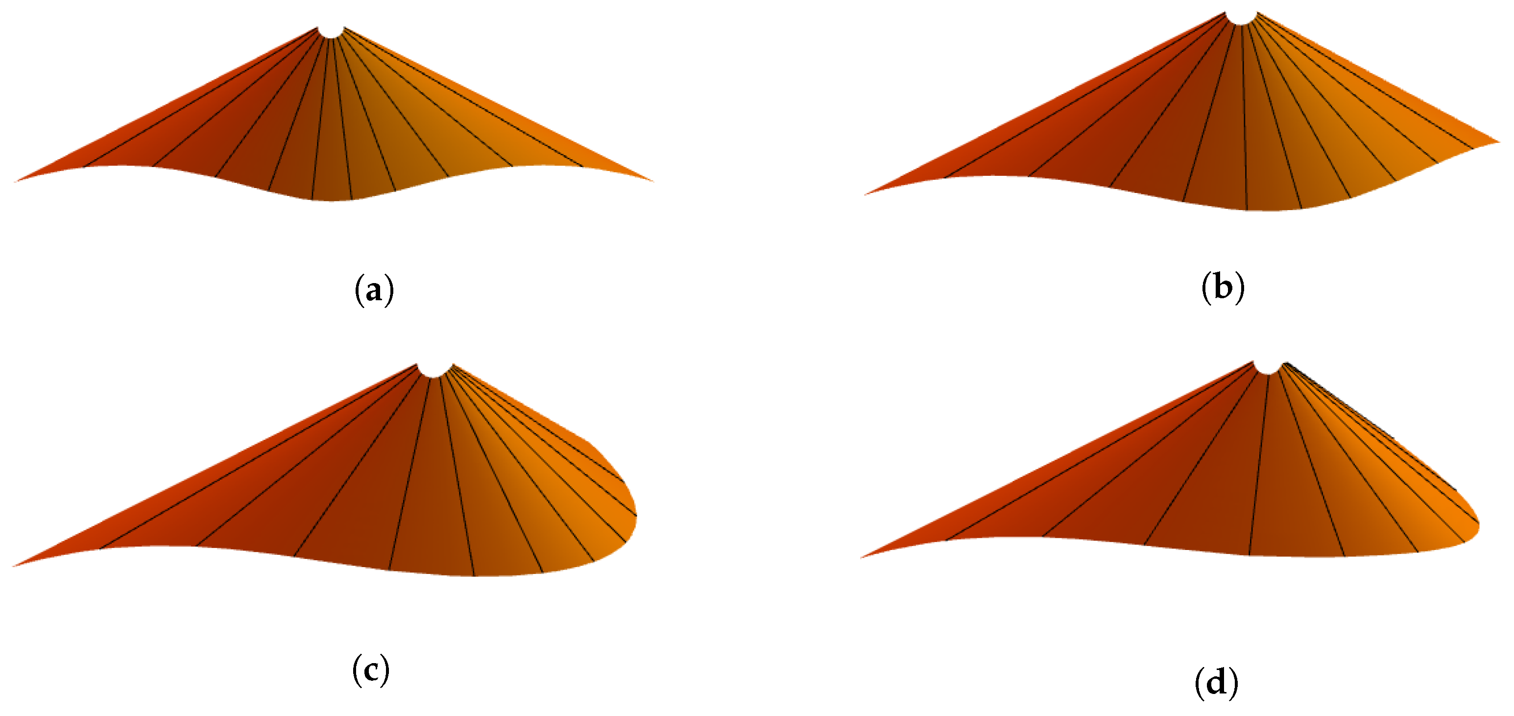
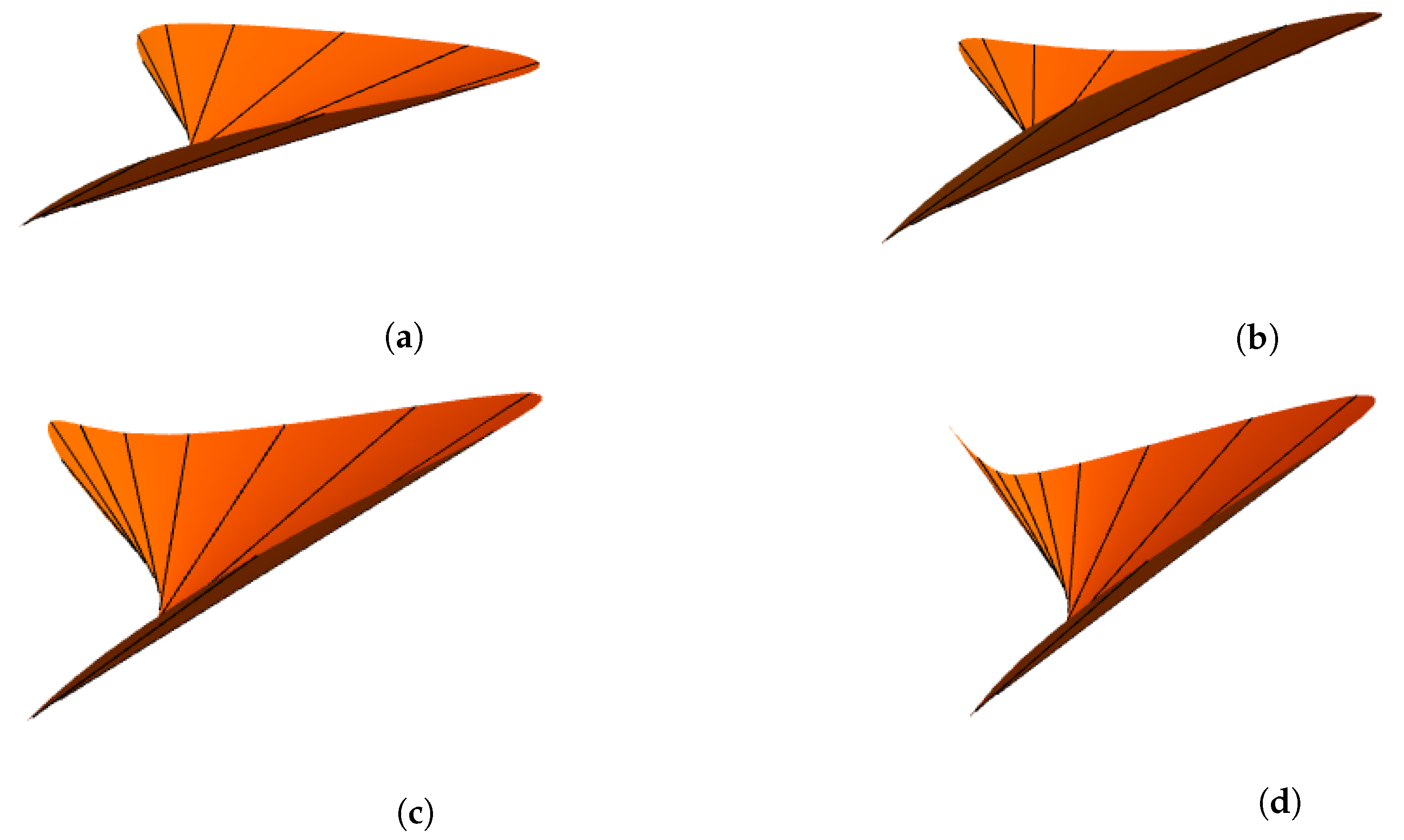
5.1. Examples of Enveloping GDCT-Bézier Surfaces

In this example, the construction of the cubic trigonometric enveloping developable Bézier surface is shown. Assume the coordinates of the control planes are

$$\begin{array}{ll}{R}_0=(5\sqrt{2},-5\sqrt{2},5,125),& R_1=(-5\sqrt{2},-5\sqrt{2},5,125),\\ R_2=(-5\sqrt{2},5\sqrt{2},5,125),& R_3=(5\sqrt{2},5\sqrt{2},5,125).\end{array}$$

Here, we presume that in designing the enveloping developable surfaces, the center points of four control planes are coplanar and each has an equal distance to the origin. When ${\gamma }_1$, ${\gamma }_2$ assumes different values, a family of enveloping GDCT-Bézier surfaces with different shapes can be constructed under the conditions of the specified control planes (see Figure 2 and Figure 3).

• When modifying the value of ${\gamma }_1$ and keeping ${\gamma }_2$ unchanged, the $T(1;{\gamma }_1,{\gamma }_2)$ generator retains the same length and location. However, the length of the generator $T(0;{\gamma }_1,{\gamma }_2)$ becomes longer when we increase the value of ${\gamma }_1$, but its position remains unchanged.
• If the value of shape parameter ${\gamma }_1$ is constant and ${\gamma }_2$ is adjusted, the generator $T(0;{\gamma }_1,{\gamma }_2)$ retains the same length and position. However, the position of generator $T(1;{\gamma }_1,{\gamma }_2)$ also remains unchanged, but its length increases when we increase the value of ${\gamma }_2$.

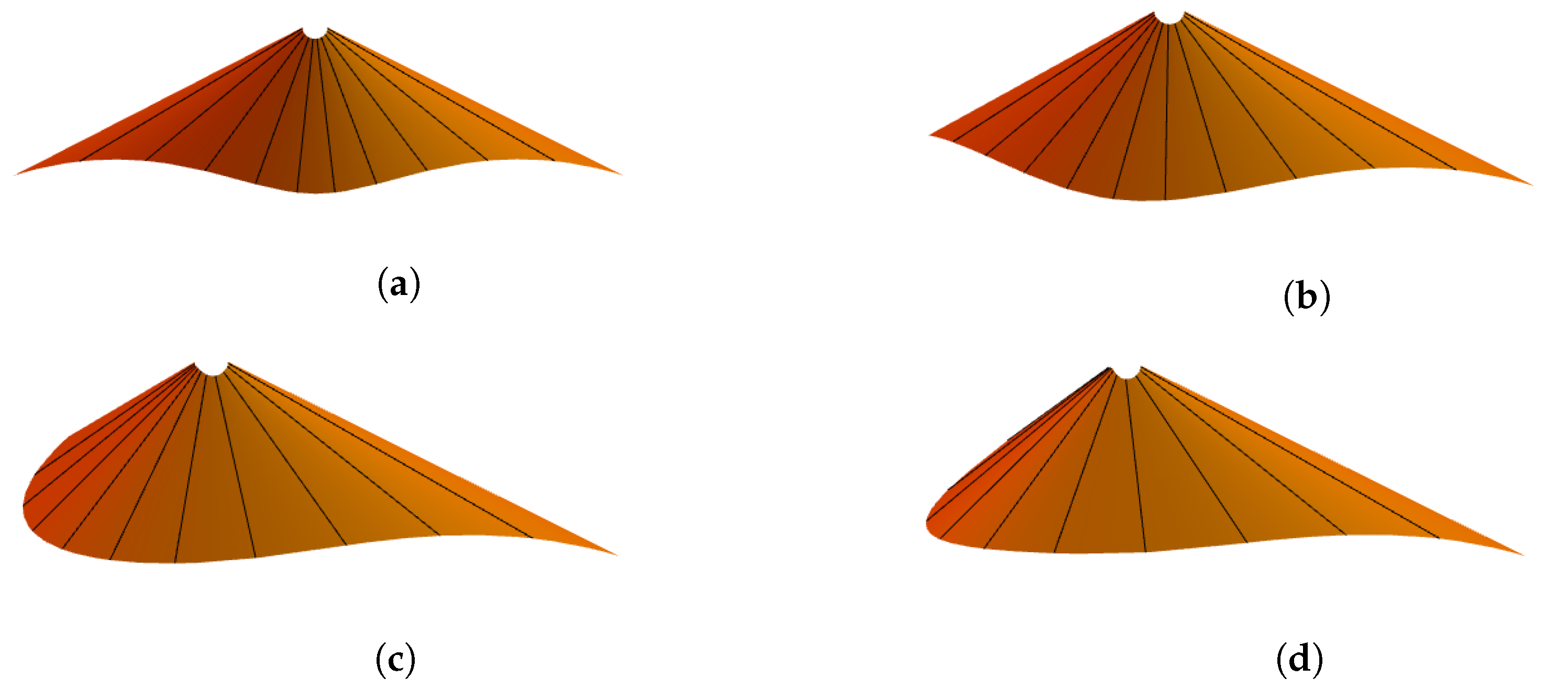
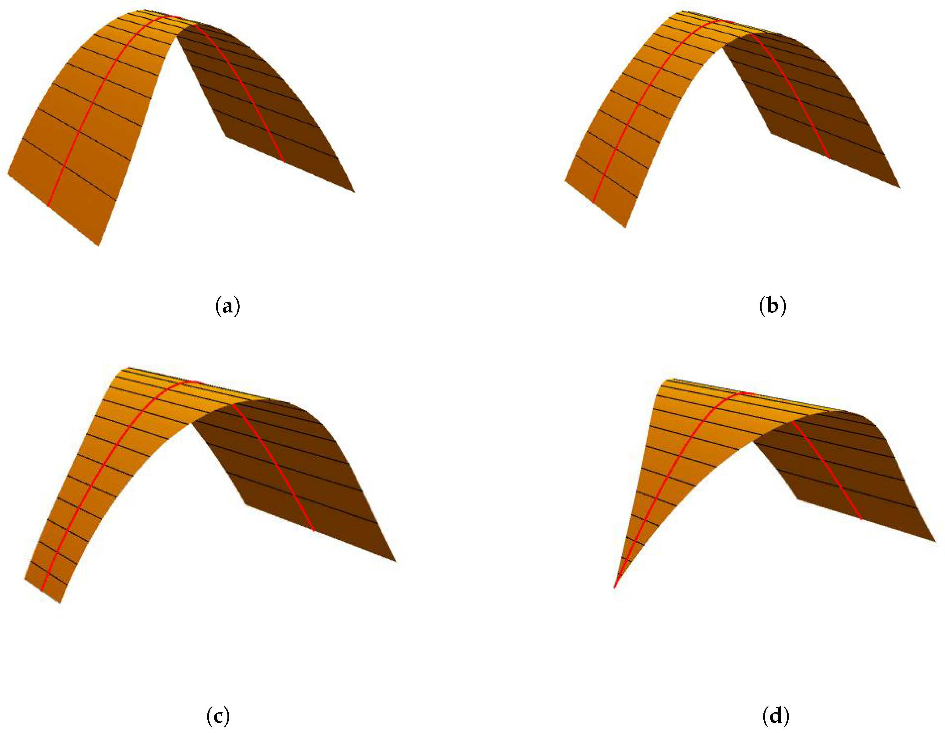
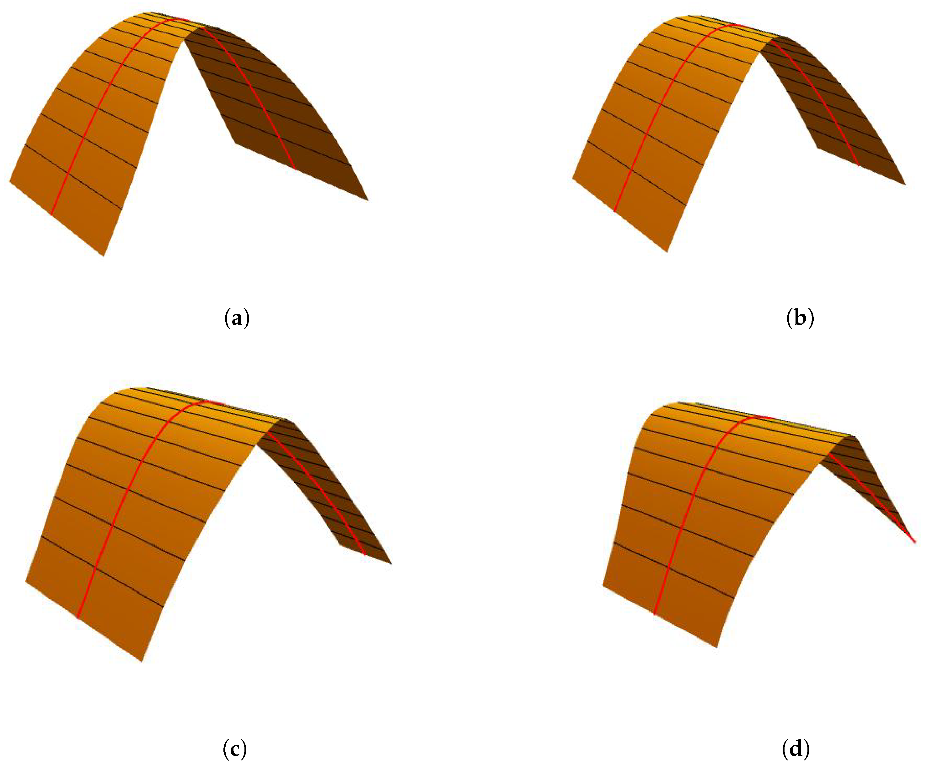
5.2. Examples of Spine Curve GDCT-Bézier Surfaces

In this example, the construction of the spine curve GDCT-Bézier surface is demonstrated. Assume the coordinates of the control planes are

$$\begin{array}{c}\begin{array}{cc}\hfill R_0=(13/2,13/2,13\sqrt{2}/2,169),& R_1=(-15/2,-15/2,13\sqrt{2}/2,225),\hfill \\ \hfill R_2=(-10,-10,10\sqrt{2},400),& R_3=(25/2,-25/2,25\sqrt{2}/2,625).\hfill \end{array}\end{array}$$

In designing the developable surface of the spine curve, we assume that the four control planes have their center points in four different quadrants and that the distance to the origin is not equivalent from these center points.

In Figure 4 and Figure 5, we can see the impact of shape parameters ${\gamma }_1$, ${\gamma }_2$ on the spine curve developable surface as follows:

• When modifying the value of ${\gamma }_1$, and keeping ${\gamma }_2$ unchanged, the $T(0;{\gamma }_1,{\gamma }_2)$ generator retains the same length and location. However, the length of the generator $T(1;{\gamma }_1,{\gamma }_2)$ becomes shorter when we increase the value of ${\gamma }_1$, but its position remains unchanged.
• If the value of shape parameter ${\gamma }_1$ is constant and ${\gamma }_2$ is adjusted, the generator $T(1;{\gamma }_1,{\gamma }_2)$ retains the same length. However, the length of the generator $T(0;{\gamma }_1,{\gamma }_2)$ becomes shorter when we increase the value of ${\gamma }_2$, but its position remains unchanged.

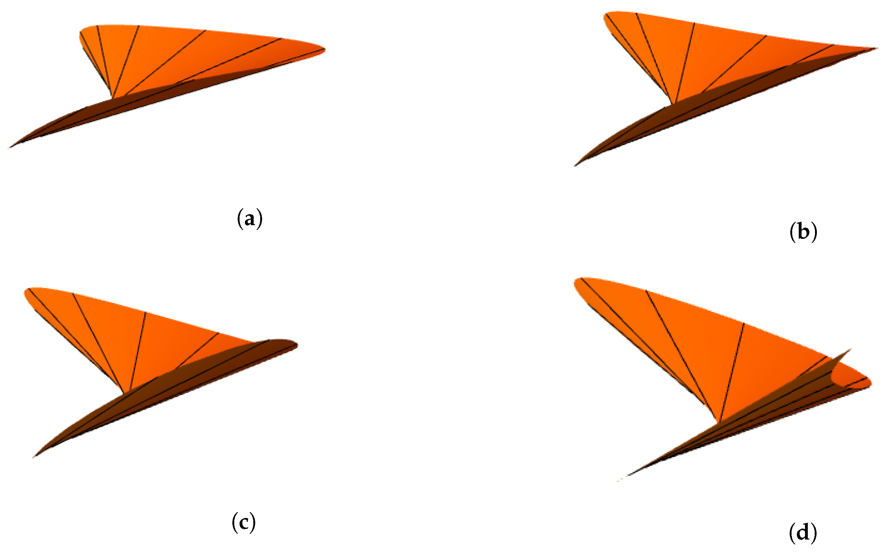
5.3. Example of Developable Surface Interpolating Geodesic Cubic Trigonometric Bézier Curve with Parameters

In order to illustrate the effectiveness of the method constructed in Section 3.4, we design a developable surface with a special case when ${\mu }_2=1$. The resulting developable surface interpolates the curve created by control points $b_0=[3,3,3],b_1=[4,3,5],b_2=[5,3,5],b_3=[6,3,3]$. Although the curve is geodesic to the developable surface, note that the shape parameters have an influence on the developable surface as shown in Figure 6 and Figure 7.

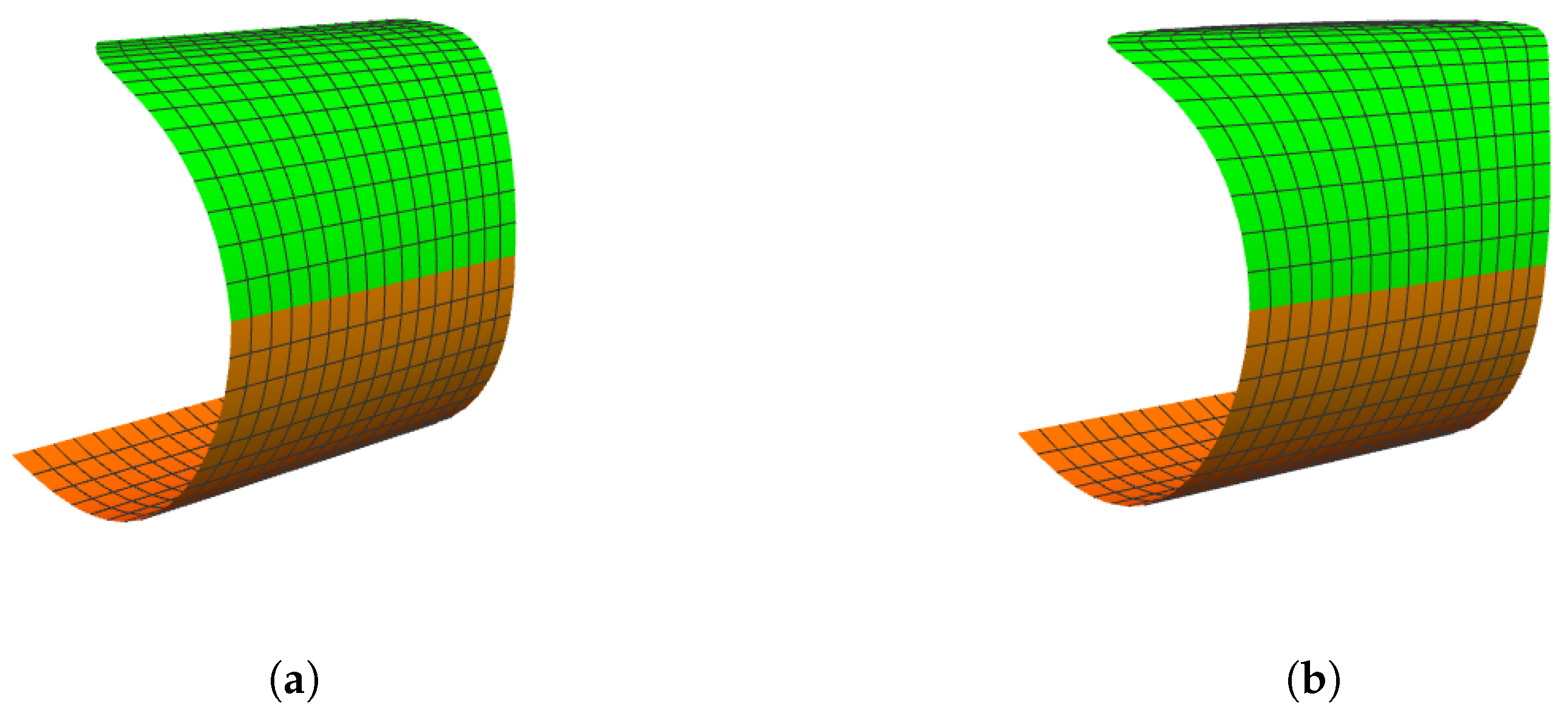
5.4. Example of Smooth Continuity Between Two Adjacent GDCT-Bézier Surfaces

In the field of Computer Aided Design, product appearance modeling is often undertaken by splicing together several developable patches. However, this paper has portrayed many dynamic surfaces being placed directly using the developable surfaces and their smooth continuity. Figure 8a,b show the $G^1$ smooth continuity example between two enveloping GDCT-Bézier surfaces. In Figure 8, the orange surface is the first enveloping GDCT-Bézier surface $S_1(u;{\gamma }_{1,1},{\gamma }_{2,1})$, whose shape parameters are ${\gamma }_{1,1}=1$,${\gamma }_{2,1}=1$ and with control planes

$$\begin{array}{c}\begin{array}{cc}\hfill R_{0,1}=(0,-17.32,10.,400),& R_{1,1}=(0,-10.,17.32,400),\hfill \\ \hfill R_{2,1}=(0,10.,17.32,400),& R_{3,1}=(0,17.32,10.,400).\hfill \end{array}\end{array}$$

The green surface is the second enveloping GDCT-Bézier surface $S_2(u;{\gamma }_{1,2},{\gamma }_{2,2})$, which satisfies $G^1$ smooth continuity with $S_1(u;{\gamma }_{1,1},{\gamma }_{2,1})$, having the control planes

$$\begin{array}{c}\begin{array}{cc}\hfill R_{0,2}=(0,17.32,10.,400),& R_{1,2}=(0,24.641,2.679,400),\hfill \\ \hfill R_{2,2}=(0,20,-13,400),& R_{3,2}=(0,15,-20,400).\hfill \end{array}\end{array}$$

When the shape parameter ${\gamma }_{1,2}=1$, the control plane coordinates $R_{0,2}$ and $R_{1,2}$ are obtained by Equation (23) with the constant value of $\varphi =1$, and the control planes $R_{2,2}$ and $R_{3,2}$ are chosen freely. According to Equation (23), ${\gamma }_{2,2}$ is independent of $G^1$ smooth continuity. Figure 8a,b show the $G^1$ piecewise enveloping developable surfaces with ${\gamma }_{1,1}=0$,${\gamma }_{2,1}=0$,${\gamma }_{1,2}=0$,${\gamma }_{2,2}=1$ and ${\gamma }_{1,1}=0$,${\gamma }_{2,1}=0$,${\gamma }_{1,2}=0$,${\gamma }_{2,2}=-2$, respectively. This concludes that the process of modeling a complex product using continuity constraints is quick and easy to control, making it easier to meet the actual need. Additionally, we are able to achieve smooth continuity between spine curve GDCT-Bézier surfaces using the same technique.

6. Conclusions

Based on the CT-Bézier basis function with two shape parameters, this article has presented a novel approach for constructing a class of GDCT-Bézier function with local control for enveloping and spine developable surfaces. Furthermore, the conditions and evaluation of some interesting properties of the GDCT-Bézier surface to create geodesic interpolating surfaces are successfully derived. The shapes of the GDCT-Bézier surfaces can be easily modified due to the inclusion of a shape parameter without changing the control planes. This suggests that the Bézier trigonometric surfaces have increased surface design efficiency with added versatility. This developable surface inherits the properties of the classical developable Bézier surface. In addition, in order to handle complex shapes in engineering and architectural design, we have also derived sufficient and necessary continuity conditions between two adjacent GDCT-Bézier surfaces. Theoretical discussion and design examples, however, suggest that the GDCT-Bézier surfaces and their smooth continuity are not only easy and convenient to integrate but also provide a great deal of flexibility in the design of developing surfaces. Thus, they are prominently useful in constructing complex developable surfaces in CAD/CAM with different degrees of smoothness. However, our future aim is to investigate the approximation and interpolation of cubic trigonometric Bézier surfaces by exploring special algorithms for developable surfaces.

References

1. Liu, Y.; Pottmann, H.; Wallner, J.; Yang, Y.L.; Wang, W. Geometric modeling with conical meshes and developable surfaces. ACM Trans. Graph. 2006, 25, 681–689. [Google Scholar] [CrossRef]
2. Tang, C.; Bo, P.; Wallner, J.; Pottmann, H. Interactive design of developable surfaces. ACM Trans. Graph. (TOG) 2016, 35, 1–12. [Google Scholar] [CrossRef]
3. Tang, K.; Wang, C.C. Modeling developable folds on a strip. J. Comput. Inf. Sci. Eng. 2005, 5, 35–47. [Google Scholar] [CrossRef] [Green Version]
4. Ferris, L.W. A standard series of developable surfaces. Mar. Technol. SNAME News 1968, 5, 52–62. [Google Scholar]
5. Frey, W.; Bindschadler, D. Computer Aided Design of a Class of Developable Bézier Surfaces; General Motors R&D Publication: Detroit, The Netherlands, 1993. [Google Scholar]
6. Chu, C.H.; Wang, C.C.; Tsai, C.R. Computer aided geometric design of strip using developable Bézier patches. Comput. Ind. 2008, 59, 601–611. [Google Scholar] [CrossRef]
7. Nguyen, H.; Ko, S.L. A mathematical model for simulating and manufacturing ball end mill. Comput. Aided Des. 2014, 50, 16–26. [Google Scholar] [CrossRef]
8. Weiss, G.; Furtner, P. Computer-aided treatment of developable surfaces. Comput. Graph. 1988, 12, 39–51. [Google Scholar] [CrossRef]
9. Chen, M.; Tang, K. G2 quasi-developable Bezier surface interpolation of two space curves. Comput. Aided Des. 2013, 45, 1365–1377. [Google Scholar] [CrossRef]
10. Peternell, M. Developable surface fitting to point clouds. Comput. Aided Geom. Des. 2004, 21, 785–803. [Google Scholar] [CrossRef]
11. Zhao, H.; Wang, G. A new method for designing a developable surface utilizing the surface pencil through a given curve. Prog. Nat. Sci. 2008, 18, 105–110. [Google Scholar] [CrossRef]
12. Li, C.Y.; Wang, R.H.; Zhu, C.G. Design and G1 connection of developable surfaces through Bézier geodesics. Appl. Math. Comput. 2011, 218, 3199–3208. [Google Scholar] [CrossRef]
13. Chu, C.H.; Chen, J.T. Geometric design of developable composite Bézier surfaces. Comput. Aided Des. Appl. 2004, 1, 531–539. [Google Scholar] [CrossRef] [Green Version]
14. Aumann, G. Interpolation with developable Bézier patches. Comput. Aided Geom. Des. 1991, 8, 409–420. [Google Scholar] [CrossRef]
15. Lang, J.; Röschel, O. Developable (1, n)-Bézier surfaces. Comput. Aided Geom. Des. 1992, 9, 291–298. [Google Scholar] [CrossRef]
16. Pottmann, H.; Farin, G. Developable rational Bézier and B-spline surfaces. Comput. Aided Geom. Des. 1995, 12, 513–531. [Google Scholar] [CrossRef]
17. Bodduluri, R.; Ravani, B. Design of developable surfaces using duality between plane and point geometries. Comput. Aided Des. 1993, 25, 621–632. [Google Scholar] [CrossRef]
18. Bobenko, A.I.; Lutz, C.; Pottmann, H.; Techter, J. Laguerre Geometry in Space Forms and Incircular Nets. 2019. Available online: https://www.discretization.de/media/filer_public/a4/f3/a4f33445-83b2-46b0-a6c2-a34e1a463531/laguerre.pdf (accessed on 21 December 2020).
19. Peternell, M.; Pottmann, H. A Laguerre geometric approach to rational offsets. Comput. Aided Geom. Des. 1998, 15, 223–249. [Google Scholar] [CrossRef]
20. Skopenkov, M.; Bo, P.; Bartoň, M.; Pottmann, H. Characterizing envelopes of moving rotational cones and applications in CNC machining. arXiv 2020, arXiv:2001.01444. [Google Scholar] [CrossRef]
21. Pottmann, H.; Grohs, P.; Mitra, N.J. Laguerre minimal surfaces, isotropic geometry and linear elasticity. Adv. Comput. Math. 2009, 31, 391. [Google Scholar] [CrossRef] [Green Version]
22. Li, C.Y.; Wang, R.H.; Zhu, C.G. An approach for designing a developable surface through a given line of curvature. Comput. Aided Des. 2013, 45, 621–627. [Google Scholar] [CrossRef]
23. Farin, G. Rational curves and surfaces. In Mathematical Methods in Computer Aided Geometric Design; Elsevier: Amsterdam, The Netherlands, 1989; pp. 215–238. [Google Scholar]
24. Piegl, L. On NURBS: A survey. IEEE Comput. Graph. Appl. 1991, 11, 55–71. [Google Scholar] [CrossRef]
25. Farin, G. From conics to NURBS: A tutorial and survey. IEEE Comput. Graph. Appl. 1992, 12, 78–86. [Google Scholar] [CrossRef]
26. Han, X. Quadratic trigonometric polynomial curves with a shape parameter. Comput. Aided Geom. Des. 2002, 19, 503–512. [Google Scholar] [CrossRef]
27. Wu, B.; Yin, J.; Li, C. A New Rational Cubic Trigonometric Bézier Curve with Four Shape Parameters. J. Inf. Comput. Sci. 2015, 12, 7023–7029. [Google Scholar] [CrossRef]
28. Majeed, A.; Qayyum, F. New rational cubic trigonometric B-spline curves with two shape parameters. Comput. Appl. Math. 2020, 39, 1–24. [Google Scholar] [CrossRef]
29. Majeed, A.; Abbas, M.; Qayyum, F.; Miura, K.T.; Misro, M.Y.; Nazir, T. Geometric Modeling Using New Cubic Trigonometric B-spline Functions with Shape Parameter. Mathematics 2020, 8, 2102. [Google Scholar] [CrossRef]
30. Bashir, U.; Abbas, M.; Ali, J.M. The quartic trigonometric Bézier curve with two shape parameters. In Proceedings of the 2012 Ninth International Conference on Computer Graphics, Imaging and Visualization, Hsinchu, Taiwan, 25–27 July 2012; pp. 70–75. [Google Scholar]
31. Yang, L.; Li, J.; Chen, Z. Trigonometric extension of quartic Bézier curves. In Proceedings of the 2011 International Conference on Multimedia Technology, Hangzhou, China, 26–28 July 2011; pp. 926–929. [Google Scholar]
32. Misro, M.Y.; Ramli, A.; Ali, J.M. Quintic trigonometric Bézier curve with two shape parameters. Sains Malays. 2017, 46, 825–831. [Google Scholar]
33. Misro, M.Y.; Ramli, A.; Ali, J.M.; Hamid, N.N.A. Pythagorean hodograph quintic trigonometric Bézier transtion curve. In Proceedings of the 2017 14th International Conference on Computer Graphics, Imaging and Visualization, Marrakesh, Morocco, 23–25 May 2017; pp. 1–7. [Google Scholar]
34. Misro, M.Y.; Ramli, A.; Ali, J.M. Quintic trigonometric Bézier curve and its maximum speed estimation on highway designs. AIP Conf. Proc. 2018, 1974, 020089. [Google Scholar]
35. Ammad, M.; Misro, M.Y. Construction of Local Shape Adjustable Surfaces Using Quintic Trigonometric Bézier Curve. Symmetry 2020, 12, 1205. [Google Scholar] [CrossRef]
36. Hu, G.; Cao, H.; Qin, X. Construction of generalized developable Bézier surfaces with shape parameters. Math. Methods Appl. Sci. 2018, 41, 7804–7829. [Google Scholar] [CrossRef]
37. Hu, G.; Wu, J.; Qin, X. A new approach in designing of local controlled developable H-Bézier surfaces. Adv. Eng. Softw. 2018, 121, 26–38. [Google Scholar] [CrossRef]
38. BiBi, S.; Abbas, M.; Misro, M.Y.; Hu, G. A Novel Approach of Hybrid Trigonometric Bézier Curve to the Modeling of Symmetric Revolutionary Curves and Symmetric Rotation Surfaces. IEEE Access 2019, 7, 165779–165792. [Google Scholar] [CrossRef]
39. BiBi, S.; Abbas, M.; Miura, K.T.; Misro, M.Y. Geometric Modeling of Novel Generalized Hybrid Trigonometric Bézier-Like Curve with Shape Parameters and Its Applications. Mathematics 2020, 8, 967. [Google Scholar] [CrossRef]
40. Han, X.A.; Ma, Y.; Huang, X. The cubic trigonometric Bézier curve with two shape parameters. Appl. Math. Lett. 2009, 22, 226–231. [Google Scholar] [CrossRef] [Green Version]
41. Do Carmo, M.P. Differential Geometry of Curves and Surfaces; Prentice-Hall: Upper Saddle River, NJ, USA, 1976; pp. 5–7. [Google Scholar]
42. Li, C.Y.; Zhu, C.G. G1 continuity of four pieces of developable surfaces with Bézier boundaries. J. Comput. Appl. Math. 2018, 329, 164–172. [Google Scholar] [CrossRef]
43. Farin, G.E.; Farin, G. Curves and Surfaces for CAGD: A Practical Guide; Morgan Kaufmann: Burlington, MA, USA, 2002. [Google Scholar]
44. Zhou, M.; Yang, J.; Zheng, H.; Song, W. Design and shape adjustment of developable surfaces. Appl. Math. Model. 2013, 37, 3789–3801. [Google Scholar] [CrossRef]
45. Hwang, H.D.; Yoon, S.H. Constructing developable surfaces by wrapping cones and cylinders. Comput. Aided Des. 2015, 58, 230–235. [Google Scholar] [CrossRef]
46. Liu, Y.J.; Lai, Y.K.; Hu, S. Stripification of free-form surfaces with global error bounds for developable approximation. IEEE Trans. Autom. Sci. Eng. 2009, 6, 700–709. [Google Scholar]
47. Liu, Y.J.; Tang, K.; Joneja, A. Modeling dynamic developable meshes by the Hamilton principle. Comput. Aided Des. 2007, 39, 719–731. [Google Scholar] [CrossRef]
48. Liu, Y.J.; Tang, K.; Gong, W.Y.; Wu, T.R. Industrial design using interpolatory discrete developable surfaces. Comput. Aided Des. 2011, 43, 1089–1098. [Google Scholar] [CrossRef]
49. Jüttler, B.; Sampoli, M.L. Hermite interpolation by piecewise polynomial surfaces with rational offsets. Comput. Aided Geom. Des. 2000, 17, 361–385. [Google Scholar] [CrossRef]
50. Han, X.A.; Ma, Y.; Huang, X. A novel generalization of Bézier curve and surface. J. Comput. Appl. Math. 2008, 217, 180–193. [Google Scholar] [CrossRef] [Green Version]
Figure 1. Cubic trigonometric (CT)-Bézier basis functions for different combinations of shape parameters. (a) γ 1 = 1 , γ 2 = 1 , (b) γ 1 = 1 , γ 2 = 1 , (c) γ 1 = 1 , γ 2 = 1 , (d) γ 1 = 2 , γ 2 = 2 .
Mathematics 09 00283 g001
Figure 2. The effect of parameter γ 1 on the 1 × 3 enveloping developable surface (a) γ 1 = 1 , γ 2 = 1 , (b) γ 1 = 0 , γ 2 = 1 , (c) γ 1 = 1 , γ 2 = 1 , (d) γ 1 = 2 , γ 2 = 1 .
Mathematics 09 00283 g002
Figure 3. The effect of parameter γ 2 on the 1 × 3 enveloping developable surface (a) γ 1 = 1 , γ 2 = 1 , (b) γ 1 = 1 , γ 2 = 0 , (c) γ 1 = 1 , γ 2 = 1 (d) γ 1 = 1 , γ 2 = 2 .
Mathematics 09 00283 g003
Figure 4. The effects of parameter γ 1 on the 1 × 3 tangent of the spine curve developable surface (a) γ 1 = 0 , γ 2 = 0 , (b) γ 1 = 0.7 , γ 2 = 0 , (c) γ 1 = 1.4 , γ 2 = 0 , (d) γ 1 = 2 , γ 2 = 0 .
Mathematics 09 00283 g004
Figure 5. The effects of parameter γ 2 on the 1 × 3 tangent of the spine curve developable surface (a) γ 1 = 0 , γ 2 = 0 , (b) γ 1 = 0 , γ 2 = 0.7 , (c) γ 1 = 0 , γ 2 = 1.4 , (d) γ 1 = 0 , γ 2 = 2 .
Mathematics 09 00283 g005
Figure 6. The effects of parameter γ 1 on the developable surface through the geodesic (a) γ 1 = 1 , γ 2 = 1 , (b) γ 1 = 0 , γ 2 = 1 , (c) γ 1 = 1 , γ 2 = 1 , (d) γ 1 = 2 , γ 2 = 1 .
Mathematics 09 00283 g006
Figure 7. The effects of parameter γ 2 on the developable surface through the geodesic (a) γ 1 = 1 , γ 2 = 1 , (b) γ 1 = 1 , γ 2 = 0 , (c) γ 1 = 1 , γ 2 = 1 , (d) γ 1 = 1 , γ 2 = 2 .
Mathematics 09 00283 g007
Figure 8. G 1 smooth continuity between two enveloping generalized developable cubic trigonometric (GDCT)-Bézier surfaces. (a) γ 1 , 1 = 0 , γ 2 , 1 = 0 , γ 1 , 2 = 0 , γ 2 , 2 = 1 , (b) γ 1 , 1 = 0 , γ 2 , 1 = 0 , γ 1 , 2 = 0 , γ 2 , 2 = 2 .
Mathematics 09 00283 g008
Publisher’s Note: MDPI stays neutral with regard to jurisdictional claims in published maps and institutional affiliations.