Spline Curves Formation Given Extreme Derivatives

Abstract

This paper is dedicated to development of mathematical models for polynomial spline curve formation given extreme vector derivatives. This theoretical problem is raised in the view of a wide variety of theoretical and practical problems considering motion of physical objects along certain trajectories with predetermined laws of variation of speed, acceleration, jerk, etc. The analysis of the existing body of work on computational geometry performed by the authors did not reveal any systematic research in mathematical model development dedicated to solution of similar tasks. The established purpose of the research is therefore to develop mathematical models of formation of spline curves based on polynomials of various orders modeling the determined trajectories. The paper presents mathematical models of spline curve formation given extreme derivatives of the initial orders. The paper considers construction of Hermite and Bézier spline curves of various orders consisting of various segments. The acquired mathematical models are generalized for the cases of vector derivatives of higher orders. The presented models are of systematic nature and are universal, i.e., they can be applied in formation of any polynomial spline curves given extreme vector derivatives. The paper provides a number of examples validating the presented models.

1. Introduction

Formation of composite polynomial spline curves given the initial extreme derivatives at the endpoints of the segments is finding increasing application in solutions to a variety of tasks of science and manufacture. For example, in computer animation, camera motion along a curvilinear trajectory is modeled as motion along a curved line $\overline{r}(t)$, $t_1\le t\le t_2$. Camera trajectory calculation is performed with consideration for laws of variation of camera velocity $\overline{v}(t)=\frac{d\overline{r}}{dt}$ and acceleration $\overline{a}(t)=\frac{d\overline{v}}{dt}=\frac{d^2\overline{r}}{d{t}^2}$ throughout the trajectory [1].

In machine-building cutting tool trajectory calculation through Hermite cubic spline interpolation is applied in pocket machining of surfaces of arbitrary shape. In this regard, it is noted that that cutting tool acceleration is not continuous, which results in machining defects [2].

One of the main problems in development of high-speed cutting NC systems is achieving seamless cutting tool motion. The models of NC systems developed for this purpose ensure smoothness of acceleration $\overline{a}(t)$ and continuity of jerk defined by the third vector derivative [3,4,5]: $\overline{j}=\frac{d\overline{a}}{dt}=\frac{d^3\overline{r}}{d{t}^3}$.

The fourth vector derivative is called snap $\frac{d\overline{j}}{dt}=\frac{d^4\overline{r}}{d{t}^4}$. It is applied, for example, in development of minimum snap trajectory for quadrotors [6].

Papers [7,8] apply the sixth vector derivative in Apophis asteroid trajectory calculation in Earth gravity field.

As follows from the mentioned papers, spline curve formation through extreme derivatives $S{C}_{ED}^{(n)}$ (spline curve extreme derivative of nth order) is relevant in solution to a variety of practical tasks.

There are approaches to development of mathematical models of $S{C}_{ED}^{(n)}$ formation known from scientific papers on spline curve theory. One should trace the origins of this development to cubic spline interpolation through formation of Hermite segments given first-order extreme derivatives subsequently connected with smoothness $C^2$ into cubic $S{C}_{ED}^{(3)}$ [1,9,10,11,12,13,14,15,16,17,18,19]. The $S{C}_{ED}^{(3)}$ model later became the basis for development of mathematical model of a Hermite segment $SC{S}_{ED}^{(5)}$ (spline curve segment) described by a polynomial of the fifth order given the extreme derivatives of the first and the second order [1]. However, in subsequent formation of the $S{C}_{ED}^{(5)}$ mathematical model, the first and the second vector derivatives at the first point of the first segment and at the final point of the final segment were not initially specified, therefore the mathematical model resulted in a system of linear equations with the number of unknown values exceeding the number of equations. In the course of development of this system, the fact that it is incomplete has been revealed. The author of paper [1] made a decision to reduce the number of unknown values down to the number of equations by assigning values to certain extreme vector derivatives. The resultant approach to solution of the problem of $S{C}^{(5)}$ formation is of purely theoretical nature. In practice, the more relevant approach is $S{C}_{ED}^{(5)}$ formation. According to this approach, both the segment $SC{S}_{ED}^{(5)}$ and the composite curve $S{C}_{ED}^{(5)}$ acquired through connection of segments with smoothness $C^4$ are formed through the same mathematical model.

We have to acknowledge the paper of theoretical nature proposing a mathematical model of $S{C}_{ED}^{(3)}$ and $S{C}_{ED}^{(4)}$ formation in the form of B-spline curves interpolating discrete arrays of points in the plane [20]. The paper considers vector derivatives of orders one to three as given extreme derivatives. It is noted that the problem of spatial interpolation with consideration for curvature and torsion in order to acquire $S{C}_{ED}$ does not yet have a solution. In this regard, the authors of the paper [20] provide an explanation that it is virtually impossible to evaluate corresponding directions and magnitudes of vectors of the second and the third derivative in $S{C}_{ED}$ formation. We were unable to find more modern papers in this area of research.

Therefore, with regard for practical requirements in models and algorithms for formation of curves $S{C}_{ED}^{(n)}$, $n>3$ and taking into account the existing theoretical basis of mathematical models of spline curves, the following purpose of the research is established: to develop mathematical models of formation of polynomial curves $S{C}_{ED}^{(n)}$, $n>3$ and to validate these models on numeric experiments.

Section 2 of the present paper considers the conditions for formation of spline curves given extreme derivatives of the initial orders and provides generalizations for the case of first $k$ vector derivatives.

Section 3 considers the mathematical models and many examples for closed and non-closed polynomial spline curves of various orders and consisting of various numbers of segments.

2. Conditions for Spline Curve Formation Given Extreme Derivatives

At the initial stage of analytical spline curve shaping given extreme derivatives it is essential to know the total number of conditions for shaping. Knowing the total number of conditions allows one to determine the degree of a polynomial describing the segment—or each segment—of the desired spline curve.

2.1. Conditions for Hermite Cubic Sspline Curve Shaping

It is known that a cubic spline segment can be constructed given boundary conditions ${\overline{P}}_1$, ${\overline{P}}_1^{\prime }$ and ${\overline{P}}_2$, ${\overline{P}}_2^{\prime }$ [1,9,10,11,12,13,14,15,16,17,18,19] (see Figure 1).

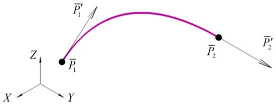
Figure 1. Hermitian cubic segment.

In the general case, the order of polynomial describing the segment through extreme derivatives is determined through formula $n=2m+1$, where $m$ represents the number of pairs of extreme derivatives at segment endpoints. As follows from the technique of algebraic definition of polynomial coefficients of cubic spline $\overline{p}(t)={\displaystyle \sum _{i=1}^4{\overline{A}}_i}{t}^{i-1}$, $t_1\le t\le t_2$, the existence of four boundary conditions resulting in respective algebraic equations is sufficient for unambiguous definition of four coefficients of the polynomial.

Eight conditions defining four vector coefficients of each polynomial describing a segment are required in order to define a cubic spline curve consisting of two segments. These conditions include the given boundary conditions ${\overline{P}}_1$, ${\overline{P}}_1^{\prime }$; ${\overline{P}}_3$, ${\overline{P}}_3^{\prime }$, and intermediate conditions in connection point ${\overline{P}}_2$ (see Figure 2): ${\overline{P}}_2={\overline{p}}_1(t=t_2)$, ${\overline{P}}_2={\overline{p}}_2(t=0)$; ${\overline{P}}_2^{\prime }={\overline{p}}_1^{\prime }(t=t_2)$, ${\overline{P}}_2^{\prime }={\overline{p}}_2^{\prime }(t=0)$, where ${\overline{p}}_1(t)$ and ${\overline{p}}_2(t)$ are polynomials of respective segments $s_1$ and $s_2$.

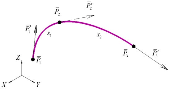
Figure 2. Two-segment Hermite cubic spline curve.

As follows from the intermediate conditions, the point ${\overline{P}}_2$ should be considered double as well as the unknown derivative ${\overline{P}}_2^{\prime }$ at that point. Each boundary and intermediate condition is described by a linear algebraic equation. Simultaneously, these equations unambiguously define the unknown coefficients of the polynomials of the connected segments. A general cubic spline curve consisting of $(j-1)$ segments, where $j$ is the number of points of the curve, is formed through a total number of $N$ conditions, where $N$ is obviously defined through formula $N=4(j-1)$. This number is also the total number of the unknown coefficients of all polynomials of the third degree describing the connected segments.

2.2. Conditions for Formation of a Spline Curve of Segments Described by Polynomials of Higher Degree

A segment with two pairs of extreme derivatives (see Figure 3) is described, according to the formula $n=2m+1$, by a polynomial of the fifth degree $\overline{p}(t)={\displaystyle \sum _{i=1}^6{\overline{A}}_i}{t}^{i-1}$, $t_1\le t\le t_2$. Six conditions ${\overline{P}}_1$, ${\overline{P}}_1^{\prime }$, ${\overline{P}}_1^{″}$; ${\overline{P}}_2$, ${\overline{P}}_2^{\prime }$, ${\overline{P}}_2^{″}$ unambiguously define six coefficients of this polynomial [1].

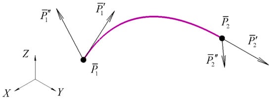
Figure 3. Hermitian fifth-degree segment.

Formation of a spline curve consisting of two segments defined by fifth-degree polynomials requires 12 conditions. These conditions include the given boundary conditions ${\overline{P}}_1$, ${\overline{P}}_1^{\prime }$, ${\overline{P}}_1^{″}$; ${\overline{P}}_3$, ${\overline{P}}_3^{\prime }$, ${\overline{P}}_3^{″}$; the intermediate conditions in connection point ${\overline{P}}_2$ (see Figure 4): ${\overline{P}}_2={\overline{p}}_1(t=t_2)$, ${\overline{P}}_2={\overline{p}}_2(t=0)$; ${\overline{P}}_2^{\prime }={\overline{p}}_1^{\prime }(t=t_2)$, ${\overline{P}}_2^{\prime }={\overline{p}}_2^{\prime }(t=0)$; ${\overline{P}}_2^{″}={\overline{p}}_1^{″}(t=t_2)$, ${\overline{P}}_2^{″}={\overline{p}}_2^{″}(t=0)$, where ${\overline{p}}_1(t)$ and ${\overline{p}}_2(t)$ are polynomials of the fifth degree of respective segments $s_1$ and $s_2$.

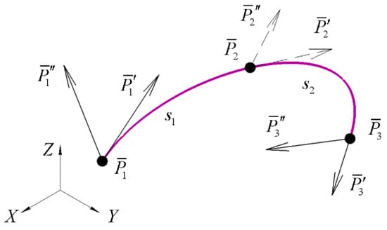
Figure 4. Fifth-degree Hermite spline curve of two segments.

Obviously, the point ${\overline{P}}_2$ should be considered double, as well as the first- and the second-order derivatives at it. The algorithms of formation of Hermite spline curves based on fifth-degree and seventh-degree polynomials are thoroughly considered in Section 3.1, Section 3.2, Section 3.3, Section 3.4 and Section 3.5 respectively.

Formation of a general spline curve consisting of $(j-1)$ smoothly connected segments defined by fifth-degree polynomials requires the total number of $N=6(j-1)$ conditions. This number is also the total number of the unknown coefficients of all fifth-degree polynomials describing $(j-1)$ segments.

If we consider two given points ${\overline{P}}_1$ and ${\overline{P}}_2$, as well as the first $k$ vector derivatives at each point, then, according to the formula $n=2m+1$, the degree of the polynomial defining a segment with endpoints ${\overline{P}}_1$ and ${\overline{P}}_2$ equals $n=2k+1$. It is possible to define the total number of conditions for formation of a general spline curve consisting of $(j-1)$ segments each described by a polynomial of degree $2k+1$. It is calculated through the formula $N=2(k+1)(j-1)$. Thus, for example, if $k=2$ and $j=3$, $N=12$, which correlates to the spline curve depicted on Figure 4.

2.3. Conditions for Closed Spline Curve Formation

In order to form a closed spline curve given a discrete array of $j$ points, it is required to fulfill the total number of $N=2(k+1)j$ conditions. Here $k$ represents the number of pairs of extreme derivatives of the initial orders at the endpoints of the formed spline curve, $j$ represents the number of segments. For example, given four points ${\overline{P}}_j$, $j=1,\dots ,4$ with respective derivatives ${\overline{P}}_j^{\prime }$, ${\overline{P}}_j^{″}$ it is possible to form a closed Hermite spline curve based on a fifth-degree polynomial (see Figure 5). The resultant curve consists of four segments connected with smoothness $C^4$.

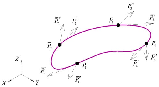
Figure 5. Closed spline curve based on a fifth-degree polynomial.

Obviously, the total number of conditions defining this spline curve equals $N=24$, i.e., six conditions for each segment of the curve. Let us list them: the boundary (given) conditions ${\overline{P}}_1$,… ${\overline{P}}_4$, whereby ${\overline{P}}_1={\overline{p}}_4(t=t_4)$, ${\overline{P}}_1={\overline{p}}_1(t=0)$; ${\overline{P}}_2={\overline{p}}_1(t=t_1)$, ${\overline{P}}_2={\overline{p}}_2(t=0)$; ${\overline{P}}_3={\overline{p}}_2(t=t_2)$, ${\overline{P}}_3={\overline{p}}_3(t=0)$; ${\overline{P}}_4={\overline{p}}_3(t=t_3)$, ${\overline{P}}_4={\overline{p}}_4(t=0)$; $0\le t\le t_j$; the intermediate (sought) conditions in the segments connection points are as follows: ${\overline{P}}_1^{\prime }={\overline{p}}_4^{\prime }(t=t_4)$, ${\overline{P}}_1^{\prime }={\overline{p}}_1^{\prime }(t=0)$, ${\overline{P}}_2^{\prime }={\overline{p}}_1^{\prime }(t=t_1)$, ${\overline{P}}_2^{\prime }={\overline{p}}_2^{\prime }(t=0)$, ${\overline{P}}_3^{\prime }={\overline{p}}_2^{\prime }(t=t_2)$, ${\overline{P}}_3^{\prime }={\overline{p}}_3^{\prime }(t=0)$, ${\overline{P}}_4^{\prime }={\overline{p}}_3^{\prime }(t=t_3)$, ${\overline{P}}_4^{\prime }={\overline{p}}_4^{\prime }(t=0)$; ${\overline{P}}_1^{″}={\overline{p}}_4^{″}(t=t_4)$, ${\overline{P}}_1^{″}={\overline{p}}_1^{″}(t=0)$, ${\overline{P}}_2^{″}={\overline{p}}_1^{″}(t=t_1)$, ${\overline{P}}_2^{″}={\overline{p}}_2^{″}(t=0)$, ${\overline{P}}_3^{″}={\overline{p}}_2^{″}(t=t_2)$, ${\overline{P}}_3^{″}={\overline{p}}_3^{″}(t=0)$, ${\overline{P}}_4^{″}={\overline{p}}_3^{″}(t=t_3)$, ${\overline{P}}_4^{″}={\overline{p}}_4^{″}(t=0)$.

Obviously, in formation of a polynomial closed spline curve each point of the given discrete array is considered double, as well as each defined vector derivative at any point of the array. The formation of closed polynomial splines is thoroughly considered on examples in Section 3.3 and Section 3.7.

3. Spline Curve Formation Given Extreme Derivatives

In the following section let us consider the construction of mathematical models of polynomial spline curves consisting of various numbers of smoothly connected segments. The segmental formation of spline curves is based on the concept of a continuous (or smooth) connection of segments at their common point. In the theory of spline curves and spline surfaces two types of smoothness are known: geometric $G^n$ and parametric $G^n$ [1,9,13]. Within the framework of this work, we use the strict concept of $C^n$ smoothness.

3.1. Construction of a Hermite Segment Given First- and Second-Order Extreme Derivatives

Let us assume the points ${\overline{P}}_1(x_1,y_1,z_1)$ and ${\overline{P}}_2(x_2,y_2,z_2)$, as well as respective boundary conditions ${\overline{P}}_1^{\prime }$, ${\overline{P}}_1^{″}$ and ${\overline{P}}_2^{\prime }$, ${\overline{P}}_2^{″}$ are given (see Figure 6).

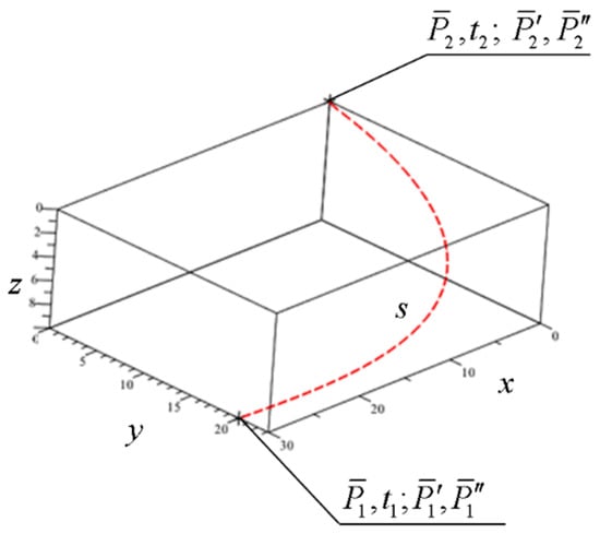
Figure 6. Initial conditions for construction of a fifth-degree Hermite spline curve segment.

Let us construct a Hermite spline curve segment $\overline{p}(t)={\displaystyle \sum _{i=1}^n{\overline{A}}_i}{t}^{i-1}$, $t_1\le t\le t_2$ passing through the points ${\overline{P}}_1$, ${\overline{P}}_2$ and conforming to the given boundary conditions. Given the two endpoints and the initial m pairs of derivatives in the endpoints, it is possible to calculate the interpolating polynomial of order 2m + 1. It is therefore obvious that the sought segment has to be described by a fifth-order polynomial

$$\overline{p}(t)={\displaystyle \sum _{i=1}^6{\overline{A}}_i}{t}^{i-1},t_1\le t\le t_2.$$

(1)

The vectors ${\overline{P}}_1^{\prime }$, ${\overline{P}}_2^{\prime }$ are the first vector derivatives constituting tangent vectors at the endpoints of the sough segment s, while ${\overline{P}}_1^{″},{\overline{P}}_2^{″}$ are the second vector derivatives constituting vectors of acceleration of a point tracing out the segment s. Obviously, the given conditions are sufficient in order to define the vector coefficients ${\overline{A}}_i$ of the Formula (1).

Let us express the equations for the vector coefficients in the final matrix form $\left[\overline{A}\right]=\left[T\right]\cdot \left[\overline{G}\right]$:

$$\left[\overline{A}\right]=\left[\begin{array}{c}{\overline{A}}_1\\ {\overline{A}}_2\\ {\overline{A}}_3\\ {\overline{A}}_4\\ {\overline{A}}_5\\ {\overline{A}}_6\end{array}\right]=\left[\begin{array}{cccccc}1& 0& 0& 0& 0& 0\\ 0& 0& 1& 0& 0& 0\\ 0& 0& 0& 0& \frac{1}{2}& 0\\ -10& 10& -6& -4& -\frac{3}{2}& \frac{1}{2}\\ 15& -15& 8& 7& \frac{3}{2}& -1\\ -6& 6& -3& -3& -\frac{1}{2}& \frac{1}{2}\end{array}\right]\cdot \left[\begin{array}{c}{\overline{P}}_1\\ {\overline{P}}_2\\ {\overline{P}}_1^{\prime }\\ {\overline{P}}_2^{\prime }\\ {\overline{P}}_1^{″}\\ {\overline{P}}_2^{″}\end{array}\right].$$

(2)

The matrix Formula (2) of equations defining the vector coefficients of a fifth-degree polynomial describing a Hermite segment corresponds to the known matrix form by D. Solomon [1]. The Formula (2) is the basis for computational algorithms of spline curve formation considered further in the present paper. By substitution of the values of vector coefficients (2) into the Formula (1) we acquire the sought equation of Hermite spline curve segment with parameterization $0\le t\le 1$.

3.2. Construction of a Fifth-Degree Hermite Spline Curve of Two Segments and Generalization for the Case of (j − 1) Segments

Let us consider the connection of two Hermite segments $s_1$ and $s_2$ (see Figure 7) given the same boundary conditions as for the previously considered case of one segment s.

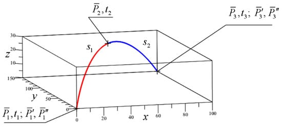
Figure 7. Calculated fifth-degree Hermite spline curve of two segments.

Parameterization of the segments is fulfilled in range $t_1\le t\le t_2$ for the segment $s_1$ and $t_2\le t\le t_3$ for the segment $s_2$. Without loss of generality, we accept that $t_1=0$ at the initial point of segment $s_1$ and $t_2=0$ at the initial point of segment $s_2$. Let us express the polynomial equation of the segments in the following form: ${\overline{p}}_k(t)={\displaystyle \sum _{i=1}^6{\overline{A}}_i^{(k)}}{t}^{i-1};k=1,2$. Let us express the derivatives of vector function ${\overline{p}}_k(t)$

$$\begin{array}{c}{\overline{p}}_k^{\prime }(t)={\displaystyle \sum _{i=2}^6{\overline{A}}_i^{(k)}(i-1)}{t}^{i-2},{\overline{p}}_k^{″}(t)={\displaystyle \sum _{i=3}^6{\overline{A}}_i^{(k)}(i-1)(i-2)}{t}^{i-3},\\ {\overline{p}}_k^{‴}(t)={\displaystyle \sum _{i=4}^6{\overline{A}}_i^{(k)}(i-1)(i-2)(i-3)}{t}^{i-4},{\overline{p}}_k^{⁗}(t)={\displaystyle \sum _{i=5}^6{\overline{A}}_i^{(k)}(i-1)(i-2)(i-3)}(i-4)t^{i-5}.\end{array}$$

For $k=1$ at the initial point ${\overline{P}}_1(t_1=0)$ of segment $s_1$ we acquire

$${\overline{p}}_1(0)={\overline{P}}_1={\overline{A}}_1^{(1)},{\overline{p}}_1^{\prime }(0)={\overline{P}}_1^{\prime }={\overline{A}}_2^{(1)},{\overline{p}}_1^{″}(0)={\overline{P}}_1^{″}=2{\overline{A}}_3^{(1)}.$$

(3)

At the final point ${\overline{P}}_2(t_2)$ of segment $s_1$ we acquire

$${\overline{p}}_1(t_2)={\overline{P}}_2={\displaystyle \sum _{i=1}^6{\overline{A}}_i^{(1)}}{t}_2^{i-1},{\overline{p}}_1^{\prime }(t_2)={\overline{P}}_2^{\prime }={\displaystyle \sum _{i=2}^6{\overline{A}}_i^{(1)}(i-1)}{t}_2^{i-2},{\overline{p}}_1^{″}(t_2)={\overline{P}}_2^{″}={\displaystyle \sum _{i=3}^6{\overline{A}}_i^{(1)}(i-1)(i-2)}{t}_2^{i-3}.$$

For $k=2$ at the initial point ${\overline{P}}_2(t_2=0)$ of segment $s_2$ we acquire

$${\overline{p}}_2(0)={\overline{P}}_2={\overline{A}}_1^{(2)},{\overline{p}}_2^{\prime }(0)={\overline{P}}_2^{\prime }={\overline{A}}_2^{(2)},{\overline{p}}_2^{″}(0)={\overline{P}}_2^{″}=2{\overline{A}}_3^{(2)}.$$

(4)

At the final point $P_3(t_3)$ of segment $s_2$ we acquire

$${\overline{p}}_2(t_3)={\overline{P}}_3={\displaystyle \sum _{i=1}^6{\overline{A}}_i^{(2)}}{t}_3^{i-1},{\overline{p}}_2^{\prime }(t_3)={\overline{P}}_3^{\prime }={\displaystyle \sum _{i=2}^6{\overline{A}}_i^{(2)}(i-1)}{t}_3^{i-2},{\overline{p}}_1^{″}(t_3)={\overline{P}}_3^{″}={\displaystyle \sum _{i=3}^6{\overline{A}}_i^{(2)}(i-1)(i-2)}{t}_3^{i-3}.$$

Thus, through (3), we acquire the expressions for the first three coefficients of the equation for the first segment $s_1$: ${\overline{A}}_1^{(1)}={\overline{P}}_1,{\overline{A}}_2^{(1)}={\overline{P}}_1^{\prime },{\overline{A}}_3^{(1)}=\frac{1}{2}{\overline{P}}_1^{″}.$ The remaining vector coefficients ${\overline{A}}_4^{(1)},{\overline{A}}_5^{(1)},{\overline{A}}_6^{(1)}$ are determined through the system of three linear equations

$$\{\begin{array}{l}{\displaystyle \sum _{i=1}^6{\overline{A}}_i^{(1)}}{t}_2^{i-1}-{\overline{P}}_2=0,\\ {\displaystyle \sum _{i=2}^6{\overline{A}}_i^{(1)}(i-1)}{t}_2^{i-2}-{\overline{P}}_2^{\prime }=0,\\ {\displaystyle \sum _{i=3}^6{\overline{A}}_i^{(1)}(i-1)(i-2)}{t}_2^{i-3}-{\overline{P}}_2^{″}=0.\end{array}$$

(5)

The expressions of the first three vector coefficients of segment $s_2$ follow from (4): ${\overline{A}}_1^{(2)}={\overline{P}}_2,{\overline{A}}_2^{(2)}={\overline{P}}_2^{\prime },{\overline{A}}_3^{(2)}=\frac{1}{2}{\overline{P}}_2^{″}.$ The remaining vector coefficients ${\overline{A}}_4^{(2)},{\overline{A}}_5^{(2)}$ and ${\overline{A}}_6^{(2)}$ are determined through the system of three linear equations

$$\{\begin{array}{l}{\displaystyle \sum _{i=1}^6{\overline{A}}_i^{(2)}}{t}_3^{i-1}-{\overline{P}}_3=0,\\ {\displaystyle \sum _{i=2}^6{\overline{A}}_i^{(2)}(i-1)}{t}_3^{i-2}-{\overline{P}}_3^{\prime }=0,\\ {\displaystyle \sum _{i=3}^6{\overline{A}}_i^{(2)}(i-1)(i-2)}{t}_3^{i-3}-{\overline{P}}_3^{″}=0.\end{array}.$$

(6)

The equations for these coefficients are of the following expanded form

$$\begin{gathered} {\overline{A}}_4^{(2)}=-\frac{10({\overline{P}}_2-{\overline{P}}_3)}{t_3^3}-\frac{6{\overline{P}}_2^{\prime }}{t_3^2}-\frac{4{\overline{P}}_3^{\prime }}{t_3^2}-\frac{1.5{\overline{P}}_2^{″}}{t_3}+\frac{0.5{\overline{P}}_3^{″}}{t_3}, \\ {\overline{A}}_5^{(2)}=\frac{15({\overline{P}}_2-{\overline{P}}_3)}{t_3^4}+\frac{8{\overline{P}}_2^{\prime }}{t_3^3}+\frac{7{\overline{P}}_3^{\prime }}{t_3^3}+\frac{1.5{\overline{P}}_2^{″}}{t_3^2}-\frac{{\overline{P}}_3^{″}}{t_3^2}, \\ {\overline{A}}_6^{(2)}=-\frac{6({\overline{P}}_2-{\overline{P}}_3)}{t_3^5}-\frac{3{\overline{P}}_2^{\prime }}{t_3^4}-\frac{3{\overline{P}}_3^{\prime }}{t_3^4}-\frac{0.5{\overline{P}}_2^{″}}{t_3^3}+\frac{0.5{\overline{P}}_3^{″}}{t_3^3}. \end{gathered}$$

In order to connect segments $s_1$ and $s_2$ in point $P_2$, it is required to determine vectors ${\overline{P}}_2^{\prime }$ and ${\overline{P}}_2^{″}$. This can be achieved through equality of the third and the fourth derivatives of vector functions of the segments at the connection point: ${\overline{p}}_1^{‴}(t=t_2)={\overline{p}}_2^{‴}(t=0)$, or in expanded form

$$6{\overline{A}}_4^{(1)}+24{\overline{A}}_5^{(1)}{t}_2+60{\overline{A}}_6^{(1)}{t}_2^2=6{\overline{A}}_4^{(2)}.$$

(7)

$p_1^{⁗}(t=t_2)=p_2^{⁗}(t=0)$, or in expanded form

$$120{\overline{A}}_6^{(1)}+24{\overline{A}}_5^{(1)}{t}_2=24{\overline{A}}_5^{(2)}.$$

(8)

The system of linear Equations (7) and (8), with consideration (5) and (6) allows us to determine the sought vectors ${\overline{P}}_2^{\prime }$ and ${\overline{P}}_2^{″}$.

$${\overline{P}}_2^{\prime }=k_1{\overline{P}}_1^{\prime }+k_2{\overline{P}}_3^{\prime }+k_3{\overline{P}}_1^{″}+k_4{\overline{P}}_3^{″}+10(k_5{\overline{P}}_1+k_6{\overline{P}}_2+k_7{\overline{P}}_3),$$

(9)

$${\overline{P}}_2^{″}=n_1{\overline{P}}_1^{\prime }+n_2{\overline{P}}_3^{\prime }+n_3{\overline{P}}_1^{″}+n_4{\overline{P}}_3^{″}+5(n_5{\overline{P}}_1+n_6{\overline{P}}_2+n_7{\overline{P}}_3),$$

(10)

where:

• $k_1=2(4t_2^2{t}_3^3+3t_2{t}_3^4)\alpha ,k_2=2(4t_2^3{t}_3^2+3t_2^4{t}_3)\alpha ,k_3=(t_2^3{t}_3^3+t_2^2{t}_3^4)\alpha ,$
• $k_4=-(t_2^4{t}_3^2+t_2^2{t}_3^3)\alpha ,k_5=(2t_2{t}_3^3+t_3^4)\alpha ,k_6=(t_2^4+2t_2^3{t}_3-2t_2{t}_3^3-1t_3^4)\alpha ,$
• $k_7=-(t_2^4+2t_2^3{t}_3)\alpha ;$
• $n_1=(16t_2^3{t}_3^3+5t_2^2{t}_3^4+5t_2{t}_3^5)\beta ,n_2=(5t_2^5{t}_3-5t_2^4{t}_3^2-16t_2^3{t}_3^3)\beta ,n_3=(2t_2^4{t}_3^3+t_2^3{t}_3^4-t_2^2{t}_3^5)\beta ,$
• $n_4=(t_2^5{t}_3^2-t_2^4{t}_3^3-2t_2^3{t}_3^4)\beta ,n_5=(8t_2^2{t}_3^3+t_2^4{t}_3^4-t_3^5)\beta ,$
• $n_6=(t_2^5-t_2^4{t}_3-8t_2^3{t}_3^2-8t_2^2{t}_3^3-t_2{t}_3^4+t_3^5)\beta ,n_7=-(t_2^5-t_2^4{t}_3-8t_2^3{t}_3^2)\beta ;$
• $\alpha =-\frac{1}{4t_2{t}_3(t_2^3+3t_2^2{t}_3+3t_2^2{t}_3+3t_2{t}_3^2+t_3^3)},\beta =\frac{2}{3t_2^2{t}_3^2(t_2+t_3)(t_3^2+2t_2{t}_3+t_3^2)}.$

Under the condition of parameterization of segments $s_1$: $0\le t\le 1$ and $s_2$: $0\le t\le 1$ the coefficients $k_r$, $n_r$, $r=1,\dots ,7$ and α, β have the following values

$$\begin{array}{l}{k}_1=-\frac{7}{16},k_2=-\frac{7}{16},k_3=-\frac{1}{16},k_4=\frac{1}{16},k_5=-\frac{15}{16},k_6=0,k_7=\frac{15}{16};\\ n_1=\frac{4}{3},n_2=-\frac{4}{3},n_3=\frac{1}{6},n_4=\frac{1}{6},n_5=\frac{10}{3},n_6=-\frac{20}{3},n_7=\frac{10}{3};\\ \alpha =-\frac{1}{44},\beta =\frac{1}{12}.\end{array}$$

(11)

The mathematical model of two-segment shaping of a spline-curve proposed in this subsection is structurally different from the well-known model [1] due to the assignment of extreme derivatives.

Matrix Formula (2) and Algorithm 1 make it possible to generalize to the case of the formation of a smooth spline Hermite curve from (j − 1) segments. In the generalized representation the matrix of vector coefficients $\left[\overline{A}\right]=\left[T\right]\cdot \left[\overline{G}\right]$ for the equations of the segments of the Hermitian spline curve of the fifth degree, connected by the smoothness $C^4$, has the Formula (12).

$$\left[\overline{A}\right]=\left[\begin{array}{l}{\overline{A}}_1^{(1)}\\ {\overline{A}}_2^{(1)}\\ {\overline{A}}_3^{(1)}\\ {\overline{A}}_4^{(1)}\\ {\overline{A}}_5^{(1)}\\ {\overline{A}}_6^{(1)}\\ \dots \\ {\overline{A}}_1^{(j-1)}\\ {\overline{A}}_2^{(j-1)}\\ {\overline{A}}_3^{(j-1)}\\ {\overline{A}}_4^{(j-1)}\\ {\overline{A}}_5^{(j-1)}\\ {\overline{A}}_6^{(j-1)}\end{array}\right]=\left[\begin{array}{ccccccccccccccc}1& 0& \dots & 0& 0& 0& 0& \dots & 0& 0& 0& 0& \dots & 0& 0\\ 0& 0& \dots & 0& 0& 1& 0& \dots & 0& 0& 0& 0& \dots & 0& 0\\ 0& 0& \dots & 0& 0& 0& 0& \dots & 0& 0& \frac{1}{2}& 0& \dots & 0& 0\\ -10& 10& \dots & 0& 0& -6& -4& \dots & 0& 0& -\frac{3}{2}& \frac{1}{2}& \dots & 0& 0\\ 15& -15& \dots & 0& 0& 8& 7& \dots & 0& 0& \frac{3}{2}& -1& \dots & 0& 0\\ -6& 6& \dots & 0& 0& -3& -3& \dots & 0& 0& -\frac{1}{2}& \frac{1}{2}& \dots & 0& 0\\ \dots & \dots & \dots & \dots & \dots & \dots & \dots & \dots & \dots & \dots & \dots & \dots & \dots & \dots & \dots \\ 0& 0& \dots & 1& 0& 0& 0& \dots & 0& 0& 0& 0& \dots & 0& 0\\ 0& 0& \dots & 0& 0& 0& 0& \dots & 1& 0& 0& 0& \dots & 0& 0\\ 0& 0& \dots & 0& 0& 0& 0& \dots & 0& 0& 0& 0& \dots & \frac{1}{2}& 0\\ 0& 0& \dots & -10& 10& 0& 0& \dots & -6& -4& 0& 0& \dots & -\frac{3}{2}& \frac{1}{2}\\ 0& 0& \dots & 15& -15& 0& 0& \dots & 8& 7& 0& 0& \dots & \frac{3}{2}& -1\\ 0& 0& \dots & -6& 6& 0& 0& \dots & -3& -3& 0& 0& \dots & -\frac{1}{2}& \frac{1}{2}\end{array}\right]\cdot \left[\begin{array}{c}{\overline{P}}_1\\ \begin{array}{l}{\overline{P}}_2\\ \dots \end{array}\\ \begin{array}{l}{\overline{P}}_{j-1}\\ {\overline{P}}_j\end{array}\\ \begin{array}{l}{\overline{P}}_1^{\prime }\\ {\overline{P}}_2^{\prime }\\ \dots \end{array}\\ {\overline{P}}_{j-1}^{\prime }\\ \begin{array}{l}{\overline{P}}_j^{\prime }\\ {\overline{P}}_1^{″}\\ {\overline{P}}_2^{″}\\ \dots \\ {\overline{P}}_{j-1}^{″}\\ {\overline{P}}_j^{″}\end{array}\end{array}\right].$$

(12)

Example 1.

Given the following conditions for the three segments:${\overline{P}}_1(0,0,0)$, ${\overline{P}}_2(20,30,10)$, ${\overline{P}}_3(50,30,20)$, ${\overline{P}}_4(80,40,30)$, ${\overline{P}}_1^{\prime }(1,3,1)$, ${\overline{P}}_4^{\prime }(-17,85,18)$, ${\overline{P}}_4^{″}(1,-40,-7)$, it is required to construct a Hermite spline curve consisting of three segments connected with smoothness$C^4$.

In order to construct a spline curve, let us apply the matrix Formula (19) for the case $(j-1)=3$. In this case the vector parameters of the geometric matrix $\left[\overline{G}\right]$ are determined through a uniquely solvable system of four linear equations in four unknowns. The system can be solved through one of the direct methods known in the field of linear algebra, e.g., the Gauss–Jordan method.

Figure 8 depicts visual rendering of the result of the calculation. It demonstrates the sought three segments and their subsequent connection with the order of smoothness $C^4$.

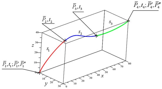
Figure 8. Fifth-degree Hermite spline curve of three segments.

Algorithm 1 For obtaining a spline curve with polynomial equations of the fifth degree of segments $s_1$ and $s_2$ has the following text form:

Vector derivatives ${\overline{P}}_2^{\prime }$ and ${\overline{P}}_2^{″}$ at the joining point ${\overline{P}}_2$ of segments $s_1$ and $s_2$ are determined based on the Formulas (9) and (10). Determine the vector coefficients ${\overline{A}}_i^{(1)}$ in the segment equation $s_1$ based on the matrix (2). In this case, the boundary conditions of the segment $s_1$ are the given vector derivatives ${\overline{P}}_1^{\prime }$ and ${\overline{P}}_1^{″}$ at the knot ${\overline{P}}_1$ and the vector derivatives ${\overline{P}}_2^{\prime }$ and ${\overline{P}}_2^{″}$ at the knot ${\overline{P}}_2$ determined according to item 1. Determine the vector coefficients ${\overline{A}}_i^{(2)}$ in the segment equation $s_2$ based on matrix (2). In this case, the boundary conditions of the segment $s_2$ are the vector derivatives ${\overline{P}}_2^{\prime }$ and ${\overline{P}}_2^{″}$ at the knot ${\overline{P}}_2$ determined according to item 1 and the given vector derivatives ${\overline{P}}_3^{\prime }$ and ${\overline{P}}_3^{″}$ at the knot ${\overline{P}}_3$.

The values of curvature and torsion at boundary points ${\overline{P}}_j$, $j=1,\dots ,4$ of the connected segments are listed in Table 1.

Table 1. Curvature and torsion values at boundary points of the segments.

Segment	Segment Boundary Knot Point ${\overline{\mathit{P}}}_{\mathit{j}}$	Curvature Value	Torsion Value
$s_1:{\overline{p}}_1(t)$	${\overline{P}}_1$, t = 0	3.941914854	−0.5087014266
	${\overline{P}}_2$, t = 1	0.02817282676	−0.002966524102
$s_2:{\overline{p}}_2(t)$	${\overline{P}}_2$, t = 0	0.02817282676	−0.002966524102
	${\overline{P}}_3$, t = 1	0.02036895463	0.006197310968
$s_3:{\overline{p}}_3(t)$	${\overline{P}}_3$, t = 0	0.02036895463	0.006197310968
	${\overline{P}}_4$, t = 1	5.641693337	7.620878085

Example 2.

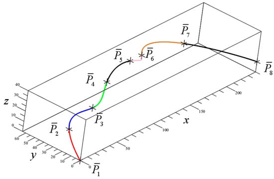
Figure 9 and Table 2 show the result of construction of a fifth-degree Hermite spline curve consisting of seven segments given the following knot points and boundary conditions:${\overline{P}}_1(0,0,0)$,${\overline{P}}_2(20,30,10)$,${\overline{P}}_3(50,30,20)$,${\overline{P}}_4(80,40,30)$,${\overline{P}}_5(110,40,40)$,${\overline{P}}_6(140,50,30)$,${\overline{P}}_7(200,50,20)$,${\overline{P}}_8(240,0,10)$,${\overline{P}}_1^{\prime }(1,3,1)$,${\overline{P}}_8^{\prime }(0,1,-1)$,${\overline{P}}_1^{″}(-1,1,2)$,${\overline{P}}_8^{″}(0,2,1)$. The method and the algorithm are identical to the ones applied in Example 1.

Figure 9. Fifth-degree Hermite spline curve of seven segments.

Table 2. Curvature and torsion values at boundary points of the segments.

Segment	Segment Boundary Knot Point ${\overline{\mathit{P}}}_{\mathit{j}}$	Curvature Value	Torsion Value
$s_1:{\overline{p}}_1(t)$	${\overline{P}}_1$, t = 0	0.1938188331	5.856231764
	${\overline{P}}_2$, t = 1	0.02278819120	0.000690202
$s_2:{\overline{p}}_2(t)$	${\overline{P}}_2$, t = 0	0.02278819120	0.000690202
	${\overline{P}}_3$, t = 1	0.04837483783	0.019236811
…	…	…	…
$s_6:{\overline{p}}_6(t)$	${\overline{P}}_6$, t = 0	0.00690588217	0.182303253
	${\overline{P}}_7$, t = 1	0.01015952078	0.001620745
$s_7:{\overline{p}}_7(t)$	${\overline{P}}_7$, t = 0	0.01015952078	0.001620745
	${\overline{P}}_8$, t = 1	1.060660172	215.2425767

The solution of the examples 1 and 2 allow us to generalize the proposed algorithm and solution method for the case of $(j-1)$ connected segments of fifth-degree Hermite spline curve.

The system of linear equations for the case of unknown ${\overline{P}}_2^{\prime },{\overline{P}}_3^{\prime },\dots ,{\overline{P}}_{j-2}^{\prime },{\overline{P}}_{j-1}^{\prime }$ and ${\overline{P}}_2^{″},{\overline{P}}_3^{″},\dots ,{\overline{P}}_{j-2}^{″},{\overline{P}}_{j-1}^{″}$ is of the following form

$$\{\begin{array}{l}16{\overline{P}}_2^{\prime }+7{\overline{P}}_3^{\prime }-{\overline{P}}_3^{″}=-15({\overline{P}}_1-{\overline{P}}_3)-7{\overline{P}}_1^{\prime }-{\overline{P}}_1^{″},\\ -4{\overline{P}}_3^{\prime }-3{\overline{P}}_2^{″}+\frac{1}{2}{\overline{P}}_3^{″}=-10({\overline{P}}_1-2{\overline{P}}_2+{\overline{P}}_3)+4{\overline{P}}_1^{\prime }+\frac{1}{2}{\overline{P}}_1^{″},\\ 7{\overline{P}}_2^{\prime }+16{\overline{P}}_3^{\prime }+7{\overline{P}}_4^{\prime }+{\overline{P}}_2^{″}-{\overline{P}}_4^{″}=-15({\overline{P}}_2-{\overline{P}}_4),\\ 4{\overline{P}}_3^{\prime }-4{\overline{P}}_4^{\prime }+\frac{1}{2}{\overline{P}}_2^{″}-3{\overline{P}}_3^{″}+\frac{1}{2}{\overline{P}}_4^{″}=-10({\overline{P}}_2-2{\overline{P}}_3+{\overline{P}}_4),\\ \dots \dots \dots \dots \dots \dots \dots \dots \dots \dots \dots \dots \dots \dots \dots \dots \dots \dots \dots \\ 7{\overline{P}}_{j-2}^{\prime }+16{\overline{P}}_{j-1}^{\prime }+{\overline{P}}_{j-2}^{\prime }=-15({\overline{P}}_{j-2}-{\overline{P}}_j)-7{\overline{P}}_j^{\prime }+{\overline{P}}_j^{″},\\ 4{\overline{P}}_{j-1}^{\prime }+\frac{1}{2}{\overline{P}}_{j-2}^{\prime }-3{\overline{P}}_{j-1}^{″}=-10({\overline{P}}_{j-2}-2{\overline{P}}_{j-1}+{\overline{P}}_j)-4{\overline{P}}_j^{\prime }+\frac{1}{2}{\overline{P}}_j^{″}.\end{array}.$$

(13)

The generalized system of Equation (13) can be expressed in the following matrix form

$$\begin{array}{ccccccccccccccccc}& {\overline{P}}_2^{\prime }& {\overline{P}}_3^{\prime }& {\overline{P}}_4^{\prime }& \dots & {\overline{P}}_{j-2}^{\prime }& {\overline{P}}_{j-1}^{\prime }& & & {\overline{P}}_2^{″}& {\overline{P}}_3^{″}& {\overline{P}}_4^{″}& \dots & {\overline{P}}_{j-2}^{″}& {\overline{P}}_{j-1}^{″}& & \\ & 16& 7& 0& \dots & 0& 0& & & 0& -1& 0& \dots & 0& 0& & -15({\overline{P}}_1-{\overline{P}}_3)-7{\overline{P}}_1^{\prime }-{\overline{P}}_1^{″}\\ & 0& -4& 0& \dots & 0& 0& & & -3& \frac{1}{2}& 0& \dots & 0& 0& & -10({\overline{P}}_1-2{\overline{P}}_2+{\overline{P}}_3)+4{\overline{P}}_1^{\prime }+\frac{1}{2}{\overline{P}}_1^{″}\\ & 7& 16& 7& \dots & 0& 0& & & 1& 0& -1& \dots & 0& 0& & -15({\overline{P}}_2-{\overline{P}}_4)\\ & 0& 4& -4& \dots & 0& 0& & & \frac{1}{2}& -3& \frac{1}{2}& \dots & 0& 0& & -10({\overline{P}}_2-2{\overline{P}}_3+{\overline{P}}_4)\\ & \dots & \dots & \dots & \dots & \dots & \dots & & & \dots & \dots & \dots & \dots & \dots & \dots & & \dots \\ & 0& 0& 0& 0& 7& 16& & & 0& 0& 0& \dots & 1& 0& & -15({\overline{P}}_{j-2}-{\overline{P}}_j)-7{\overline{P}}_j^{\prime }+{\overline{P}}_j^{″}\\ & 0& 0& 0& 0& 0& 4& & & 0& 0& 0& \dots & \frac{1}{2}& -3& & -10({\overline{P}}_{j-2}-2{\overline{P}}_{j-1}+{\overline{P}}_j)-4{\overline{P}}_j^{\prime }+\frac{1}{2}{\overline{P}}_j^{″}\end{array}$$

(14)

The generalized system matrix (parametric matrix) (13) or (14) consists of $2(j-2)$ linear equations in $2(j-2)$ unknown. It is of size $2(j-2)\times 2(j-2)$ and holds real numbers. This matrix is invertible and therefore the system of linear equations is uniquely solvable. It can be solved through Gauss–Jordan method, just as the Example above. The matrix Formula (14) of the generalized system of Equation (13) conforms to this method.

3.3. Construction of a Closed Fifth-Degree Hermite Spline Curve

In order to construct a closed Hermite spline curve of i segments subsequently connected in the given j knot points with smoothness $C^4$, it is required to fulfill the following boundary conditions at connection points: ${\overline{P}}_1^{\prime }={\overline{p}}_1^{\prime }(t=0)$, ${\overline{P}}_1^{″}={\overline{p}}_1^{″}(t=0)$, ${\overline{P}}_1^{\prime }={\overline{p}}_j^{\prime }(t=1)$, ${\overline{P}}_1^{″}={\overline{p}}_j^{″}(t=1)$. Taking these conditions into account the matrix (15) is used to determine the vector coefficients of the segment equations.

Example 3.

It is required to construct a closed Hermite spline curve of four segments subsequently connected with smoothness$C^4$at knot points${\overline{P}}_1(0,0,0)$,${\overline{P}}_2(0,100,10)$,${\overline{P}}_3(100,100,20)$,${\overline{P}}_4(100,0,30)$.

Let us add vectors ${\overline{P}}_1^{\prime },{\overline{P}}_1^{″}$ and ${\overline{P}}_4^{\prime },{\overline{P}}_4^{″}$ to the list of unknown vectors in the system of equations and acquire the system of eight equations in eight unknowns:

$$\{\begin{array}{l}7{\overline{P}}_1^{\prime }+16{\overline{P}}_2^{\prime }+7{\overline{P}}_3^{\prime }+{\overline{P}}_1^{″}-{\overline{P}}_3^{″}=-15({\overline{P}}_1-{\overline{P}}_3),\\ 4{\overline{P}}_1^{\prime }-4{\overline{P}}_3^{\prime }+\frac{1}{2}{\overline{P}}_1^{″}-3{\overline{P}}_2^{″}+\frac{1}{2}{\overline{P}}_3^{″}=-10({\overline{P}}_1-2{\overline{P}}_2+{\overline{P}}_3),\\ 7{\overline{P}}_2^{\prime }+16{\overline{P}}_3^{\prime }+7{\overline{P}}_4^{\prime }+{\overline{P}}_2^{″}-{\overline{P}}_4^{″}=-15({\overline{P}}_2-{\overline{P}}_4),\\ 4{\overline{P}}_2^{\prime }-4{\overline{P}}_4^{\prime }+\frac{1}{2}{\overline{P}}_2^{″}-3{\overline{P}}_3^{″}+\frac{1}{2}{\overline{P}}_4^{″}=-10({\overline{P}}_2-2{\overline{P}}_3+{\overline{P}}_4),\\ 7{\overline{P}}_1^{\prime }+7{\overline{P}}_3^{\prime }+16{\overline{P}}_4^{\prime }-{\overline{P}}_1^{″}+{\overline{P}}_3^{″}=-15({\overline{P}}_3-{\overline{P}}_1),\\ -4{\overline{P}}_1^{\prime }+4{\overline{P}}_3^{\prime }+\frac{1}{2}{\overline{P}}_1^{″}+\frac{1}{2}{\overline{P}}_3^{″}-3{\overline{P}}_4^{″}=-10({\overline{P}}_3-2{\overline{P}}_4+{\overline{P}}_1),\\ 16{\overline{P}}_1^{\prime }+7{\overline{P}}_2^{\prime }+7{\overline{P}}_4^{\prime }-{\overline{P}}_2^{″}+{\overline{P}}_4^{″}=-15({\overline{P}}_4-{\overline{P}}_2),\\ -4{\overline{P}}_2^{\prime }+4{\overline{P}}_4^{\prime }-3{\overline{P}}_1^{″}+\frac{1}{2}{\overline{P}}_2^{″}+\frac{1}{2}{\overline{P}}_4^{″}=-10({\overline{P}}_4-2{\overline{P}}_1+{\overline{P}}_2).\end{array}.$$

(15)

Let us transform the system (15) into matrix form in order to facilitate the solution through Gauss–Jordan method (16).

The unknown vector coefficients ${\overline{A}}_i^{(k)},k=1,\dots ,4;i=1,\dots ,6$ are calculated through (16) taking into account the closure. In the case of a closed spline, the matrix for calculating vector coefficients ${\overline{A}}_i^{(k)}$ is expanded by adding a closing segment, the equation of which contains vector coefficients ${\overline{A}}_i^{(k)},i=1,\dots ,6$. Figure 10 and Table 3 show the result of construction of a closed spline curve of four segments.

$$\begin{array}{ccccccccc}{\overline{P}}_1^{\prime }& {\overline{P}}_2^{\prime }& {\overline{P}}_3^{\prime }& {\overline{P}}_4^{\prime }& {\overline{P}}_1^{″}& {\overline{P}}_2^{″}& {\overline{P}}_3^{″}& {\overline{P}}_4^{″}& \\ 7& 16& 7& 0& 1& 0& -1& 0& -15({\overline{P}}_1-{\overline{P}}_3)\\ 4& 0& -4& 0& \frac{1}{2}& -3& \frac{1}{2}& 0& -10(k_5{\overline{P}}_1-2k_6{\overline{P}}_2+{\overline{P}}_3)\\ 0& 7& 16& 7& 0& 1& 0& -1& -15({\overline{P}}_2-{\overline{P}}_4)\\ 0& 4& 0& -4& 0& \frac{1}{2}& -3& \frac{1}{2}& -10({\overline{P}}_2-2{\overline{P}}_3+{\overline{P}}_4)\\ 7& 0& 7& 16& -1& 0& 1& 0& -15({\overline{P}}_3-{\overline{P}}_1)\\ -4& 0& 4& 0& \frac{1}{2}& 0& \frac{1}{2}& -3& -10({\overline{P}}_3-2{\overline{P}}_4+{\overline{P}}_1)\\ 16& 7& 0& 7& 0& -1& 0& 1& -15({\overline{P}}_4-{\overline{P}}_2)\\ 0& -4& 0& 4& -3& \frac{1}{2}& 0& \frac{1}{2}& -10({\overline{P}}_4-2{\overline{P}}_1+{\overline{P}}_2)\end{array}.$$

(16)

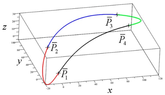
Figure 10. Closed fifth-degree Hermite spline curve of four segments.

Table 3. Curvature and torsion values at boundary points of the segments.

Segment	Segment Boundary Knot Point ${\overline{\mathit{P}}}_{\mathit{j}}$	Curvature Value	Torsion Value
$s_1:{\overline{p}}_1(t)$	${\overline{P}}_1$, t = 0	0.001781606146	0.2447808764
	${\overline{P}}_2$, t = 1	0.005681042934	−0.001318648614
$s_2:{\overline{p}}_2(t)$	${\overline{P}}_2$, t = 0	0.005681042934	−0.001318648614
	${\overline{P}}_3$, t = 1	0.02148171241	−0.005905294855
$s_3:{\overline{p}}_3(t)$	${\overline{P}}_3$, t = 0	0.02148171241	−0.005905294855
	${\overline{P}}_4$, t = 1	0.01654790405	0.02790910517
$s_4:{\overline{p}}_4(t)$	${\overline{P}}_4$, t = 0	0.01654790405	0.02790910517
	${\overline{P}}_5$, t = 1	0.001781606146	0.2447808764

The system of Equation (15) and the matrix Formula (16) can be generalized for the case of j knot points and j segments of a closed Hermite spline curve. The generalized system of equations is of the following matrix form:

$$\begin{array}{ccccccccccccccccc}{\overline{P}}_1^{\prime }& {\overline{P}}_2^{\prime }& {\overline{P}}_3^{\prime }& {\overline{P}}_4^{\prime }& \dots & {\overline{P}}_{j-2}^{\prime }& {\overline{P}}_{j-1}^{\prime }& {\overline{P}}_j^{\prime }& {\overline{P}}_1^{″}& {\overline{P}}_2^{″}& {\overline{P}}_3^{″}& {\overline{P}}_4^{″}& \dots & {\overline{P}}_{j-2}^{″}& {\overline{P}}_{j-1}^{″}& {\overline{P}}_j^{″}& \\ 7& 16& 7& 0& \dots & 0& 0& 0& 1& 0& -1& 0& \dots & 0& 0& 0& -15({\overline{P}}_1-{\overline{P}}_3)\\ 4& 0& -4& 0& \dots & 0& 0& 0& \frac{1}{2}& -3& \frac{1}{2}& 0& \dots & 0& 0& 0& -10({\overline{P}}_1-2{\overline{P}}_2+{\overline{P}}_3)\\ 0& 7& 16& 7& \dots & 0& 0& 0& 0& 1& 0& -1& \dots & 0& 0& 0& -15({\overline{P}}_2-{\overline{P}}_4)\\ 0& 4& 0& -4& \dots & 0& 0& 0& 0& \frac{1}{2}& -3& \frac{1}{2}& \dots & 0& 0& 0& -10({\overline{P}}_2-2{\overline{P}}_3+{\overline{P}}_4)\\ \dots & \dots & \dots & \dots & \dots & \dots & \dots & \dots & \dots & \dots & \dots & \dots & \dots & \dots & \dots & \dots & \dots \\ 0& 0& 0& 0& \dots & 7& 16& 7& 0& 0& 0& 0& \dots & 1& 0& -1& -15({\overline{P}}_{j-2}-{\overline{P}}_j)\\ 0& 0& 0& 0& \dots & 4& 0& -4& 0& 0& 0& 0& \dots & \frac{1}{2}& -3& \frac{1}{2}& -10({\overline{P}}_{j-2}-2{\overline{P}}_{j-1}+{\overline{P}}_j)\\ 7& 0& 0& 0& \dots & 0& 7& 16& -1& 0& 0& 0& \dots & 0& 1& 0& -15({\overline{P}}_{j-1}-{\overline{P}}_1)\\ -4& 0& 0& 0& \dots & 0& 4& 0& \frac{1}{2}& 0& 0& 0& \dots & 0& \frac{1}{2}& -3& -10({\overline{P}}_{j-1}-2{\overline{P}}_j+{\overline{P}}_1)\\ 16& 7& 0& 0& \dots & 0& 0& 7& 0& -1& 0& 0& \dots & 0& 0& 1& -15({\overline{P}}_j-{\overline{P}}_2)\\ 0& -4& 0& 0& \dots & 0& 0& 4& -3& \frac{1}{2}& 0& 0& \dots & 0& 0& \frac{1}{2}& -10({\overline{P}}_j-2{\overline{P}}_1+{\overline{P}}_2)\end{array}$$

(17)

The matrix of generalized system of equations consists of $2j$ linear equations in $2j$ unknown ${\overline{P}}_1^{\prime },{\overline{P}}_2^{\prime },\dots {\overline{P}}_{j-1}^{\prime },{\overline{P}}_j^{\prime }$; ${\overline{P}}_1^{″},{\overline{P}}_2^{″},\dots {\overline{P}}_{j-1}^{″},{\overline{P}}_j^{″}$ and is of size $2j\times 2j$. Its elements are also real numbers. It is invertible and therefore the system of linear equations is uniquely solvable. It can also be solved through the Gauss–Jordan method. The matrix Formula (17) conforms to this method.

Example 4.

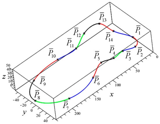
Figure 11 and Table 4 show the results of construction of a closed Hermite spline curve of 14 segments given the knot points:${\overline{P}}_1(0,0,0)$,${\overline{P}}_2(20,30,10)$,${\overline{P}}_3(50,30,20)$,${\overline{P}}_4(80,40,30)$,${\overline{P}}_5(110,40,40)$,${\overline{P}}_6(140,50,30)$,${\overline{P}}_7(200,50,20)$,${\overline{P}}_8(240,0,10)$,${\overline{P}}_9(200,-50,0)$,${\overline{P}}_{10}(140,-50,10)$,${\overline{P}}_{11}(110,-30,30)$,${\overline{P}}_{12}(80,-40,40)$,${\overline{P}}_{13}(50,-30,50)$,${\overline{P}}_{14}(20,-30,10)$. The method and the algorithm are identical to the ones applied in Example 3.

Figure 11. Closed fifth-degree Hermite spline curve of 14 segments.

Table 4. Curvature and torsion values at boundary points of the segments.

Segment	Segment Boundary Knot Point ${\overline{\mathit{P}}}_{\mathit{j}}$	Curvature Value	Torsion Value
$s_1:{\overline{p}}_1(t)$	${\overline{P}}_1$, t = 0	0.02804073313	0.01755939453
	${\overline{P}}_2$, t = 1	0.03647568313	−0.009461103708
$s_2:{\overline{p}}_2(t)$	${\overline{P}}_2$, t = 0	0.03647568313	−0.009461103708
	${\overline{P}}_3$, t = 1	0.02872143869	0.006884363759
…	…	…	…
$s_{13}:{\overline{p}}_{13}(t)$	${\overline{P}}_{13}$, t = 0	0.06756281437	0.008605623218
	${\overline{P}}_{13}$, t = 1	0.02578660580	0.005023460581
$s_{14}:{\overline{p}}_{14}(t)$	${\overline{P}}_{14}$, t = 0	0.02578660580	0.005023460581
	${\overline{P}}_{14}$, t = 1	0.02804073313	0.01755939453

3.4. Construction of a Hermite Segment Given Boundary Derivatives of First, Second, and Third Orders

Given points ${\overline{P}}_1(x_1,y_1,z_1)$ and ${\overline{P}}_2(x_2,y_2,z_2)$ with the respective boundary conditions ${\overline{P}}_1^{\prime }$, ${\overline{P}}_1^{″}$, ${\overline{P}}_1^{‴}$ and ${\overline{P}}_2^{\prime }$, ${\overline{P}}_2^{″}$, ${\overline{P}}_2^{‴}$(see Figure 12), it is required to construct a segment of a Hermite spline curve.

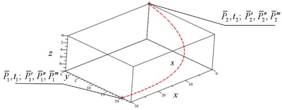
Figure 12. Initial conditions for construction of a seventh-degree Hermite spline curve segment.

Obviously, a segment of Hermite spline curve has to be described by a polynomial

$$\overline{p}(t)={\displaystyle \sum _{i=1}^8{\overline{A}}_i}{t}^{i-1},t_1\le t\le t_2.$$

(18)

Vectors ${\overline{P}}_1^{\prime }$, ${\overline{P}}_2^{\prime }$ are the first vector derivatives constituting tangent vectors at the endpoints of the sought segment s. ${\overline{P}}_1^{″},{\overline{P}}_2^{″}$ are the second vector derivatives constituting vectors of acceleration of a point tracing out the segment s and ${\overline{P}}_1^{‴},{\overline{P}}_2^{‴}$ are the third vector derivatives constituting vectors of jerk of a point tracing out the segment s. Obviously, the given conditions are sufficient in order to define the vector coefficients ${\overline{A}}_i$ of the Formula (18). Let us express the first, the second, and the third derivatives of vector function $\overline{p}(t)$

$$\begin{array}{c}{\overline{p}}^{\prime }(t)={\displaystyle \sum _{i=2}^8{\overline{A}}_i(i-1)}{t}^{i-2},{\overline{p}}^{″}(t)={\displaystyle \sum _{i=3}^8{\overline{A}}_i(i-1)(i-2)}{t}^{i-3},\\ {\overline{p}}^{‴}(t)={\displaystyle \sum _{i=4}^8{\overline{A}}_i(i-1)(i-2)(i-3)}{t}^{i-4}.\end{array}$$

We apply parameterization $0\le t\le 1$. In this case the values of the first four vector coefficients can be acquired

$$\begin{array}{c}\overline{p}(0)={\overline{P}}_1={\overline{A}}_1;{\overline{p}}^{\prime }(0)={\overline{P}}_1^{\prime }={\overline{A}}_2;{\overline{p}}^{″}(0)={\overline{P}}_1^{″}=2{\overline{A}}_3,\mathrm{i}.\mathrm{e}.{\overline{A}}_3=\frac{1}{2}{\overline{P}}_1^{″};\\ {\overline{p}}^{‴}(0)={\overline{P}}_1^{‴}=6{\overline{A}}_4,\mathrm{i}.\mathrm{e}.{\overline{A}}_4=\frac{1}{6}{\overline{P}}_1^{‴}.\end{array}$$

(19)

The rest of the vector coefficients are determined through the equations

$$\overline{p}(t_2)={\overline{P}}_2,{\overline{p}}^{\prime }(t_2)={\overline{P}}_2^{\prime },{\overline{p}}^{″}(t_2)={\overline{P}}_2^{″},{\overline{p}}^{‴}(t_2)={\overline{P}}_2^{‴},$$

that lead us to the system of four linear equations

$$\{\begin{array}{l}{\displaystyle \sum _{i=1}^8{\overline{A}}_i}{t}_2^{i-1}-{\overline{P}}_2=0,\\ {\displaystyle \sum _{i=2}^8{\overline{A}}_i(i-1)}{t}_2^{i-2}-{\overline{P}}_2^{\prime }=0,\\ {\displaystyle \sum _{i=3}^8{\overline{A}}_i(i-1)(i-2)}{t}_2^{i-3}-{\overline{P}}_2^{″}=0,\\ {\displaystyle \sum _{i=4}^8{\overline{A}}_i(i-1)(i-2)(i-3)}{t}_2^{i-4}-{\overline{P}}_2^{‴}=0.\end{array}$$

(20)

The values of coefficients ${\overline{A}}_5,{\overline{A}}_6,{\overline{A}}_7$ and ${\overline{A}}_8$ follow from the system of Equation (20)

$${\overline{A}}_5=-35{\overline{P}}_1+35{\overline{P}}_2-20{\overline{P}}_1^{\prime }-15{\overline{P}}_2^{\prime }-5{\overline{P}}_1^{″}+\frac{5}{2}{\overline{P}}_2^{″}-\frac{2}{3}{\overline{P}}_1^{‴}-\frac{1}{2}{\overline{P}}_2^{‴},$$

$${\overline{A}}_6=84{\overline{P}}_1-84{\overline{P}}_2+45{\overline{P}}_1^{\prime }+39{\overline{P}}_2^{\prime }+10{\overline{P}}_1^{″}-7{\overline{P}}_2^{″}+{\overline{P}}_1^{‴}+\frac{1}{2}{\overline{P}}_2^{‴},$$

$${\overline{A}}_7=-70{\overline{P}}_1+70{\overline{P}}_2-36{\overline{P}}_1^{\prime }-34{\overline{P}}_2^{\prime }-\frac{15}{2}{\overline{P}}_1^{″}+\frac{13}{2}{\overline{P}}_2^{″}-\frac{2}{3}{\overline{P}}_1^{‴}-\frac{1}{2}{\overline{P}}_2^{‴},$$

$${\overline{A}}_8=20({\overline{P}}_1-{\overline{P}}_2)+10({\overline{P}}_1^{\prime }+{\overline{P}}_2^{\prime })+2({\overline{P}}_1^{″}-{\overline{P}}_2^{″})+\frac{1}{6}({\overline{P}}_1^{‴}+{\overline{P}}_2^{‴}).$$

Let us transform the expressions (19) and (20) into the matrix form

$$\left[\overline{A}\right]=\left[\begin{array}{c}{\overline{A}}_1\\ {\overline{A}}_2\\ {\overline{A}}_3\\ {\overline{A}}_4\\ {\overline{A}}_5\\ \begin{array}{l}{\overline{A}}_6\\ {\overline{A}}_7\\ {\overline{A}}_8\end{array}\end{array}\right]=\left[\begin{array}{cccccccc}1& 0& 0& 0& 0& 0& 0& 0\\ 0& 0& 1& 0& 0& 0& 0& 0\\ 0& 0& 0& 0& 0.5& 0& 0& 0\\ 0& 0& 0& 0& 0& 0& \frac{1}{6}& 0\\ -35& 35& -20& -15& -5& \frac{5}{2}& -\frac{2}{3}& -\frac{1}{2}\\ 84& -84& 45& 39& 10& -7& 1& \frac{1}{2}\\ -70& 70& -36& -34& -\frac{15}{2}& \frac{13}{2}& -\frac{2}{3}& -\frac{1}{2}\\ 20& -20& 10& 10& 2& -2& \frac{1}{6}& \frac{1}{6}\end{array}\right]\cdot \left[\begin{array}{c}{\overline{P}}_1\\ {\overline{P}}_2\\ \begin{array}{l}{\overline{P}}_1^{\prime }\\ {\overline{P}}_2^{\prime }\end{array}\\ {\overline{P}}_1^{″}\\ \begin{array}{l}{\overline{P}}_2^{″}\\ {\overline{P}}_1^{‴}\end{array}\\ {\overline{P}}_2^{‴}\end{array}\right].$$

(21)

If we substitute the expressions of vector coefficients (21) into the Formula (18), we acquire the sought equation of a Hermite spline curve segment.

3.5. Construction of a Seventh-Degree Hermite Spline Curve of Two Segments and Generalization for the Case of (j − 1) Segments

Let us consider connection of two segments $s_1$ and $s_2$ (see Figure 13) given the same boundary conditions as for the case of one segment s previously considered in Section 3.4. Parameterization of segments is fulfilled in ranges $t_1\le t\le t_2$ and $t_2\le t\le t_3$ for respective segments $s_1$ and $s_2$. Without loss of generality, we accept that $t_1=0$ at the initial point of segment $s_1$ and $t_2=0$ at the initial point of segment $s_2$. Let us express the polynomial equation of the segments in the following form: ${\overline{p}}_k(t)={\displaystyle \sum _{i=1}^8{\overline{A}}_i^{(k)}}{t}^{i-1};k=1,2$. Let us express the derivatives of vector function ${\overline{p}}_k(t)$

$$\begin{array}{c}{\overline{p}}_k^{\prime }(t)={\displaystyle \sum _{i=2}^8{\overline{A}}_i^{(k)}(i-1)}{t}^{i-2},{\overline{p}}_k^{″}(t)={\displaystyle \sum _{i=3}^8{\overline{A}}_i^{(k)}(i-1)(i-2)}{t}^{i-3},\\ {\overline{p}}_k^{‴}(t)={\displaystyle \sum _{i=4}^8{\overline{A}}^{(k)}{}_i(i-1)(i-2)(i-3)}{t}^{i-4}.\end{array}$$

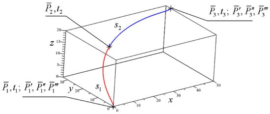
Figure 13. Seventh-degree Hermite spline curve of two segments.

For k =1 at the initial point ${\overline{P}}_1(t_1=0)$ of segment $s_1$ we acquire

$${\overline{p}}_1(0)={\overline{P}}_1={\overline{A}}_1^{(1)},{\overline{p}}_1^{\prime }(0)={\overline{P}}_1^{\prime }={\overline{A}}_2^{(1)},{\overline{p}}_1^{″}(0)={\overline{P}}_1^{″}=2{\overline{A}}_3^{(1)},{\overline{p}}_1^{‴}(0)={\overline{P}}_1^{‴}=6{\overline{A}}_4^{(1)}.$$

(22)

At the final point ${\overline{P}}_2(t_2)$ of segment $s_1$ we acquire

$$\begin{array}{c}{\overline{p}}_1(t_2)={\overline{P}}_2={\displaystyle \sum _{i=1}^8{\overline{A}}_i^{(1)}}{t}_2^{i-1},{\overline{p}}_1^{\prime }(t_2)={\overline{P}}_2^{\prime }={\displaystyle \sum _{i=2}^8{\overline{A}}_i^{(1)}(i-1)}{t}_2^{i-2},{\overline{p}}_1^{″}(t_2)={\overline{P}}_2^{″}={\displaystyle \sum _{i=3}^6{\overline{A}}_i^{(1)}(i-1)(i-2)}{t}_2^{i-3},\\ {\overline{p}}_1^{‴}(t_2)={\displaystyle \sum _{i=4}^8{\overline{A}}^{(1)}{}_i(i-1)(i-2)(i-3)}{t}_2^{i-4}.\end{array}$$

For k = 2 at the initial point ${\overline{P}}_2(t_2=0)$ of segment $s_2$ we acquire

$${\overline{p}}_2(0)={\overline{P}}_2={\overline{A}}_1^{(2)},{\overline{p}}_2^{\prime }(0)={\overline{P}}_2^{\prime }={\overline{A}}_2^{(2)},{\overline{p}}_2^{″}(0)={\overline{P}}_2^{″}=2{\overline{A}}_3^{(2)},{\overline{p}}_2^{‴}(0)={\overline{P}}_2^{‴}=6{\overline{A}}_4^2.$$

(23)

At the final point ${\overline{P}}_3(t_3)$ of segment $s_2$ we acquire

$$\begin{array}{c}{\overline{p}}_2(t_3)={\overline{P}}_3={\displaystyle \sum _{i=1}^8{\overline{A}}_i^{(2)}}{t}_3^{i-1},{\overline{p}}_2^{\prime }(t_3)={\overline{P}}_3^{\prime }={\displaystyle \sum _{i=2}^8{\overline{A}}_i^{(2)}(i-1)}{t}_3^{i-2},{\overline{p}}_2^{″}(t_3)={\overline{P}}_3^{″}={\displaystyle \sum _{i=3}^8{\overline{A}}_i^{(2)}(i-1)(i-2)}{t}_3^{i-3},\\ {\overline{p}}_2^{‴}(t_3)={\displaystyle \sum _{i=4}^8{\overline{A}}^{(2)}{}_i(i-1)(i-2)(i-3)}{t}_3^{i-4}.\end{array}$$

Thus, through (22), we acquire the expressions for the first four coefficients of the equation for the first segment $s_1$: ${\overline{A}}_1^{(1)}={\overline{P}}_1,{\overline{A}}_2^{(1)}={\overline{P}}_1^{\prime },{\overline{A}}_3^{(1)}=\frac{1}{2}{\overline{P}}_1^{″},$ ${\overline{A}}_4^{(1)}=\frac{1}{6}{\overline{P}}_1^{″}$. The remaining vector coefficients ${\overline{A}}_5^{(1)},{\overline{A}}_6^{(1)},{\overline{A}}_7^{(1)},{\overline{A}}_8^{(1)}$ are determined through the system of four linear equations

$$\{\begin{array}{l}{\displaystyle \sum _{i=1}^8{\overline{A}}_i^{(1)}}{t}_2^{i-1}-{\overline{P}}_2=0,\\ {\displaystyle \sum _{i=2}^8{\overline{A}}_i^{(1)}(i-1)}{t}_2^{i-2}-{\overline{P}}_2^{\prime }=0,\\ {\displaystyle \sum _{i=3}^8{\overline{A}}_i^{(1)}(i-1)(i-2)}{t}_2^{i-3}-{\overline{P}}_2^{″}=0,\\ {\displaystyle \sum _{i=4}^8{\overline{A}}^{(1)}{}_i(i-1)(i-2)(i-3)}{t}_2^{i-4}-{\overline{P}}_2^{‴}.\end{array}$$

(24)

The expressions of the first four vector coefficients of segment $s_2$ follow from (23): ${\overline{A}}_1^{(2)}={\overline{P}}_2,{\overline{A}}_2^{(2)}={\overline{P}}_2^{\prime },{\overline{A}}_3^{(2)}=\frac{1}{2}{\overline{P}}_2^{″},{\overline{A}}_4^{(2)}=\frac{1}{6}{\overline{P}}_2^{‴}$. The remaining vector coefficients ${\overline{A}}_5^{(2)}$, ${\overline{A}}_6^{(2)}$, ${\overline{A}}_7^{(2)}$, and ${\overline{A}}_8^{(2)}$ are determined through the system of four linear equations

$$\{\begin{array}{l}{\displaystyle \sum _{i=1}^8{\overline{A}}_i^{(2)}}{t}_3^{i-1}-{\overline{P}}_3=0,\\ {\displaystyle \sum _{i=2}^8{\overline{A}}_i^{(2)}(i-1)}{t}_3^{i-2}-{\overline{P}}_3^{\prime }=0,\\ {\displaystyle \sum _{i=3}^8{\overline{A}}_i^{(2)}(i-1)(i-2)}{t}_3^{i-3}-{\overline{P}}_3^{″}=0,\\ {\displaystyle \sum _{i=4}^8{\overline{A}}^{(2)}{}_i(i-1)(i-2)(i-3)}{t}_3^{i-4}-{\overline{P}}_3^{‴}.\end{array}$$

(25)

Vectors ${\overline{P}}_2^{\prime }$, ${\overline{P}}_2^{″}$, and ${\overline{P}}_2^{‴}$ at the knot ${\overline{P}}_2$ of connection of segments $s_1$ and $s_2$ are unknown. These vectors are determined through the conditions of equality of fourth, fifth, and sixth derivatives of vector functions at the connection knot:

${\overline{p}}_1^{⁗}(t=t_2)={\overline{p}}_2^{⁗}(t=0)$, or in expanded form

$$4{\overline{A}}_5^{(1)}+120{\overline{A}}_6^{(1)}{t}_2+360{\overline{A}}_7^{(1)}{t}_2^2+840{\overline{A}}_8^{(1)}{t}_2^3=24{\overline{A}}_5^{(2)}.$$

(26)

${\overline{p}}_1^{″‴}(t=t_2)={\overline{p}}_2^{″‴}(t=0)$, or in expanded form

$$120{\overline{A}}_6^{(1)}+720{\overline{A}}_7^{(1)}{t}_2+2520{\overline{A}}_8^{(1)}{t}_2^2=120{\overline{A}}_6^{(2)}.$$

(27)

${\overline{p}}_1^{‴‴}(t=t_2)={\overline{p}}_2^{‴‴}(t=0)$, or in expanded form

$$720{\overline{A}}_7^{(1)}+5040{\overline{A}}_8^{(1)}{t}_2=720{\overline{A}}_7^{(2)}.$$

(28)

The sought vectors ${\overline{P}}_2^{\prime }$, ${\overline{P}}_2^{″}$, and ${\overline{P}}_2^{‴}$ are determined through the system of linear Equations (25)–(27) taking into account the Equations (23) and (24) with parameterization $0\le t\le 1$ for segments $s_1$ and $s_2$

$${\overline{P}}_2^{\prime }=-\frac{19}{32}{\overline{P}}_1^{\prime }-\frac{19}{32}{\overline{P}}_3^{\prime }-\frac{1}{8}{\overline{P}}_1^{″}+\frac{1}{8}{\overline{P}}_3^{″}-\frac{1}{96}{\overline{P}}_1^{‴}-\frac{1}{96}{\overline{P}}_3^{‴}-\frac{35}{32}({\overline{P}}_1-{\overline{P}}_3),$$

(29)

$${\overline{P}}_2^{″}=\frac{39}{20}{\overline{P}}_1^{\prime }-\frac{39}{20}{\overline{P}}_3^{\prime }+\frac{7}{20}{\overline{P}}_1^{″}+\frac{7}{20}{\overline{P}}_3^{″}+\frac{1}{40}{\overline{P}}_1^{‴}-\frac{1}{40}{\overline{P}}_3^{‴}+\frac{21}{5}({\overline{P}}_1-2{\overline{P}}_2+{\overline{P}}_3)$$

(30)

$${\overline{P}}_2^{‴}=\frac{105}{16}{\overline{P}}_1^{\prime }+\frac{105}{16}{\overline{P}}_3^{\prime }+\frac{15}{8}{\overline{P}}_1^{″}-\frac{15}{8}{\overline{P}}_3^{″}+\frac{3}{16}{\overline{P}}_1^{‴}+\frac{3}{16}{\overline{P}}_3^{‴}+\frac{105}{16}({\overline{P}}_1-{\overline{P}}_3)$$

(31)

The matrix Formula (21) and Algorithm 2 allow us to generalize to the case of the formation of a smooth spline Hermite curve from (j − 1) segments.

In the generalized representation the matrix of vector coefficients $\left[\overline{A}\right]=\left[T\right]\cdot \left[\overline{G}\right]$ for the equations of $(j-1)$ segments of the Hermitian spline curve of the seventh-degree, connected by the smoothness $C^6$, has the Formula (32).

$$\left[\overline{A}\right]=\left[\begin{array}{l}{\overline{A}}_1^{(1)}\\ {\overline{A}}_2^{(1)}\\ {\overline{A}}_3^{(1)}\\ {\overline{A}}_4^{(1)}\\ {\overline{A}}_5^{(1)}\\ {\overline{A}}_6^{(1)}\\ {\overline{A}}_7^{(1)}\\ {\overline{A}}_8^{(1)}\\ \dots \\ {\overline{A}}_1^{(j-1)}\\ {\overline{A}}_2^{(j-1)}\\ {\overline{A}}_3^{(j-1)}\\ {\overline{A}}_4^{(j-1)}\\ {\overline{A}}_5^{(j-1)}\\ {\overline{A}}_6^{(j-1)}\\ {\overline{A}}_7^{(j-1)}\\ {\overline{A}}_8^{(j-1)}\end{array}\right]=\left[\begin{array}{cccccccccccccccccccc}1& 0& \dots & 0& 0& 0& 0& \dots & 0& 0& 0& 0& \dots & 0& 0& 0& 0& \dots & 0& 0\\ 0& 0& \dots & 0& 0& 1& 0& \dots & 0& 0& 0& 0& \dots & 0& 0& 0& 0& \dots & 0& 0\\ 0& 0& \dots & 0& 0& 0& 0& \dots & 0& 0& \frac{1}{2}& 0& \dots & 0& 0& 0& 0& \dots & 0& 0\\ 0& 0& \dots & 0& 0& 0& 0& \dots & 0& 0& 0& 0& \dots & 0& 0& \frac{1}{6}& 0& \dots & 0& 0\\ -35& 35& \dots & 0& 0& -20& -15& \dots & 0& 0& -5& \frac{5}{2}& \dots & 0& 0& -\frac{3}{2}& -\frac{1}{2}& \dots & 0& 0\\ 84& -84& \dots & 0& 0& 45& 39& \dots & 0& 0& 10& -7& \dots & 0& 0& 1& \frac{1}{2}& \dots & 0& 0\\ -70& 70& \dots & 0& 0& -36& -34& \dots & 0& 0& -\frac{15}{2}& \frac{13}{2}& \dots & 0& 0& -\frac{2}{3}& -\frac{1}{2}& \dots & 0& 0\\ 20& -20& \dots & 0& 0& 10& 10& \dots & 0& 0& 2& -2& \dots & 0& 0& \frac{1}{6}& \frac{1}{6}& \dots & 0& 0\\ \dots & \dots & \dots & \dots & \dots & \dots & \dots & \dots & \dots & \dots & \dots & \dots & \dots & \dots & \dots & \dots & \dots & \dots & \dots & \dots \\ 0& 0& \dots & 1& 0& 0& 0& \dots & 0& 0& 0& 0& \dots & 0& 0& 0& 0& \dots & 0& 0\\ 0& 0& \dots & 0& 0& 0& 0& \dots & 1& 0& 0& 0& \dots & 0& 0& 0& 0& \dots & 0& 0\\ 0& 0& \dots & 0& 0& 0& 0& \dots & 0& 0& 0& 0& \dots & \frac{1}{2}& 0& 0& 0& \dots & 0& 0\\ 0& 0& \dots & 0& 0& 0& 0& \dots & 0& 0& 0& 0& \dots & 0& 0& 0& 0& \dots & \frac{1}{6}& 0\\ 0& 0& \dots & -35& 35& 0& 0& \dots & -20& -15& 0& 0& \dots & -5& \frac{5}{2}& 0& 0& \dots & -\frac{2}{3}& -\frac{1}{2}\\ 0& 0& \dots & 84& -84& 0& 0& \dots & 45& 39& 0& 0& \dots & 10& -7& 0& 0& \dots & 1& \frac{1}{2}\\ 0& 0& \dots & -70& 70& 0& 0& \dots & -36& -34& 0& 0& \dots & -\frac{15}{2}& \frac{13}{2}& 0& 0& \dots & -\frac{2}{3}& -\frac{1}{2}\\ 0& 0& \dots & 20& -20& 0& 0& \dots & 10& 10& 0& 0& \dots & 2& -2& 0& 0& \dots & \frac{1}{6}& \frac{1}{6}\end{array}\right]\cdot \left[\begin{array}{c}{\overline{P}}_1\\ {\overline{P}}_2\\ \dots \\ {\overline{P}}_{j-1}\\ {\overline{P}}_j\\ {\overline{P}}_1^{\prime }\\ {\overline{P}}_2^{\prime }\\ \dots \\ {\overline{P}}_{j-1}^{\prime }\\ {\overline{P}}_j^{\prime }\\ {\overline{P}}_1^{″}\\ {\overline{P}}_2^{″}\\ \dots \\ {\overline{P}}_{j-1}^{″}\\ {\overline{P}}_j^{″}\\ {\overline{P}}_1^{‴}\\ {\overline{P}}_2^{‴}\\ \dots \\ {\overline{P}}_{j-1}^{‴}\\ {\overline{P}}_j^{‴}\end{array}\right].$$

(32)

Example 5.

It is required to construct a Hermite spline curve of the seventh degree consisting of three segments given the following boundary conditions:${\overline{P}}_1(20,0,0)$,${\overline{P}}_2(20,10,10)$,${\overline{P}}_3(50,15,20)$,${\overline{P}}_4(80,0,20)$,${\overline{P}}_1^{\prime }(1,0,-1)$,${\overline{P}}_4^{\prime }(-1,0,2)$,${\overline{P}}_1^{″}(1,1,2)$,${\overline{P}}_4^{″}(-1,-3,0)$,${\overline{P}}_1^{‴}(1,0,1)$,${\overline{P}}_4^{‴}(-1,1,0)$.

In order to construct a spline curve, let us apply the matrix Formula (32) for the case $(j-1)=3$. In this case, the vector parameters of the geometric matrix $\left[\overline{G}\right]$ are determined through a uniquely solvable system of six linear equations in six unknowns.

Figure 14 depicts visual rendering of the result of the calculation. It demonstrates the sought three segments and their subsequent connection with order of smoothness $C^6$.

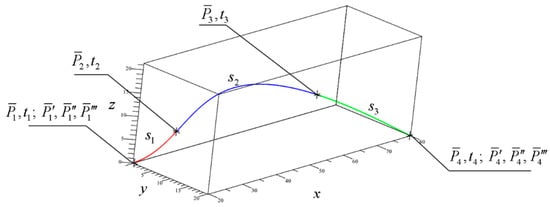
Figure 14. Initial data and the result of connection of three segments of a seventh-degree Hermite spline curve.

Algorithm 2 For obtaining a spline curve with polynomial equations of the seventh degree of segments $s_1$ and $s_2$ has the following text form:

Vector derivatives ${\overline{P}}_2^{\prime }$, ${\overline{P}}_2^{″}$, and ${\overline{P}}_2^{‴}$ at the joining point ${\overline{P}}_2$ of segments $s_1$ and $s_2$ are determined based on the Formulas (29)–(31). Determine the vector coefficients ${\overline{A}}_i^{(1)}$ in the segment equation $s_1$ based on the matrix (20). In this case, the boundary conditions of the segment $s_1$ are the given vector derivatives ${\overline{P}}_1^{\prime }$, ${\overline{P}}_1^{″}$, and ${\overline{P}}_1^{‴}$ at the knot ${\overline{P}}_1$ and the vector derivatives ${\overline{P}}_2^{\prime }$, ${\overline{P}}_2^{″}$, and ${\overline{P}}_2^{‴}$ at the knot ${\overline{P}}_2$ determined according to item 1. Determine the vector coefficients ${\overline{A}}_i^{(2)}$ in the segment equation $s_2$ based on matrix (21). In this case, the boundary conditions of the segment $s_2$ are the vector derivatives ${\overline{P}}_2^{\prime }$, ${\overline{P}}_2^{″}$, and ${\overline{P}}_2^{‴}$ at the knot ${\overline{P}}_2$ determined according to item 1 and the given vector derivatives ${\overline{P}}_3^{\prime }$, ${\overline{P}}_3^{″}$, and ${\overline{P}}_3^{‴}$ at the knot ${\overline{P}}_3$.

Table 5 shows the calculation results from Example 5.

Table 5. Curvature and torsion values at boundary points of the segments.

Segment	Segment Boundary Knot Point ${\overline{\mathit{P}}}_{\mathit{j}}$	Curvature Value	Torsion Value
$s_1:{\overline{p}}_1(t)$	${\overline{P}}_1$, t = 0	1.172603940	0.1818181818
	${\overline{P}}_2$, t = 1	0.02093508808	−0.09371726576
$s_2:{\overline{p}}_2(t)$	${\overline{P}}_2$, t = 0	0.02093508808	−0.09371726576
	${\overline{P}}_3$, t = 1	0.006860422253	−0.01505071941
$s_3:{\overline{p}}_3(t)$	${\overline{P}}_3$, t = 0	0.006860422253	−0.01505071941
	${\overline{P}}_4$, t = 1	0.6260990337	−0.1632653061

The mathematical models of shaping of polynomial spline curves obtained in Section 3.2, Section 3.3, Section 3.4 and Section 3.5 have scientific novelty and have not been considered in the scientific literature known to the authors.

3.6. Construction of a Bézier Spline Curve Segment Given Boundary Derivatives of the First and the Second Order

In works [1,12,13,15,18,21], the theoretical foundations of analytical and geometric models of formation of Bézier spline curves are presented. In this paper we propose the method of segmental shaping of these curves based on the same mathematical model as used for Hermite spline curves in Section 3.1, Section 3.2 and Section 3.3.

The points ${\overline{P}}_1(x_1,y_1,z_1)$ and ${\overline{P}}_2(x_2,y_2,z_2)$ as well as the respective boundary conditions ${\overline{P}}_1^{\prime }$, ${\overline{P}}_1^{″}$ and ${\overline{P}}_2^{\prime }$, ${\overline{P}}_2^{″}$ are given (see Figure 15).

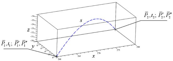
Figure 15. Initial conditions for construction of a Bézier spline curve segment.

Under the given conditions it is possible to construct a Bézier spline curve segment described by the formula [1,10,13]

$$\overline{p}(t)={\displaystyle \sum _{i=0}^n\frac{n!}{i!(n-i)!}{t}^i{(1-t)}^{n-i}}{\overline{A}}_{i+1},n=5,t_1\le t\le t_2,$$

(33)

where the set of functions $B_i^n(t)=\frac{n!}{i!(n-i)!}{t}^i{(1-t)}^{n-i}$ forms the Bernstein basis.

Let us express the first, the second, the third and the fourth derivatives of vector function $\overline{p}(t)$

$$\begin{array}{ll}{\overline{p}}^{\prime }(t)& =-5{(1-t)}^4{\overline{A}}_1+(5{(1-t)}^4-20t{(1-t)}^3){\overline{A}}_2+(20t{(1-t)}^3-30t^2{(1-t)}^2){\overline{A}}_3+\\ & +(30t^2{(1-t)}^2-20t^3(1-t)){\overline{A}}_4+(20t^3(1-t)-5t^4){\overline{A}}_5+5t^4{\overline{A}}_6,\\ {\overline{p}}^{″}(t)& =20{(1-t)}^3{\overline{A}}_1+(-40{(1-t)}^3+60t{(1-t)}^2){\overline{A}}_2+(20{(1-t)}^3-120t{(1-t)}^2+60t^2(1-t)){\overline{A}}_3+\\ & +(60t{(1-t)}^2-120t^2(1-t)+20t^3){\overline{A}}_4+(60t^2(1-t)-40t^3){\overline{A}}_5+20t^3{\overline{A}}_6,\\ {\overline{p}}^{‴}(t)& =-60{(1-t)}^2{\overline{A}}_1+(-120t(1-t)+180{(1-t)}^2){\overline{A}}_2+(-180{(1-t)}^2+360t(1-t)-60t^2){\overline{A}}_3+\\ & +(60{(1-t)}^2+180t^2-360t(1-t)){\overline{A}}_4+(120t(1-t)-180t^2){\overline{A}}_5+60t^2{\overline{A}}_6,\\ {\overline{p}}^{⁗}(t)& =120(1-t){\overline{A}}_1-(480-600t){\overline{A}}_2+(720-1200){\overline{A}}_3-(480-1200t){\overline{A}}_4+\\ & +(120-600t){\overline{A}}_5+120t{\overline{A}}_6.\end{array}$$

Vectors ${\overline{P}}_1^{\prime }$, ${\overline{P}}_2^{\prime }$ are the first vector derivatives constituting tangent vectors at the endpoints of the sought segment s. Vectors ${\overline{P}}_1^{″},{\overline{P}}_2^{″}$ are the second vector derivatives constituting vectors of acceleration of a point tracing out the segment s. Vectors ${\overline{P}}_1^{‴},{\overline{P}}_2^{‴}$ are the third vector derivatives constituting vectors of jerk of a point tracing out the segment s. Vectors ${\overline{P}}_1^{⁗},{\overline{P}}_2^{⁗}$ are the fourth vector derivatives constituting vectors of snap of a point tracing out the segment s.

This allows us to acquire the values of the first three vector coefficients

$$\begin{gathered} \overline{p}(0)={\overline{P}}_1={\overline{A}}_1;{\overline{p}}^{\prime }(0)={\overline{P}}_1^{\prime }=-5{\overline{A}}_1+5{\overline{A}}_2,\mathrm{i}.\mathrm{e}.{\overline{A}}_2=\frac{1}{5}{\overline{P}}_1^{\prime }+{\overline{P}}_1, \\ {\overline{p}}^{″}(0)={\overline{P}}_1^{″}=20{\overline{A}}_1-40{\overline{A}}_2+20{\overline{A}}_3,\mathrm{i}.\mathrm{e}.,{\overline{A}}_3={\overline{P}}_1+\frac{2}{5}{\overline{P}}_1^{\prime }+\frac{1}{20}{\overline{P}}_1^{″}. \end{gathered}$$

(34)

The three remaining vector coefficients are determined through the equations

$$\overline{p}(t_2)={\overline{P}}_2,{\overline{p}}^{\prime }(t_2)={\overline{P}}_2^{\prime },{\overline{p}}^{″}(t_2)={\overline{P}}_2^{″}.$$

(35)

From the Equation (35) follows the system of three linear equations

$$\begin{array}{l}{\displaystyle \sum _{i=0}^5\frac{n!}{i!(n-i)!}{t}^i{(1-t_2)}^{n-i}}{\overline{A}}_{i+1}-{\overline{P}}_2=0,\\ {\displaystyle \sum _{i=0}^5(\frac{120A_{i+1}{t}_2{}^{i}i{(1-t_2)}^{5-i}}{i!(5-i)!t_2}-\frac{120A_{i+1}{t}_2{}^i{(1-t_2)}^{5-i}(5-i)}{i!(5-1)!(1-t_2)})}-{\overline{P}}_2^{\prime }=0,\\ {\displaystyle \sum _{i=0}^5(\begin{array}{c}\frac{120A_{i+1}{t}_2{}^i{i}^2{(1-t_2)}^{5-i}(i-1)}{i!(5-i)!t_2^2}-\frac{240A_{i+1}{t}_2{}^{i}i{(1-t_2)}^{5-i}(5-i)}{i!(5-i)!t_2(1-t_2)}+\\ +\frac{120A_{i+1}{t}_2^i{(1-t_2)}^{5-i}(5-i)((5-i)-1)}{i!(5-i)!{(1-t_2)}^2}\end{array})}-{\overline{P}}_2^{″}=0.\end{array}$$

(36)

The expressions for coefficients ${\overline{A}}_4,{\overline{A}}_5$, and ${\overline{A}}_6$ follow from the system of the Equation (36)

$${\overline{A}}_4=\frac{(t_2^3-1){\overline{P}}_1}{t_2^3}+\frac{{\overline{P}}_2}{t_2^3}+\frac{0.6{\overline{P}}_1^{\prime }}{t_2^3}-\frac{0.4{\overline{P}}_2^{\prime }}{t_2^2}+\frac{0.15(t_2^3-t_2^2){\overline{P}}_1^{″}}{t_2^3}+\frac{0.05{\overline{P}}_2^{″}}{t_2},$$

$$\begin{array}{ll}{\overline{A}}_5& =\frac{(t_2^4-4t_2+3){\overline{P}}_1}{t_2^4}+\frac{(4t_2-3){\overline{P}}_2}{t_2^4}+\frac{(0.8t_2^4-2.4t_2^2+16t_2){\overline{P}}_1^{\prime }}{t_2^4}-\frac{(1.6t_2^2+1.4t_2){\overline{P}}_2^{\prime }}{t_2^4}+\\ & +\frac{0.3(t_2^4-2t_2^3+t_2^2){\overline{P}}_1^{″}}{t_2^4}+\frac{0.2(t_2^3-t_2^2){\overline{P}}_2^{″}}{t_2^4},\end{array}$$

$$\begin{array}{ll}{\overline{A}}_6& =\frac{(t_2^5-10t_2^2+15t_2-6){\overline{P}}_1}{t_2^5}+\frac{(10t_2^2-15t_2-6){\overline{P}}_2}{t_2^5}+\frac{(t_2^5-6t_2^3+8t_2-3){\overline{P}}_1^{\prime }}{t_2^5}-\\ & -\frac{(4t_2^3-7t_2^2+3t_2){\overline{P}}_2^{\prime }}{t_2^5}+\frac{0.5(t_2^5-0.3t_2^4+0.3t_2^3-t_2^2){\overline{P}}_1^{″}}{t_2^5}+\frac{0.5(t_2^4-2t_2^3+t_2^2){\overline{P}}_2^{″}}{t_2^5}.\end{array}$$

The expressions (34) and (36) can be expressed in the matrix form with parameterization $0\le t\le t_2=1$

$$\left[\overline{A}\right]=\left[\begin{array}{c}{\overline{A}}_1\\ {\overline{A}}_2\\ {\overline{A}}_3\\ {\overline{A}}_4\\ {\overline{A}}_5\\ {\overline{A}}_6\end{array}\right]=\left[\begin{array}{cccccc}1& 0& 0& 0& 0& 0\\ 1& 0& \frac{1}{5}& 0& 0& 0\\ 1& 0& \frac{2}{5}& 0& \frac{1}{20}& 0\\ 0& 1& 0& -\frac{2}{5}& 0& \frac{1}{20}\\ 0& 1& 0& -\frac{1}{5}& 0& 0\\ 0& 1& 0& 0& 0& 0\end{array}\right]\cdot \left[\begin{array}{c}{\overline{P}}_1\\ {\overline{P}}_2\\ {\overline{P}}_1^{\prime }\\ {\overline{P}}_2^{\prime }\\ {\overline{P}}_1^{″}\\ {\overline{P}}_2^{″}\end{array}\right].$$

(37)

3.7. Construction of a Fifth-Degree Bézier Spline Curve of Two Segments

Let us consider the connection of two segments of a fifth-degree Bézier spline curve (see Figure 16) given the same boundary conditions as for the case of one segment s previously considered in Section 3.6.

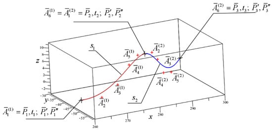
Figure 16. Knot and control points of two connected segments of a fifth-degree Bézier spline curve.

Let us express the equation of the segments in the following form: ${\overline{p}}_k(t)={\displaystyle \sum _{i=0}^{n=5}\frac{n!}{i!(n-i)!}{t}^i{(1-t)}^{5-i}}{\overline{A}}_{i+1}^{(k)}$; $k=1,2$, $0\le t\le 1$. A Bézier spline segment has control points ${\overline{A}}_2^{(k)}$, ${\overline{A}}_3^{(k)}$, ${\overline{A}}_4^{(k)}$, ${\overline{A}}_5^{(k)}$ and passes through knot points ${\overline{A}}_1^{(k)}={\overline{P}}_k$, ${\overline{A}}_6^{(k)}={\overline{P}}_{k+1}$.

For k = 1 at the initial point ${\overline{P}}_1(t_1=0)$ of segment $s_1$ we acquire

$${\overline{p}}_1(0)={\overline{P}}_1={\overline{A}}_1^{(1)},{\overline{p}}_1^{\prime }(0)={{\overline{P}}^{\prime }}_1=5(-{\overline{A}}_1^{(1)}+{\overline{A}}_2^{(1)}),{\overline{p}}_1^{″}(0)={\overline{P}}_1^{″}=20({\overline{A}}_1^{(1)}-2{\overline{A}}_2^{(1)}+{\overline{A}}_3^{(1)}).$$

(38)

For k = 1 at the final point ${\overline{P}}_2(t_2=1)$ of segment $s_1$ we acquire

$${\overline{p}}_1(1)={\overline{P}}_2={\overline{A}}_6^{(1)},{\overline{p}}_1^{\prime }(1)={\overline{P}}_2^{\prime }=5(-{\overline{A}}_5^{(1)}+{\overline{P}}_2),{\overline{p}}_1^{″}(1)={\overline{P}}_2^{″}=20({\overline{A}}_4^{(1)}-2{\overline{A}}_5^{(1)}+{\overline{P}}_2).$$

For k = 2 at the initial point ${\overline{P}}_2(t_2=0)$ of segment $s_2$ we acquire

$${\overline{p}}_2(0)={\overline{P}}_2={\overline{A}}_1^{(2)},{\overline{p}}_2^{\prime }(0)={\overline{P}}_2^{\prime }=5(-{\overline{A}}_1^{(2)}+{\overline{A}}_2^{(2)}),{\overline{p}}_2^{″}(0)={\overline{P}}_2^{″}=20({\overline{A}}_1^{(2)}-2{\overline{A}}_2^{(2)}+{\overline{A}}_3^{(2)})$$

(39)

At the final point ${\overline{P}}_3(t_3=1)$ of segment $s_2$ we acquire

$${\overline{p}}_2(1)={\overline{P}}_3={\overline{A}}_6^{(2)},{\overline{p}}_2^{\prime }(1)={\overline{P}}_3^{\prime }=5(-{\overline{A}}_5^{(2)}+{\overline{P}}_3),{\overline{p}}_2^{″}(1)={\overline{P}}_3^{″}=20({\overline{A}}_4^{(2)}-2{\overline{A}}_5^{(2)}+{\overline{P}}_3).$$

It is required to determine eight vector coefficients corresponding to vectors of the four control points of each segment. At the initial point of segment $s_1$ and the final point of segment $s_2$ the following boundary conditions are given: ${\overline{P}}_1^{\prime }$, ${\overline{P}}_1^{″}$ and ${\overline{P}}_3^{\prime }$, ${\overline{P}}_3^{″}$. Therefore, through (38), we acquire the expressions for the first three vector coefficients of the equation for the first segment $s_1$: ${\overline{A}}_1^{(1)}={\overline{P}}_1$, ${\overline{A}}_2^{(1)}=\frac{1}{5}{\overline{P}}_1^{\prime }+{\overline{P}}_1$ and ${\overline{A}}_3^{(1)}=\frac{1}{20}{\overline{P}}_1^{″}+{\overline{P}}_1+\frac{2}{5}{\overline{P}}_1^{\prime }$. The remaining vector coefficients ${\overline{A}}_4^{(1)},{\overline{A}}_5^{(1)}$, and ${\overline{A}}_6^{(1)}$ are determined through the system of three linear equations

$$\{\begin{array}{l}{\overline{A}}_6^{(1)}-{\overline{P}}_2=0,\\ -5({\overline{A}}_5^{(1)}-{\overline{A}}_6^{(1)})-{\overline{P}}_2^{\prime }=0,\\ 20({\overline{A}}_4^{(1)}-2{\overline{A}}_5^{(1)}+{\overline{A}}_6^{(1)})-{\overline{P}}_2^{″}=0.\end{array}$$

(40)

Through (39) we acquire the expressions for the first three vector coefficients of the equation for the second segment $s_2$: ${\overline{A}}_1^{(2)}={\overline{P}}_2$, ${\overline{A}}_2^{(2)}=\frac{1}{5}{\overline{P}}_2^{\prime }+{\overline{P}}_2$, ${\overline{A}}_3^{(2)}=\frac{1}{20}{\overline{P}}_2^{″}+{\overline{P}}_2+\frac{2}{5}{\overline{P}}_2^{\prime }$. The remaining vector coefficients ${\overline{A}}_4^{(2)},{\overline{A}}_5^{(2)}$, and ${\overline{A}}_6^{(2)}$ are determined through the system of three linear equations

$$\{\begin{array}{l}{\overline{A}}_6^{(2)}-{\overline{P}}_3=0,\\ -5({\overline{A}}_5^{(2)}-{\overline{A}}_6^{(2)})-{\overline{P}}_3^{\prime }=0,\\ 20({\overline{A}}_4^{(2)}-2{\overline{A}}_5^{(2)}+{\overline{A}}_6^{(2)})-{\overline{P}}_3^{″}=0.\end{array}$$

(41)

In the connection of segments $s_1$ and $s_2$ at the point $P_2$ with smoothness $C^4$, vectors ${\overline{P}}_2^{\prime }$ and ${\overline{P}}_2^{″}$ are unknown. These vectors are determined through the condition of equality of the third and the fourth derivatives of vector functions of the segments at the connection point: ${\overline{p}}_1^{‴}(t=1)={\overline{p}}_2^{‴}(t=0)$, or in expanded form

$$-60({\overline{A}}_3^{(1)}+3{\overline{A}}_4^{(1)}-3{\overline{A}}_5^{(1)})=-60(3{\overline{A}}_2^{(2)}-3{\overline{A}}_3^{(2)}+3{\overline{A}}_4^{(2)}),$$

(42)

and ${\overline{p}}_1^{⁗}(t=1)={\overline{p}}_2^{⁗}(t=0)$, or in expanded form

$$120({\overline{A}}_2^{(1)}-4{\overline{A}}_3^{(1)}+6{\overline{A}}_4^{(1)}-4{\overline{A}}_5^{(1)})=120(-4{\overline{A}}_2^{(2)}+6{\overline{A}}_3^{(2)}-4{\overline{A}}_4^{(2)}+4{\overline{A}}_5^{(2)}).$$

(43)

The sought vectors ${\overline{P}}_2^{\prime }$ and ${\overline{P}}_2^{″}$ are determined through the system of two linear Equations (43) and (44) taking into account the system of Equations (39)–(42)

$${\overline{P}}_2^{\prime }=\frac{1}{16}(-7{\overline{P}}_1^{\prime }-15{\overline{P}}_1-7{\overline{P}}_3^{\prime }+15{\overline{P}}_3-{\overline{P}}_1^{″}+{\overline{P}}_3^{″}).$$

(44)

$${\overline{P}}_2^{″}=\frac{1}{3}(-20{\overline{P}}_2+4{\overline{P}}_1^{\prime }+10{\overline{P}}_1-4{\overline{P}}_3^{\prime }+10{\overline{P}}_3+\frac{1}{2}{\overline{P}}_1^{″}+\frac{1}{2}{\overline{P}}_3^{″}).$$

(45)

The Equations (44) and (45) in calculation of the unknown vector derivatives ${\overline{P}}_2^{\prime }$ and ${\overline{P}}_2^{″}$ at the point of connection of fifth-degree Bézier spline curve segments $s_1$ and $s_2$ match the corresponding Equations (9) and (10) of the unknown vector derivatives ${\overline{P}}_2^{\prime }$ and ${\overline{P}}_2^{″}$ at the point of connection of fifth-degree Hermite spline curve segments $s_1$ and $s_2$. In this case, in the Formulas (9) and (10), the coefficients $k_r(t),n_r(t),r=1,\dots ,7;\alpha ,\beta$ take values according to (11) for $0\le t\le 1$.

This allows us to speak of universality of the proposed algorithm of determination of the unknown vector derivatives in the tasks of formation of various polynomial curves. Thus, the vector derivatives ${\overline{P}}_2^{\prime }$ and ${\overline{P}}_2^{″}$ at the points of connection of fifth-degree Bézier spline curve segments are determined through the Equations (9) and (10), same as for the case of a Hermite spline curve. However, the acquired equations for the unknown vector coefficients of Bézier spline curves and Hermite spline curves are different. The unknown vector coefficients ${\overline{A}}_i^{(k)},k=1,\dots ,n;i=1,\dots ,6$ corresponding to the control points of the composite Bézier spline curve are calculated through (46). The generalized matrix form $\left[\overline{A}\right]=\left[T\right]\cdot \left[\overline{G}\right]$ for calculating vector coefficients ${\overline{A}}_i^k$ for a non-closed fifth-degree Bézier spline has the form

$$\left[\overline{A}\right]=\left[\begin{array}{l}{\overline{A}}_1^{(1)}\\ {\overline{A}}_2^{(1)}\\ {\overline{A}}_3^{(1)}\\ {\overline{A}}_4^{(1)}\\ {\overline{A}}_5^{(1)}\\ {\overline{A}}_6^{(1)}\\ \dots \\ {\overline{A}}_1^{(j-1)}\\ {\overline{A}}_2^{(j-1)}\\ {\overline{A}}_3^{(j-1)}\\ {\overline{A}}_4^{(j-1)}\\ {\overline{A}}_5^{(j-1)}\\ {\overline{A}}_6^{(j-1)}\end{array}\right]=\left[\begin{array}{ccccccccccccccc}1& 0& \dots & 0& 0& 0& 0& \dots & 0& 0& 0& 0& \dots & 0& 0\\ 1& 0& \dots & 0& 0& \frac{1}{5}& 0& \dots & 0& 0& 0& 0& \dots & 0& 0\\ 1& 0& \dots & 0& 0& \frac{2}{5}& 0& \dots & 0& 0& \frac{1}{20}& 0& \dots & 0& 0\\ 0& 1& \dots & 0& 0& 0& -\frac{2}{5}& \dots & 0& 0& 0& \frac{1}{20}& \dots & 0& 0\\ 0& 1& \dots & 0& 0& 0& -\frac{1}{5}& \dots & 0& 0& 0& 0& \dots & 0& 0\\ 0& 1& \dots & 0& 0& 0& 0& \dots & 0& 0& 0& 0& \dots & 0& 0\\ \dots & \dots & \dots & \dots & \dots & \dots & \dots & \dots & \dots & \dots & \dots & \dots & \dots & \dots & \dots \\ 0& 0& \dots & 1& 0& 0& 0& \dots & 0& 0& 0& 0& \dots & 0& 0\\ 0& 0& \dots & 1& 0& 0& 0& \dots & \frac{1}{5}& 0& 0& 0& \dots & 0& 0\\ 0& 0& \dots & 1& 0& 0& 0& \dots & \frac{2}{5}& 0& 0& 0& \dots & \frac{1}{20}& 0\\ 0& 0& \dots & 0& 1& 0& 0& \dots & 0& -\frac{2}{5}& 0& 0& \dots & 0& \frac{1}{20}\\ 0& 0& \dots & 0& 1& 0& 0& \dots & 0& -\frac{1}{5}& 0& 0& \dots & 0& 0\\ 0& 0& \dots & 0& 1& 0& 0& \dots & 0& 0& 0& 0& \dots & 0& 0\end{array}\right]\cdot \left[\begin{array}{c}{\overline{P}}_1\\ {\overline{P}}_2\\ \dots \\ {\overline{P}}_{j-1}\\ {\overline{P}}_j\\ {\overline{P}}_1^{\prime }\\ {\overline{P}}_2^{\prime }\\ \dots \\ {\overline{P}}_{j-1}^{\prime }\\ {\overline{P}}_j^{\prime }\\ {\overline{P}}_1^{″}\\ {\overline{P}}_2^{″}\\ \dots \\ {\overline{P}}_{j-1}^{″}\\ {\overline{P}}_j^{″}\end{array}\right].$$

(46)

Example 6.

The following conditions for the three segments are given:${\overline{P}}_1(0,50,0)$,${\overline{P}}_2(150,100,50)$,${\overline{P}}_3(250,200,60)$,${\overline{P}}_4(300,300,0)$,${\overline{P}}_1^{\prime }(-50,100,1)$,${\overline{P}}_4^{\prime }(301,-210,-1)$,${\overline{P}}_1^{″}(50,-100,2)$,${\overline{P}}_4^{″}(280,-280,1)$. It is required to construct a Bézier spline curve of these segments. The unknown vector derivatives${\overline{P}}_2^{\prime },{\overline{P}}_2^{″},{\overline{P}}_3^{\prime }$and${\overline{P}}_3^{″}$at the points of connection of the segments are calculated as in the case of a smooth connection of three segments for a Hermite spline curve of the fifth degree consisting of three segments (see Example 1). The unknown vector coefficients${\overline{A}}_i^{(k)},k=1,\dots ,3;i=1,\dots ,6$are calculated through (46).

Figure 17 depicts visual rendering of the result of the calculation. It demonstrates the sought three segments of a Bézier spline curve and their subsequent connection with smoothness $C^4$.

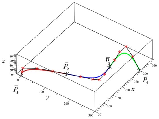
Figure 17. Fifth-degree Bézier spline curve of three segments.

Table 6 lists the values of curvature and torsion at the boundary points ${\overline{P}}_j$ of the connected segments, where j = 1, …, 4.

Table 6. Curvature and torsion values at boundary points of the segments.

Segment	Segment Boundary Knot Point ${\overline{\mathit{P}}}_{\mathit{j}}$	Curvature Value	Torsion Value
$s_1:{\overline{p}}_1(t)$	${\overline{P}}_1$, t = 0	0.0002399712029	8.722088677
	${\overline{P}}_2$, t = 1	0.0003181576505	0.02375800221
$s_2:{\overline{p}}_2(t)$	${\overline{P}}_2$, t = 0	0.0003181576505	0.02375800221
	${\overline{P}}_3$, t = 1	0.001200350474	−0.01488694419
$s_3:{\overline{p}}_3(t)$	${\overline{P}}_3$, t = 0	0.001200350474	−0.01488694419
	${\overline{P}}_4$, t = 1	0.0005156220501	0.04777943587

Example 7.

It is required to construct a closed fifth-degree Bézier spline curve of five segments subsequently connected in knot points${\overline{P}}_1(0,0,0)$,${\overline{P}}_2(0,100,10)$,${\overline{P}}_3(100,50,20)$,${\overline{P}}_4(100,300,100)$,${\overline{P}}_5(300,0,0)$.

The unknown vector derivatives ${\overline{P}}_j^{\prime }$ and ${\overline{P}}_j^{″}$, j = 1,…,5 are determined through the matrix form of the generalized system of Equation (17). This is due to the fact that the calculation of the unknown vector derivatives ${\overline{P}}_j^{\prime }$ and ${\overline{P}}_j^{″}$ at the connection points of Hermite and Bézier spline segments are formally identical.

The system of equations for the unknown vector derivatives for the current example is of the following matrix form:

$$\begin{array}{l}\\ \begin{array}{cccccccccccc}{\overline{P}}_1^{\prime }& {\overline{P}}_2^{\prime }& {\overline{P}}_3^{\prime }& {\overline{P}}_4^{\prime }& {\overline{P}}_5^{\prime }& {\overline{P}}_1^{″}& {\overline{P}}_2^{″}& {\overline{P}}_3^{″}& {\overline{P}}_4^{″}& {\overline{P}}_5^{″}& & \\ 7& 16& 7& 0& 0& 1& 0& -1& 0& 0& & -15({\overline{P}}_1-{\overline{P}}_3)\\ 4& 0& -4& 0& 0& \frac{1}{2}& -3& \frac{1}{2}& 0& 0& & -10({\overline{P}}_1-2{\overline{P}}_2+{\overline{P}}_3)\\ 0& 7& 16& 7& 0& 0& 1& 0& -1& 0& & -15({\overline{P}}_2-{\overline{P}}_4)\\ 0& 4& 0& -4& 0& 0& \frac{1}{2}& -3& \frac{1}{2}& 0& & -10({\overline{P}}_2-2{\overline{P}}_3+{\overline{P}}_4)\\ 0& 0& 7& 16& 7& 0& 0& 1& 0& -1& & -15({\overline{P}}_3-{\overline{P}}_5)\\ 0& 0& 4& 0& -4& 0& 0& \frac{1}{2}& -3& \frac{1}{2}& & -10({\overline{P}}_3-2{\overline{P}}_4+{\overline{P}}_5)\\ 7& 0& 0& 7& 16& -1& 0& 0& 1& 0& & -15({\overline{P}}_4-{\overline{P}}_1)\\ -4& 0& 0& 4& 0& \frac{1}{2}& 0& 0& \frac{1}{2}& -3& & -10({\overline{P}}_4-2{\overline{P}}_5+{\overline{P}}_1)\\ 16& 7& 0& 0& 7& 0& -1& 0& 0& 1& & -15({\overline{P}}_5-{\overline{P}}_2)\\ 0& -4& 0& 0& 4& -3& \frac{1}{2}& 0& 0& \frac{1}{2}& & -10({\overline{P}}_5-2{\overline{P}}_1+{\overline{P}}_2)\end{array}\end{array}$$

The unknown vector coefficients ${\overline{A}}_i^{(k)},k=1,\dots ,5;i=1,\dots ,6$ are calculated through the system of Equation (46) expanded by adding a closing segment equation containing the vector coefficients ${\overline{A}}_i^{(k)},i=1,\dots ,6$.

Figure 18 and Table 7 present the results of the construction of a closed fifth-degree Bézier spline curve of five segments.

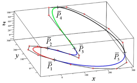
Figure 18. Closed fifth-degree Bézier spline curve of five segments.

Table 7. Curvature and torsion values at boundary points of the segments.

Segment	Segment Boundary Knot Point ${\overline{\mathit{P}}}_{\mathit{j}}$	Curvature Value	Torsion Value
$s_1:{\overline{p}}_1(t)$	${\overline{P}}_1$, t = 0	0.003100353669	0.0005995357794
	${\overline{P}}_2$, t = 1	0.006264502175	–0.001862804412
$s_2:{\overline{p}}_2(t)$	${\overline{P}}_2$, t = 0	0.006264502175	–0.001862804412
	${\overline{P}}_3$, t = 1	0.003451401672	–0.01338727745
…	…	…	…
$s_4:{\overline{p}}_4(t)$	${\overline{P}}_4$, t = 0	0.02757323507	–0.0001744660457
	${\overline{P}}_5$, t = 1	0.008921353117	0.0001689425348
$s_5:{\overline{p}}_5(t)$	${\overline{P}}_5$, t = 0	0.008921353117	0.0001689425348
	${\overline{P}}_1$, t = 1	0.003100353669	0.0005995357794

The mathematical models of shaping of Bézier spline curves obtained in Section 3.6 and Section 3.7 also have scientific novelty. These models were not previously considered in the scientific literature on computational geometry known to the authors.

The considered examples were tested using the software package of the Waterloo Maple computer mathematics system—Maple 2020 Free Trial. Access to the computer code for the examples No.1–No.7 considered in the work is possible by the link: https://www.mapleprimes.com/posts/213421-Spline-Curves-Formation-Given-Extreme-Derivatives?sp=213421.

4. Discussion

The mathematical models of formation of various polynomial spline curves considered in Section 3 determine the computational algorithms of formation. These algorithms are validated on numerous examples provided in Section 3. The uniformity and systematic nature of the algorithms allows us to present them in the form of a general algorithm of spline curve formation (see Figure 19).

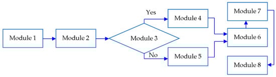
Figure 19. General algorithm of spline curve formation.

This general algorithm allows us to perform calculation of vector derivatives at points of connection of segments forming a spline curve as well as vector coefficients of polynomials. The algorithm consists of modules providing the following functions:

Module 1: Initial conditions input. The initial conditions for spline curve formation include: the number of points of discrete array j; the vectors of discrete array of points ${\overline{P}}_1,\dots ,{\overline{P}}_j$; the number of pairs of extreme derivatives m; the vectors of extreme derivatives ${\overline{P}}_1^{\prime },{\overline{P}}_1^{″},{\overline{P}}_1^{‴}\dots$ at point ${\overline{P}}_1$; the vectors of extreme derivatives ${\overline{P}}_j^{\prime },{\overline{P}}_j^{″},{\overline{P}}_j^{‴}\dots$ at point ${\overline{P}}_j$.

Module 2: Determination of order $n=2m+1$ of the polynomial.

Module 3: Conditional step: check whether the curve is closed. The curve is considered closed if the vectors of extreme derivatives at points ${\overline{P}}_1$ and ${\overline{P}}_j$ are not given as the initial conditions.

Module 4: Formation of a matrix of size $((N-j)\times (N-j))$ for the unknown vector derivatives at connection points of a closed spline curve, where $N$ represents the total number of conditions.

Module 5: Formation of a matrix of size $((N-(2m+j))\times (N-(2m+j)))$ for the unknown vector derivatives at connection points of a non-closed spline curve, where $N$ represents the total number of conditions.

Module 6: Calculation of vector derivatives at segment connection points.

Module 7: Calculation of polynomial vector coefficients for each spline curve segment.

Module 8: Acquiring the vector equations of spline curve segments.

Aside from uniformity, the proposed algorithms are to a certain extent universal and can be applied in solutions to the problems of formation of polynomial spline curves of various types generated through Hermite splines, Bézier splines, B-splines. It has to be mentioned that the Gauss–Jordan method has time complexity $O(i^3+(\log p)i)$, where p is the size of the initial data for solution of a system of i equations in i unknown. These systems are present in every computational algorithm proposed in Section 3.

Analysis of Algorithms 1–3 (Section 3.2, Section 3.5, and Section 3.7, respectively), analysis of matrices for the formation of vector coefficients in the equations of segments of formed spline curves (Section 3.1, Section 3.2, Section 3.3, Section 3.4, Section 3.5, Section 3.6 and Section 3.7) and analysis of the set of considered numerical examples (examples 1–7, Table 1, Table 2, Table 3, Table 4, Table 5, Table 6 and Table 7) allow us to conclude about the scalability of our proposed method of forming spline curves. The scalability of the method is reduced to the obvious scalability of the matrices of vector coefficients of the segment equations, the connection of which, according to a given degree of smoothness, forms a certain spline curve.

The accuracy of the obtained computational results depends on the specified computation accuracy of scalar invariants at the segments junction point and does not depend on the scalability of the proposed computation method. The examples discussed in the work (electronic link on Page 27) support this thesis. For a given accuracy of calculations (100 decimal places) of an open spline of the Hermite curve of the fifth degree, the resulting absolute calculation error is from 10⁻⁹⁹ to 10⁻⁹⁴. As an example, the formation of a spline curve consisting of 100 knots is considered. In this case, the obtained absolute error in calculating the curvature at the segments joining knots is as follows: knot ${\overline{P}}_2:5.31\cdot {10}^{-99}$,..., knot ${\overline{P}}_{50}:2.4\cdot {10}^{-99}$,..., knot ${\overline{P}}_{99}:3.0\cdot {10}^{-100}$. The obtained absolute error in the calculation of the torsion at the knots of joining the segments is as follows: knot ${\overline{P}}_2:9.59\cdot {10}^{-94}$,…, knot ${\overline{P}}_{50}:1.05\cdot {10}^{-97}$,…, knot ${\overline{P}}_{99}:1.73\cdot {10}^{-97}$. The accuracy of calculating scalar invariants can be quite high, depending on practical feasibility, as well as on the capabilities of the computer hardware.

Algorithm 3 For obtaining a fifth-degree Bézier spline curve of segments $s_1$ and $s_2$ has the following text form:

Vector derivatives ${\overline{P}}_2^{\prime }$ and ${\overline{P}}_2^{″}$ at the joining point ${\overline{P}}_2$ of segments $s_1$ and $s_2$ are determined based on the Formulas (44) and (45). Determine the vector coefficients ${\overline{A}}_i^{(1)}$ in the segment equation $s_1$ based on the matrix (37). In this case, the boundary conditions of the segment $s_1$ are the given vector derivatives ${\overline{P}}_1^{\prime }$ and ${\overline{P}}_1^{″}$ at the knot ${\overline{P}}_1$ and the vector derivatives ${\overline{P}}_2^{\prime }$ and ${\overline{P}}_2^{″}$ at the knot ${\overline{P}}_2$ determined according to item 1. Determine the vector coefficients ${\overline{A}}_i^{(2)}$ in the segment equation $s_2$ based on matrix (37). In this case, the boundary conditions of the segment $s_2$ are the vector derivatives ${\overline{P}}_2^{\prime }$ and ${\overline{P}}_2^{″}$ at the knot ${\overline{P}}_2$ determined according to item 1 and the given vector derivatives ${\overline{P}}_3^{\prime }$ and ${\overline{P}}_3^{″}$ at the knot ${\overline{P}}_3$.

5. Conclusions

Vector derivatives form scalar invariants at each regular point of curve $\overline{p}=\overline{p}(t)$, ${\overline{p}}^{(1)}(t)=\frac{d\overline{p}}{dt}\ne 0$. Scalar invariants formed by vector derivatives ${\overline{p}}^{(1)}$,${\overline{p}}^{(2)}$,${\overline{p}}^{(3)}$,...,${\overline{p}}^{(m)}$ have to meet certain requirements. They have to be coordinate system independent, i.e., invariant with respect to coordinate system transformation; they have to be independent of transformations of parameter $t=f(t^{\ast })$, where $f$ is an analytic function of form

$$\overline{p}(t)=\overline{p}(f(t^{\ast }))={\overline{p}}^{\ast }(t^{\ast }),d{\overline{p}}^{\ast }(t^{\ast })=\frac{d\overline{p}}{dt}{f}^{(1)},f^{(1)}=\frac{df}{d{t}^{\ast }}\ne 0.$$

The formation of scalar invariants of a curve can be considered on the following examples: scalar invariants of the first order (by the highest order of the applied vector derivatives) ${({\overline{p}}^{(1)}(t))}^2$, scalar invariants of the second order (curvature) $k(t)=G({\overline{p}}^{(1)}(t),{\overline{p}}^{(2)}(t))=G^{\ast }(t)$, scalar invariants of the third order (torsion) $\chi (t)=F({\overline{p}}^{(1)}(t),{\overline{p}}^{(2)}(t),{\overline{p}}^{(3)}(t))=F^{\ast }(t)$. It is obvious that the scalar invariants of the segments have to be equal at the points of smooth connection of spline curve segments. Let us consider smooth connection of adjacent segments $s_k$ and $s_{k+1}$ of the constructed spline

$$s_k:{\overline{p}}_k(t_k)={\displaystyle \sum _{i=1}^n{\overline{A}}_{i(k)}}{t}_k^{i-1},t_k\in [0,T_k],$$

$$s_{k+1}:{\overline{p}}_{k+1}(t_{k+1})={\displaystyle \sum _{i=1}^n{\overline{A}}_{i(k+1)}}{t}_{k+1}^{i-1},t_{k+1}\in [0,T_{k+1}].$$

Let us express in general form the scalar functions of vector arguments (derivatives) of the segments $s_k$ and $s_{k+1}$

$$H({\overline{p}}_k^{(1)}(t_k),{\overline{p}}_k^{(2)}(t_k),\dots ,{\overline{p}}_k^{(m)}(t_k))=H^{\ast }(t_k).$$

(47)

$$V({\overline{p}}_{k+1}^{(1)}(t_{k+1}),{\overline{p}}_{k+1}^{(2)}(t_{k+1}),\dots ,{\overline{p}}_{k+1}^{(m)}(t_{k+1}))=V^{\ast }(t_{k+1}).$$

(48)

The scalar functions (47) and (48) are of the equivalent mathematical form, i.e., they accept the equivalent set of vector arguments (derivatives) and perform the equivalent set of mathematical operations over said arguments.

In order to achieve connections of segments $s_k$ and $s_{k+1}$ with smoothness $C^m$, it is necessary to satisfy the following conditions:

$$\begin{array}{l}{\overline{p}}_k^{(1)}(t_k=T_k)={\overline{p}}_{k+1}^{(1)}(t_{k+1}=0),\\ {\overline{p}}_k^{(2)}(t_k=T_k)={\overline{p}}_{k+1}^{(2)}(t_{k+1}=0),\\ {\overline{p}}_k^{(m)}(t_k=T_k)={\overline{p}}_{k+1}^{(m)}(t_{k+1}=0).\end{array}$$

(49)

In that case, the Equation (49) and the equivalence of the mathematical form of the scalar functions (47) and (48) result in the equality of values $H^{\ast }(t_k=T_k)=V^{\ast }(t_{k+1}=0)$ that effectively means the equality of scalar invariants at the point of connection with smoothness $C^m$.

What does this mean? It means that formation of splines through smooth connection of segments described by polynomials of higher degree determines objective existence of scalar invariants of orders higher than three (as for the case of torsion) at the connection point. These invariants generate multidimensional number space of scalar invariants of segmentally formed spline curves. It has not been studied previously. To study this space for completeness and practicality is the objective of further development of the spline formation problem considered in the present paper. We believe that further study of algorithms for the formation of scalar invariants of high orders and mathematical manipulation of these invariants in the indicated space will contribute to the appearance of spline curves of a new level of quality. As for the precision of calculation of second- and third-order scalar invariants (curvature and torsion), the calculation results provided in Table 1, Table 2, Table 3, Table 4, Table 5, Table 6 and Table 7 show that it can be sufficiently high and is determined on the grounds of practicality.

References

- Salomon, D. Curves and Surfaces for Computer Graphics; Springer Science+Business Media, Inc.: New York, NY, USA, 2006; pp. 11–164. [Google Scholar]
- Zhong, W.B.; Luo, X.C.; Chang, W.L.; Cai, Y.K.; Ding, F.; Liu, H.T.; Sun, Y.Z. Toolpath interpolation and smoothing for computer numerical control machining of freeform surfaces: A review. Int. J. Autom. Comput. 2020, 17, 1–16. [Google Scholar] [CrossRef]
- Sorokin, V.; Kombarov, V. Sravnenie kinematicheskix parametrov dvizheniya pri modelirovanii traektorij vy‘sokoskorostnoj CHPu obrabotki splajnami tret‘ej i pyatoj stepenej. [Comparison of the kinematic parameters of motion when modeling the trajectories of high-speed CNC machining with splines of the third and fifth degrees]. Aerosp. Eng. Technol. 2012, 8, 11–17. [Google Scholar]
- Kombarov, V.; Sorokin, V.; Fojtů, O.; Aksonov, Y.; Kryzhyvets, Y. S-curve algorithm of acceleration/deceleration with smoothlylimited jerk in high-speed equipment control tasks. MM Sci. J. 2019, 2019, 3264–3270. [Google Scholar] [CrossRef]
- Shen, X.; Xie, F.; Liu, X.J.; Xie, Z. A smooth and undistorted toolpath interpolation method for 5-DoF parallel kinematic machines. Robot. Comput. Integr. Manuf. 2019, 57, 347–356. [Google Scholar] [CrossRef]
- Mellinger, D.; Kumar, V. Minimum snap trajectory generation and control for quadrotors. In Proceedings of the 2011 IEEE International Conference on Robotics and Automation, Shanghai, China, 9–13 May 2011; pp. 2520–2525. [Google Scholar]
- Smulsky, J.J.; Smulsky, Y.J. Asteroids Apophis and 1950 DA: 1000 years orbit evolution and possible use. Horiz. Earth Sci. Res. 2012, 6, 63–97. [Google Scholar]
- Smulsky, J.J.; Smulsky, Y.J. Asteroid Apophis: Orbital Evolution and Possible Uses. Colon. Space 2014, 10, 1–17. [Google Scholar]
- Farouki, R.T. Pythagorean-Hodograph Curves: Algebra and Geometry Inserparable; Springer: Berlin/Heidelberg, Germany, 2008; pp. 323–552. [Google Scholar]
- Agoston, M.K. Computer Graphics and Geometric Modeling; Springer: London, UK, 2005; pp. 373–470. [Google Scholar]
- Shikin, E.V.; Plis, A.I. Krivy‘e i Poverxnosti na E‘Krane Komp‘Yutera [Curves and Surfaces on a Computer Screen]; Dialog-Mifi: Moscow, Russia, 1996; pp. 90–150. [Google Scholar]
- Farin, G. Curves and Surfaces for Computer Aided Geometric Design. Implementation and Algorithms, A Practical Guide, 4th ed.; Academic Press: San Diego, CA, USA, 1997; pp. 44–140. [Google Scholar]
- Farin, G.; Hoschek, J.; Kim, M.S. Handbook of Computer Aided Geometric Design; Elsevier Science B.V.: Amsterdam, The Netherlands, 2002; pp. 75–87. [Google Scholar]
- Knott, G.D. Interpolating Cubic Splines; Birkhauser: Boston, MA, USA, 1999; pp. 63–178. [Google Scholar]
- Hirz, M.; Dietrich, W.; Gfrerrer, A.; Lang, J. Integrated Computer-Aided Design in Automotive Development; Springer: Berlin/Heidelberg, Germany, 2013; pp. 86–136. [Google Scholar]
- Bartels, R.H.; Beatty, J.C.; Barsky, B.A. An Introduction to Splines for Use in Computer Graphics and Geometric Modeling; Morgan Kaufmann Publishers, Inc.: Los Altos, CA, USA, 1987; pp. 9–17. [Google Scholar]
- Kornishin, M.S.; Pajmushin, V.N.; Snigirev, V.F. Vy‘chislitel‘naya Geometriya v Zadachax Mexaniki Obolochek [Computational Geometry in Problems of Shell Mechanics]; Nauka: Moscow, Russia, 1989; pp. 28–53. [Google Scholar]
- Gallier, J. Curves and Surfaces in Geometric Modeling: Theory and Algorithms; University of Pennsylvania: Philadelphia, PA, USA, 2018; pp. 61–114. [Google Scholar]
- Rogers, D.F.; Adams, J.A. Mathematical Elements for Computer Graphics, 2nd ed.; McGraw-Hill: New York, NY, USA, 1990; pp. 247–289. [Google Scholar]
- Piegl, L.A.; Tiller, W. Curve interpolation with arbitrary and derivatives. Eng. Comput. 2000, 16, 73–79. [Google Scholar] [CrossRef]
- Marsh, D. Applied Geometry for Computer Graphics and CAD, 2nd ed.; Springer: London, UK, 2005; pp. 135–185. [Google Scholar]
Publisher’s Note: MDPI stays neutral with regard to jurisdictional claims in published maps and institutional affiliations. |
© 2020 by the authors. Licensee MDPI, Basel, Switzerland. This article is an open access article distributed under the terms and conditions of the Creative Commons Attribution (CC BY) license (http://creativecommons.org/licenses/by/4.0/).