A pde-Based Analysis of the Spectrogram Image for Instantaneous Frequency Estimation

Abstract

Instantaneous frequency (IF) is a fundamental feature in multicomponent signals analysis and its estimation is required in many practical applications. This goal can be successfully reached for well separated components, while it still is an open problem in case of interfering modes. Most of the methods addressing this issue are parametric, that is, they apply to a specific IF class. Alternative approaches consist of non-parametric time filtering-based procedures, which do not show robustness to destructive interference—the most critical scenario in crossing modes. In this paper, a method for IF curves estimation is proposed. The case of amplitude and frequency modulated two-component signals is addressed by introducing a spectrogram time-frequency evolution law, whose coefficients depend on signal IFs time derivatives, that is, the chirp rates. The problem is then turned into the resolution of a two-dimensional linear system which provides signal chirp rates; IF curves are then obtained by a simple integration. The method is non-parametric and it results quite robust to destructive interference. An estimate of the estimation error, as well as a numerical study concerning method sensitivity and robustness to noise are also provided in the paper.

1. Introduction

Instantaneous frequency (IF) estimation is of great interest in many applications dealing with non-stationary signals, such as radar and Micro Doppler systems [1,2,3], seismic signals [4], some kinds of gravitational waves [5,6], audio [7] and human speech signals [8], animal sounds [9] and biomedical signals [10]. Practical applications deal with multicomponent signals (MCS), that is, the superposition of individual waveforms, characterized by specific time-dependent frequency content, that is, IF, as well as time-dependent amplitude, namely the instantaneous amplitude (IA) [11]. The correct analysis of MCS requires signal modes separation, that also allows for IFs estimation. Conversely, in many decomposition schemes, IFs estimation is a required step for the recovery of the individual modes by the observed mixture.

It is worth pointing out that IFs detection becomes a very challenging task if signal modes interfere with each other. That is why most of IF estimators in the literature are limited to non interfering components. The existing strategies addressing this issue can be grouped into two approaches: the former analyzes the target signal directly in the time domain, such as Empirical Mode Decomposition and its improvements [12,13,14], or in the frequency domain [15,16]. As an example, de-chirping technique aims at removing the “non-stationary term” of a signal so that a narrowband filter can be used for extracting the target component [17,18,19]. In brief, the first approach consists of less or more advanced filtering procedures, performed in the time or the frequency domain. Conversely, the second approach analyzes the signal in the joint time-frequency (TF) plane, that is, it is based on TF analysis.

Even though methods belonging to the first class do not suffer from eventual distortions introduced by the adopted device (TF transform), they commonly show some sensitivity to noise and result computationally demanding.

TF analysis provides efficient and adaptive tools for processing amplitude and frequency modulated (AM-FM) noisy signals [11,20,21]. In addition, the combination with energy-based transforms, such as Hough, Radon and Inverse Radon transform, has led to efficient IF detectors, designed for linear FM [22,23,24], polynomial FM [25], sinusoidal FM signals [26] and, recently, also for non linear FM MCS [27]. In case of monocomponent signals, as well as MCS with separable components, signal TF distributions (TFDs), for instance spectrogram, Smoothed Wigner Ville Distribution or Adaptive Directional TFD [28,29], reveal IFs as their maxima curve (ridge points). As a consequence, many approaches derive IFs from TFDs ridges [30,31,32,33].

For the same reason, in some methods TFD is regarded as an image, whose peaks are tracked and their local connectivity is exploited to estimate IF [34,35]. This is also the basic idea of Viterbi algorithm-based methods [36,37]. As main advantage, the formulation of these methods is simple but they are generally computationally expensive and sensitive to noise. Furthermore, peaks tracking-based procedures suffer from the so-called switch problem, that is, the assignment of a detected ridge point to the wrong component. It limits their application to well separated modes (i.e., non interfering).

In this framework, some recently published works address this issue by the introduction of a generalized Viterbi algorithm. The latter provides an optimization step aimed at promoting the direction of the estimated IF curve [38,39], or its local monotonicity [40]. A similar peaks-detection and tracking procedure can be found in [41]. Following the same idea, Ridge Path Regrouping Method (RPRM) offers a less expensive alternative to Viterbi algorithm, although more sensitive to noise [42,43]. It is worth noticing that interference can highly affect the observed peaks’ position, resulting in incorrect estimation. For this reason, more advanced procedures try to compensate for interference effects by means of some optimization techniques [32,42].

A powerful IF estimator suitable for wideband non linearly FM signals has been proposed in [44]. In this work, the decomposition problem (and thus IFs estimation) is turned into best signal demodulation (i.e., the removal of signal non-stationarity), by minimizing the bandwidth of the demodulated signal. This method does not require TF analysis (it belongs to the first class of approaches) and it is suitable for close or even crossing modes. In addition, it is non parametric, that is, not limited to a specific signal class, as commonly done in the literature, where IFs separation is achieved by estimating the parameters of a predetermined IF model [3,9,18,26,45,46,47,48,49,50,51,52,53,54]. Since parametric methods usually involve multi-dimensional searches in the parameter space, they result computationally expensive, that is why a non-parametric approach is more advantageous. The method introduced in [44] is very efficient in dealing with crossing modes that interfere with each other in additive way, that is, when the observed energy of the mixture increases. Unfortunately, it shows some sensitivity to the presence of destructive interference, that is, when the observed energy decreases where the two modes overlap.

It is worth observing that the above-mentioned limitation is shared by many others approaches, such as reassignment method [55], synchrosqueezing [56,57] and syncroextracting transform [58,59]. This happens because the greater the loss of resolution in a TFD, the worst the accuracy. Methods introduced in [60,61] aim at overcoming this limitation. The same shortcoming is expected in RPRM, as it assumes that the observed peaks in signal TFD reflect IF shape as a whole. Unfortunately, this is not always the case. It is also worth pointing out that interference kind (additive or destructive) depends on signal modes characteristics. The latter can be more or less emphasized in a TFD, but it remains signal dependent. As a matter of fact, the variational method proposed in [44], although TF analysis-free, suffers from the same limitation, as it will be shown later.

This paper aims at proposing an effective IF detector suitable for AM-FM two-component signals with close, overlapped and even crossing modes. In this last critical case, a certain robustness to destructive interference is achieved. First, a spectrogram evolution law, whose coefficients depend on signal amplitudes and phases derivatives, is introduced. The latter allows for the definition of a two-dimensional linear system, whose solution provides IFs derivatives, namely the chirp rates. Finally, IFs are achieved by integration, up to a constant.

Method sensitivity to the involved points needed to define the linear system, as well as robustness to moderate noise, are studied. A comparison to the methods introduced in [27,44] is also provided. The presented method is designed for AM-FM signals and it does not require additional assumptions concerning the signal class, resulting non parametric. It can be used as initialization of the method in [44], as well as a guide line for all peaks tracking-based procedures addressing overlapping components [42]. Finally, the proposed method may be extended to MCS with $N>2$ modes if the interference regions are known in advance, as it will be discussed in the sequel.

The paper is organized as follows. Section 2 presents the mathematical background useful to introduce the problem and the proposed method; some experimental results and comparative studies are provided in Section 3 and, finally, Section 4 draws the conclusions.

2. Materials and Methods

2.1. Spectrogram of AM-FM Signals

According to [11], AM-FM MCS are defined by Equation (1):

$$f\left(t\right)=\sum _{k=1}^N{f}_k\left(t\right)=\sum _{k=1}^N{a}_k\left(t\right)e^{i{\varphi }_k\left(t\right)},$$

(1)

where N is the number of components, $f_k\in L^2\left(\mathbb{R}\right)$ denotes the $k-$th mode, characterized by its phase ${\varphi }_k$, its amplitude $a_k$ (IA) and phase time-derivatives ${\varphi }_k^{\prime }\left(t\right)$, that is, mode IF. Signal phases, IAs and IFs are assumed to be smooth time-varying functions.

The Short-Time Fourier Transform (STFT) of f, with respect to a real and symmetric analysis window $g\in L^2\left(\mathbb{R}\right)$, is

$$S_f^g(u,\xi )=\underset{-\infty }{\overset{+\infty }{\int }}f\left(t\right)g(t-u)e^{-i\xi t}dt,\forall (u,\xi )\in \mathbb{R}\times {\mathbb{R}}^{+}.$$

(2)

Spectrogram is defined as STFT squared modulus, that is, $P(u,\xi )=|S_f^g{(u,\xi )|}^2$.

According to [62], if the STFT of a single mode $f\left(t\right)=a\left(t\right)cos\varphi \left(t\right)$ is computed by a normalized window g whose support is $\left[-\frac{1}{2},\frac{1}{2}\right]$, then the STFT computed by the dilated window $g_s\left(t\right)=\frac{1}{\sqrt{s}}g\left(\frac{t}{s}\right)$, with $s>0$, can be expressed by Equation (3):

$$S_f^g(u,\xi )=\frac{\sqrt{s}}{2}a\left(u\right)e^{i\left(\varphi \right(u)-\xi ·u)}\left[\widehat{g}\left(s(\xi -{\varphi }^{\prime }\left(u\right))+ϵ(u,\xi )\right)\right],$$

(3)

where $\widehat{*}$ stands for the Fourier Transform of * and $ϵ(u,\xi )$ denotes a corrective term, which is negligible if $a\left(t\right)$ and ${\varphi }^{\prime }\left(t\right)$ have small relative variations over the support of the window g. Under this assumption, a simple spectrogram expression can be derived from Equation (3), that is,

$$P(u,\xi )=\frac{s}{4}{a}^2\left(u\right){\widehat{g}}^2\left(s(\xi -{\varphi }^{\prime }\left(u\right))\right).$$

(4)

Equation (4) shows that spectrogram reaches its maximum along the curve $(u,{\varphi }^{\prime }\left(u\right)),u\in supp\left\{f\right\}$, defined as the ridge curve or IF curve. Equation (3) also provides a model for the spectrogram of MCS, as shown in the sequel. Without loss of generality, let us consider the spectrogram of a two-component signal $f\left(t\right)=a_1\left(t\right)f_1\left(t\right)+a_2\left(t\right)f_2\left(t\right)$, as the one depicted in Figure 1a. By STFT linearity and taking into account Equations (3) and (4), spectrogram can be written as

$$P(u,\xi )=|S_{f_1}^g(u,\xi )+S_{f_2}^g{(u,\xi )|}^2=P_1(u,\xi )+P_2(u,\xi )+2\sqrt{P_1{P}_2}cos({\varphi }_2\left(u\right)-{\varphi }_1\left(u\right)),$$

(5)

with $P_k=P_k(u,\xi )={\left|S_{f_k}^g(u,\xi )\right|}^2=\frac{s{a}_k^2\left(u\right)}{4}{\widehat{g}}^2\left(s(\xi -{\varphi }_k^{\prime }\left(u\right))\right),$$k=1,2$.

Figure 1. (a) Spectrogram of a two-component frequency modulated (FM) signal with constant amplitudes. (b) Instantaneous frequencies (IFs) curves. (c) Spectrogram section at a time location u belonging to the separability region: spectrogram profile (solid line) perfectly matches the profiles of spectrograms concerning the individual modes (dotted lines). (d) Spectrogram section at a time location u in the non-separability region: spectrogram profile (solid line) does not match the profiles of spectrograms concerning the individual modes (dotted lines) on the whole support. Maxima points locations are deviated. (e) Maxima points extracted from (a). (f) Spectrogram isolevel curves.

For a fixed u, modes are well separated if the following separability condition holds true, that is,

$$|{\varphi }_1^{\prime }\left(u\right)-{\varphi }_2^{\prime }\left(u\right)|\ge \Delta \omega ,$$

(6)

where $\Delta \omega$ is the window frequency bandwidth [62]. In this case, for each $\xi$ belonging to $P_1$ support, that is, $\xi :|\xi -{\varphi }_1^{\prime }\left(u\right)|<\frac{\Delta \omega }{2}$, it follows $|\xi -{\varphi }_2^{\prime }\left(u\right)|>\frac{\Delta \omega }{2}$. Bandwidth definition thus yields to $\widehat{g}(\xi -{\varphi }_2^{\prime }\left(u\right))\approx 0$ and then Equation (5) reduces to

$$P(u,\xi )\approx P_1(u,\xi ),\forall \xi :|\xi -{\varphi }_1^{\prime }\left(u\right)|<\frac{\Delta \omega }{2},$$

(7)

that is, mode $f_1$ does not affect $f_2$ in the TF domain, and viceversa, as in the case shown in Figure 1c.

Unfortunately, if the condition in Equation (6) is not met, the two modes have close or even overlapping supports both in time and frequency, resulting in non-negligible cross-terms. In particular, for a fixed u belonging to the non-separability region, spectrogram may reach its maximum value at a frequency point different from both the ridge points of the single modes, as in the case shown in Figure 1d. For this reason, IF detectors/enhancers relying on spectrogram maxima are unreliable, especially in case of crossing IFs such that their TFDs show a lack of resolution at the non-separability region, as for the spectrogram shown in Figure 1. As it can be observed, the detected maxima in (e) do not well approximate IF curves in (b) at the region where they get closer and intersect.

If spectrogram energy increases at the non separability region, with respect to the overall energy of the two isolated contributions, that is, $P_1$ and $P_2$, interference is said to be additive. It is referred as destructive in the opposite case. It is worth noticing that, although spectrogram is accounted for, this taxonomy depends on the cosine sign in Equation (5), that is, on signal characteristics.

Regardless of the interference effect, there are some curves other than the ridge one that convey the same information and that are less affected by cross-terms [45,60]. As proven in [61,63], the spectrogram $P(u,\xi )$ of a monocomponent signal $f\left(t\right)=a\left(t\right)cos\varphi \left(t\right)$ satisfies the following advection equation

$$\begin{array}{cc}\hfill \frac{\partial P(u,\xi )}{\partial u}& +{\varphi }^{″}\left(u\right)\frac{\partial P(u,\xi )}{\partial \xi }-\frac{2a^{\prime }\left(u\right)}{a\left(u\right)}P(u,\xi )=0,\forall u\in supp\left\{f\right\},\hfill \end{array}$$

(8)

whose characteristic curves $C_{c,\varphi }$ are

$$\xi \left(u\right)={\varphi }^{\prime }\left(u\right)+c,$$

(9)

with $c={\xi }_0-{\varphi }^{\prime }\left(u_0\right)$ and $(u_0,{\xi }_0)$ is a point in the TF plane.

It is worth observing that Equation (8) is a linear advection equation, whose characteristic curves, as in Equation (9), are shifted copies of the ridge curve, which is also a characteristic curve, that is, $C_{0,\varphi }$. It means that IF information is not limited to the ridge curve, but it can be found in any characteristic curve. In addition, the introduced curves allow to formally characterize those points less influenced by interference, by means of the weakened separability condition (WSC), which is recalled below.

Definition 1

([60]). Two modes with IFs ${\varphi }_1^{\prime }\left(u\right)$ and ${\varphi }_2^{\prime }\left(u\right)$ are separated at time location u if there exists at least one curve in $C_{c_1,{\varphi }_1}$, that is, ${\xi }_1\left(u\right)={\varphi }_1^{\prime }\left(u\right)+c_1$, such that $|{\xi }_1\left(u\right)-{\varphi }_2^{\prime }\left(u\right)|\ge \Delta \omega$; or viceversa.

Remark 1.

Two modes not separated at time location u in the classical sense, that is, $|{\varphi }_1^{\prime }\left(u\right)-{\varphi }_2^{\prime }\left(u\right)|=\epsilon \le \Delta \omega$, can be weakly separated in the sense specified by Definition 1, see spectrogram external sides in Figure 1d. Indeed, by assuming, for instance, $\xi <{\varphi }_1^{\prime }\left(u\right)<{\varphi }_2^{\prime }\left(u\right)$, then $\exists c_1\in \mathbb{R},c_1<0$ such that $\xi ={\varphi }_1^{\prime }\left(u\right)+c_1$, that is, $\xi \in {\xi }_1\left(u\right)\in C_{c_1,{\varphi }_1}$. As a consequence, $|\xi -{\varphi }_2^{\prime }\left(u\right)|=|{\varphi }_1^{\prime }\left(u\right)+c_1-{\varphi }_2^{\prime }\left(u\right)|=|-\epsilon +c_1|\ge \Delta \omega \iff -c_1\ge \Delta \omega -\epsilon$. By looking again at Equation (5) and by the same argument which led to Equation (7), it follows that

$$P(u,\xi )\approx P_1(u,\xi ),\forall \xi \in C_{c_1,{\varphi }_1}.$$

(10)

In case of a constant amplitude signal, that is, $a^{\prime }\left(u\right)=0,\forall u\in supp\left\{f\right\}$, from Equation (8) it follows that spectrogram is a constant function along its characteristic curves. As a result, spectrogram isolevel curves lie on the characteristic curves and, operatively, any distribution thresholding provides IF, up to a constant. Figure 1f depicts some characteristic curves obtained by thresholding the spectrogram shown in Figure 1a. As it can be observed, higher levels are more influenced by cross-terms, while lower levels reveal IF shapes. Unfortunately, this argument can not be applied to time-varying signals, as the term $\frac{2a^{\prime }\left(u\right)}{a\left(u\right)}P(u,\xi )$ in Equation (8) is non zero, as in the example provided in Figure 2.

Figure 2. (a) Spectrogram of a two-component FM signal with time-varying amplitudes. (b) Isolevel curves.

2.2. The Proposed Method

This paper aims at estimating the IFs of AM-FM two-component signals. For constant amplitude signals, the latter may be estimated, up to a constant, from the characteristic curves of Equation (8), that can be easily derived from spectrogram isolevel curves. Unfortunately, in case of time-varying amplitudes, the characteristic curves of Equation (8) can not be obtained by a simple spectrogram thresholding. However, Equation (8) still is informative for our purposes. Indeed, it can be regarded as a linear equation into the unknown $x_1={\varphi }^{″}\left(u\right)$ and $x_2=\frac{2a^{\prime }\left(u\right)}{a\left(u\right)},u\in supp\left\{f\right\}$. It is worth noticing that the latter do not depend on variable $\xi$. By evaluating Equation (8) at $\xi :\frac{\partial P(u,\xi )}{\partial \xi }=0$, (i.e., the ridge point, as a single mode is now considered), one can easily obtain the ratio $\frac{2a^{\prime }\left(u\right)}{a\left(u\right)}$. More in general, the following linear system can be defined:

$$\left(\begin{array}{cc}{P}_{\xi }(u,{\xi }_1)& -P(u,{\xi }_1)\\ P_{\xi }(u,{\xi }_2)& -P(u,{\xi }_2)\end{array}\right)\left(\begin{array}{c}{\varphi }^{″}\left(u\right)\\ \frac{2a^{\prime }\left(u\right)}{a\left(u\right)}\end{array}\right)=\left(\begin{array}{c}-P_u(u,{\xi }_1)\\ -P_u(u,{\xi }_2)\end{array}\right),$$

(11)

where $P_{\xi }(u,{\xi }_j):=\frac{\partial P(u,\xi )}{\partial \xi }{|}_{\xi ={\xi }_j}$ and $P_u(u,{\xi }_j):=\frac{\partial P(u,\xi )}{\partial u}{|}_{\xi ={\xi }_j}$ denote spectrogram partial derivatives evaluated at points ${\xi }_j,j=1,2$.

For each fixed $u\in supp\left\{f\right\}$, if ${\xi }_1$ and ${\xi }_2$ are selected so that the corresponding vectors $(P_{\xi }(u,{\xi }_j),-P(u,{\xi }_j)),j=1,2$, are linearly independent, then the linear system in Equation (11) has a unique solution, whose first entry provides ${\varphi }^{″}\left(u\right)$, that is, signal chirp rate (CR). The corresponding IF can be then estimated by integration, up to a constant.

Once the case of a single mode has been presented, let us address the two-component one in the following Proposition.

Proposition 1.

Let $f\left(t\right)=a_1\left(t\right)cos{\varphi }_1\left(t\right)+a_2\left(t\right)cos{\varphi }_2\left(t\right)$ be a two-components signal and let us set ${\widehat{g}}_k=\widehat{g}\left(s(\xi -{\varphi }_k^{\prime }\left(u\right))\right)$, where g is the analysis window with length $s>0$, $a_k=a_k\left(u\right)$ and ${\varphi }_k={\varphi }_k\left(u\right)$, $k=1,2$, $\Delta \varphi ={\varphi }_1-{\varphi }_2$, and ${(*)}^{\prime }$ denotes the time derivative of $(*)$. Then, the spectrogram $P(u,\xi )$ satisfies the following evolution law

$$\begin{array}{cc}\hfill \frac{\partial P(u,\xi )}{\partial u}& +{\varphi }_1^{″}\frac{\partial P(u,\xi )}{\partial \xi }-\frac{s}{2}\left[a_1{a}_1^{\prime }{\widehat{g}}_1^2+a_2{a}_2^{\prime }{\widehat{g}}_2^2+{\widehat{g}}_1{\widehat{g}}_2(a_1^{\prime }{a}_2+a_2^{\prime }{a}_1)cos\Delta \varphi \right]\hfill \\ \hfill & +\frac{s}{2}{a}_1{a}_2{\widehat{g}}_1{\widehat{g}}_2\Delta {\varphi }^{\prime }sin\Delta \varphi +\frac{s^2}{2}\Delta {\varphi }^{″}{\widehat{g}}_2^{\prime }\left[a_2{\widehat{g}}_2^2-a_1{a}_2{\widehat{g}}_{1}cos\Delta \varphi \right]=0.\hfill \end{array}$$

(12)

Proof. 

The proof can be found in the Appendix A. □

For each fixed u, Equation (12) is a non-linear equation in the unknown variables $a_k^{\left(d_1\right)}\left(u\right),{\varphi }_k^{\left(d_2\right)}\left(u\right),d_1=0,1,d_2=0,1,2$ and $k=1,2$, that is, the signal amplitudes, phases and their derivatives. If enough frequency points are considered, the latter can be estimated by solving a non-linear system. However, this is not the strategy of the presented paper. The concept of weakened separability is exploited, instead. Precisely, if evaluated along the characteristic curves satisfying the WSC, Equation (12) reduces to Equation (11) (see Remark 1 and [60,61]), which is thus accounted for, also in the two-component case.

For the single case, by selecting two different $\xi$ values, namely ${\xi }_1,{\xi }_2$ at a fixed u, according to Equation (11), the following linear system allows for the estimation of both ${\varphi }_1^{″}\left(u\right)$ and $\frac{2a_1^{\prime }\left(u\right)}{a_1\left(u\right)}$, that is,

$$\left\{\begin{array}{c}{\varphi }_1^{″}\left(u\right)P_{1\xi }(u,{\xi }_1)-2\frac{a_1^{\prime }\left(u\right)}{a_1\left(u\right)}{P}_1(u,{\xi }_1)=-P_{1u}(u,{\xi }_1)\hfill \\ {\varphi }_1^{″}\left(u\right)P_{1\xi }(u,{\xi }_2)-2\frac{a_1^{\prime }\left(u\right)}{a_1\left(u\right)}{P}_1(u,{\xi }_2)=-P_{1u}(u,{\xi }_2)\hfill \end{array}\right.$$

(13)

where $P_{1\xi }:=\frac{\partial P_1(u,{\xi }_j)}{\partial \xi }$ and $P_{1u}:=\frac{\partial P_1(u,{\xi }_j)}{\partial u}$.

A similar system can be written for ${\varphi }_2^{″}\left(u\right)$ and $\frac{2a_2^{\prime }\left(u\right)}{a_2\left(u\right)}$. In particular, it holds

$${\varphi }_1^{″}\left(u\right)=-\frac{P_{1u}(u,{\xi }_1)P_1(u,{\xi }_2)-P_{1u}(u,{\xi }_2)P_1(u,{\xi }_1)}{P_{1\xi }(u,{\xi }_1)P_1(u,{\xi }_2)-P_{1\xi }(u,{\xi }_2)P_1(u,{\xi }_1)}.$$

(14)

By using the same equation even for two-component signals, the following estimation for ${\varphi }_1^{″}\left(u\right)$ would be provided

$${\widetilde{{\varphi }_1}}^{″}\left(u\right)=-\frac{P_u(u,{\xi }_1)P(u,{\xi }_2)-P_u(u,{\xi }_2)P(u,{\xi }_1)}{P_{\xi }(u,{\xi }_1)P(u,{\xi }_2)-P_{\xi }(u,{\xi }_2)P(u,{\xi }_1)},$$

(15)

where P has been considered in place of $P_1$. It is worth observing that the latter assumption is valid for points $(u,{\xi }_j)$ belonging to the weak separability region, as in Definition 1. Unfortunately, it does not hold true if, at a fixed time location u, that region results empty or whenever finite difference approximations are used for the partial derivatives of the spectrogram. As a result, the estimation error has to be computed in dependence on the frequency points ${\xi }_1$ and ${\xi }_2$, as done in the next section.

2.2.1. Estimation Error

In this section we are interested in the estimation error for ${\varphi }_1^{″}\left(u\right)$ in the region $\mathsf{\Omega }$ where even both the separability condition and the WSC do not hold. As it will be pointed out later, the same estimation still hold in the region of weakened separability whenever numerical approximation is used for spectrogram derivatives. On the contrary, as mentioned in the previous section, outside $\mathsf{\Omega }$ the problem resembles the case of a monocomponent signal and then the error is negligible or zero.

The estimation errors for ${\varphi }_1^{″}\left(u\right)$ and IF computation are provided in the following Proposition under proper conditions concerning the selection of frequency points ${\xi }_1$ and ${\xi }_2$.

Proposition 2.

Let ${\tilde{\varphi }}_1^{″}\left(u\right)$ be the estimation for ${\varphi }_1^{″}\left(u\right)$ using the method in Equation (15), with $|{\xi }_1-{\xi }_2|\le \rho ,$ with $\rho \in {\mathbb{R}}^{+}$ and small enough. Let ${\tilde{\varphi }}_1^{\prime }\left(u\right)$ be the estimation for ${\varphi }_1^{\prime }\left(u\right)$ that is obtained by integrating ${\tilde{\varphi }}_1^{″}\left(u\right)$ and let set $\epsilon (u,\xi )=\frac{P(u,\xi )-P_1(u,\xi )}{P_1(u,\xi )}$. Hence, by neglecting the second order terms in the central finite differences approximation for $P_{\xi }(u,\xi ),P_u(u,\xi ),P_{1\xi }(u,\xi ),$ and $P_{1u}(u,\xi )$, for each $u\in \mathsf{\Omega }$ it holds

$${\varphi }_1^{″}\left(u\right)-{\tilde{\varphi }}_1^{″}\left(u\right)\approx \frac{{\epsilon }_u(u,{\xi }_1)}{1+\epsilon (u,{\xi }_1)}\frac{P_1(u,{\xi }_1)}{P_{1\xi }(u,{\xi }_1)}$$

(16)

with ${\xi }_1:{\epsilon }_{\xi }(u,{\xi }_1)=0$, while

$${\varphi }_1^{\prime }\left(u\right)-{\tilde{\varphi }}_1^{\prime }\left(u\right)\approx {\int }_{u_0}^u\frac{{\epsilon }_u(\tau ,{\xi }_1\left(\tau \right))}{1+\epsilon (\tau ,{\xi }_1\left(\tau \right))}\frac{P_1(\tau ,{\xi }_1\left(\tau \right))}{P_{1\xi }(\tau ,{\xi }_1\left(\tau \right))}d\tau ,$$

(17)

with $u_0:\epsilon (u_0,{\xi }_1)=0,$ and where $P_{1\xi }:=\frac{\partial P_1(u,\xi )}{\partial \xi }$.

Proof. 

The proof is in the Appendix A. □

It is worth observing that the error on the chirp rate, that is, ${\varphi }_1^{″}\left(u\right)$, strongly and directly depends on the error on $P_1(u,\xi )$ estimation through $P(u,\xi )$, that is, $\epsilon (u,\xi )$ due to the presence of cross terms. In particular, the latter can present an oscillating behaviour, due to the presence of the term $cos(\Delta \varphi (u\left)\right)$ in $\epsilon (u,\xi )$ definition.

Remark 2.

Spectrogram partial derivatives can be approximated from the observed data by using central finite differences, that is,

$$\begin{array}{cc}\hfill P_u(u,\xi )& =\frac{P(u+h_u,\xi )-P(u-h_u,\xi )}{2h_u},\hfill \end{array}$$

(18)

$$\begin{array}{cc}\hfill P_{\xi }(u,\xi )& =\frac{P(u,\xi +h_{\xi })-P(u,\xi -h_{\xi })}{2h_{\xi }},\forall u\in supp\left\{f\right\},\forall \xi >0,\hfill \end{array}$$

(19)

where $h_u$ and $h_{\xi }$ denote the discretization steps, respectively in time and frequency.

For each fixed u, two frequency points ${\xi }_j,j=1,2$ are needed to define the linear system as in Equation (11). In the case of a single mode, as well as separated components, any pair of frequency points can be employed. On the contrary, a more careful selection is required for close and overlapping components. In order to prevent instabilities due to the presence of cross-terms, it is convenient to uniformly select ${\xi }_j,j=1,2$ (i.e., they do not depend on the specific u) such that they satisfy the WSC, as in Definition 1. Taking into account Equation (10), $P(u,\xi )$ as a function of variable ξ is close to the spectrogram section of the single component (cross-terms are negligible). As a result, the approximation of $P_{k\xi },k=1,2$ by $P_{\xi }$ is more accurate, as in the case shown in Figure 3a. Conversely, it generally holds

$$P(u\pm \delta ,\xi )\neg \approx P_k(u\pm \delta ,\xi ),k=1,2,\forall \delta >0,$$

(20)

that is, $P(u,\xi )$, as a function of variable u, does not satisfy any separability condition, as shown in Figure 3b. Then, the approximation of $P_{ku},k=1,2$, through finite differences is less robust (cross-terms are not negligible). It is worth pointing out that the lack of separability in Equation (20) may affect any derivative estimates, even in the WSC region and Proposition 2 still holds.

Figure 3. (a) Frequency derivative (estimated by central finite differences) at fixed u of spectrogram section in Figure 1d (solid line) compared to the derivatives of the single profiles (dotted lines). Matching is observed for those points lying on the external sides, that is, where the weakened separability condition (WSC) is satisfied. (b) Time derivative (estimated by central finite differences) of the spectrogram in Figure 1a (solid line) at fixed $\xi$, compared to the derivative of the single profiles (dotted lines). Profiles significantly differ on the whole support.

2.2.2. Chirp Rate Regularization

As discussed in the previous section and shown in Proposition 2, ${\varphi }_k^{″}\left(u\right),k=1,2$ (signal CRs) estimation at the non-separability region is more delicate as the cross terms cannot be completely neglected. However, the estimation error can be reduced by considering the local mean of the estimated CRs ${\tilde{\varphi }}_k^{″}\left(u\right),k=1,2$ by taking advantage of its oscillating behaviour. More precisely, CR can be defined as

$$C{R}_{k,mean}\left(u\right)=\frac{1}{2s}{\int }_{u-s}^{u+s}{\tilde{\varphi }}_k^{″}\left(\tau \right)d\tau ,k=1,2,$$

(21)

where $s>0$ denotes the window size. On the contrary, when modes are well separated, CR estimate is more stable. Therefore, by denoting the crossing point as $u_{cross}$, the following function is considered as global CR approximation, that is,

$${\overline{CR}}_k\left(u\right)=\left\{\begin{array}{cc}C{R}_{k,mean}\left(u\right),\hfill & u\in I=[u_{cross}-s,u_{cross}+s]\hfill \\ {\tilde{\varphi }}^{″}\left(u\right),\hfill & \mathrm{otherwise},\hfill \end{array}\right.$$

(22)

that is regularized by convolution, as follows

$${CR}_k\left(u\right)={\overline{CR}}_k*\rho \left(u\right)={\int }_{-\infty }^{+\infty }\rho \left(\tau \right){\overline{CR}}_k(u-\tau )d\tau ,k=1,2,$$

(23)

with $\rho \left(u\right)=\frac{1}{\sqrt{2\pi {ϵ}^2}}exp(-\frac{u^2}{2ϵ}),ϵ>0.$

Finally, IFs are estimated by integrating $C{R}_k,k=1,2$, up to a constant. The first order rectangle quadrature scheme is adopted in this paper. The selection of the crossing point is discussed in the next section.

2.2.3. Crossing Point Detection

The so-called switch problem, that is, the assignment of an estimated IF point to the wrong IF curve can be prevented by the knowledge of crossing point position. The latter allows us to correctly switch modes role when estimating the chirp rates. The crossing point can be estimated by considering to characteristic curves at low level and by computing the distance between those curves for increasing time. More precisely, let us assume ${\varphi }_1^{\prime }\left(u_0\right)>{\varphi }_2^{\prime }\left(u_0\right)$, where $u_0$ is an initial point and let us consider the set $\left\{\right(u,\xi ):P(u,\xi )=K,minP(u,\xi )<K<maxP(u,\xi \left)\right\}$, that provides

$$\begin{array}{cc}\hfill {\xi }_1\left(u\right)& ={\varphi }_1^{\prime }\left(u\right)+c_1\left(u\right),c_1\left(u\right)>0,\hfill \end{array}$$

(24)

$$\begin{array}{cc}\hfill {\xi }_2\left(u\right)& ={\varphi }_2^{\prime }\left(u\right)-c_2\left(u\right),c_2\left(u\right)>0,\forall u\ge u_0.\hfill \end{array}$$

(25)

If signal amplitudes are slow-varying and K is sufficiently low, the term $\frac{2a^{\prime }\left(u\right)}{a\left(u\right)}P(u,\xi )$ in Equation (8) can be neglected and $c_1,c_2$ in Equations (24) and (25) do not depend on the time variable. As a result, Equations (24) and (25) indicate two characteristic curves on spectrogram lateral sides, thus less affected by eventual cross terms. Their distance is

$$d\left(u\right)={\varphi }_1^{\prime }\left(u\right)-{\varphi }_2^{\prime }\left(u\right)+c_1+c_2,$$

(26)

which reaches its minimum when ${\varphi }_1^{\prime }\left(u\right)={\varphi }_2^{\prime }\left(u\right)$, that is, at the crossing point.

3. Results and Discussion

The proposed method has been tested on several two-component signals with different frequency and amplitude modulations. This section presents the more significant results.

Synthetic signals of length $n=512$ are considered and a Chebyshev analysis window of length $s=44$ and side-lobe magnitude factor $r\in [80,100]$dB is used for STFT computation, unless otherwise specified. In general, an analysis window with smooth decay to zero is recommended in order to prevent instabilities in the estimations.

As presented in the previous section, the proposed procedure allows for IF estimation, up to a constant. The latter can be derived directly from spectrogram, by selecting a peak located at the separability region. To this aim, the thresholded spectrogram is processed columnwise and the number of detected peaks, as a function of time, is computed. The initial point $u_0$ is chosen as the first instant providing two peaks and sufficiently apart from TF boundary, in order to prevent instabilities.

The first test is aimed at evaluating method effectiveness in case of well separated components. A two-component signal with polynomial phases and gaussian amplitudes is considered in Figure 4. The corresponding spectrogram is shown in (a) and the initial time point for integration is depicted in (b). (c) shows a generic spectrogram section and the points, on the external sides, selected to define the linear system in Equation (11). The estimated CRs are plotted in (d) and the corresponding estimated IFs can be found in (e). Finally, (f) shows the IFs curves achieved by the classical peak detector algorithm. As it can be observed, the two methods provide similar results.

Figure 4. (a) Spectrogram of a two-component amplitude and frequency modulated (AM-FM) signal whose modes are well separated, with gaussian amplitudes. (b) Number of detected maxima from (a) and initial point for integration (round marker). (c) Spectrogram section. The star markers indicate spectrogram values at the frequency points ${\xi }_1,{\xi }_2$ employed for defining the linear system, as in Equation (11). (d) Estimated chirp rates (solid line) and their local mean (dotted line). (e) Estimated IFs. (f) Ridge curves estimated from spectrogram maxima.

The second test, illustrated in Figure 5, concerns a FM two-component signal with intersecting modes, that interfere with each other additively. The spectrogram is shown in (a). As it can be observed, some boundary effects occur, therefore the very initial times have not been employed in the procedure, in order to prevent instabilities in the final estimate. The crossing point, detected by minimizing the distance function as in Equation (26), is depicted in (b). A generic spectrogram section is shown in (c), with emphasized points used for defining the linear system. The estimated CRs are depicted in (d) and the final result is shown in (e). As it can be noticed by comparison with (f), the proposed method outperforms the classical peak detector algorithm at the non-separability region. Figure 6 aims at evaluating the sensibility of the proposed method to the frequency points ${\xi }_1,{\xi }_2$ selection. With reference to the spectrogram shown in Figure 5a, (a) emphasizes two points lying on a lower characteristic curve. This choice results in IFs estimation shown in (b). As it can be observed, the result is comparable to the one in Figure 5e, except for some instabilities at the left-hand boundary side. Indeed, the lower the characteristic the more the boundary effects. Figure 6c shows two frequency points on the lateral spectrogram sides which are closer to spectrogram maxima. The corresponding IFs estimation is provided in (d). As it can be observed, the result is less accurate.

Figure 5. (a) Spectrogram of a two-component signal with crossing modes (additive interference). (b) Distance function as defined in Equation (26) and detected crossing point (star). (c) Spectrogram section. The star markers indicate spectrogram values at the frequency points ${\xi }_1,{\xi }_2$ employed for defining the linear system, as in Equation (11). (d) Estimated chirp rates compared to the true ones. (e) Estimated IFs. (f) Ridge curves estimated from spectrogram maxima.

Figure 6. (a) Section of the spectrogram in Figure 5a. The star markers indicate spectrogram values at the frequency points ${\xi }_1,{\xi }_2$, close to the external bandwidth boundary, employed for defining the linear system, as in Equation (11), whose solution leads to IFs estimation (b). (c) The frequency points ${\xi }_1,{\xi }_2$ are selected close to spectrogram maxima, giving the estimated IFs (d).

Figure 7 refers to a FM two-component signal with intersecting modes and destructive interference. As shown in (a), spectrogram resolution is significantly reduced at the non-separability region. The distance function, as defined in Equation (26), and the crossing point estimated as its minimum are depicted in (b). A generic spectrogram section with emphasized points for defining the linear system is shown in (c). The estimated CRs are depicted in (d) and the final IFs estimation, provided by the proposed approach, is shown in (e). The latter can be compared to the result given by the classical peaks detector method in (d). As it can be observed, the proposed method better improves IF curves resolution at the non separability region.

Figure 7. (a) Spectrogram of a two-component signal with crossing modes (destructive interference). (b) Distance function as defined in Equation (26) and detected crossing point (star). (c) Spectrogram section. The star markers indicate spectrogram values at the frequency points ${\xi }_1,{\xi }_2$ for defining the linear system, as in Equation (11). (d) Estimated chirp rates compared to the true ones. (e) Estimated IFs. (f) IF curves estimated from spectrogram maxima.

Figure 8 and Figure 9 concern different combinations of the following modes:

$$\begin{array}{cc}\hfill f_1\left(t\right)& =cos(\pi /3n{(t+0.1)}^2+(\pi +30)t),\hfill \\ \hfill f_2\left(t\right)& =sin(0.26\pi n{(0.9-t)}^4-150t),\hfill \\ \hfill f_3\left(t\right)& =sin(0.25\pi n{(0.9-t)}^4-150t),\hfill \end{array}$$

modulated by the amplitudes

$$\begin{array}{cc}\hfill a_{11}\left(t\right)& =0.5(t+1),a_{21}\left(t\right)=\sqrt{1-t},\hfill \\ \hfill a_{12}\left(t\right)& =2\sqrt{t}, a_{22}\left(t\right)=t+0.5,t\in [0,1].\hfill \end{array}$$

Figure 8. (a) Spectrogram of the AM-FM two-component signal as in Equation (27). (b) IF curves provided by the proposed method. (c) IF curves estimated from spectrogram maxima. (d) IF curves estimated by applying the Radon Spectrogram-based method in [27].

Figure 9. (a) Spectrogram of the AM-FM two-component signal as in Equation (28). (b) IF curves provided by the proposed method. (c) IF curves estimated from spectrogram maxima. (d) IF curves estimated by applying the Radon Spectrogram-based method in [27].

Figure 8 refers to the signal

$$f_{12}\left(t\right)=a_{11}\left(t\right)f_1\left(t\right)+a_{21}\left(t\right)f_2\left(t\right),$$

(27)

whose modes interfere with each other additively. The corresponding result provided by the proposed method is shown in (b). As it can be noticed, IFs estimation is quite accurate, although some instabilities occur at the right-hand boundary side. This is due to the presence of spectrogram values close to zero, which affects derivatives approximation and thus the final result. Anyway, the achieved result outperforms the one given by the peak detector (c), as well as the one provided by the Radon Spectrogram-based method introduced in [27]—it is worth observing that method in [27] is designed for constant amplitude FM signals.

In Figure 9, destructive interference is addressed by considering the signal

$$f_{13}\left(t\right)=a_{12}\left(t\right)f_1\left(t\right)+a_{22}\left(t\right)f_3\left(t\right).$$

(28)

In this case, the achieved IFs estimation is less accurate, but still better than the ones given by the state-of-the-art methods shown in (c) and (d), especially if one focuses on the non-separability region, that is, close to the crossing point.

Figure 10 considers different combination of the modes

$$\begin{array}{cc}\hfill h_1\left(t\right)& =cos(0.5n{t}^4+500t),\hfill \\ \hfill h_2\left(t\right)& =cos(n{(1-t)}^2+120(1-t)),\hfill \end{array}$$

modulated by the amplitudes

$$\begin{array}{cc}\hfill b_{11}\left(t\right)& =0.1,b_{21}=0.25t,\hfill \\ \hfill b_{12}\left(t\right)& =\sqrt{t},b_{22}=exp(-2{(t-0.4)}^2),t\in [0,1].\hfill \end{array}$$

Figure 10. (a) Spectrogram of the AM-FM two-component signal as in Equation (29). (b) Spectrogram of the AM-FM two-component signal as in Equation (30). (c) IF curves of (a) provided by the proposed method. (d) IF curves of (b) provided by the proposed method. (e) IF curves estimated from spectrogram maxima in (a). (f) IF curves estimated from spectrogram maxima in (b).

With reference to the same Figure, the left-hand side refers to

$$h_{11}\left(t\right)=b_{11}\left(t\right)h_1\left(t\right)+b_{21}\left(t\right)h_2\left(t\right),$$

(29)

while the right-hand side refers to

$$h_{12}\left(t\right)=b_{12}\left(t\right)h_1\left(t\right)+b_{22}\left(t\right)h_2\left(t\right).$$

(30)

As it can be noticed, the proposed method is able to recover IF curves at the non-separability region. Some instabilities occur at TF boundaries, due to the presence of spectrogram value close to zero.

Some results concerning noisy signals are shown in Figure 11. The latter can be compared respectively to Figure 8b, Figure 9c and Figure 10d. As it can be observed, the proposed method is robust to moderate noise.

Figure 11. (a) Spectrogram of the signal in Equation (27), embedded in AWG noise at $SNR=16$dB and (b) IF curves provided by the proposed method. (c) Spectrogram of the signal in Equation (29), embedded in AWG noise at $SNR=20$dB and (d) IF curves provided by the proposed method. (e) Spectrogram of the signal in Equation (30), embedded in AWG noise at $SNR=18$dB and (f) IF curves provided by the proposed method.

The following FM signals

$$\begin{array}{cc}\hfill g_1\left(t\right)& =cos(0.5n{t}^3+1000t)+cos(0.8n{(1-t)}^2+500(1-t))\hfill \end{array}$$

(31)

$$\begin{array}{cc}\hfill g_2\left(t\right)& =cos(0.5n{t}^4+600t)+cos(1.5n{(1-t)}^2+100(1-t)),\hfill \end{array}$$

(32)

with $t\in [0,1]$, sampled at frequency $n=2000$ are accounted for in Figure 12. A Chebyshev analysis window of length $s=116$ and side-lobe magnitude factor $r=400$dB is used for STFT computation. Our results are compared to the ones obtained by applying the method introduced in [44,64]. As it can be observed, the proposed approach is clearly advantageous in dealing with destructive interference.

Figure 12. (a) Spectrogram of the two-component FM signal as in Equation (31) (destructive interference), (b) IF curves provided by the method proposed in [44] and (c) IF curves provided by the proposed method. (d) Spectrogram of the two-component signal as in Equation () (additive interference), (e) IF curves provided by the method proposed in [44] and (f) IF curves provided by the proposed method.

Finally, Figure 13 refers to the complex signal

$$\begin{array}{cc}\hfill g\left(t\right)& =exp\left[i\left(20\pi cos\left(4\pi t\right)-1500t\right)\right]+exp\left[i\left(0.95\pi n{t}^2+170t\right)\right],\hfill \end{array}$$

(33)

where i denotes the imaginary unit. The signal spectrogram computed with a window of length $s=44$ is shown in Figure 13a, while $s=22$ has been used for Figure 13c. As it can be noticed, a narrow window in time is preferable for our purposes, as it provides a more spread spectrogram and then IFs estimation is more accurate.

Figure 13. (a) Spectrogram of the complex two-component FM signal as in Equation (33), computed with a window of length $s=44$. (b) IF curves provided by the proposed method applied to (a). (c) Spectrogram of the complex two-component FM signal as in Equation (33), computed with a window of length $s=22$. (d) IF curves provided by the proposed method applied to (c).

Some Remarks

• The proposed method requires two-component signals and prior knowledge of the presence of a non-separability region. A method for detecting the non-separability region, as the one proposed in [65], can be used as a preprocessing step, in case of constant amplitude signals. Furthermore, weakly amplitude modulation is assumed, as in most approaches.
• It is worth underlying that the proposed method could be easily generalized to MCS with $N>2$ modes if the TF non-separability regions are known and they are sufficiently separated. Indeed, under these assumptions, the analysis of a more complex signal reduces to the analysis of a two-component signal locally. This point will be investigated in-depth in future studies.
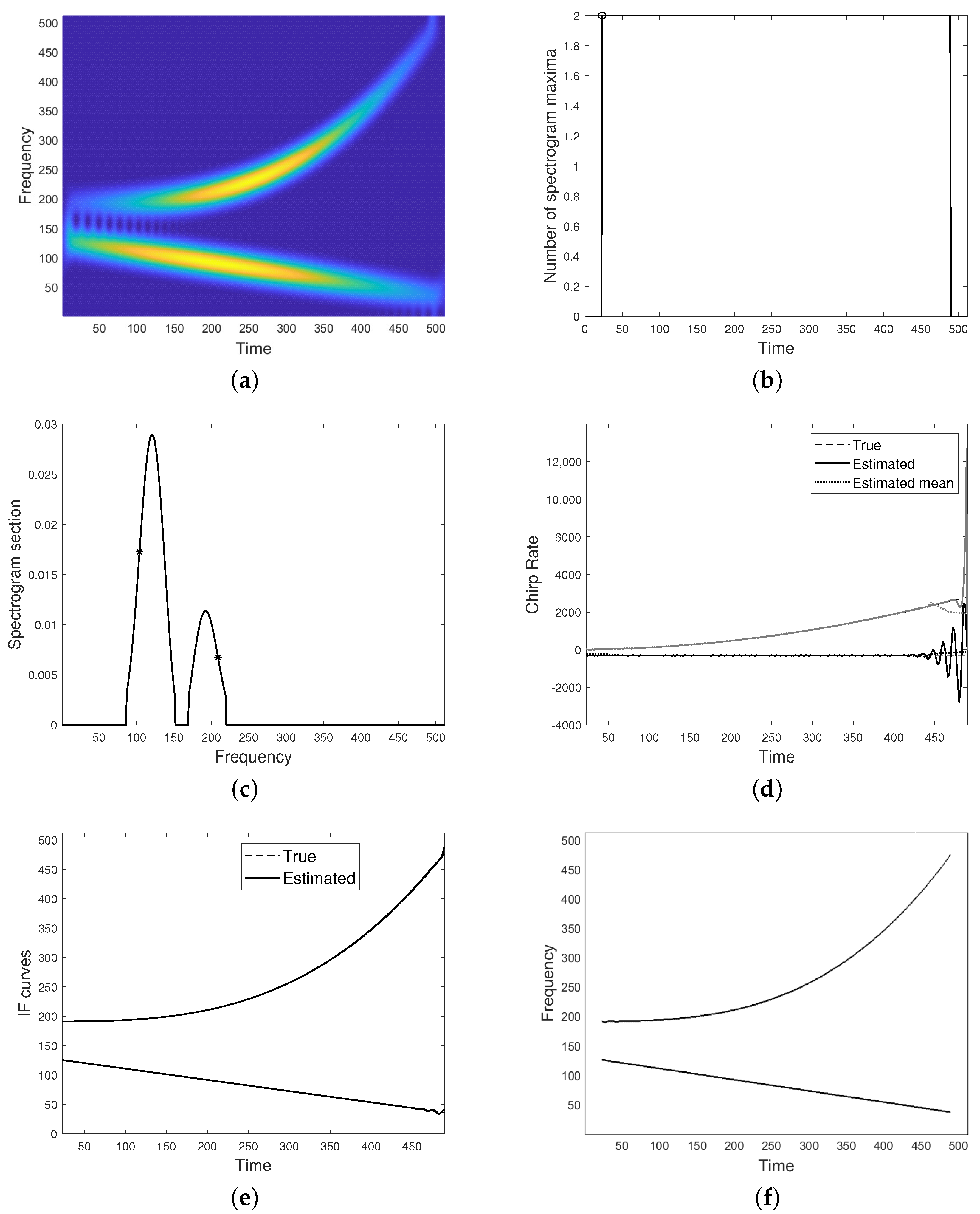
• The proposed model allows for IFs estimation, up to an integration constant, whose accuracy can affect the final result, as previously shown. However, it is worth pointing out that this error often causes the recovery of a characteristic different from the ridge, but still a characteristic. As a result, it contains significant information concerning IF. The integration constant can be directly estimated from spectrogram ridges belonging to the separability region. Also in this case, a prior TF localization of the non-separability region would solve the problem.
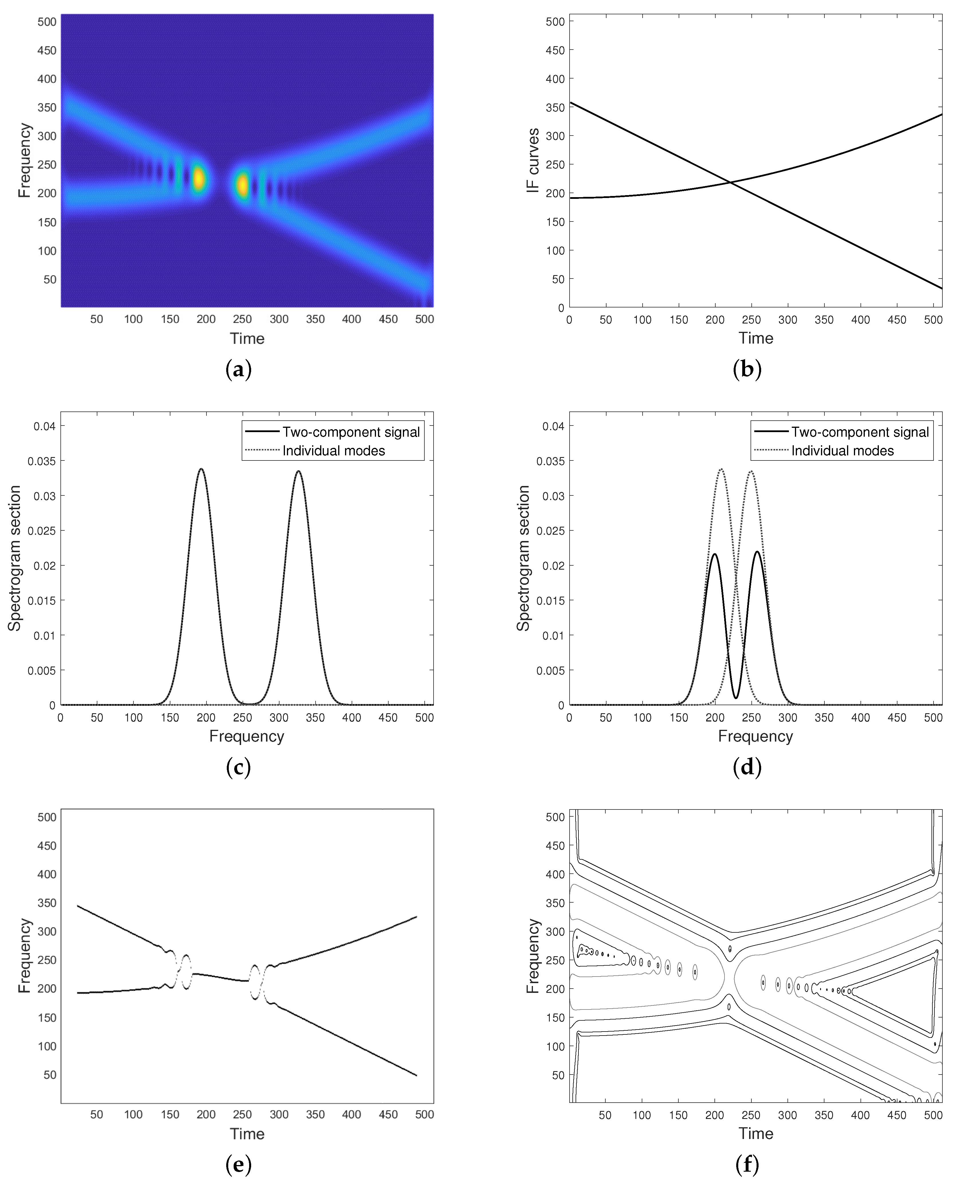
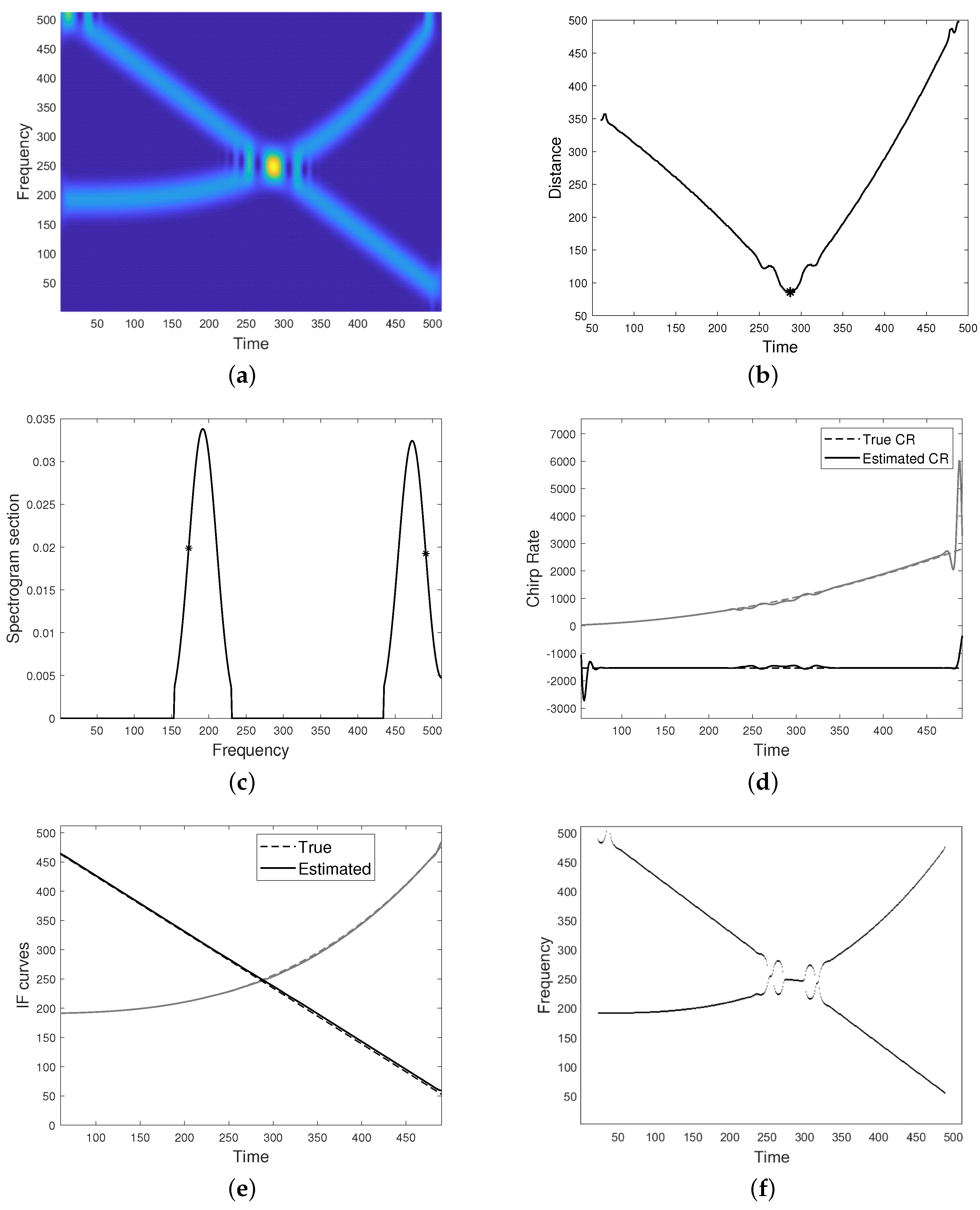
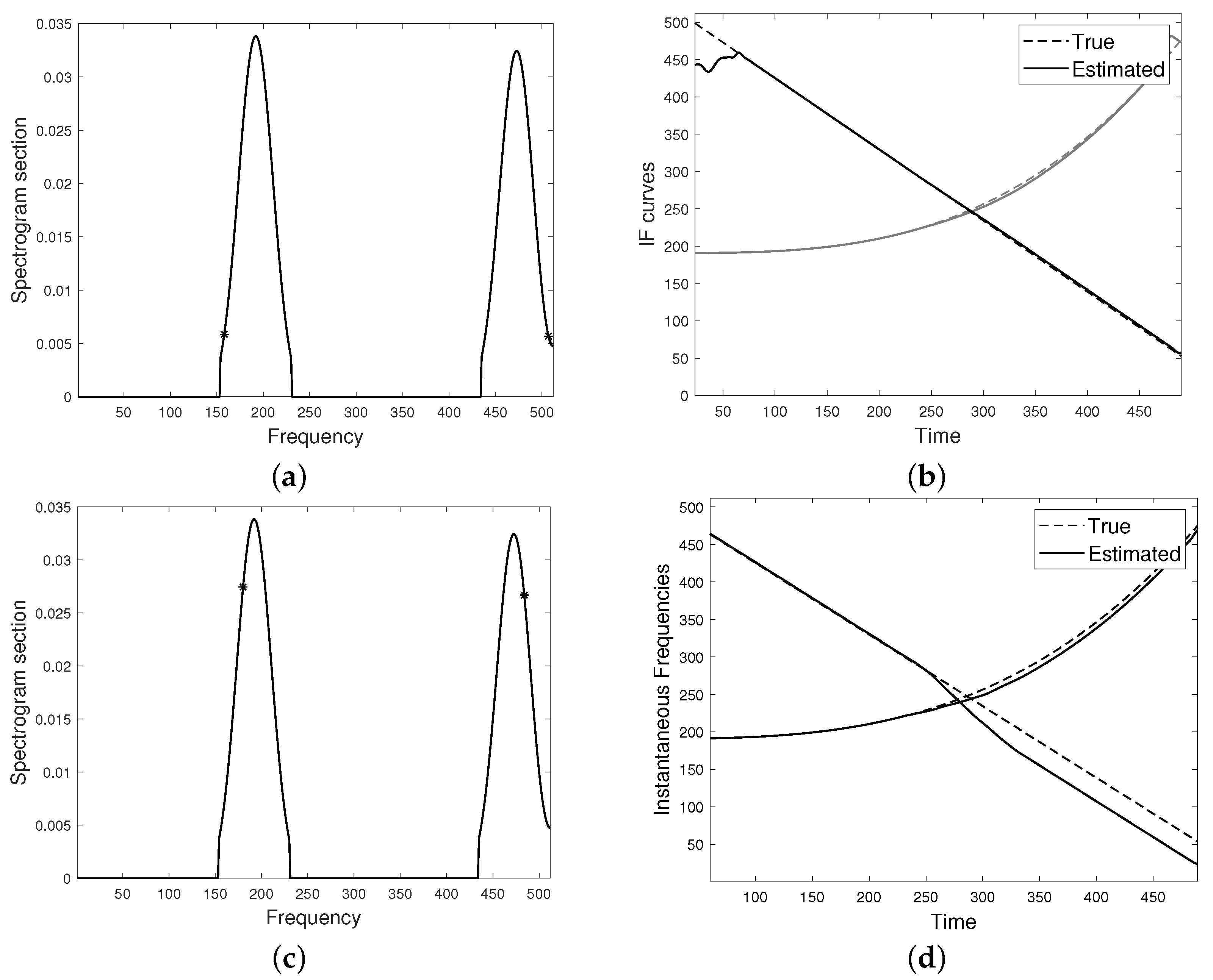
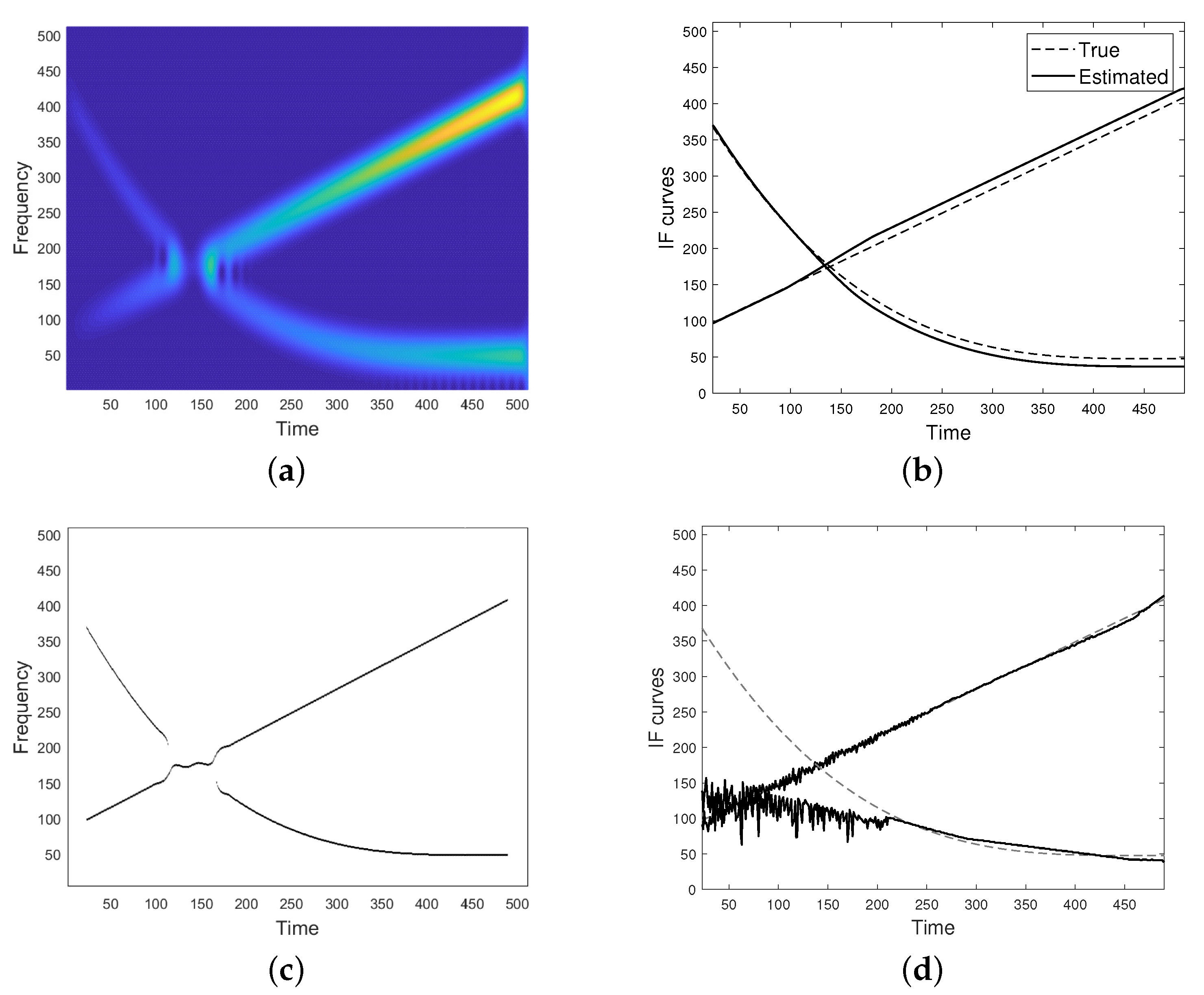
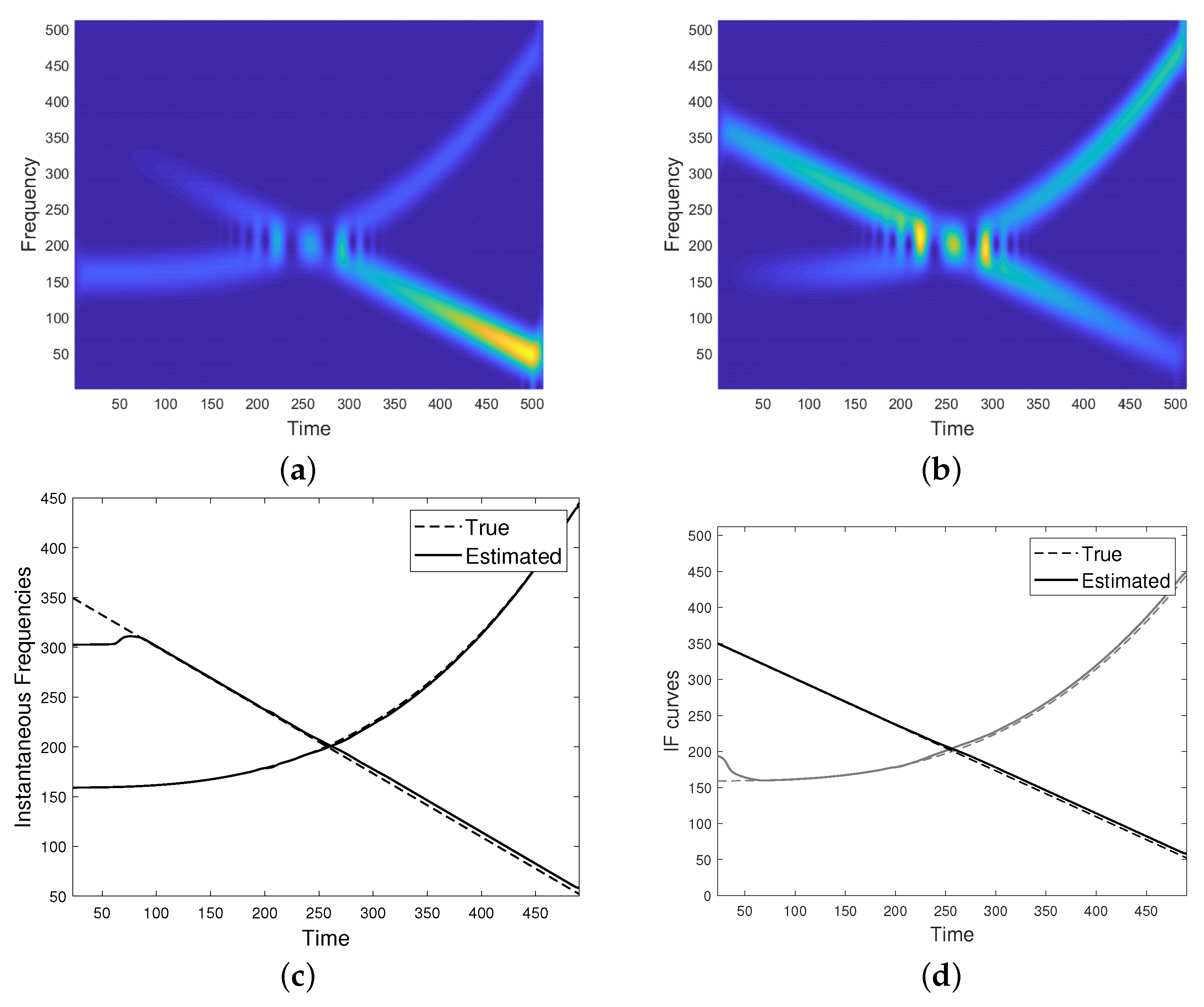
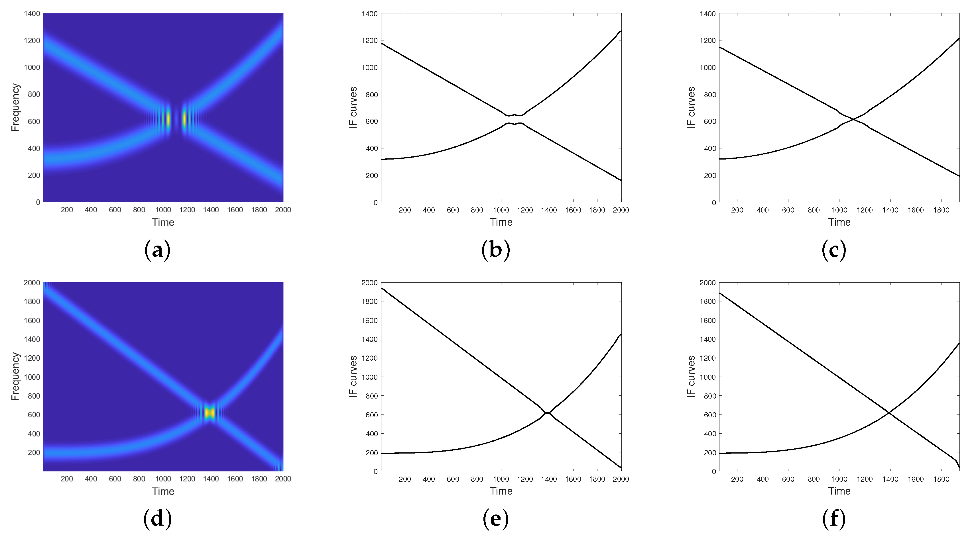
• The proposed procedure requires two frequency points for defining the linear system as in Equation (11), for each fixed u. The sensitivity to their selection has been numerically investigated. As shown in Figure 5 and Figure 6, involving too low characteristic curves can affect the final accuracy due to boundary effects, while characteristic at higher levels are generally more subjected to interference, resulting in inaccurate IFs estimate. For this reason, a good compromise can be achieved by selecting two frequency points close to the one where spectrogram concavity changes, as done in the presented simulations.
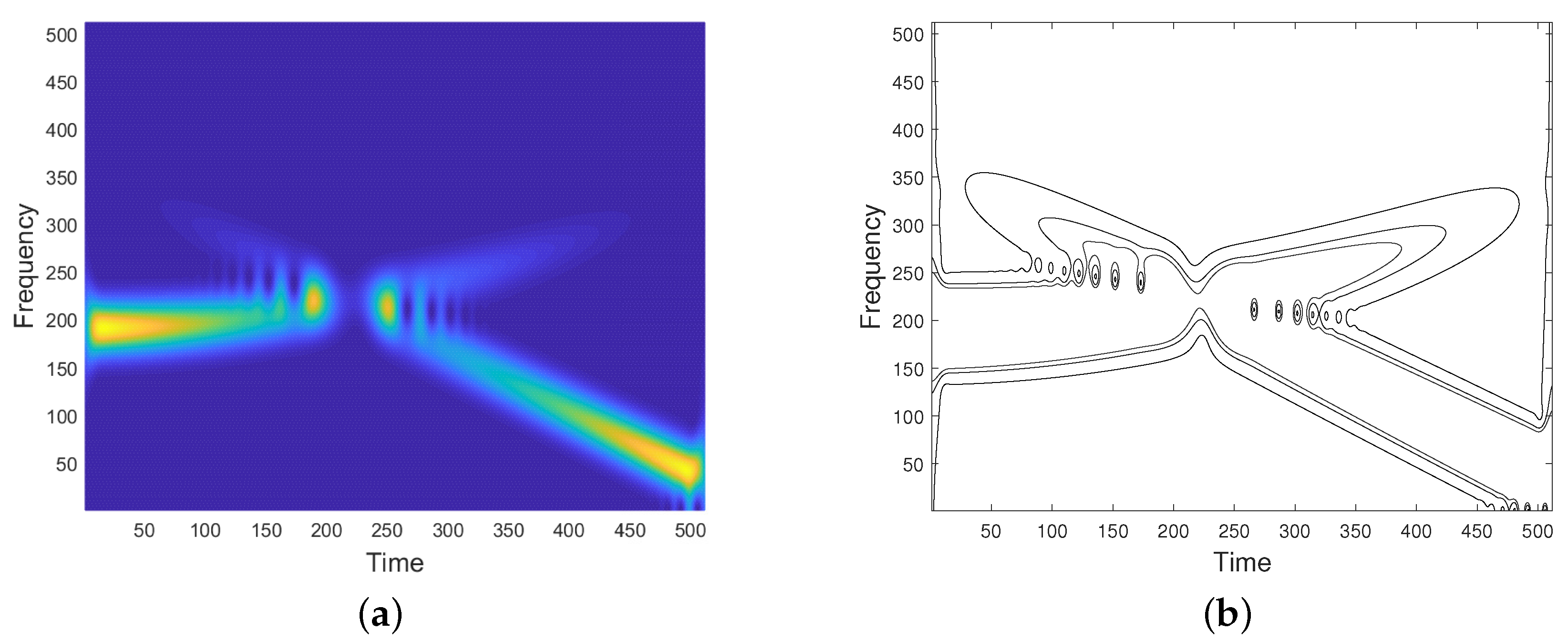
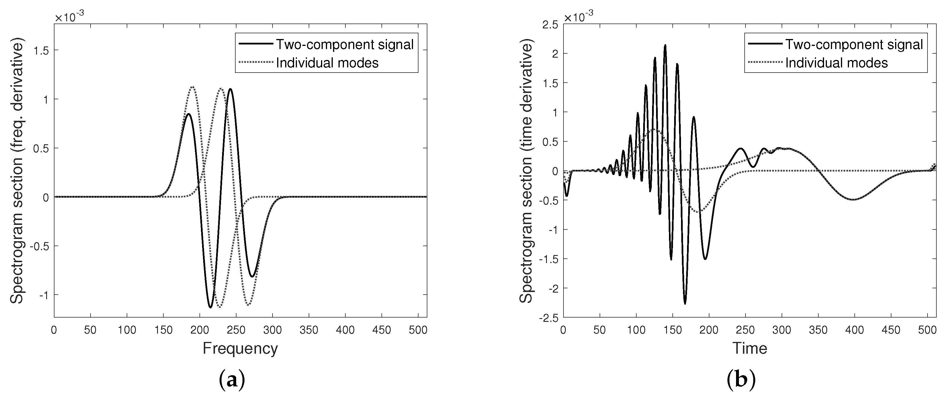
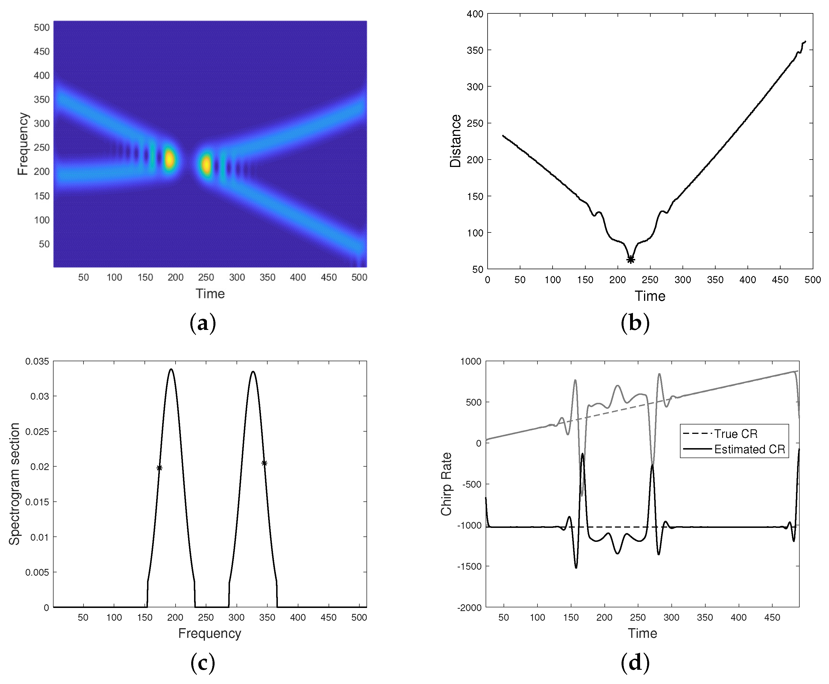
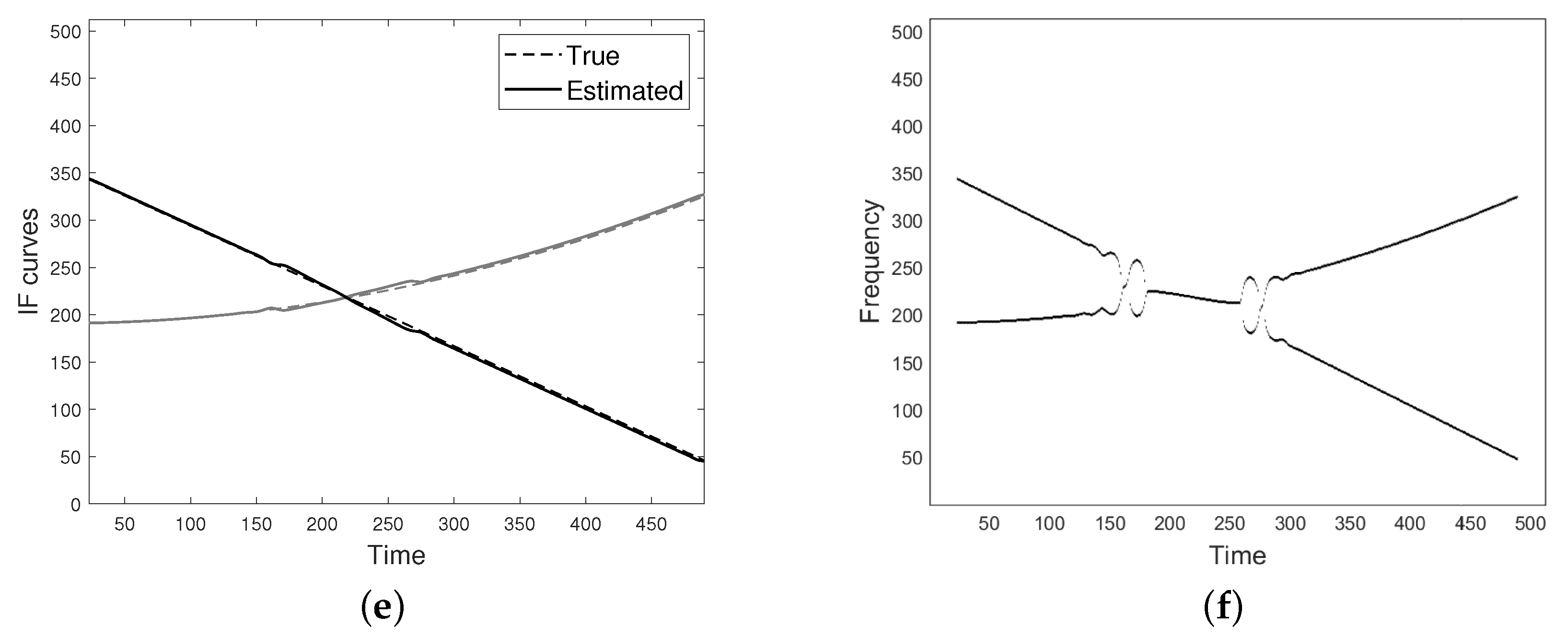
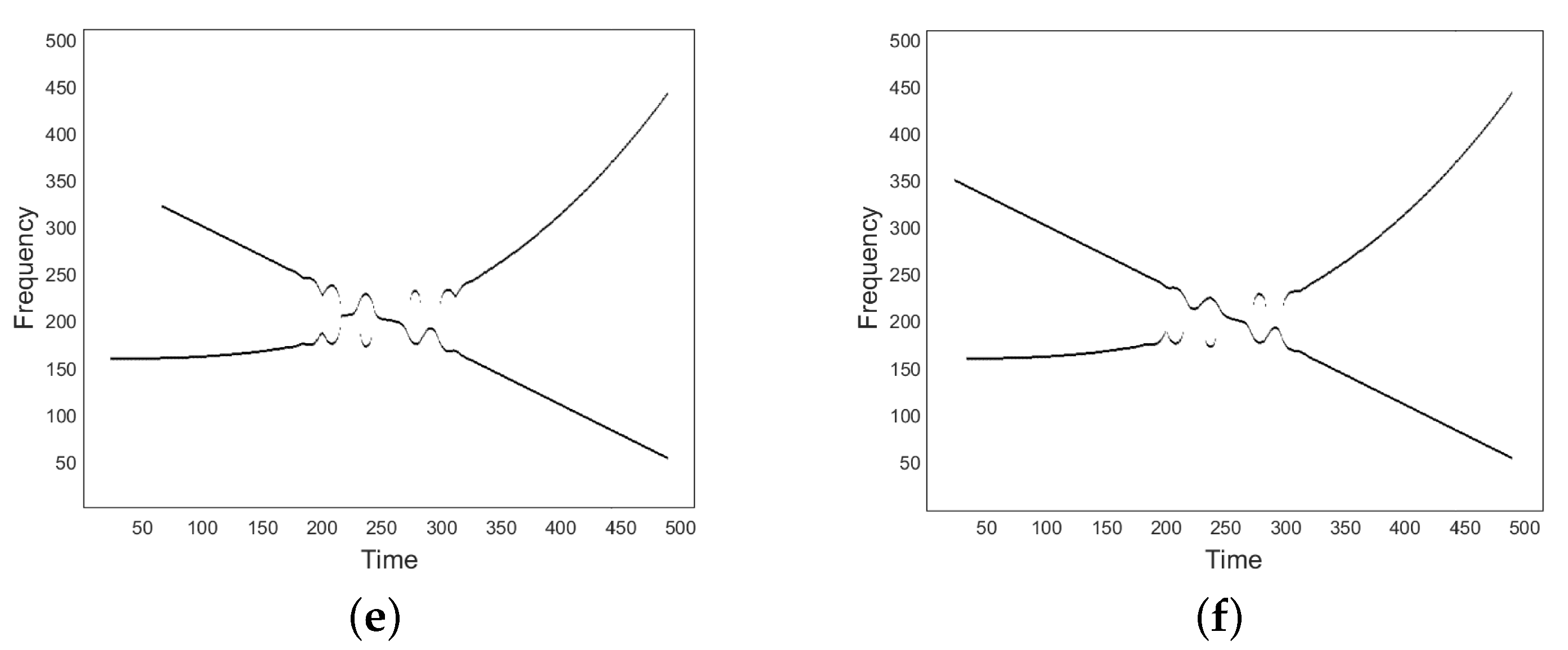
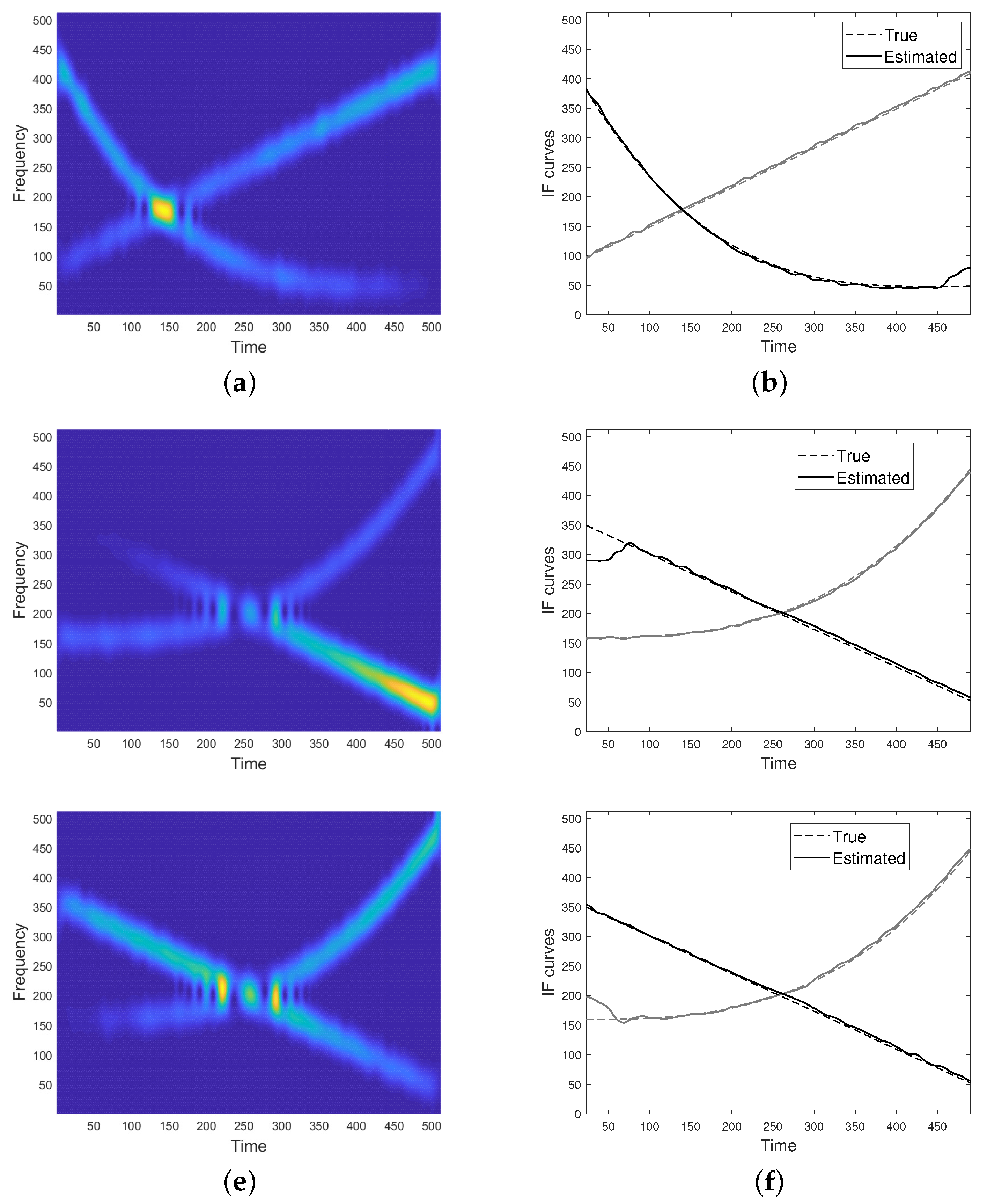
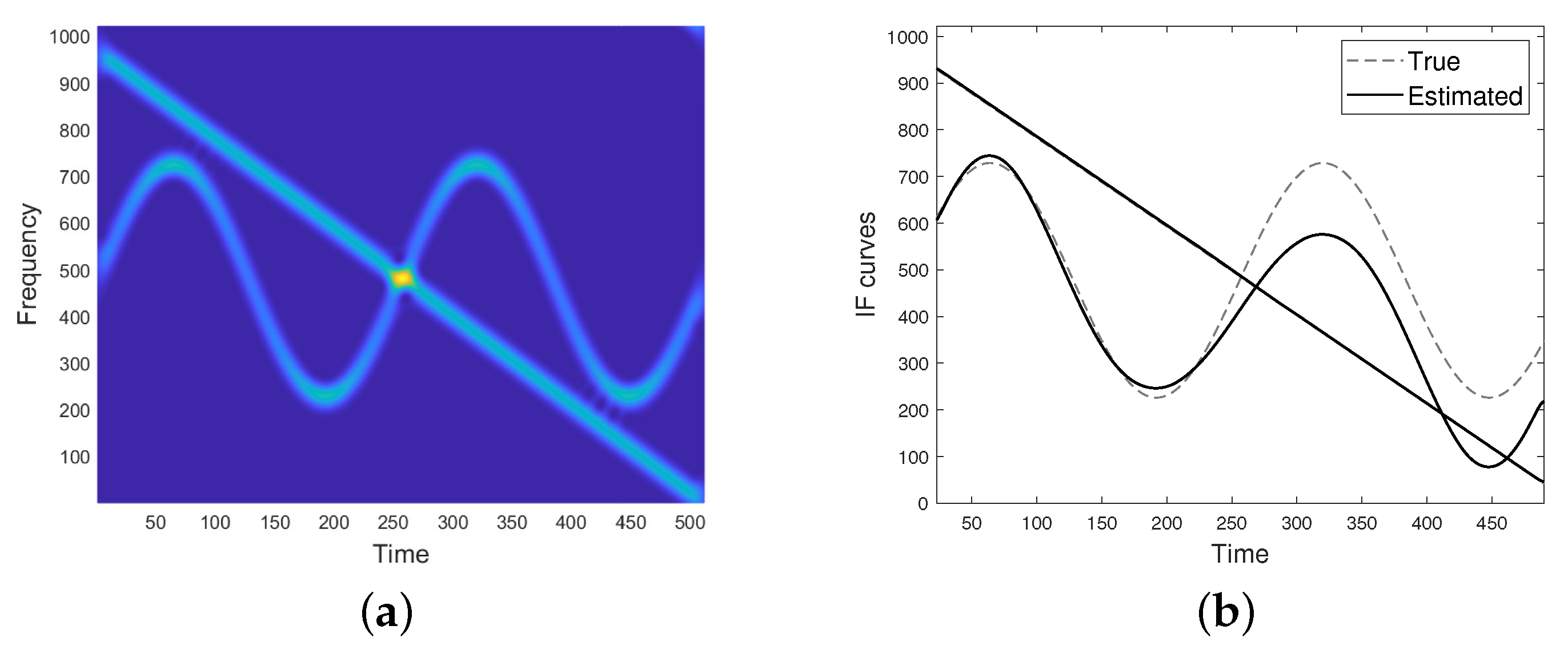
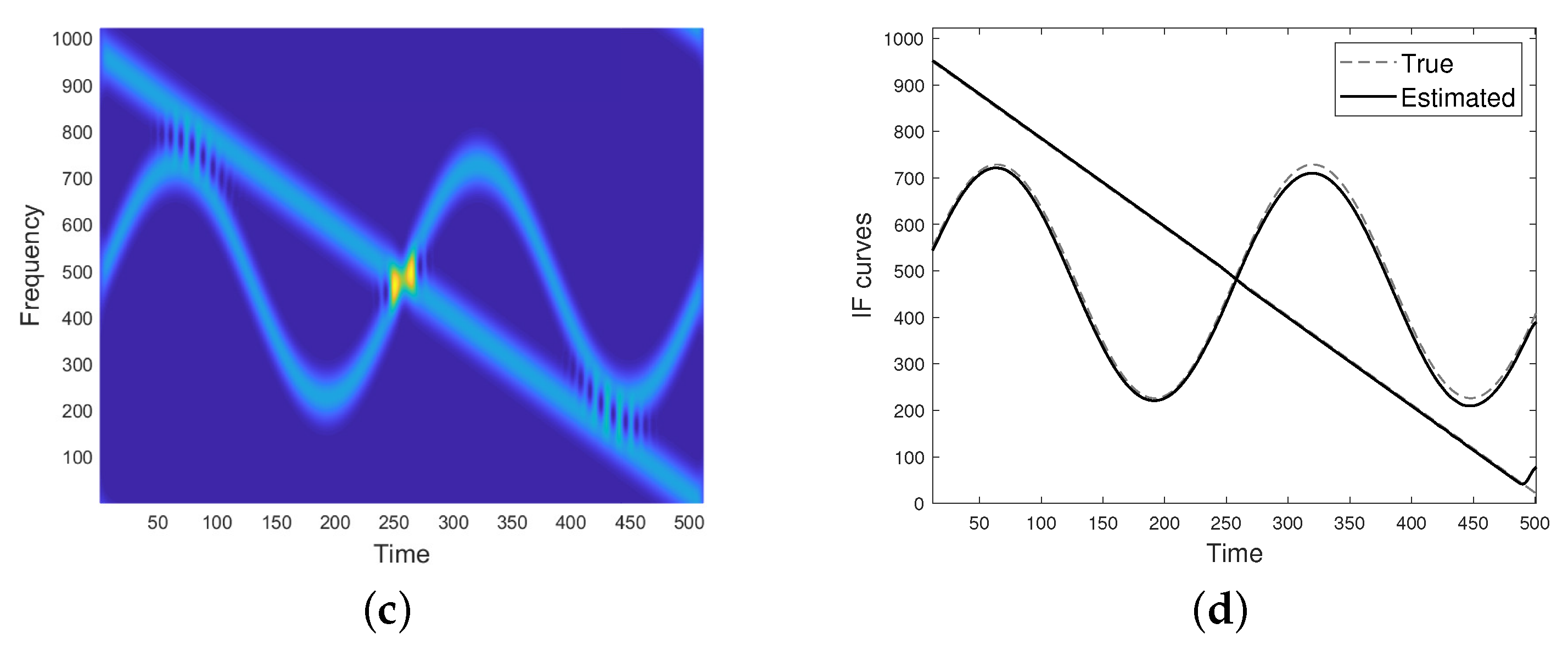
• As shown in the experimental results, the proposed method is robust to additive interference and cross-terms. The presence of spectrogram values close to zero, which occurs in case of strong amplitude modulation as well as destructive interference, could result in instabilities in the derivatives approximation, that can affect the final IFs estimation. However, it is worth highlighting that the proposed approach outperforms the state-of-the-art method in dealing with the critical case of destructive interference, as shown in Figure 7 and Figure 12. In addition, the proposed method has shown robustness to moderate noise.
• Spectrogram is widely used in practical applications because of its simplicity and computational benefit. It is well-known that, in case of MCS, spectrogram of close modes suffers from the presence of cross-terms that can affect each estimation concerning the signal. For this reason, more advanced and adaptive kernels with attenuated cross-terms, such as S-Transform or Locally Adaptive TF distribution, are often preferred in the literature. However, it is worth noticing that many real-life measurements, such as the ones concerning human gait classification and detection, precisely deal with spectrograms. That is why spectrogram processing is still of interest, today. In addition, cross-terms do not represent a limitation for the presented method, but a tool for estimating IF.

4. Conclusions

This paper has proposed a non-linear time-frequency evolution law for the spectrogram of a frequency and amplitude modulated two-component signal, which is employed for instantaneous frequencies (IFs) estimation. Based on the concept of weakened separability, the latter equation can be reduced to the one referred to a single mode, whose coefficients linearly depend on signal IFs time derivatives, namely the chirp rates (CRs). Approximating spectrogram derivatives and replacing them in the evolution law yields to a linear system with signals CRs as unknown variables. As a result, CRs can be detected by simply solving a two-dimensional linear system and IFs can be estimated by numerical integration. The experimental results presented in the paper have confirmed method effectiveness in dealing with amplitude modulated two-component signals with interfering modes. A comparative study with some of the state-of-the-art methods has been also provided, showing the benefits of the proposed method in processing modes affected by destructive interference.

IF curves estimation provided by the proposed method can be adopted as starting point for all variational methods dealing with interfering modes and requiring an initialization step. In addition, since it provides CRs estimation, the introduced procedure can be useful in reallocation techniques that involve high-order phase time derivatives.

As main advantage, the presented approach is non-parametric. However, IF law may be obtained by fixing the IF class and by interpolating the result provided by the proposed method.

As future developments, the method could be employed also for instantaneous amplitudes estimation. In addition, future studies will be aimed at defining an automatic procedure for interference region detection, in order to extend the proposed method to general multicomponent signals, having more than two modes. The applicability of the presented approach to time-frequency distributions different from the spectrogram will be also investigated.

References

- Chen, V.C.; Li, F.; Ho, S.S.; Wechsler, H. Micro-Doppler effect in radar: Phenomenon, model, and simulation study. IEEE Trans. Aerosp. Electron. Syst. 2006, 42, 2–21. [Google Scholar] [CrossRef]
- Lyonnet, B.; Ioana, C.; Amin, M.G. Human gait classification using microdoppler time-frequency signal representations. In Proceedings of the 2010 IEEE Radar Conference, Washington, DC, USA, 10–14 May 2010; pp. 915–919. [Google Scholar] [CrossRef]
- Zhang, Q.; Yeo, T.S.; Tan, H.S.; Luo, Y. Imaging of a Moving Target With Rotating Parts Based on the Hough Transform. IEEE Trans. Geosci. Remote Sens. 2008, 46, 291–299. [Google Scholar] [CrossRef]
- Shi, Y.; Zhang, D.; Ji, H.; Dai, R. Application of Synchrosqueezed Wavelet Transform in Microseismic Monitoring of Mines. In Proceedings of the 2019 IOP Conference Series: Earth and Environmental Science, Ho Chi Minh City, Vietnam, 25–28 February 2019; IOP Publishing: Bristol, UK, 2019; Volume 384, p. 012075. [Google Scholar] [CrossRef]
- Candes, E.J.; Charlton, P.R.; Helgason, H. Detecting highly oscillatory signals by chirplet path pursuit. Appl. Comput. Harmon. Anal. 2008, 24, 14–40. [Google Scholar] [CrossRef]
- Pham, D.H.; Meignen, S. High-order synchrosqueezing transform for multicomponent signals analysis with an application to gravitational-wave signal. IEEE Trans. Signal Process. 2017, 65, 3168–3178. [Google Scholar] [CrossRef]
- Guillemain, P.; Kronland-Martinet, R. Characterization of acoustic signals through continuous linear time-frequency representations. Proc. IEEE 1996, 84, 561–585. [Google Scholar] [CrossRef]
- Zeng, F.G.; Nie, K.; Stickney, G.S.; Kong, Y.Y.; Vongphoe, M.; Bhargave, A.; Wei, C.; Cao, K. Speech recognition with amplitude and frequency modulations. Proc. Natl. Acad. Sci. USA 2005, 102, 2293–2298. [Google Scholar] [CrossRef]
- Ioana, C.; Gervaise, C.; Stéphan, Y.; Mars, J.I. Analysis of underwater mammal vocalisations using time–frequency-phase tracker. Appl. Acoust. 2010, 71, 1070–1080. [Google Scholar] [CrossRef]
- Wang, G.; Teng, C.; Li, K.; Zhang, Z.; Yan, X. The removal of EOG artifacts from EEG signals using independent component analysis and multivariate empirical mode decomposition. IEEE J. Biomed. Health Inform. 2015, 20, 1301–1308. [Google Scholar] [CrossRef]
- Boashash, B. Time-Frequency Signal Analysis and Processing: A Comprehensive Reference; Academic Press: Cambridge, MA, USA, 2015. [Google Scholar]
- Huang, N.E.; Shen, Z.; Long, S.R.; Wu, M.C.; Shih, H.H.; Zheng, Q.; Yen, N.C.; Tung, C.C.; Liu, H.H. The empirical mode decomposition and the Hilbert spectrum for nonlinear and non-stationary time series analysis. Proc. R. Soc. Lond. Ser. Math. Phys. Eng. Sci. 1998, 454, 903–995. [Google Scholar] [CrossRef]
- Wu, Z.; Huang, N.E. Ensemble empirical mode decomposition: A noise-assisted data analysis method. Adv. Adapt. Data Anal. 2009, 1, 1–41. [Google Scholar] [CrossRef]
- Cicone, A. Nonstationary signal decomposition for dummies. In Advances in Mathematical Methods and High Performance Computing; Springer: Berlin/Heidelberg, Germany, 2019; pp. 69–82. [Google Scholar] [CrossRef]
- Dragomiretskiy, K.; Zosso, D. Variational mode decomposition. IEEE Trans. Signal Process. 2014, 62, 531–544. [Google Scholar] [CrossRef]
- Upadhyay, A.; Sharma, M.; Pachori, R.B.; Sharma, R. A Nonparametric Approach for Multicomponent AM–FM Signal Analysis. Circuits Syst. Signal Process. 2020, 39, 6316–6357. [Google Scholar] [CrossRef]
- Doweck, Y.; Amar, A.; Cohen, I. Joint model order selection and parameter estimation of chirps with harmonic components. IEEE Trans. Signal Process. 2015, 63, 1765–1778. [Google Scholar] [CrossRef]
- Yang, Y.; Dong, X.; Peng, Z.; Zhang, W.; Meng, G. Component extraction for non-stationary multi-component signal using parameterized de-chirping and band-pass filter. IEEE Signal Process. Lett. 2015, 22, 1373–1377. [Google Scholar] [CrossRef]
- Feng, Z.; Chu, F.; Zuo, M.J. Time–frequency analysis of time-varying modulated signals based on improved energy separation by iterative generalized demodulation. J. Sound Vib. 2011, 330, 1225–1243. [Google Scholar] [CrossRef]
- Stankovic, L. Analysis of noise in time-frequency distributions. IEEE Signal Process. Lett. 2002, 9, 286–289. [Google Scholar] [CrossRef]
- Stankovic, L.; Katkovnik, V. The Wigner distribution of noisy signals with adaptive time-frequency varying window. IEEE Trans. Signal Process. 1999, 47, 1099–1108. [Google Scholar] [CrossRef]
- Bouchikhi, A.; Boudraa, A.O.; Cexus, J.C.; Chonavel, T. Analysis of multicomponent LFM signals by Teager Huang-Hough transform. IEEE Trans. Aerosp. Electron. Syst. 2014, 50, 1222–1233. [Google Scholar] [CrossRef]
- Barbarossa, S. Analysis of multicomponent LFM signals by a combined Wigner-Hough transform. IEEE Trans. Signal Process. 1995, 43, 1511–1515. [Google Scholar] [CrossRef]
- Wood, J.C.; Barry, D.T. Radon transformation of time-frequency distributions for analysis of multicomponent signals. IEEE Trans. Signal Process. 1994, 42, 3166–3177. [Google Scholar] [CrossRef]
- Alieva, T.; Bastiaans, M.J.; Stankovic, L. Signal reconstruction from two close fractional Fourier power spectra. IEEE Trans. Signal Process. 2003, 51, 112–123. [Google Scholar] [CrossRef]
- Stankovic, L.; Dakovic, M.; Thayaparan, T.; Popovic-Bugarin, V. Inverse radon transform–based micro-Doppler analysis from a reduced set of observations. IEEE Trans. Aerosp. Electron. Syst. 2015, 51, 1155–1169. [Google Scholar] [CrossRef]
- Bruni, V.; Tartaglione, M.; Vitulano, D. Radon spectrogram-based approach for automatic IFs separation. EURASIP J. Adv. Signal Process. 2020, 13, 1–21. [Google Scholar] [CrossRef]
- Khan, N.A.; Boashash, B. Multi-component instantaneous frequency estimation using locally adaptive directional time frequency distributions. Int. J. Adapt. Control Signal Process. 2016, 30, 429–442. [Google Scholar] [CrossRef]
- Mohammadi, M.; Pouyan, A.A.; Khan, N.A.; Abolghasemi, V. Locally optimized adaptive directional time–frequency distributions. Circuits Syst. Signal Process. 2018, 37, 3154–3174. [Google Scholar] [CrossRef]
- Carmona, R.A.; Hwang, W.L.; Torresani, B. Characterization of signals by the ridges of their wavelet transform. IEEE Trans. Signal Process. 1997, 45, 2586–2590. [Google Scholar] [CrossRef]
- Carmona, R.; Hwang, W.; Torresani, B. Multiridge detection and time-frequency reconstruction. IEEE Trans. Signal Process. 1999, 47, 480–492. [Google Scholar] [CrossRef]
- Zhu, X.; Zhang, Z.; Gao, J.; Li, W. Two robust approaches to multicomponent signal reconstruction from STFT ridges. Mech. Syst. Signal Process. 2019, 115, 720–735. [Google Scholar] [CrossRef]
- Bruni, V.M.S.; Piccoli, B.; Vitulano, D. Instantaneous frequency detection via ridge neighbor tracking. In Proceedings of the 2010 2nd International Workshop on Cognitive Information Processing, Elba, Italy, 14–16 June 2010. [Google Scholar] [CrossRef]
- Rankine, L.; Mesbah, M.; Boashash, B. IF estimation for multicomponent signals using image processing techniques in the time–frequency domain. Signal Process. 2007, 87, 1234–1250. [Google Scholar] [CrossRef]
- Zhang, H.; Bi, G.; Yang, W.; Razul, S.G.; See, C.M.S. IF estimation of FM signals based on time-frequency image. IEEE Trans. Aerosp. Electron. Syst. 2015, 51, 326–343. [Google Scholar] [CrossRef]
- Stankovic, L.; Djurovic, I.; Ohsumi, A.; Ijima, H. Instantaneous frequency estimation by using Wigner distribution and Viterbi algorithm. In Proceedings of the 2003 IEEE International Conference on Acoustics, Speech, and Signal Processing, Hong Kong, China, 6–10 April 2003; Volume 6, pp. 6–121. [Google Scholar] [CrossRef]
- Djurović, I.; Stanković, L. An algorithm for the Wigner distribution based instantaneous frequency estimation in a high noise environment. Signal Process. 2004, 84, 631–643. [Google Scholar] [CrossRef]
- Khan, N.A.; Mohammadi, M.; Djurović, I. A Modified Viterbi Algorithm-Based IF Estimation Algorithm for Adaptive Directional Time–Frequency Distributions. Circuits Syst. Signal Process. 2019, 38, 2227–2244. [Google Scholar] [CrossRef]
- Li, P.; Zhang, Q.H. IF estimation of overlapped multicomponent signals based on Viterbi algorithm. Circuits Syst. Signal Process. 2020, 39, 3105–3124. [Google Scholar] [CrossRef]
- Li, P.; Zhang, Q.H. An improved Viterbi algorithm for IF extraction of multicomponent signals. Signal Image Video Process. 2018, 12, 171–179. [Google Scholar] [CrossRef]
- Khan, N.A.; Mohammadi, M.; Ali, S. Instantaneous frequency estimation of intersecting and close multi-component signals with varying amplitudes. Signal Image Video Process. 2019, 13, 517–524. [Google Scholar] [CrossRef]
- Chen, S.; Dong, X.; Xing, G.; Peng, Z.; Zhang, W.; Meng, G. Separation of overlapped non-stationary signals by ridge path regrouping and intrinsic chirp component decomposition. IEEE Sens. J. 2017, 5994–6005. [Google Scholar] [CrossRef]
- Dong, X.; Chen, S.; Xing, G.; Peng, Z.; Zhang, W.; Meng, G. Doppler Frequency Estimation by Parameterized Time-Frequency Transform and Phase Compensation Technique. IEEE Sens. J. 2018, 18, 3734–3744. [Google Scholar] [CrossRef]
- Chen, S.; Dong, X.; Peng, Z.; Zhang, W.; Meng, G. Nonlinear chirp mode decomposition: A variational method. IEEE Trans. Signal Process. 2017, 65, 6024–6037. [Google Scholar] [CrossRef]
- Bruni, V.; Marconi, S.; Piccoli, B.; Vitulano, D. Instantaneous frequency estimation of interfering FM signals through time-scale isolevel curves. Signal Process. 2013, 93, 882–896. [Google Scholar] [CrossRef]
- Stanković, L.; Mandić, D.; Daković, M.; Brajović, M. Time-frequency decomposition of multivariate multicomponent signals. Signal Process. 2018, 142, 468–479. [Google Scholar] [CrossRef]
- Ding, Y.; Tang, J. Micro-Doppler trajectory estimation of pedestrians using a continuous-wave radar. IEEE Trans. Geosci. Remote Sens. 2014, 52, 5807–5819. [Google Scholar] [CrossRef]
- Chen, S.; Yang, Y.; Wei, K.; Dong, X.; Peng, Z.; Zhang, W. Time-varying frequency-modulated component extraction based on parameterized demodulation and singular value decomposition. IEEE Trans. Instrum. Meas. 2015, 65, 276–285. [Google Scholar] [CrossRef]
- Yang, Y.; Peng, Z.; Dong, X.; Zhang, W.; Meng, G. Application of parameterized time-frequency analysis on multicomponent frequency modulated signals. IEEE Trans. Instrum. Meas. 2014, 63, 3169–3180. [Google Scholar] [CrossRef]
- Ioana, C.; Jarrot, A.; Gervaise, C.; Stéphan, Y.; Quinquis, A. Localization in underwater dispersive channels using the time-frequency-phase continuity of signals. IEEE Trans. Signal Process. 2010, 58, 4093–4107. [Google Scholar] [CrossRef]
- Chen, S.; Dong, X.; Yang, Y.; Zhang, W.; Peng, Z.; Meng, G. Chirplet path fusion for the analysis of time-varying frequency-modulated signals. IEEE Trans. Ind. Electron. 2016, 64, 1370–1380. [Google Scholar] [CrossRef]
- Swärd, J.; Brynolfsson, J.; Jakobsson, A.; Hansson-Sandsten, M. Sparse semi-parametric estimation of harmonic chirp signals. IEEE Trans. Signal Process. 2015, 64, 1798–1807. [Google Scholar] [CrossRef]
- Djurović, I.; Simeunović, M.; Wang, P. Cubic phase function: A simple solution to polynomial phase signal analysis. Signal Process. 2017, 135, 48–66. [Google Scholar] [CrossRef]
- Zhu, X.; Zhang, Z.; Zhang, H.; Gao, J.; Li, B. Generalized Ridge Reconstruction Approaches Toward more Accurate Signal Estimate. Circuits Syst. Signal Process. 2019, 1–26. [Google Scholar] [CrossRef]
- Auger, F.; Flandrin, P.; Lin, Y.-T.; McLaughlin, S.; Meignen, S.; Oberlin, T.; Wu, H.-T. Time-Frequency reassignment and synchrosqueezing: An overview. IEEE Signal Process. Mag. 2013, 30, 32–41. [Google Scholar] [CrossRef]
- Daubechies, I.; Lu, J.; Wu, H.T. Synchrosqueezed wavelet transforms: An empirical mode decomposition-like tool. Appl. Comput. Harmon. Anal. 2011, 30, 243–261. [Google Scholar] [CrossRef]
- Daubechies, I.; Wang, Y.; Wu, H. ConceFT: Concentration of frequency and time via a multitapered synchrosqueezed transform. Philos. Trans. R. Soc. A Math. Phys. Eng. Sci. 2015, 374, 20150193. [Google Scholar] [CrossRef] [PubMed]
- Yu, G.; Yu, M.; Xu, C. Synchroextracting transform. IEEE Trans. Aerosp. Electron. Syst. 2017, 64, 8042–8054. [Google Scholar] [CrossRef]
- Zhu, X.; Yang, H.; Zhang, Z.; Gao, J.; Liu, N. Frequency-chirprate reassignment. Digit. Signal Process. 2020, 102783. [Google Scholar] [CrossRef]
- Bruni, V.; Tartaglione, M.; Vitulano, D. A fast and robust spectrogram reassignment method. Mathematics 2019, 7, 358. [Google Scholar] [CrossRef]
- Bruni, V.; Tartaglione, M.; Vitulano, D. An iterative approach for spectrogram reassignment of frequency modulated multicomponent signals. Math. Comput. Simul. 2020, 176, 96–119. [Google Scholar] [CrossRef]
- Mallat, S. A Wavelet Tour of Signal Processing; Elsevier: Amsterdam, The Netherlands, 1999. [Google Scholar]
- Bruni, V.; Tartaglione, M.; Vitulano, D. A Signal Complexity-Based Approach for AM–FM Signal Modes Counting. Mathematics 2020, 8, 2170. [Google Scholar] [CrossRef]
- Variational Nonlinear Chirp Mode Decomposition. Available online: https://www.mathworks.com/matlabcentral/fileexchange/64292-variational-nonlinear-chirp-mode-decomposition (accessed on 2 December 2020).
- Bruni, V.; Della Cioppa, L.; Vitulano, D. A Multiscale Energy-Based Time-Domain Approach for Interference Detection in Non-stationary Signals. In International Conference on Image Analysis and Recognition; Springer: Berlin/Heidelberg Germany, 2020; pp. 36–47. [Google Scholar] [CrossRef]
Publisher’s Note: MDPI stays neutral with regard to jurisdictional claims in published maps and institutional affiliations. |
© 2021 by the authors. Licensee MDPI, Basel, Switzerland. This article is an open access article distributed under the terms and conditions of the Creative Commons Attribution (CC BY) license (http://creativecommons.org/licenses/by/4.0/).