On Spectral Decomposition of States and Gramians of Bilinear Dynamical Systems

Abstract

The article proves that the state of a bilinear control system can be split uniquely into generalized modes corresponding to the eigenvalues of the dynamics matrix. It is also shown that the Gramians of controllability and observability of a bilinear system can be divided into parts (sub-Gramians) that characterize the measure of these generalized modes and their interactions. Furthermore, the properties of sub-Gramians were investigated in relation to modal controllability and observability. We also propose an algorithm for computing the Gramians and sub-Gramians based on the element-wise computation of the solution matrix. Based on the proposed algorithm, a novel criterion for the existence of solutions to the generalized Lyapunov equation is proposed, which allows, in some cases, to expand the domain of guaranteed existence of a solution of bilinear equations. Examples are provided that illustrate the application and practical use of the considered spectral decompositions.

1. Introduction

Monitoring the state of various technical, social, and biological systems using non-linear mathematical models and modern information technology is a widely relied upon trend in the development of modern civilization. An example is the state estimation and control in modern electric power systems. Renewable energy sources and distributed generation, electric vehicles and charging networks, and the increased use of power electronics pose new challenges for the monitoring and controling of complex oscillations in energy systems [1]. New problems require the development of new methods for the analysis of non-linear dynamic systems, including computational methods for their solutions.

Bilinear control systems represent an important class of non-linear systems, which are linear in inputs and states, but they are not linear in both. Research in the field of non-linear and “weakly non-linear” control systems described by the Volterra series dates back more than half a century. In [2], a theory of realization was developed, and structural decompositions of the Gramians of bilinear systems were investigated; furthermore, explicit representations of the Gramian of a bilinear system were obtained in the form of a Volterra series, and the conditions for its convergence were investigated. In [3,4], the multivariate Laplace transform was used to construct a solution for systems with smooth non-linearities. In [5], an iterative solution of the generalized Lyapunov equation was obtained, which was first used to analyze the state of an electric power system. It was shown that a solution to this equation exists if the linear part of the bilinear system is stable, and the input signal and non-linearity matrices are bounded in the norm. In [6], these results were generalized for multiple-input and multiple-output (MIMO) dynamical systems.

Research in the field of bilinear control systems is closely related to the problem of model order reduction (MOR) by constructing an approximating model of a lower dimension. Among the methods for solving this problem, we note balanced truncation, singular decomposition, the Krylov subspace method, optimal methods for the $H_2$-norm of Gramians, and hybrid methods. For most of the methods, iterative algorithms for their implementation have been developed, and conditions for the existence and uniqueness of the solution of the corresponding generalized Lyapunov equations have been established [6,7,8,9]. In these studies, the squared $H_2$-norm of Gramians of the bilinear system was used, and its spectral expansions using singular values were obtained. To estimate the error between the full and reduced models, energy functionals were introduced, and the corresponding $H_2$-norm optimal algorithms for the interpolation of bilinear systems were proposed.

Modal analysis and selective modal analysis are among the main methods for analyzing the stability of electric power systems with small deviations from the steady state. These methods involve identifying dominant weakly stable modes of the power system and are widely used in combination with other linear and non-linear analysis methods [1,10]. To assess bilinear effects in power systems analysis, the technique of normal forms [11], modal series methods [12], and bilinear approximation [13] are used. These methods consider the higher-order terms of the Taylor expansion in the system approximation and use normal Poincaré forms. In [14], a method was proposed for the fast computation of normal forms, considering the interaction of dominant modes. Ref. [15] proposes a hybrid method combining selective modal analysis and Koopman mode decomposition.

In contrast to these methods, in this study, we consider the spectral decomposition, not for the instantaneous dynamics of state variables, but for the Lyapunov functions, which characterize the $L_2$-norms of variables or signals in the time domain. This approach allows us to consider the non-linear effects associated with the accumulation of influence over time. For linear dynamic systems, Lyapunov functions are usually associated with the controllability and observability Gramians, which characterize the integrated energy of the input and output signals. The concept of Gramians was further generalized and interpreted for deterministic bilinear systems using energy functionals [16]. For linear systems, ref. [7] obtained singular expansions for infinite Gramians of controllability and observability based on the diagonalization of the dynamics matrix. A more general form of the spectral decomposition of Gramians into components (sub-Gramians) corresponding to the individual eigenvalues of the system or their pairwise combinations was proposed in [17,18]. In [19], the spectral expansions for the Gramians of controllability and observability were generalized to the case of bilinear continuous systems.

The purpose of this study is to develop and provide a rationale for the application of the spectral expansions of the Gramians proposed in [19] for the analysis and monitoring of bilinear systems. As the state of a bilinear system is not the sum of eigenmodes as in the linear case, a number of important theoretical questions arise. How should eigenmodes be viewed and interpreted in a bilinear system? What interpretation can be given to the spectral expansions of the Gramians in [19]? What is their connection with the expansion of the Gramians in linear systems?

Main Contribution

As spectral expansions of states of bilinear systems are closely related to the corresponding expansions of states of linear systems, in Section 2, we first consider the concepts of modal controllability and observability for a linear dynamical system. The following new results were obtained: Criteria for modal controllability and observability are proposed (Propositions 3 and 5), and a relation is established between the eigenmodes of the linear system and sub-Gramians of controllability and observability (Propositions 7 and 9).

The main theoretical results are presented in Section 3. We show that the solution of a bilinear system under any control can be split uniquely into generalized modes corresponding to the eigenvalues of the dynamics matrix (Proposition 11). The definitions of sub-Gramians are proposed in a new form, and their relationship with the definitions in [19] are clarified (Property 4). The conditions for the existence of sub-Gramians (Property 1) and their consistency with the concept of sub-Gramians in linear theory (Property 3) are established.

In [19], expressions for sub-Gramians were proposed in the form of solutions to the modal Lyapunov equations. In this study, the same quantities are derived as the sums of squared convolution kernels arising in the Volterra series expansion of the state of the bilinear system. Moreover, it is proved (in Property 4) that if these quantities exist, then for a stable matrix of dynamics, they coincide with the definition in [19]. Although the new definition of sub-Gramians essentially coincides with the definition in [19], it allows us to establish a relation between sub-Gramians and the corresponding generalized modes of a bilinear system, namely, to prove that sub-Gramians characterize some measure of the corresponding generalized eigenmodes and their pairwise scalar products (Proposition 5) under the condition that controls are small enough. From a theoretical point of view, this result provides a conceptual justification for the concept of sub-Gramians for bilinear systems. From the point of view of applications, it allows one to make energy-based estimates of individual generalized modes and their pairwise interactions in the system. Such estimates, in turn, can become the basis for stability analysis and optimal control in bilinear dynamical systems.

Section 4 proposes an iterative algorithm for computing the Gramians and sub-Gramians based on the element-wise computation of the solution matrix on an eigenvector basis. This algorithm is similar to the algorithms in [20]. However, based on the proposed algorithm, a novel criterion for the existence of solutions to the generalized Lyapunov equation is formulated (Theorem 4), which, in some cases, allows the expansion of the domain of guaranteed existence of a solution of bilinear equations. At the end of Section 4, some examples that illustrate the application and practical use of the considered spectral decompositions are presented.

2. Spectral Expansions of Gramians of Linear Systems

2.1. Eigenmode Decompositions of the Dynamics of a Linear System

In this section, we consider the eigen-decomposition of the dynamics of a linear stationary system, which will be required for further presentation. Consider a linear dynamical system of the form

$$\left\{\begin{array}{c}\dot{x}=Ax+Bu\\ y=Cx\end{array}\right.,$$

(1)

where $x\in {\mathbb{R}}^n$ is the state vector, and $y\in {\mathbb{R}}^l,u\in {\mathbb{R}}^m$ are the output signal and control, respectively. $A,B,C$ are real matrices. Suppose that the dynamics matrix A has a simple spectrum $\sigma \left(A\right)=\{{\lambda }_1,{\lambda }_2,\cdots ,{\lambda }_n\}$.

Proposition 1.

A matrix A with a simple spectrum can be represented as

$$A={\lambda }_1{R}_1+{\lambda }_2{R}_2+\cdots +{\lambda }_n{R}_n,$$

(2)

where$R_i$are the matrices of residues in the decomposition of the resolvent of matrix A:

$${\left(Is-A\right)}^{-1}=\frac{R_1}{s-{\lambda }_1}+\frac{R_2}{s-{\lambda }_2}+\cdots +\frac{R_n}{s-{\lambda }_n}.$$

(3)

Proof. 

When all eigenvalues are distinct, the residue matrices of the resolvent of matrix A can be calculated using the normalized right and left eigenvectors as $R_i=u_i{v}_i^T$ (see [21]). Then, representation (2) directly follows from the eigen decomposition of matrix A. □

From the representation of the residue matrices through the eigenvectors and the orthogonality of the eigenvectors, it follows that the residue matrices $R_i$ satisfy the following the orthogonality property:

$$R_i{R}_j=R_i{\delta }_{ij},$$

(4)

where ${\delta }_{ij}$ is the Kronecker delta. Thus, representation (2) of matrix A is $\mathit{separable}$ in the sense that all terms in it are orthogonal to each other in accordance with (4). If the matrices $R_i$ of residues are known, then using (2)–(4), one can easily find all the powers of the matrix A

$$A^k=\sum _i{\lambda }_i^k{R}_i,k=0,\pm 1,\pm 2,\cdots ,$$

(5)

and the summation index here and in the following are assumed to be from one to n. Substituting (5) into the Taylor expansion of the matrix exponent of A, we obtain

$$e^{At}=\sum _i{R}_i{e}^{{\lambda }_{i}t}.$$

(6)

Proposition 2

(Eigenmode decomposition). Solution, control, and output signal of linear system (1) are separable with respect to the eigenmodes, i.e., there is a representation

$$\begin{array}{c}x\left(t\right)=\sum _i{x}_i\left(t\right),u\left(t\right)=\sum _i{u}_i\left(t\right),y\left(t\right)=\sum _i{y}_i\left(t\right),\mathit{where}\\ x_i\left(t\right)=R_{i}x\left(t\right)=R_i{e}^{{\lambda }_{i}t}{x}_0+B{e}^{{\lambda }_{i}t}\underset{t_0}{\overset{t}{\int }}{e}^{-{\lambda }_i\tau }{u}_i\left(\tau \right)d\tau ,\\ u_i\left(t\right)=B^{\#}{R}_{i}Bu\left(t\right),y_i\left(t\right)=C{x}_i\left(t\right)=C{R}_{i}x\left(t\right),\end{array}$$

(7)

$x_0=x\left(t_0\right)$ is the initial position of the system, and $B^{\#}$ denotes the Moore–Penrose inverse. The system (1) splits into separate subsystems

$$\left\{\begin{array}{c}{\dot{x}}_i\left(t\right)={\lambda }_i{x}_i\left(t\right)+B{u}_i\left(t\right)\\ y_i\left(t\right)=C{x}_i\left(t\right)\end{array}\right.,i=1,\cdots ,n.$$

(8)

Recall that the Moore–Penrose inverse matrix $B^{\#}$ exists and is unique for any complex or real matrix B and it is defined by four conditions: (i) $B{B}^{\#}B=B$, (ii) $B^{\#}B{B}^{\#}=B^{\#}$, (iii) $B{B}^{\#}$ is Hermitian, and (iv) $B^{\#}B$ is Hermitian.

Proof. 

The expression (7) for $x_i\left(t\right)=R_{i}x\left(t\right)$ is obtained by multiplying the solution to (1):

$$x\left(t\right)=e^{At}{x}_0+e^{At}{\int }_{t_0}^t{e}^{-A\tau }Bu\left(\tau \right)d\tau$$

on the left by $R_i$, taking into account property (4) and also that $R_i{e}^{At}=R_i{e}^{{\lambda }_{i}t},e^{-A\tau }={\sum }_j{R}_j{e}^{-{\lambda }_j\tau },B{u}_i\left(\tau \right)=R_{i}Bu\left(\tau \right)$. If we differentiate (7), we obtain (8). □

The expression (7) for $x_i\left(t\right)=R_{i}x\left(t\right)$ determines the dynamics of the eigenmode corresponding to the eigenvalue ${\lambda }_i$ in system (1). The corresponding mode in the output signal is determined by the expression $y_i\left(t\right)=C{x}_i\left(t\right)$.

2.2. Modal Observability and Controllability of a Linear System

In this section, by analogy with the classical definitions of an observable and controllable linear system, we introduce the corresponding concepts for individual eigenmodes. We also establish simple criteria for modal controllability and observability for a linear stationary system (1).

Definition 1.

The mode corresponding to the eigenvalue ${\lambda }_i$ isobservablein the linear system (1) at the moment $t_0$, when $y_i(t,t_0,x_0,u=0)\equiv 0$ at $t\ge t_0$ if, and only if, $x_i\left(t_0\right)=0$.

According to (7), the observability of a mode in a stationary system (1) is entirely determined by the matrices $R_i$ and C. Therefore, we can also discuss the modal observability of a pair $\{C,R_i\}$. For stationary systems, modal observability can be verified using the following simple criterion.

Proposition 3.

The mode corresponding to ${\lambda }_i$ in the linear system (1) is observable. if, and only if, $C{R}_i\ne 0$.

Proof. 

If the stationary pair $\{C,R_i\}$ is modally observable, then $C{R}_i{x}_0\ne 0$ holds for any $R_i{x}_0\ne 0$, that is, for some $x_0\ne 0$, $C{R}_i{x}_0\ne 0$ is fulfilled, and therefore $C{R}_i\ne 0$. If $C{R}_i\ne 0$, then there is some $x_0\ne 0$ such that $C{R}_i{x}_0\ne 0$. Let us now choose an arbitrary $R_i{\tilde{x}}_0\ne 0$. It is easy to show that the vectors $R_i{x}_0$ and $R_i{\tilde{x}}_0$ are both eigenvectors of matrix A corresponding to the eigenvalue ${\lambda }_i$. Because, by assumption, the spectrum of $\sigma \left(A\right)$ is simple, these vectors are proportional, that is, $R_i{\tilde{x}}_0=\alpha R_i{x}_0,\alpha \in \mathbb{C}$. Therefore, $C{R}_i{\tilde{x}}_0=\alpha C{R}_i{x}_0\ne 0$, that is, the pair $\{C,R_i\}$ is modally observable. □

One can check the observability of the system by checking the observability of its individual modes.

Proposition 4.

The stationary system (1) is observable (identifiable) if, and only if, each mode is observable (identifiable).

Proof. 

It follows from the definitions and equivalence of the following statements

$$\forall i:y_i(t,t_0,x_0,u=0)\equiv 0\mathrm{at}t\ge t_0<=>y\left(t,t_0,x_0,u=0\right)\equiv 0\mathrm{at}t\ge t_0;$$

$$\forall i:x_i\left(t_0\right)=0<=>x\left(t_0\right)=0.\square$$

However, individual modes can be observable when the dynamical system (1) as a whole is unobservable.

Similarly, one can consider the concept of modal controllability and obtain a criterion for modal controllability.

Definition 2.

The mode corresponding to the eigenvalue ${\lambda }_i$ in the linear system (1)is controllable, if for each event $(t_0,x_0=x_i\left(t_0\right))$, there is a control $u\left(t\right)$, which brings the system to the zero state in a finite time.

For stationary systems, modal controllability can be verified using the following simple criterion.

Proposition 5.

The mode corresponding to ${\lambda }_i$ in the linear system (1) is controllable if, and only if, $R_{i}B\ne 0$.

Proof. 

If $R_{i}B=0$, then it follows from (7) that mode $x_i\left(t\right)$ is not controllable. If $R_{i}B\ne 0$, then $u\left(t\right)$ can always be chosen, such that

$${\int }_{t_0}^{t_0+T}{e}^{-{\lambda }_j\tau }u\left(\tau \right)d\tau =\left\{\begin{array}{c}{u}_i^0,j=i\\ 0,j\ne i\end{array}\right.,R_i{x}_0=-R_{i}B{u}_i^0,j=1,\dots ,n$$

Then, in a finite time T, the control $u\left(t\right)$ brings the system from state $x_i\left(t_0\right)=R_i{x}_0$ to the zero state, i.e., the eigen-mode corresponding to ${\lambda }_i$ is controllable. □

According to Proposition 5, the controllability of a mode in a stationary system is entirely determined by the matrices $R_i$ and B. Thus, we can discuss the modal controllability of the stationary pair$\{R_i,B\}$. The controllability of the system can be verified by checking the controllability of its individual modes.

Proposition 6.

A stationary linear system (1) is controllable if, and only if, each mode is controllable.

Proof. 

If the system (1) is controllable, then each of its modes, by definition, is also controllable. Consider a system in which each mode can be controlled. Let at the moment $t_0$, it is in the state $x_0\ne 0$. Let us choose modal control in the form

$$u\left(t\right)=\sum _i{u}_i\left(t\right),u_i\left(t\right)=\left\{\begin{array}{c}{u}_i^0{f}_i\left(t\right),t\in [t_0,t_0+T]\\ 0,t\notin [t_0,t_0+T]\end{array}\right.,$$

(9)

where the set of scalar functions $f_1,f_2,\cdots ,f_n$ satisfies the condition

$$\forall i,k=1,\cdots ,n:{\int }_{t_0}^{t_0+T}{e}^{-{\lambda }_{k}t}{f}_i\left(t\right)dt={\delta }_{ik}=\left\{\begin{array}{c}0,i\ne k\\ 1,i=k\end{array}.\right.$$

(10)

As functions $f_i$, for example, one can always choose piecewise constant functions on n sections of the interval $t\in [t_0,t_0+T]$. Substituting the control $u\left(t\right)$ from (9) and (10) into the solution to (1),

$$x\left(t\right)=e^{At}{x}_0+e^{At}{\int }_{t_0}^t{e}^{-A\tau }Bu\left(\tau \right)d\tau ,$$

we obtain

$$x\left(t\right)=\sum _i{x}_i\left(t\right)=\sum _i(R_i{x}_0+R_{i}B{u}_i^0)e^{-{\lambda }_{i}t},t\ge t_0+T.$$

(11)

Because all eigenvalues ${\lambda }_i$ are simple, the vectors $R_i{x}_0$ and $R_{i}B{u}_i^0$ coincide up to a scalar factor with the corresponding right eigenvector of the system. In addition, according to Proposition 5, $R_{i}B\ne 0$ for all i. Therefore, it is always possible to choose vectors $u_i^0$, such that $x\left(t\right)\equiv 0,t\ge t_0+T$ in (11). Thus, system (1) is controllable. □

The choice of the control $u\left(t\right)$ in the form (9–10) also proves the following property:

Corollary 1.

If an individual mode of system (1) is controllable, then there is a control $u_i\left(t\right)$ that allows one to change this eigenmode arbitrarily on any finite interval without changing other eigenmodes of the solution.

Note that individual modes can be controllable even when the dynamical system as a whole is uncontrollable.

2.3. Spectral Decompositions of Gramians of a Linear System

In this section, we recall the basic facts about the observability and controllability Gramians of the linear system (1) and their spectral expansions, and also offer a meaningful interpretation of the corresponding spectral components in these expansions.

The Gramians of controllability and observability of a stable linear system (1) are, respectively, the quantities

$$P_C={\int }_0^{\infty }{e}^{At}B{B}^T{e}^{A^{T}t}dt,P_O={\int }_0^{\infty }{e}^{A^{T}t}{C}^{T}C{e}^{At}dt,$$

(12)

which are also solutions of the corresponding Lyapunov equations

$$A{P}_C+P_C{A}^T=-B{B}^T,A^T{P}_O+P_{O}A=-C^{T}C.$$

(13)

If $x_0=x\left(0\right)$ is the initial state of system (1), then the integral energy of the output signal at zero control is determined by the observability Gramian

$${\int }_0^{\infty }{y}^T\left(t\right)y\left(t\right)dt=x_0^T{P}_O{x}_0.$$

(14)

If the state $x_0$ is reachable, then the minimum energy for bringing the system from the zero state to $x_0$ and the corresponding optimal control $\widehat{u}\left(t\right)$ are determined by the inverse matrix of the controllability Gramian

$$\underset{x(-\infty )=0}{inf}{\int }_{-\infty }^0{\widehat{u}}^T\left(t\right)\widehat{u}\left(t\right)dt=x_0^T{P}_C^{\#}{x}_0,\widehat{u}\left(t\right)=B^T{e}^{-A^{T}t}{P}_C^{\#}{x}_0,-\infty <t<0,$$

(15)

where $P_C^{\#}$ is the Moore–Penrose inverse.

In [17], the spectral decompositions of Gramians (12) were proposed. In [18], they were generalized to a more general class of solutions of the matrix Krein equations. The eigenterms of the expansions are represented using the residues of the resolvent of the matrix A. Let us formulate this result for Equation (13) in the following form:

Theorem 1

([18]). If ${\lambda }_i^{*}+{\lambda }_j\ne 0$ for all ${\lambda }_i,{\lambda }_j\in \sigma \left(A\right)$, Then, for any matrices B and C, there is a unique solution of the Lyapunov Equation (13), and it is presented in the form

$$P=\sum _{i=1}^n{\tilde{P}}_i=\sum _{i,j=1}^n{P}_{ij},{\tilde{P}}_i=\sum _{j=1}^n{P}_{ij},$$

(16)

where the spectral components for the controllability and observability Gramians, respectively, are given by

$$\begin{array}{c}{\tilde{P}}_i^C=-{\left\{R_{i}B{B}^T{({\lambda }_{i}I+A^{*})}^{-1}\right\}}_{Herm},P_{ij}^C={\left\{\frac{-1}{{\lambda }_i+{\lambda }_j^{*}}{R}_{i}B{B}^T{R}_j^{*}\right\}}_{Herm},\end{array}$$

(17)

$$\begin{array}{c}{\tilde{P}}_i^O=-{\left\{R_i^{*}{C}^{T}C{({\lambda }_i^{*}I+A)}^{-1}\right\}}_{Herm},P_{ij}^O={\left\{\frac{-1}{{\lambda }_i^{*}+{\lambda }_j}{R}_i^{*}{C}^{T}C{R}_j\right\}}_{Herm},\end{array}$$

(18)

where ${\{·\}}_{Herm}$ denotes the Hermitian part of the matrix, and $R_i$ and $R_j$ are the matrix residues (3) that correspond to the eigenvalues ${\lambda }_i$ and ${\lambda }_j$.

The eigenterms ${\tilde{P}}_i$ and $P_{ij}$ in expressions (16) are called in [17] the sub-Gramians and pairwise sub-Gramians, respectively. They characterize the contribution of the corresponding eigenmodes or their pairs to the energy variation of the system, determined by the corresponding Gramian over an infinite time interval. The following statement holds:

Proposition 7

(Interpretation of observability sub-Gramians). For system (1) with zero control, the value $x_0^T{\tilde{P}}_i^O{x}_0$ is the cross-correlation between the output signal $y\left(t\right)$ and its i-th modal component at a lag of zero. The value $x_0^T{P}_{ij}^O{x}_0$ is the cross-correlation between the i-th and j-th modal components of the output signal at a lag of zero.

Proof. 

Considering that $y\left(t\right)=C{e}^{At}{x}_0$ and $y_i\left(t\right)=C{R}_i{e}^{{\lambda }_{i}t}{x}_0$, we obtain

$$\frac{1}{2}{\int }_0^{\infty }(y_i^{*}y+y^{*}{y}_i)dt=\frac{1}{2}{x}_0^T{\int }_0^{\infty }(e^{{\lambda }_i^{*}t}{R}_i^{*}{C}^{T}C{e}^{At}+e^{A^{T}t}{C}^{T}C{R}_i{e}^{{\lambda }_{i}t})dt{x}_0=x_0^T{\tilde{P}}_i^O{x}_0$$

Similarly, we directly verify that $\frac{1}{2}{\int }_0^{\infty }(y_i^{*}{y}_j+y_j^{*}{y}_i)dt=x_0^T{P}_{ij}^O{x}_0$. □

Similar to the Lyapunov Equation (13) hold for Gramians, the corresponding modal Lyapunov equations hold for sub-Gramians.

Proposition 8.

Under the conditions of Theorem 1, the observability sub-Gramians ${\tilde{P}}_i^O$ and $P_{ij}^O$ in expansions (16) and (18) satisfy the following modal Lyapunov equations:

$$\begin{array}{c}{A}^T{\tilde{P}}_i^O+{\tilde{P}}_i^{O}A=-\frac{1}{2}\left(R_i^{*}{C}^{T}C+C^{T}C{R}_i\right),\end{array}$$

(19)

$$\begin{array}{c}{A}^T{P}_{ij}^O+P_{ij}^{O}A=-\frac{1}{2}\left(R_i^{*}{C}^{T}C{R}_j+R_j^{*}{C}^{T}C{R}_i\right).\end{array}$$

(20)

Proof. 

This is verified by the direct substitution of (18) into (19) and (20). □

Similar statements are proved for controllability sub-Gramians.

Proposition 9

(Interpretation of controllability sub-Gramians). For system (1) and reachable state $x_0$, consider problem (15) of finding the required control $\widehat{u}\left(t\right)$ with the minimum energy. Then, the value $x_0^T{\left(P_C^{\#}\right)}^T{\tilde{P}}_i^C{P}_C^{\#}{x}_0$ is the cross-correlation between the optimal control $\widehat{u}\left(t\right)$ and its i-th modal component at a lag of zero. The value $x_0^T{\left(P_C^{\#}\right)}^T{P}_{ij}^C{P}_C^{\#}{x}_0$ is the cross-correlation between the the i-th and j-th modal components of the optimal control at a lag of zero.

Proposition 10.

Under the conditions of Theorem 1, the controllability sub-Gramians ${\tilde{P}}_i^C$ and $P_{ij}^C$ in (16) and (17) satisfy the following modal Lyapunov equations:

$$\begin{array}{c}A{\tilde{P}}_i^C+{\tilde{P}}_i^C{A}^T=-\frac{1}{2}\left(R_{i}B{B}^T+B{B}^T{R}_i^{*}\right),\\ A{P}_{ij}^C+P_{ij}^C{A}^T=-\frac{1}{2}\left(R_{i}B{B}^T{R}_j^{*}+R_{j}B{B}^T{R}_i^{*}\right).\end{array}$$

3. Spectral Decompositions of Gramians of a Bilinear Control System

In this section, we extend the results obtained for linear systems to the case of bilinear control systems. In particular, we introduce the concept of a generalized eigenmode and prove that the state of the bilinear system can be uniquely split into generalized modes corresponding to the eigenvalues of the dynamics matrix. Further, we recall some known facts about the controllability and observability Gramians of bilinear systems and propose their spectral decomposition into parts (sub-Gramians) corresponding to the spectrum of the dynamics matrix. We prove that individual sub-Gramians characterize some measure of the corresponding generalized eigenmodes or their pairwise scalar products.

3.1. Partitioning the Solution into Generalized Modes of the Matrix A

Consider a bilinear control system of the form [5,6]

$$\dot{x}\left(t\right)=Ax\left(t\right)+\sum _{j=1}^m{N}_{j}x\left(t\right)u_j\left(t\right)+Bu\left(t\right),y\left(t\right)=Cx\left(t\right),$$

(21)

where $x\left(t\right)\in {\mathbb{R}}^n,u\left(t\right)\in {\mathbb{R}}^m,y\left(t\right)\in {\mathbb{R}}^l$ are the state, input, and output vectors, respectively, and $A,N_1,\cdots ,N_m,B,$ and C are the real matrices. Assume that the initial state is $x\left(0\right)=0$, and the system input satisfies $u\left(t\right)=0,t<0$. Then, the solution of (21) can be considered as a solution to the following recursive system of linear equations:

$$\begin{array}{c}{\dot{x}}^{\left(1\right)}\left(t\right)=A{x}^{\left(1\right)}\left(t\right)+Bu\left(t\right),\\ {\dot{x}}^{\left(k\right)}\left(t\right)=A{x}^{\left(k\right)}\left(t\right)+\sum _{j=1}^m{N}_j{x}^{(k-1)}\left(t\right)u_j\left(t\right)+Bu\left(t\right),k=2,3,\cdots \end{array}$$

(22)

Solving the systems (22) sequentially, we obtain

$$\begin{array}{c}{x}^{\left(1\right)}\left(t\right)={\int }_0^{\infty }{e}^{A{\tau }_1}Bu(t-{\tau }_1)d{\tau }_1,\\ x^{\left(2\right)}\left(t\right)=x^{\left(1\right)}\left(t\right)+\sum _{j_2=1}^m{\int }_0^{\infty }{\int }_0^{\infty }{e}^{A{\tau }_2}.N_{j_2}{e}^{A{\tau }_1}Bu(t-{\tau }_2-{\tau }_1)u_{j_2}(t-{\tau }_2)d{\tau }_{1}d{\tau }_2,\cdots ,\\ x^{\left(k\right)}\left(t\right)=x^{(k-1)}\left(t\right)+\sum _{j_2,\cdots ,j_k=1}^m{\int }_0^{\infty }\cdots {\int }_0^{\infty }{e}^{A{\tau }_k}{N}_{j_k}\cdots e^{A{\tau }_2}.N_{j_2}{e}^{A{\tau }_1}Bu(t-{\tau }_1-\cdots -{\tau }_k)\\ u_{j_2}(t-{\tau }_2\cdots -{\tau }_k)\cdots u_{j_k}(t-{\tau }_k)d{\tau }_{1}d{\tau }_2\cdots d{\tau }_k,k=3,\cdots \end{array}$$

(23)

It was proved in [22] that if the sequence $x^{\left(k\right)}\left(t\right)$ in (23) converges (that is, the corresponding Volterra series of corrections converges), then it converges to the solution of (21), that is,

$$x\left(t\right)=\underset{k\to \infty }{lim}{x}^{\left(k\right)}\left(t\right).$$

(24)

It was proved in [23] that this sequence always converges if matrix A is stable, input control is bounded, and all the matrices $N_j$ are sufficiently bounded in norm. In what follows, we assume that the corresponding Volterra series converges, and the limit (24) exists.

From (23), it follows that the solution to the bilinear system (21) is constructed as the sum of (i) the solution of its linear part $x^{\left(1\right)}\left(t\right)$, (ii) the bilinear correction $x^{\left(2\right)}\left(t\right)-x^{\left(1\right)}\left(t\right)$ generated by the linear part, (iii) the bilinear correction $x^{\left(3\right)}\left(t\right)-x^{\left(2\right)}\left(t\right)$ generated by the first correction, etc. Moreover, all non-linear corrections of the form $x^{\left(k\right)}\left(t\right)-x^{(k-1)}\left(t\right),k=2,3,\cdots$ are integral transformations of the linear part $x^{\left(1\right)}\left(t\right)$ of order k with respect to control, that is,

$$\begin{array}{c}x\left(t\right)=x^{\left(1\right)}\left(t\right)+\sum _{k=1}^{\infty }{F}^k{x}^{\left(1\right)}\left(t\right),\mathrm{where}\\ Fx\left(t\right)=\sum _{j=1}^m{\int }_0^{\infty }{e}^{A\tau }{N}_{j}x(t-\tau )u_j(t-\tau )d\tau .\end{array}$$

(25)

Moreover, according to our assumption, the integral operator F in (25) is a contraction.

The solution $x^{\left(1\right)}\left(t\right)$ of the linear part of the system (21) can be divided into eigenmodes of the matrix A, in accordance with the definitions (7) in Section 2.1.

$$\begin{array}{c}{x}^{\left(1\right)}\left(t\right)=\sum _i{x}_i^{\left(1\right)}\left(t\right),\mathrm{where}\\ x_i^{\left(1\right)}\left(t\right)=R_i{x}^{\left(1\right)}\left(t\right)={\int }_0^{\infty }{e}^{{\lambda }_i\tau }{R}_{i}Bu(t-\tau )d\tau ,\end{array}$$

(26)

where $R_i$ is the residue matrix in (1) corresponding to ${\lambda }_i$.

Definition 3.

The generalized modeof the bilinear system (21) corresponding to the eigenvalue ${\lambda }_i$ of the matrix A is the sum of the mode $x_i^{\left(1\right)}\left(t\right)$ of the linear part of the system and non-linear corrections generated by this mode, obtained in the course of solving the recursive system (22), i.e.,

$$x_i\left(t\right)=x_i^{\left(1\right)}\left(t\right)+\sum _{k=1}^{\infty }{F}^k{x}_i^{\left(1\right)}\left(t\right),$$

(27)

where the integral operator F is defined in (25) and is assumed to be a contraction, and $x_i^{\left(1\right)}$ is defined in (26).

The significance of Definition 3 is justified by the following statement.

Proposition 11.

Let the initial state of the bilinear system (21) $x\left(0\right)=0$, which satisfies $u\left(t\right)=0$, $t<0$, and the Volterra series in (23) converges. Then, the solution of (21) is uniquely split into generalized modes (27), corresponding to the eigenvalues of matrix A.

$$x\left(t\right)=\sum _i{x}_i\left(t\right).$$

(28)

Proof. 

By constructing the sequence in (23),

$$x^{\left(k\right)}\left(t\right)=x^{\left(1\right)}\left(t\right)+\sum _{j=1}^{k-1}{F}^j{x}^{\left(1\right)}\left(t\right)$$

According to Proposition 2, the solution of the linear part $x^{\left(1\right)}\left(t\right)$ is uniquely decomposed into eigenmodes

$$x^{\left(1\right)}\left(t\right)=\sum _{i=1}^n{x}_i^{\left(1\right)}\left(t\right)$$

Since the integral operator F is linear, we obtain

$$x^{\left(k\right)}\left(t\right)=\sum _{i=1}^n{x}_i^{\left(1\right)}\left(t\right)+\sum _{j=1}^{k-1}{F}^j\left(\sum _{i=1}^n{x}_i^{\left(1\right)}\left(t\right)\right)=\sum _{i=1}^n\left(x_i^{\left(1\right)}\left(t\right)+\sum _{j=1}^{k-1}{F}^j{x}_i^{\left(1\right)}\left(t\right)\right)=\sum _{i=1}^n{x}_i^{\left(k\right)}\left(t\right)$$

If Volterra series ${\sum }_k(x^{\left(k\right)}\left(t\right)-x^{(k-1)}\left(t\right))$ in (23) converges, then according to [22], the sequence $\{x^{\left(k\right)}\left(t\right)\}$ converges to the solution of (21). Due to the convergence of the sequence $\{x^{\left(k\right)}\left(t\right)\}$, the sequences $\{x_i^{\left(k\right)}\left(t\right)\}$ for each i also converge to $x_i\left(t\right)$ in (27), since they are obtained by multiplying $\{x^{\left(k\right)}\left(t\right)\}$ by constant matrices $R_i$. Therefore, taking the limit $k\to \infty$ in the previous equation, we obtain the assertion of the proposition. □

3.2. Spectral Decompositions of Gramians

The concept of controllability and observability Gramians for a bilinear system was studied in [2]. The controllability Gramian of system (21) is defined as

$$\begin{array}{c}{P}_C=\sum _{k=1}^{\infty }{P}^{\left(k\right)}=\sum _{k=1}^{\infty }{\int }_0^{\infty }\cdots {\int }_0^{\infty }{G}_{k}B{B}^T{G}_k^{T}d{\tau }_1\cdots d{\tau }_k,\mathrm{where}\\ G_1=e^{A{\tau }_1},G_k({\tau }_1\cdots {\tau }_k)=e^{A{\tau }_k}[N_1{G}_{k-1},\cdots ,N_m{G}_{k-1}],k=2,3,\cdots \end{array}$$

(29)

It characterizes the input-to-state energy of the system [16]. Additionally, the following statements hold:

Theorem 2

([6]). The controllability (observability) Gramian exists if (i) A is stable, such that $||e^{At}||\le \beta e^{-\alpha t},t\ge 0,\alpha ,\beta >0$. (ii) $||{\sum }_{\gamma =1}^m{N}_{\gamma }{N}_{\gamma }^T||<2\alpha /{\beta }^2$.

Theorem 3.

If matrix A is stable and the controllability Gramian exists, then (i) system (1) is controllable if, and only if, $P_C>0$ [2], and (ii) the Gramian $P_C$ satisfies the generalized Lyapunov equation [5]

$$A{P}_C+P_C{A}^T+\sum _{\gamma =1}^m{N}_{\gamma }{P}_C{N}_{\gamma }^T=-B{B}^T.$$

(30)

A study in [6] (in Proposition 1) also showed that if the matrix A is stable, then the terms of the series $P^{\left(k\right)}$ in (29) can be found as successive solutions of the following recursive system of linear Lyapunov equations:

$$\begin{array}{c}A{P}^{\left(1\right)}+P^{\left(1\right)}{A}^T+B{B}^T=0,\\ A{P}^{\left(k\right)}+P^{\left(k\right)}{A}^T+\sum _{\gamma =1}^m{N}_{\gamma }{P}^{\left(k\right)}{N}_{\gamma }^T=0,k=2,3,\cdots \end{array}$$

(31)

The following useful addition can be made to this statement.

Proposition 12.

The controllability Gramian (29) of the bilinear system (21) is the sum of the controllability Gramian $P^{\left(1\right)}$ of the linear part and the integrals of the Gram matrices formed by convolution kernels that arise when calculating the non-linear corrections $x^{\left(k\right)}\left(t\right)-x^{(k-1)}\left(t\right)$, $k=2,3,\cdots$ in the recursive solution to system (22).

Proof. 

According to (31), $P^{\left(1\right)}$ in (29) is the controllability Gramian of the linear part of the system (21), and the other terms $P^{\left(k\right)}$ are calculated in (29) as integrals of the Gram matrices:

$$P^{\left(k\right)}={\int }_0^{\infty }\cdots {\int }_0^{\infty }{G}_{k}B{B}^T{G}_k^{T}d{t}_1\cdots d{t}_k,$$

and it can be verified that these Gram matrices

$$\begin{array}{c}{G}_{k}B{B}^T{G}_k^T=\sum _{j_k=1}^m{e}^{A{\tau }_k}{N}_{j_k}{G}_{k-1}B{B}^T{G}_{k-1}^T{N}_{j_k}^T{e}^{A^T{\tau }_k}=\cdots =\\ \sum _{j_2,\cdots ,j_k=1}^m{e}^{A{\tau }_k}{N}_{j_k}\cdots e^{A{\tau }_2}{N}_{j_2}{e}^{A{\tau }_1}B{B}^T{e}^{A^T{\tau }_1}{N}_{j_2}^T{e}^{A^T{\tau }_2}\cdots N_{j_k}^T{e}^{A^T{\tau }_k}\end{array}$$

are formed by convolution kernels, arising when calculating the corrections $x^{\left(k\right)}\left(t\right)-x^{(k-1)}\left(t\right)$, $k=2,3,\cdots$ in (23). □

Definition 4.

Controllability sub-Gramians and pairwise sub-Gramiansof the bilinear system (21) are, respectively, the matrices

$$\begin{array}{c}{\tilde{P}}_i^C=\sum _{k=1}^{\infty }{\tilde{P}}_i^{\left(k\right)}=\frac{1}{2}\sum _{k=1}^{\infty }{\int }_0^{\infty }\cdots {\int }_0^{\infty }{G}_k(R_{i}B{B}^T+B{B}^T{R}_i^{*})G_k^{T}d{\tau }_1\cdots d{\tau }_k,\end{array}$$

(32)

$$\begin{array}{c}{P}_{ij}^C=\sum _{k=1}^{\infty }{P}_{ij}^{\left(k\right)}=\frac{1}{2}\sum _{k=1}^{\infty }{\int }_0^{\infty }\cdots {\int }_0^{\infty }{G}_k(R_{i}B{B}^T{R}_j^{*}+R_{j}B{B}^T{R}_i^{*})G_k^{T}d{\tau }_1\cdots d{\tau }_k,\end{array}$$

(33)

where $R_i$ and $R_j$ are the residue matrices in (1) corresponding to the eigenvalues ${\lambda }_i$ and ${\lambda }_j$ of matrix A, and the matrices $G_k$ are defined in (29).

We now establish some basic properties of sub-Gramians (32) and (33) in Definition 4.

Property 1.

Under the conditions of Theorem 2, sub-Gramians (32) and (33) exist.

Proof. 

Under the conditions of Theorem 2, the series in (32) and (33) are formed using the same contracting operator F as a series (29) in the definition of Gramian. Therefore, sub-Gramians exist. □

Suppose, further, that the matrix A is stable and controllability sub-Gramians (32) and (33) exist. Then the following properties are satisfied.

Property 2.

The sum over all sub-Gramians is Gramian (29)

$$P_C=\sum _{i=1}^n{\tilde{P}}_i^C=\sum _{i,j=1}^n{P}_{ij}^C,{\tilde{P}}_i^C=\sum _{j=1}^n{P}_{ij}^C.$$

(34)

Proof. 

This is verified by the direct summation of expressions (32) and (33) considering the uniform convergence of the series and integrals and the property of residue matrices ${\sum }_i{R}_i=I$. □

Property 3

(Consistency with linear theory). The sub-Gramians ${\tilde{P}}_i^{\left(1\right)}$ and $P_{ij}^{\left(1\right)}$ in (32) and (33) are the controllability sub-Gramians of the linear part of system (21) in accordance with the definitions (17) of Section 2.3.

Property 4.

Controllability sub-Gramians of the bilinear system in (32) and (33) satisfy the corresponding generalized modal Lyapunov equations

$$\begin{array}{c}A{\tilde{P}}_i^C+{\tilde{P}}_i^C{A}^T+\sum _{\gamma =1}^m{N}_{\gamma }{\tilde{P}}_i^C{N}_{\gamma }^T=-\frac{1}{2}\left(R_{i}B{B}^T+B{B}^T{R}_i^{*}\right),\end{array}$$

(35)

$$\begin{array}{c}A{P}_{ij}^C+P_{ij}^C{A}^T+\sum _{\gamma =1}^m{N}_{\gamma }{P}_{ij}^C{N}_{\gamma }^T=-\frac{1}{2}\left(R_{i}B{B}^T{R}_j^{*}+R_{j}B{B}^T{R}_i^{*}\right).\end{array}$$

(36)

Proof. 

We can directly verify that when A is stable, the terms ${\tilde{P}}_i^{\left(k\right)}$ in (32) can be obtained from the following Lyapunov equations:

$$\begin{array}{c}A{\tilde{P}}_i^{\left(1\right)}+{\tilde{P}}_i^{\left(1\right)}{A}^T+\frac{1}{2}\left(R_{i}B{B}^T+B{B}^T{R}_i^{*}\right)=0,\\ A{\tilde{P}}_i^{\left(k\right)}+{\tilde{P}}_i^{\left(k\right)}{A}^T+\sum _{\gamma =1}^m{N}_{\gamma }{\tilde{P}}_i^{(k-1)}{N}_{\gamma }^T=0,k=2,3,\cdots \end{array}$$

We sum the first K equations. Because we assumed that sub-Gramians exist, that is, the series in (32) and (33) converge, then, the series ${\sum }_{k=1}^K{\tilde{P}}_i^{\left(k\right)}$ converges uniformly as $K\to \infty$. Taking the limit $K\to \infty$, we obtain (35). Similarly, we obtain (36). □

Corollary 2.

If Equation (30) has a unique solution and the sub-Gramians ${\tilde{P}}_i^C$ and $P_{ij}^C$ exist, then they are defined as unique solutions to (35) and (36).

Proof. 

According to Property 4, sub-Gramians must satisfy (35) and (36). If (30) has a unique solution, then the operator on the left-hand side of (30) is non-singular. Therefore the sub-Gramians ${\tilde{P}}_i^C$ and $P_{ij}^C$ are defined uniquely by (35) and (36) for any matrix on the right-hand side. □

Choose the input control satisfying the conditions $u\left(t\right)=0,t<0$ and ${\int }_0^{\infty }{|u\left(t\right)|}^{2}dt=M^2<1$. Consider the set of vector functions

$${\mathsf{\Omega }}_u=\{f\left(t\right):f\left(t\right)=\sum _{k=0}^{\infty }{F}^k{f}^{\left(1\right)}\left(t\right),f^{\left(1\right)}\left(t\right)={\int }_0^{\infty }{G}_1\left(\tau \right)B_{f}u(t-\tau )d\tau \},$$

where operator F is defined in (25), $G_1\left(\tau \right)=e^{A\tau }$ as in (29), and $B_f$ is a matrix of appropriate dimensions. Then for any $x,y\in {\mathsf{\Omega }}_u$ we define the scalar product as

$${(x,y)}_{\mathsf{\Omega }}=\sum _{k=1}^{\infty }{M}^{2k}·Trace\left({\int }_0^{\infty }\cdots {\int }_0^{\infty }{G}_k{B}_x{B}_y^{*}{G}_k^{T}d{\tau }_1\cdots d{\tau }_k\right),$$

(37)

where $G_k$ are defined as in (29). This definition satisfies the axioms of linearity, commutativity and positive definiteness. Then, the following analog of Proposition 7 holds for the sub-Gramians of the bilinear system.

Property 5.

Suppose that in the bilinear system (21), the initial state is $x\left(0\right)=0$, and the control satisfies the condition $u\left(t\right)=0,t<0$. Then, for a sufficiently small control ${\int }_0^{\infty }{|u\left(t\right)|}^{2}dt=M^2<1$, the trace of controllability sub-Gramian ${\tilde{P}}_i^C$ estimates from above the value of the dot product (37) of a solution vector $x\left(t\right)$ with generalized mode $x_i\left(t\right)$ in (28), and the trace of pairwise sub-Gramian $P_{ij}^C$ estimates from above the value of the dot product of a generalized mode $x_i\left(t\right)$ with generalized mode $x_j\left(t\right)$

$$\begin{array}{c}|{(x,x_j)}_{\mathsf{\Omega }}|\le |Trace{\tilde{P}}_i^C|,\\ |{(x_i,x_j)}_{\mathsf{\Omega }}|\le |Trace{P}_{ij}^C|.\end{array}$$

(38)

The observability Gramian and observability sub-Gramian of system (21) are defined in a similar manner. Properties similar to Properties 1–5 are satisfied for them. Gramian of observability is defined as

$$\begin{array}{c}{P}_O=\sum _{k=1}^{\infty }{P}^{\left(k\right)}=\sum _{k=1}^{\infty }{\int }_0^{\infty }\cdots {\int }_0^{\infty }{Q}_k^T{C}^{T}C{Q}_{k}d{\tau }_1\cdots d{\tau }_k,\mathrm{where}\\ Q_1=e^{A{\tau }_1},Q_k({\tau }_1\cdots {\tau }_k)={\left[N_1^T{Q}_{k-1}^T,\cdots ,N_m^T{Q}_{k-1}^T\right]}^T{e}^{A{\tau }_k},k=2,3,\cdots \end{array}$$

(39)

Definition 5.

Observability sub-Gramians and pairwise sub-Gramiansof the bilinear system (21) are, respectively, the matrices

$$\begin{array}{c}{\tilde{P}}_i^O=\sum _{k=1}^{\infty }{\tilde{P}}_i^{\left(k\right)}=\frac{1}{2}\sum _{k=1}^{\infty }{\int }_0^{\infty }\cdots {\int }_0^{\infty }{Q}_k^T(R_i^{*}{C}^{T}C+C^{T}C{R}_i)Q_{k}d{\tau }_1\cdots d{\tau }_k,\end{array}$$

(40)

$$\begin{array}{c}{P}_{ij}^O=\sum _{k=1}^{\infty }{P}_{ij}^{\left(k\right)}=\frac{1}{2}\sum _{k=1}^{\infty }{\int }_0^{\infty }\cdots {\int }_0^{\infty }{Q}_k^T(R_i^{*}{C}^{T}C{R}_j+R_j^{*}{C}^{T}C{R}_i)Q_{k}d{\tau }_1\cdots d{\tau }_k.\end{array}$$

(41)

The observability sub-Gramians satisfy the following modal Lyapunov equations:

$$\begin{array}{c}{A}^T{\tilde{P}}_i^O+{\tilde{P}}_i^{O}A+\sum _{\gamma =1}^m{N}_{\gamma }^T{\tilde{P}}_i^O{N}_{\gamma }=-\frac{1}{2}\left(R_i^{*}{C}^{T}C+C^{T}C{R}_i\right),\\ A^T{P}_{ij}^O+P_{ij}^{O}A+\sum _{\gamma =1}^m{N}_{\gamma }^T{P}_{ij}^O{N}_{\gamma }=-\frac{1}{2}\left(R_i^{*}{C}^{T}C{R}_j+R_j^{*}{C}^{T}C{R}_i\right).\end{array}$$

4. Iterative Algorithms for Computing Gramians and Sub-Gramians

In this section, we propose iterative algorithms for computing the Gramians and sub-Gramians for bilinear control systems based on the element-wise computation of the solution matrix on an eigenvector basis. Similar formulas for linear systems were proposed in [24]. Based on the proposed iterative procedure, we introduce a new criterion for the existence of solutions to generalized Lyapunov equations, which in some cases allows us to expand the region of guaranteed existence of solutions in comparison with the estimate of Theorem 2. The proposed criterion, however, uses more detailed information on the coefficients of matrices $N\gamma$ and eigenvalues of matrix A.

4.1. Algorithm for the Element-Wise Computation of Gramian in the Eigenvector Basis

Assume that the matrix A in (21) has a simple spectrum $\sigma \left(A\right)=\{{\lambda }_1,{\lambda }_2,\cdots ,{\lambda }_n\}$ and the following eigenvalue decomposition

$$A=U\Lambda V,UV=VU=I,$$

(42)

where $\Lambda =diag\{{\lambda }_1,{\lambda }_2,\cdots ,{\lambda }_n\}$. The columns of matrix U are composed of the normalized right eigenvectors of matrix A, and the rows of matrix V are the normalized left eigenvectors. Then, the Lyapunov Equation (30) in the eigenbasis takes the form

$$\Lambda {\tilde{P}}_C+{\tilde{P}}_C{\Lambda }^{*}+\sum _{\gamma =1}^m{\tilde{N}}_{\gamma }{\tilde{P}}_C{\tilde{N}}_{\gamma }^T=-\tilde{Q},$$

(43)

where ${\tilde{P}}_C=V{P}_C{V}^{*},\tilde{Q}=VB{B}^T{V}^{*},{\tilde{N}}_{\gamma }=V{N}_{\gamma }U$, and ${(·)}^{*}$ denotes the Hermitian conjugation. The iterative procedure (31) for solving Equation (43) in the eigenbasis of matrix A takes the form

$$\begin{array}{c}\Lambda {\tilde{P}}^{\left(1\right)}+{\tilde{P}}^{\left(1\right)}{\Lambda }^{*}=-\tilde{Q},\\ \Lambda {\tilde{P}}^{\left(k\right)}+{\tilde{P}}^{\left(k\right)}{\Lambda }^{*}=-\sum _{\gamma =1}^m{\tilde{N}}_{\gamma }{\tilde{P}}^{\left(k\right)}{\tilde{N}}_{\gamma }^{*},k=2,3,\cdots ,\\ {\tilde{P}}_C=\sum _{k=1}^{\infty }{\tilde{P}}^{\left(k\right)},P_C=U{\tilde{P}}_C{U}^{*},\end{array}$$

(44)

where ${\tilde{P}}^{\left(k\right)}=V{P}^{\left(k\right)}{V}^{*}$. Let ${\left({\nu }_i^{\gamma }\right)}^T=e_i^T{\tilde{N}}_{\gamma }$ be the i-th raw matrix ${\tilde{N}}_{\gamma }$, where $e_i$ is the i-th column of the unit matrix. Then, (44) can be written in terms of the matrix components as

$$\begin{array}{c}{\left({\tilde{P}}^{\left(1\right)}\right)}_{ij}=\frac{-1}{{\lambda }_i+{\lambda }_j^{*}}{\left(\tilde{Q}\right)}_{ij},\\ \forall k>1:{\left({\tilde{P}}^{\left(k\right)}\right)}_{ij}=-\sum _{\gamma =1}^m\frac{-{\nu }_i^{\gamma }{\tilde{P}}^{(k-1)}{\left({\nu }_j^{\gamma }\right)}^T}{{\lambda }_i+{\lambda }_j^{*}},P_C=U\left(\sum _{k=1}^{\infty }{\tilde{P}}^{\left(k\right)}\right)U^{*},\end{array}$$

(45)

4.2. Novel Criterion for the Existence of Gramians

The iterative procedure (45) assumes an appropriate criterion for the existence of Gramian $P_C$, which is based on the convergence of its elements in an iterative process.

Theorem 4.

The controllability Gramian $P_C$ in (29) exists if (i) the matrix A is stable, and (ii) the inequality holds

$$\sqrt{{\sum }_{i,j}{q}_{ij}^2}<1,q_{ij}=\sum _{\gamma =1}^m\frac{|{\nu }_i^{\gamma }|·|{\nu }_j^{\gamma }|}{|{\lambda }_i+{\lambda }_j^{*}|},i,j=1,\cdots ,n,$$

(46)

where the vectors ${\nu }_i^{\gamma }=U^{*}{N}_{\gamma }^T{V}^{*}{e}_i$, the matrices $V,U$ are defined in (42), and ${\lambda }_i,{\lambda }_j$ are the eigenvalues of the matrix A. Under the above conditions, the Gramian $P_C$ can be obtained using an iterative algorithm (45).

Proof. 

For the proof, we use the Frobenius norm $||·{||}_F$. From expressions (45), it follows that

$$\begin{array}{c}\left|{\nu }_i^{\gamma }{\tilde{P}}^{(k-1)}{\left({\nu }_j^{\gamma }\right)}^T\right|\le |{\nu }_i^{\gamma }|·|{\nu }_j^{\gamma }|·||{\tilde{P}}^{(k-1)}{||}_F,\\ \left|{\left({\tilde{P}}^{\left(k\right)}\right)}_{ij}\right|\le q_{ij}||{\tilde{P}}^{(k-1)}{||}_F,||{\tilde{P}}^{\left(k\right)}{||}_F\le \sqrt{{\sum }_{i,j}{q}_{ij}^2}·||{\tilde{P}}^{(k-1)}{||}_F\end{array}$$

Thus, under (46), the series ${\sum }_{k=1}^{\infty }{\tilde{P}}^{\left(k\right)}$ in (44) is bounded from above by a converging geometric progression, and therefore converges. Adding the K equations in (44) and taking the limit $K\to \infty$, we obtain a solution to the generalized Lyapunov equation in the eigenvector basis (43). If the series ${\sum }_{k=1}^{\infty }{\tilde{P}}^{\left(k\right)}$ converges in the iterative procedure (44) on an eigenbasis, then the corresponding series ${\sum }_{k=1}^{\infty }{P}^{\left(k\right)}$ converges in procedure (31). According to [6] (Proposition 1), if the matrix A is stable, then the terms of the series defining the Gramian $P_C$ in (29) are calculated using terms $P^{\left(k\right)}$ obtained in the iterative procedure (31), that is, $P_C={\sum }_{k=1}^{\infty }{P}^{\left(k\right)}$. Hence, the Gramian $P_C$ exists. □

The conditions for the existence of a solution in the Lyapunov Equation (30), established in Theorem 2 [6], are based on the characteristics of the matrices as a whole, whereas Theorem 4 uses the convergence criterion, which is based on more detailed information about the coefficients of the matrices $N_{\gamma }$ and the eigenvalues of the matrix A. Therefore, we can expect that the criterion of Theorem 4 will allow, in general, to expand the domain of guaranteed existence of a solution in comparison with the criterion of Theorem 2. Let us compare them using an illustrative example.

Example 1.

Consider the following generalized Lyapunov equation with parameter ϵ:

$$\left(\begin{array}{cc}-1& 0\\ 0& -2\end{array}\right)·P+P·\left(\begin{array}{cc}-1& 0\\ 0& -2\end{array}\right)+{ϵ}^2\left(\begin{array}{cc}1& 1\\ 0& 1\end{array}\right)·P·\left(\begin{array}{cc}1& 0\\ 1& 1\end{array}\right)=\left(\begin{array}{cc}-3& -3\\ -3& -3\end{array}\right)$$

(47)

In the notation of Theorem 2, we have

$$\begin{array}{c}\alpha =\beta =1,N{N}^T={ϵ}^2\left(\begin{array}{cc}2& 1\\ 1& 1\end{array}\right),{\left(N{N}^T\right)}^2={ϵ}^4\left(\begin{array}{cc}5& 3\\ 3& 2\end{array}\right),\\ ||N{N}^T{||}_F=\sqrt{trace\left({\left(N{N}^T\right)}^2\right)}={ϵ}^2\sqrt{7}.\end{array}$$

The condition for the existence of a solution to Equation (47) established by Theorem 2 takes the form

$$||N{N}^T||<2\alpha /{\beta }^2,{ϵ}^2<2/\sqrt{7}\approx 0.756.$$

In the notation of Theorem 4, we have

$${\lambda }_1=-1,{\lambda }_2=-2,|{\nu }_1|=\sqrt{2},|{\nu }_2|=1,{\left(q\right)}_{ij}={ϵ}^2\left(\begin{array}{cc}1& \sqrt{2}/3\\ \sqrt{2}/3& 1/4\end{array}\right).$$

The condition for the existence of a solution to Equation (47) established by Theorem 4 takes the form

$$\sqrt{{\sum }_{i,j}{q}_{ij}^2}={ϵ}^2\sqrt{217/144}<1,{ϵ}^2<12/\sqrt{217}\approx 0.815.$$

In this example, the criterion of Theorem 4 allows us to expand the domain of guaranteed existence of solutions (47) in comparison with the criterion of Theorem 2. However, the application of this criterion requires more detailed information about the system.

We calculate the solution to Equation (47) using the iterative algorithm (45) for $ϵ=0.5$. In this case, we obtain

$$\begin{array}{c}{\tilde{P}}^{\left(1\right)}=\left(\begin{array}{cc}1.5& 1\\ 1& 0.75\end{array}\right),{\tilde{P}}^{\left(2\right)}=\left(\begin{array}{cc}0.5312& 0.1458\\ 0.1458& 0.04687\end{array}\right),\\ {\tilde{P}}^{\left(3\right)}=\left(\begin{array}{cc}0.1089& 0.01614\\ 0.01614& 0.002930\end{array}\right),{\tilde{P}}^{\left(4\right)}=\left(\begin{array}{cc}0.01599& 0.001589\\ 0.001589& 0.0001831\end{array}\right),\end{array}$$

$$\tilde{P}\approx \sum _{k=1}^4{\tilde{P}}^{\left(k\right)}=\left(\begin{array}{cc}2.15609& 1.1635\\ 1.1635& 0.79998\end{array}\right).$$

(48)

The criterion of Theorem 2 guarantees convergence with the common ratio of geometric progression $q={ϵ}^2\sqrt{7}/2\approx 0.3307$, and the relative accuracy of the solution (48) after four iterations is not worse than $q^4/(1-q)\approx 0.0179$, that is, 1.79%.

The criterion of Theorem 4 guarantees convergence with the common ratio of geometric progression $q={ϵ}^2\sqrt{217/144}\approx 0.3069$ and the relative accuracy of solution (48) after four iterations is not worse than $q^4/(1-q)\approx 0.0128$, that is, 1.28%.

In this case, the exact solution to (47) and the actual error after four iterations are as follows:

$$P=\left(\begin{array}{cc}832/385& 64/55\\ 64/55& 4/5\end{array}\right),P-\tilde{P}=\left(\begin{array}{cc}-0.0049& -0.00014\\ -0.00014& 0.00002\end{array}\right),||P-\tilde{P}{||}_F=0.0049$$

that is, for ${||P||}_F=2.83$, the relative accuracy of the solution (48) is 0.17%.

4.3. Iterative Algorithm for Computing Sub-Gramians

Modal Lyapunov Equations (35) and (36) for the controllability sub-Gramians differ from Equation (30) for the Gramian $P_C$ only on the right-hand side. Therefore, to apply the iterative procedure (45) to compute the sub-Gramians ${\tilde{P}}_i^C$ and $P_{ij}^C$, the matrix $\tilde{Q}=VB{B}^T{V}^{*}$ in the first Equation (45) must be replaced with matrices

$${\tilde{Q}}_i=\frac{1}{2}V(R_{i}B{B}^T+B{B}^T{R}_i^{*})V^{*}\mathrm{and}{Q}_{ij}=\frac{1}{2}V(R_{i}B{B}^T{R}_j^{*}+R_{j}B{B}^T{R}_i^{*})V^{*},$$

respectively. The elements of these matrices in the eigenvector basis are calculated as

$${\left({\tilde{Q}}_i\right)}_{pr}=\frac{1}{2}({\delta }_{ip}+{\delta }_{ir}){\left(\tilde{Q}\right)}_{pr}\mathrm{and},{\left({\tilde{Q}}_{ij}\right)}_{pr}=\frac{1}{2}({\delta }_{ip}{\delta }_{jr}+{\delta }_{jp}{\delta }_{ir}){\left(\tilde{Q}\right)}_{pr},$$

where ${\delta }_{ls}$ is the Kronecker delta. Substituting these expressions into the iterative procedure (45) instead of ${\left(\tilde{Q}\right)}_{pr}$, we obtain the following iterative procedure for computation of sub-Gramians ${\tilde{P}}_i^C$ in (35)

$$\begin{array}{c}{\left({\tilde{P}}_i^{\left(1\right)}\right)}_{pr}=-\frac{1}{2}·\frac{1}{{\lambda }_p+{\lambda }_r^{*}}({\delta }_{ip}+{\delta }_{ir}){\left(\tilde{Q}\right)}_{pr},\\ \forall k>1:{\left({\tilde{P}}_i^{\left(k\right)}\right)}_{pr}=\sum _{\gamma =1}^m\frac{-{\nu }_p^{\gamma }{\tilde{P}}_i^{(k-1)}{\left({\nu }_r^{\gamma }\right)}^T}{{\lambda }_p+{\lambda }_r^{*}},\\ {\tilde{P}}_i^C=U\left(\sum _{k=1}^{\infty }{\tilde{P}}_i^{\left(k\right)}\right)U^{*},\end{array}$$

(49)

and an iterative procedure for computation of pairwise sub-Gramians $P_{ij}^C$ in (36)

$$\begin{array}{c}{\left({\tilde{P}}_{ij}^{\left(1\right)}\right)}_{pr}=-\frac{1}{2}·\frac{1}{{\lambda }_p+{\lambda }_r^{*}}({\delta }_{ip}{\delta }_{jr}+{\delta }_{jp}{\delta }_{ir}){\left(\tilde{Q}\right)}_{pr},\\ \forall k>1:{\left({\tilde{P}}_{ij}^{\left(k\right)}\right)}_{pr}=\sum _{\gamma =1}^m\frac{-{\nu }_p^{\gamma }{\tilde{P}}_{ij}^{(k-1)}{\left({\nu }_r^{\gamma }\right)}^T}{{\lambda }_p+{\lambda }_r^{*}},\\ P_{ij}^C=U\left(\sum _{k=1}^{\infty }{\tilde{P}}_i^{\left(k\right)}\right)U^{*}.\end{array}$$

(50)

Sufficient conditions for the applicability of iterative procedures (49) and (50) are the same as those for the iterative procedure (44) established in Theorem 2 or in Theorem 4.

Example 2.

To illustrate the definition of sub-Gramians and algorithms for their computation, we calculate the controllability sub-Gramians for Equation (47) with $ϵ=1/2$. As was established in Example 1, the Gramian P exists, and according to Property 1, all sub-Gramians also exist. According to Property 2, the Gramian is split into sub-Gramians in the form

$$\begin{array}{c}P=P_1+P_2=\left(\begin{array}{cc}144/77& 6/11\\ 6/11& 0\end{array}\right)+\left(\begin{array}{cc}112/385& 34/55\\ 34/55& 4/5\end{array}\right)=\left(\begin{array}{cc}832/385& 64/55\\ 64/55& 4/5\end{array}\right)\\ P=P_{11}+P_{12}+P_{21}+P_{22}=\left(\begin{array}{cc}12/7& 0\\ 0& 0\end{array}\right)+\\ \left(\begin{array}{cc}12/77& 6/11\\ 6/11& 0\end{array}\right)+\left(\begin{array}{cc}12/77& 6/11\\ 6/11& 0\end{array}\right)+\left(\begin{array}{cc}52/385& 4/55\\ 4/55& 4/5\end{array}\right).\end{array}$$

Moreover, the sub-Gramians themselves, according to Property 4, can be calculated from the corresponding modal Lyapunov Equations (35) and (36), respectively.

Example 3.

For completeness, we present an example of using sub-Gramians to analyze a bilinear model of an electric power system from [20]. As a test bilinear model, the 17th-order model from [5] was used for two interconnected power systems, each area having one steam and one hydro unit. In a test experiment, the contribution of generalized eigenmodes (28) and their pair interactions to the small-signal perturbation energy of the system was estimated based on the coefficient α, which characterized the magnitude of all bilinear terms. To illustrate the process of selecting eigenmodes that are sensitive to bilinear effects, as well as the selection of areas of linear and bilinear behavior of the system, consider Figure 1. One can see the Frobenius norm of sub-Gramians ${\tilde{P}}_i$ for generalized eigenmodes as a function of the weighting coefficient α. The behavior of the spectral components indicates the range of applicability of the linear model in general and reveals particular eigenmodes that are sensitive to bilinear effects. The arrowhead in Figure 1 indicates the threshold between the linear and bilinear behavior of the system at $\alpha \approx 4.17$. This threshold can be defined from the condition that the difference between the norms of “linear” and full sub-Gramians corresponding to some eigenmode reaches a certain percentage. In this case, we can see in Figure 1 that the most sensitive to bilinear effects are the S15 and S14 modes. At $\alpha \approx 4.17$ the norm of their sub-Gramians has increased by 17% and 15%, respectively. The modes S1 and S4/S5 are also sensitive to bilinear effects. The norms of their sub-Gramians have increased by 6.6% and 4.6%, respectively. Other modes are less sensitive, and can be considered in the linear approximation, as long as the norms of their sub-Gramians remain less than the chosen threshold value. The threshold, after which the non-linear behavior of the eigenmode must be considered, can be determined individually for each mode. This information can be used for small-signal or transient stability analyses. A detailed description of the model, test experiment, and its results can be found in [5,20].

5. Discussion

In this study, we show that (i) the solution of a bilinear system can be split uniquely into generalized modes corresponding to the eigenvalues of the dynamics matrix, and (ii) the controllability and observability Gramians can be split into “sub-Gramians” that characterize the magnitude of these generalized modes and their pairwise interactions. This characterization, however, was proven only for small enough input control. A similar condition arises when establishing the relationship between the Gramians and the energy of states in the system in [16] and, apparently, it is typical for bilinear systems.

In contrast to the spectral expansions of the instantaneous dynamics of a bilinear system in [11,12,13], the spectral expansions of the $L_2$-norms of states and signals considered in this paper can be useful for analyzing the non-linear effects associated with the accumulation of the influence of disturbances over time. Therefore, the practical significance of the obtained results is that they allow the characterization of the contribution of generalized modes or their pairwise combinations to the asymptotic dynamics of the integrated perturbation energy in bilinear systems. In particular, the norm of the obtained sub-Gramians increases when the frequencies of the corresponding oscillating modes approximate each other. Thus, the proposed decompositions may provide a new fundamental approach for quantifying resonant modal interactions in bilinear systems.

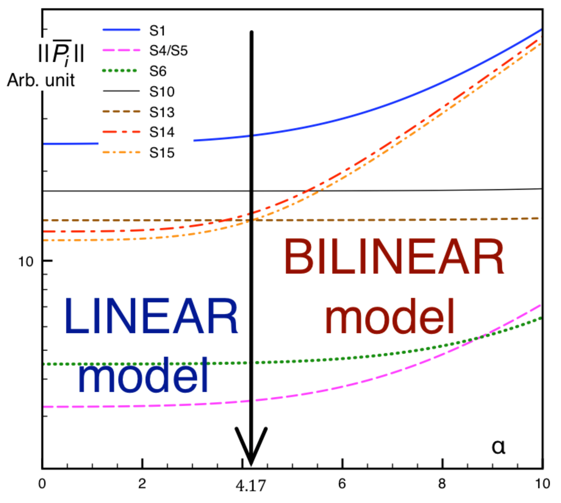
When the bilinear effects decrease, the proposed expansions allow a smooth transition to the linear case (see Property 3). This property can be useful in determining the range of applicability of a linear model and identifying generalized eigenmodes that are sensitive to bilinear effects and require “non-linear refinement” of their dynamics. It can be expected that in some large systems, there will be only a few such modes. Therefore, a non-linear examination of their dynamics will not take much time when real-time state estimation is required. The first test experiment with a bilinear model of an electric power system in [20] showed that the proposed spectral decompositions allow one to determine the range of applicability of linear model in general and to reveal particular generalized eigenmodes that sensitive to bilinear effects.

Although this study focuses on continuous bilinear systems, the results obtained can be extended to different classes of systems. First, they can be extended to discrete dynamical systems. In the linear case, this was partially performed in [18]. Meanwhile, the generalized Lyapunov equations that we consider for deterministic bilinear systems can be naturally associated with stochastic linear control systems (see [8]). Therefore, the results of spectral decomposition of Gramians can immediately be carried over to this class of systems. In this case, the results must be interpreted in terms of probabilities. Finally, the equations considered in this study can describe a special class of linear parameter-varying systems that can be reformulated as bilinear dynamical systems [9]. In this case, the interpretation of the spectral decompositions must include the effect of parameter variation.

It should be noted that the main object of research in this study is matrix Lyapunov equations, that is, matrix equations. An alternative approach is to apply the apparatus of linear matrix inequalities and semi-definite programming [25]. Therefore, another possible area of research is the combination of these approaches. In terms of applications, the authors plan to apply the developed methods to study the stability of electric power systems using linear and non-linear graph models. Another emerging area is the analysis of the stability of neural networks, including the use of Lyapunov functions [26,27]. The dissipativity principle in the synchronization of neural networks is very similar to the synchronization of generators in power systems. Therefore, the application of the developed methods to the problem of synchronization of neural networks is another possible direction for future research.

References

1. Häger, U.; Rehtanz, C.; Voropai, N.I. Monitoring, Control and Protection of Interconnected Power Systems; Springer: New York, NY, USA, 2014; 391p. [Google Scholar]
2. D’Alessandro, P.; Isidori, A.; Ruberti, A. Realization and structure theory of bilinear dynamic systems. SIAM J. Control. 1974, 12, 517–535. [Google Scholar] [CrossRef]
3. Pupkov, K.A.; Kapalin, V.I.; Yushchenko, A.S. Functional Series in the Theory of Nonlinear Systems; Nauka: Moscow, Russia, 1976; 448p. (In Russian) [Google Scholar]
4. Flagg, G.M.; Gugercin, S. Multipoint Volterra Series Interpolation and H2 Optimal Model Reduction of Bilinear Systems. SIAM J. Matrix Anal. Appl. 2015, 36, 549–579. [Google Scholar] [CrossRef] [Green Version]
5. Al-Baiyat, S.; Farag, A.S.; Bettayeb, M. Transient approximation of a bilinear two-area interconnected power system. Electr. Power Syst. Res. 1993, 26, 11–19. [Google Scholar] [CrossRef]
6. Zhang, L.; Lam, J. On the H2 model reduction of bilinear systems. Automatica 2002, 38, 205–216. [Google Scholar] [CrossRef]
7. Antoulas, A.C. Approximation of Large-Scale Dynamical Systems: Advances in Design and Control; SIAM: Philadephia, PA, USA, 2005; 479p. [Google Scholar]
8. Benner, P.; Breiten, T. Interpolation-based H2-model reduction of bilinear control systems. SIAM J. Matrix Anal. Appl. 2012, 33, 859–881. [Google Scholar] [CrossRef] [Green Version]
9. Benner, P.; Cao, X.; Schilders, W. A bilinear H2 model order reduction approach to bilinear parameter-varying systems. Adv. Comput. Math. 2019, 45, 2241–2271. [Google Scholar] [CrossRef] [Green Version]
10. Gibbard, M.J.; Pourbeik, P.; Vowles, D.J. Small-Signal Stability, Control and Dynamic Performance of Power Systems; University of Adelaide Press: Adelaide, Australia, 2015. [Google Scholar]
11. Jang, G.; Vittal, V.; Kliemann, W. Effect of nonlinear modal interaction on control performance: Use of normal forms technique in control design, Part 1: General theory and procedure. IEEE Trans. Power Syst. 1998, 13, 401–407. [Google Scholar] [CrossRef]
12. Pariz, N.; Shanechi, H.M.; Vaahedi, E. Explaining and validating stressed power systems behavior using modal series. IEEE Trans. Power Syst. 2003, 18, 778–785. [Google Scholar] [CrossRef]
13. Arroyo, J.; Betancourt, R.; Messina, A.R.; Barocio, E.D. Development of bilinear power system representations for small-signal stability analysis. Electr. Power Syst. Res. 2007, 77, 1239–1248. [Google Scholar] [CrossRef]
14. Ugwuanyi, N.S.; Kestelyn, X.; Thomas, O.; Marinescu, B.; Messina, A.R. New Fast Track to Nonlinear Modal Analysis of Power System Using Normal Form. IEEE Trans. Power Syst. 2020, 35, 3247–3257. [Google Scholar] [CrossRef] [Green Version]
15. Hamzi, B.; Abed, E.H. Local modal participation analysis of nonlinear systems using Poincaré linearization. Nonlinear Dyn. 2020, 99, 803–811. [Google Scholar] [CrossRef] [Green Version]
16. Benner, P.; Damm, T. Lyapunov equations, energy functionals, and model order reduction of bilinear and stochastic systems. SIAM J. Control. Optim. 2011, 49, 686–711. [Google Scholar] [CrossRef] [Green Version]
17. Yadykin, I.B.; Iskakov, A.B.; Akhmetzyanov, A.V. Stability analysis of large-scale dynamical systems by sub-Gramian approach. Int. J. Robust. Nonlin. Control 2014, 24, 1361–1379. [Google Scholar] [CrossRef]
18. Yadykin, I.B.; Iskakov, A.B. Spectral Decompositions for the Solutions of Sylvester, Lyapunov, and Krein Equations. Dokl. Math. 2017, 95, 103–107. [Google Scholar] [CrossRef]
19. Yadykin, I.B.; Iskakov, A.B. Spectral decompositions for the solutions of Lyapunov equations for bilinear dynamical systems. Dokl. Math. 2019, 100, 501–504. [Google Scholar] [CrossRef]
20. Iskakov, A.B.; Yadykin, I.B. Analysis of a bilinear model of an electric power system using spectral decompositions of Lyapunov functions. IFAC-PapersOnLine 2020, 53, 13514–13519. [Google Scholar] [CrossRef]
21. Garofalo, F.; Iannelli, L.; Vasca, F. Participation Factors and their Connections to Residues and Relative Gain Array. IFAC Proc. Vol. 2002, 35, 125–130. [Google Scholar] [CrossRef] [Green Version]
22. Bruni, C.; Dipillo, G.; Koch, G. On the mathematical models of bilinear systems. Ric. Di Autom. 1971, 2, 11–26. [Google Scholar]
23. Siu, T.; Schetzen, M. Convergence of Volterra series representation and BIBO stability of bilinear systems. Int. J. Syst. Sci. 1991, 22, 2679–2684. [Google Scholar] [CrossRef]
24. Yadykin, I.; Galyaev, A. On the methods for calculation of Gramians and their use in analysis of linear dynamic systems. Autom. Remote Control 2013, 74, 207–224. [Google Scholar] [CrossRef]
25. Khlebnikov, M.V. Quadratic Stabilization of Bilinear Control Systems. Autom. Remote Control 2016, 77, 980–991. [Google Scholar] [CrossRef]
26. Vadivel, R.; Hammachukiattikul, P.; Gunasekaran, N.; Saravanakumar, R.; Dutta, H. Strict dissipativity synchronization for delayed static neural networks: An event-triggered scheme. Chaos Solitons Fractals 2021, 150, 111212. [Google Scholar] [CrossRef]
27. Gunasekaran, N.; Thoiyab, N.M.; Zhu, Q.; Cao, J.; Muruganantham, P. New Global Asymptotic Robust Stability of Dynamical Delayed Neural Networks via Intervalized Interconnection Matrices. IEEE Trans. Cybern. 2021. [Google Scholar] [CrossRef] [PubMed]
Figure 1. The Frobenius norm of sub-Gramians P ˜ i for generalized eigenmodes as a function of the weighting coefficient α in the test experiment in [20].
Mathematics 09 03288 g001
Publisher’s Note: MDPI stays neutral with regard to jurisdictional claims in published maps and institutional affiliations.