Analytic Matrix Method for Frequency Response Techniques Applied to Nonlinear Dynamical Systems I: Small and Medium Amplitude Oscillations

Abstract

This is the first on a series of articles that deal with nonlinear dynamical systems under oscillatory input that may exhibit harmonic and non-harmonic frequencies and possibly complex behavior in the form of chaos. Frequency response techniques of nonlinear dynamical systems are usually analyzed with numerical methods because, most of the time, analytical solutions turn out to be difficult, if not impossible, since they are based on infinite series of trigonometric functions. The analytic matrix method reported here is a direct one that speeds up the solution processing compared to traditional series solution methods. In this method, we work with the invariant submanifold of the problem, and we propose a series solution that is equivalent to the harmonic balance series solution. However, the recursive relation obtained for the coefficients in our analytical method simplifies traditional approaches to obtain the solution with the harmonic balance series method. This method can be applied to nonlinear dynamic systems under oscillatory input to find the analog of a usual Bode plot where regions of small and medium amplitude oscillatory input are well described. We found that the identification of such regions requires both the amplitude as well as the frequency to be properly specified. In the second paper of the series, the method to solve problems in the field of large amplitudes will be addressed.

1. Introduction

Frequency response is a powerful technique to analyze the characteristics and properties of dynamical systems, describing the system response of a sinusoidal input with variable frequency. The system’s output magnitude and amplitude are both functions of the frequency; the output and input are then compared. The first frequency response technique (FRT) emerged in the 1930s during the development of the feedback amplifier stability [1]. Later on, it involved transfer functions to produce Nyquist and Bode plots, which are mainly used to study feedback amplifiers. Meanwhile, its antagonist, the time response approach, involved ordinary differential equations with their associated algebraic equations to solve problems related to automatic control systems needed in mechanical, naval and chemical engineering during WW1 [2]. However, as time went by, several FRTs were developed to solve problems in chemical engineering [3] and physical chemistry [4], among other areas.

In dynamical systems, when specific changes in the input (e.g., doubling the amplitude, two inputs summed, etc.) are reflected in the output spectrum (doubled amplitude, equivalent summed outputs, etc.), the systems are linear. For the specific case of time-invariant systems, the system response does not vary with time. Laplace transform is the method of solution of a linear system due to its simplicity by reducing ordinary differential equations to algebraic equations. For the frequency-response case, well-established stability criteria are important in the development of the frequency response methods in automatic control. To consult the classical FRT, the reader is referred to the collected works by MacFarlane [2].

Opposite to the behavior of a stable linear system under a periodic input (where an output of the same frequency is produced), a nonlinear system output oscillates with different frequencies with non-periodic harmonics that are not multiples of each other. The behavior of a nonlinear system that is not stable can be more complicated, i.e., one that is not at equilibrium nor periodic with near-periodic oscillations that evolve to chaos. Even though the system is deterministic in nature, some of these chaotic outputs exhibit randomness. The nonlinear system’s output may exhibit several modes of behavior and may have more than one limit cycle if the system is unforced. Conversely, a forced system with periodic input may produce complicated steady-state outputs that exhibit harmonic or subharmonic behavior; the kind of output produced usually depends on the amplitude and frequency of the input. It is worthwhile to mention that in some cases, when the amplitude or frequency of the input is smoothly changed, the nonlinear system may even exhibit a discontinuous jump in the output mode [2].

Among the methods proposed to solve the equations that arise in frequency response techniques, the Galerkin’s and Harmonic balance methods belong to the class of series solutions methods. Galerkin proposed a method to solve partial differential equations (PDE) that were too difficult to be solved analytically. This method turned out to be very useful to analyze complex PDE to find approximated solutions addressing the main concerns at the time: what residuals were to be used and how to be sure that the solutions actually converged. Galerkin was focused on the approximation to the solution by proposing a set of linearly independent test functions that are orthogonal to the residual. This method was tested first with a biharmonic equation and the results were published in 1915 [5]. Because of the flexibility of Galerkin’s approach, nowadays most of the known methods fall in this category, adopting the name of the contributor who developed a particular application [6]. The method of harmonic balance is another method belonging to the category of series solutions methods. In this case, the solution is proposed as the summation of exponential terms that capture the dependence with the amplitude, frequency and harmonics or sub-harmonics. Lately, this method has been used in several mechanical applications such as a bio-inspired work [7] or the study of nonlinear vibrations of a thin, polar-orthotropic circular plate [8]. The method of harmonic balance is a well-established method for the analysis of, for example, the power–frequency response to illustrate the effects of geometrical nonlinearity [9]. However, in the literature, the application of the method of harmonic balance and other methods to analyze the behavior of nonlinear systems subjected to FRT has been mostly using numeric approaches to particular study cases (see, for instance, [3,10,11,12,13]), and solving equations with the methods described previously can be challenging since the analytic approach may not be solvable and the numerical one does not provide an exact solution. To the best of our knowledge, there are no reported works on the general analytic solution for FRT.

In this paper, we present an analytic method for FRT with applications to nonlinear dynamical systems that is an improvement over the series solution methods available. This method provides a structured procedure to obtain information of nonlinear systems subjected to periodic inputs for the cases where the output is stable and others where the system is not at equilibrium. Hereby, we present some criteria to identify different modes of behavior such as the small amplitude oscillatory (SAOs) and the medium amplitude oscillatory (MAOs) that arise in several FRT applications. In the method reported here, we work with the invariant submanifold of the problem that is equivalent to the harmonic balance series solution. The recursive relation obtained for the coefficients in our analytical method simplifies traditional approaches to obtain the solution with the harmonic balance series method.

2. Preliminary

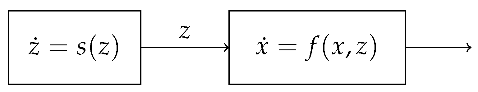
Consider a pair of cascade interconnected systems of the form (see Figure 1).

$$\begin{array}{ccc}\hfill \dot{x}& =& f\left(x,z\right)\hfill \end{array}$$

(1)

$$\begin{array}{ccc}\hfill \dot{z}& =& s\left(z\right)\hfill \end{array}$$

(2)

where $x\in {\mathbb{R}}^n$, $z\in {\mathbb{R}}^m$, $f\left(0,0\right)=0$, $s\left(0\right)=0$, and $f\left(x,z\right)$, $s\left(z\right)$ are locally Lipschitz in ${\mathbb{R}}^n\times {\mathbb{R}}^m$. $\dot{x}$ and $\dot{z}$ represent the time derivative of x and z, respectively. The state variables z of system (2) can be seen as an input vector of system (1); therefore, system (2) is called the driving (or master) system of the tested (or slave) system (1), which is considered to be input-state stable. According to the input-state stability theory of dynamical systems [14], the tested system input-state is stable if for $z=0$ the unforced system (1)

$$\dot{x}\left(t\right)=f\left(x\left(t\right),0\right)$$

(3)

is asymptotically stable, i.e., that $∥x\left(t\right)∥\to 0$ as $t\to \infty$, and for a input $z\left(t\right)$ with finite supreme norm ${∥z\left(·\right)∥}_{\infty }={sup}_{t\ge 0}∥z\left(t\right)∥$, it holds that

$$∥x\left(t\right)∥\le \beta \left(∥x\left(0\right)∥,t\right)+\gamma \left({∥z\left(·\right)∥}_{\infty }\right)$$

(4)

where $\gamma \left(·\right)$ is a class $\mathcal{K}$ function (a continuous function $\gamma :\left[0,a\right)\to \left[0,\infty \right)$ is said to belong to the class $\mathcal{K}$ if it is strictly increasing and $\gamma \left(0\right)=0$ [15].) and $\beta$ is a class $\mathcal{KL}$ function (a continuous function $\beta :\left[0,a\right)\times \left[0,\infty \right)\to \left[0,\infty \right)$ is said to belong to the class $\mathcal{KL}$ if, for each fixed s, the mapping $\beta \left(r,s\right)$ belongs to class $\mathcal{K}$ with respect to r and, for each fixed r, the mapping $\beta \left(r,s\right)$ is decreasing with respect to s and $\beta \left(r,s\right)\to 0$ as $r\to \infty$[15]).Then, given the properties of the class $\mathcal{KL}$ function $\beta$, it holds that ${lim}_{t\to \infty }∥x\left(t\right)∥=\gamma \left({∥z\left(·\right)∥}_{\infty }\right)$, i.e., that the behavior of $x\left(t\right)$ synchronizes with the behavior of $z\left(t\right)$. This implies that the state variable, $x\left(t\right)$, reaches an invariant submanifold, $x\left(t\right)=\xi \left(z\left(t\right)\right)$, that depends exclusively on the behavior of $z\left(t\right)$, i.e., any trajectory $x\left(t\right)$ of the system (6) is the image through the mapping $\pi \left(·\right)$ of a trajectory of the driving system. Note that the mapping $\xi :z\to x$ is in general an immersion, i.e., the rank is equal to the dimension of z that satisfies the partial differential equation

$$\frac{\partial \xi \left(z\right)}{\partial z}s\left(z\right)=f\left(\xi \left(z\right),z\right).$$

(5)

Figure 1. Cascade interconnected subsystems.

In particular, if the driving system (2) is Poisson stable, i.e., its dynamical behavior has persistent oscillations with maximum amplitude A, then ${lim}_{t\to \infty }∥x\left(t\right)∥=\gamma \left(\left|A\right|\right)$, and the tested system (1) might also tend to a Poisson stable behavior in the invariant submanifold, with maximum amplitude bounded by $\gamma \left(\left|A\right|\right)$. This result can be applied to the analysis of FRT, as shown in the following section.

3. Frequency Response Analysis

Consider the input-state stable dynamical system

$$\dot{x}\left(t\right)=f\left(x\left(t\right),z\left(t\right)\right)$$

(6)

where $x\in X\subset {\mathbb{R}}^n$ is the state vector, while $z\in {\mathbb{R}}^2$ is the input vector and $f:X\times {\mathbb{R}}^2\to {\mathbb{R}}^n$ is a continuous function. In particular, in traditional FRT, z has a linear oscillatory behavior with the following dynamics

$$\begin{array}{ccc}\hfill {\dot{z}}_1& =& \omega z_2\hfill \end{array}$$

(7)

$$\begin{array}{ccc}\hfill {\dot{z}}_2& =& -\omega z_1\hfill \end{array}$$

(8)

where $\omega$ is the frequency of oscillation. The behavior of $z_1$ and $z_2$ depends on the initial conditions and has the general form: $z_1\left(t\right)=Asin\left(\omega t+\varphi \right)$ and $z_2\left(t\right)=Acos\left(\omega t+\varphi \right)$, where A and $\varphi$ are the amplitude and phase of oscillation.

Notice that the oscillator (7) and (8) is Poisson stable and is a particular case of system (2), while system (6) is similar to system (1) assuming input-state stability; therefore, $x\left(t\right)$ will reach an invariant submanifold, $x\left(t\right)=\xi \left(z\left(t\right)\right)$, that satisfies a partial differential equation analogous to Equation (5), i.e.,

$$\dot{\xi }\left(z\right)=f\left(\xi \left(z\right),z\right)$$

(9)

where for the oscillator (7) and (8), in particular, the time derivative of $\dot{\xi }$ is

$$\dot{\xi }=\omega \left(\frac{\partial \xi }{\partial z_1}{z}_2-\frac{\partial \xi }{\partial z_2}{z}_1\right).$$

For instance, consider a simple pendulum swinging under gravity and frictional viscous damping, whose dynamical behavior can be represented by the following equation

$$ml\frac{d^2\theta }{d{t}^2}=-mgsin\left(\theta \right)-\mu \frac{d\theta }{dt}+\frac{T}{l}$$

(10)

where $\theta$ is the angular position, m is the mass concentrated in the tip, l is the length of the pendulum, g is the gravity acceleration, $\mu$ is the friction coefficient and T is the applied torque. For simplicity purposes, let us define the following dimensionless variables $\tau =\sqrt{g/l}t$, $\eta =\mu /\left(m\sqrt{gl}\right)$, $x_1=\theta$, $x_2=d\theta /d\tau$ and $u=T/\left(mgl\right)$, then the dynamical model becomes

$$\begin{array}{ccc}\hfill {\dot{x}}_1& =& x_2\hfill \end{array}$$

(11)

$$\begin{array}{ccc}\hfill {\dot{x}}_2& =& -sin\left(x_1\right)-\eta x_2+u\hfill \end{array}$$

(12)

Notice that when $u=0$, the steady-state is given by $x_2=0$ and $sin\left(x_1\right)=0$; therefore, $x_1=\pm n\pi$, for $n=0,1,2,3,\dots$, and given the stability properties, the only stable equilibrium points are $x_1=\pm 2n\pi$, for $n=0,1,2,3,\dots$. Then, if the pendulum is submitted to an oscillatory torque: $u\left(t\right)=z_1\left(t\right)$, where $z_1$ is the first element of the state vector of the oscillator (7) and (8), for small frequencies, after a transient behavior that depends on the initial conditions, the pendulum will approach to an invariant submanifold $x\left(t\right)=\xi \left(z\left(t\right)\right)$, which satisfies the following pair of nonlinear coupled partial differential equations:

$$\begin{array}{ccc}\hfill \omega \left(\frac{\partial {\xi }_1}{\partial z_1}{z}_2-\frac{\partial {\xi }_1}{\partial z_2}{z}_1\right)& =& {\xi }_2,\hfill \end{array}$$

(13)

$$\begin{array}{ccc}\hfill \omega \left(\frac{\partial {\xi }_2}{\partial z_1}{z}_2-\frac{\partial {\xi }_2}{\partial z_2}{z}_1\right)& =& -sin\left({\xi }_1\right)-\eta {\xi }_2+z_1.\hfill \end{array}$$

(14)

In the following section, a method is proposed to solve this class of equations.

4. Analytical Matrix Method

One procedure to find periodic solutions of nonlinear systems is the method of harmonic balance [15]. This method assumes that the solution can be represented by a linear combination of sinusoids (a Fourier series) of the form:

$$y\left(t\right)=\sum _{k=-\infty }^{\infty }{a}_{k}exp\left(ik\omega t\right)$$

(15)

where $\omega$ is the main frequency with harmonics of the form $k\omega$, for $k\in \mathbb{Z}$. The problem reduces to find the frequency and Fourier coefficients $a_k$. In the present work, an analogous procedure is proposed, namely, it is assumed that each element of the invariant submanifold, $\pi \left(z\right)$, that satisfies Equation (9), has the following form

$${\xi }_k\left(z\right)=\sum _{i=0}^{\infty }\sum _{j=0}^{\infty }{c}_{k,i,j}{z}_1^i{z}_2^j,k=1,2,\dots ,n$$

(16)

where $c_{k,i,j}$ are undetermined coefficients. Then, the problem reduces to find the correct value of these coefficients, that can be found using the quadrature method, where the proposed solution (16) is substituted in Equation (9) to reduce the problem to find coefficients $c_{k,i,j}$. This solution can be rewritten in matrix form as

$${\xi }_k=Z_1^T{C}_k{Z}_2$$

(17)

where

$$Z_i=\left(\begin{array}{c}1\\ z_i\\ z_i^2\\ ⋮\end{array}\right),\mathrm{for}i=1,2,$$

(18)

and

$$C_k=\left(\begin{array}{cccc}{c}_{k,0,0}& c_{k,0,1}& c_{k,0,2}& \cdots \\ c_{k,1,0}& c_{k,1,1}& c_{k,1,2}& \cdots \\ c_{k,2,0}& c_{k,2,1}& c_{k,2,2}& \cdots \\ ⋮& ⋮& ⋮& \ddots \end{array}\right).$$

(19)

Now it is possible to state the problem to be solved in the present work.

Problem 1.

Given the tested system (6) submitted to a oscillatory regimen by the driving system (7) and (8), after the transient period, system (6) reaches a invariant submanifold, $x\left(t\right)=\xi \left(z\left(t\right)\right)$, described by the invariance partial differential equation

$$\omega \left(\frac{\partial \xi \left(z\right)}{\partial z_1}{z}_2-\frac{\partial \xi \left(z\right)}{\partial z_2}{z}_1\right)=f\left(\xi \left(z\right),z\right).$$

(20)

Then, the problem to be solved is to find an analytical series solution with the form (17) that satisfies Equation (20).

Notice that instead of using a harmonics series, such as Equation (15), in the proposed series solution (16), the driving variables, $z_1$ and $z_2$, are elevated to integer powers and the use of the matrix form (17) allows simplifying the analysis and solution in a more systematic way. The following two definitions are instrumental for developing the proposed solution method.

Definition 1.

Given two square matrices ${\Phi }_a$ and ${\Phi }_b$ with the same dimension $N\times N$ (N could tend to infinity), the product operator is defined as

$${⟨{\Phi }_a,{\Phi }_b⟩}_N=\sum _{k=0}^{N-1}\left[\left(\begin{array}{ccccc}{\Phi }_a{E}_k& P^T{\Phi }_a{E}_k& {\left(P^2\right)}^T{\Phi }_a{E}_k& \cdots & {\left(P^{N-1}\right)}^T{\Phi }_a{E}_k\end{array}\right){\Phi }_b{P}^k\right]$$

(21)

where the elements of matrix P are

$${\left[P\right]}_{i,j}=\left\{\begin{array}{cc}1\hfill & \mathrm{if}j=i+1\hfill \\ 0\hfill & \mathrm{otherwise}\hfill \end{array}\right.,$$

(22)

while E is a vector of dimension $N\times 1$, whose elements are

$${\left[E_k\right]}_{i,1}=\left\{\begin{array}{cc}1\hfill & \mathrm{if}i=k+1\hfill \\ 0\hfill & otherwise\hfill \end{array}\right..$$

(23)

Definition 2.

Given the square matrix ${\Phi }_a$ of dimension $N\times N$, the differential operator is defined as

$$d{\Phi }_a=D^T{\Phi }_{a}P-P^T{\Phi }_{a}D$$

(24)

where the elements of matrix D are

$${\left[D\right]}_{i,j}=\left\{\begin{array}{cc}j\hfill & \mathrm{if}i=j+1\hfill \\ 0\hfill & otherwise\hfill \end{array}\right.,$$

(25)

while the elements of matrix P are defined in Equation (22).

To substitute the proposed solution (16) in Equation (9), it is necessary to compute the time derivative of $\pi$; given that $\pi$ is the sum of coefficients of the form $z_1^i{z}_2^j$, with $i,j\in \mathbb{N}$, its time derivative is

$$\frac{d}{dt}\left(z_1^i{z}_2^j\right)=i{z}_1^{i-1}{z}_2^j{\dot{z}}_1+j{z}_1^i{z}_2^{j-1}{\dot{z}}_2$$

(26)

and considering the dynamics of z, given in Equations (7) and (8), it holds that

$$\frac{d}{dt}\left(z_1^i{z}_2^j\right)=\omega \left(i{z}_1^{i-1}{z}_2^{j+1}-j{z}_1^{i+1}{z}_2^{j-1}\right).$$

(27)

Notice that the sum of exponents of $z_1^i{z}_2^j$ is $i+j$ and, given the linear dynamics of z, the sum of exponents of $\frac{d}{dt}\left(z_1^i{z}_2^j\right)$ is preserved and equal to $i+j$. Following this structure, the time derivative of the infinite series (16), or its matrix form (17), is presented in the following Proposition.

Proposition 1.

Consider the square matrix ${\Phi }_a$ of infinite dimension with constant coefficients, associated to a function of $z_1$ and $z_2$ defined as

$${\varphi }_a\left(z_1\left(t\right),z_2\left(t\right)\right)=Z_1^T\left(t\right){\Phi }_a{Z}_2\left(t\right)$$

(28)

where vectors $Z_1\left(t\right)$ and $Z_2\left(t\right)$ are defined in Equation (18). The time derivative of ${\varphi }_a$ is

$$\frac{d}{dt}\left[{\varphi }_a\left(z_1\left(t\right),z_2\left(t\right)\right)\right]=\omega Z_1^T\left(t\right)\left(d{\Phi }_a\right)Z_2\left(t\right)$$

(29)

where $d{\Phi }_a$ is the operator described in Definition 2.

Proof. 

Notice that the derivative of vector $Z_i$ with respect to $z_i$ is

$$d{Z}_i=\left(\begin{array}{c}0\\ 1\\ 2z_i\\ 3z_i^2\\ ⋮\end{array}\right)=D{Z}_i,i=1,2$$

(30)

where

$$D=\left(\begin{array}{cccc}0& 0& 0& \cdots \\ 1& 0& 0& \cdots \\ 0& 2& 0& \cdots \\ 0& 0& 3& \ddots \\ ⋮& ⋮& \ddots & \ddots \end{array}\right)$$

(31)

is defined in Equation (25). Therefore, the partial derivatives of ${\varphi }_a$ with respect to $z_1$ and $z_2$ are

$$\begin{array}{ccc}\hfill \frac{\partial {\varphi }_a}{\partial z_1}=\frac{\partial {\varphi }_a}{\partial Z_1}d{Z}_1& =& Z_2^T{\Phi }_a^{T}D{Z}_1\hfill \end{array}$$

(32)

$$\begin{array}{ccc}\hfill \frac{\partial {\varphi }_a}{\partial z_2}=\frac{\partial {\varphi }_a}{\partial Z_2}d{Z}_2& =& Z_1^T{\Phi }_{a}D{Z}_2\hfill \end{array}$$

(33)

On the other hand, notice that

$$Z_i{z}_i^n=P^n{Z}_i,\mathrm{for}i=1,2$$

(34)

where

$$P=\left(\begin{array}{ccccc}0& 1& 0& 0& \cdots \\ 0& 0& 1& 0& \cdots \\ 0& 0& 0& 1& \ddots \\ ⋮& ⋮& \ddots & \ddots & \ddots \end{array}\right),$$

(35)

is defined in Equation (22); therefore, the time derivative of ${\varphi }_a$ is

$$\frac{d{\varphi }_a}{dt}=\omega Z_1^T\left(D^T{\Phi }_{a}P-P^T{\Phi }_{a}D\right)Z_2.$$

(36)

Finally, with Definition 2, it holds that ${\dot{\varphi }}_a=\omega Z_1^T\left(d{\Phi }_a\right)Z_2$, concluding the proof. □

Equation (6) contains nonlinear term; therefore, it might have products of finite or infinite series of $z_1$ and $z_2$. For instance, the product $z_1^a{z}_2^b$ where $a,b\in \mathbb{Z}$ can be expressed in matrix form as

$$z_1^a{z}_2^b=Z_1^T{B}_{a,b}{Z}_2$$

(37)

where

$${\left[B_{a,b}\right]}_{i,j}=\left\{\begin{array}{cc}1\hfill & \mathrm{if}i=a+1\wedge j=b+1\hfill \\ 0\hfill & \mathrm{otherwise}\hfill \end{array}\right.,$$

(38)

while the procedure to compute the product of two series is presented in the following proposition.

Proposition 2.

Consider the square matrices ${\Phi }_a$ and ${\Phi }_b$ with infinite dimension, associated to functions ${\varphi }_a$ and ${\varphi }_b$ of $z_1$ and $z_2$ defined as

$$\begin{array}{ccc}\hfill {\varphi }_a\left(z_1\left(t\right),z_2\left(t\right)\right)& =& Z_1^T\left(t\right){\Phi }_a{Z}_2\left(t\right),\hfill \end{array}$$

(39)

$$\begin{array}{ccc}\hfill {\varphi }_b\left(z_1\left(t\right),z_2\left(t\right)\right)& =& Z_1^T\left(t\right){\Phi }_b{Z}_2\left(t\right);\hfill \end{array}$$

(40)

the product of these functions is

$${\varphi }_a\left(z_1\left(t\right),z_2\left(t\right)\right){\varphi }_b\left(z_1\left(t\right),z_2\left(t\right)\right)=\left(Z_1^T\left(t\right){\Phi }_a{Z}_2\left(t\right)\right)\left(Z_1^T\left(t\right){\Phi }_b{Z}_2\left(t\right)\right),$$

(41)

which is equivalent to

$${\varphi }_a\left(z_1\left(t\right),z_2\left(t\right)\right){\varphi }_b\left(z_1\left(t\right),z_2\left(t\right)\right)=Z_1^T\left(t\right){⟨{\Phi }_a,{\Phi }_b⟩}_{\infty }{Z}_2\left(t\right)$$

(42)

where the operator ${⟨{\Phi }_a,{\Phi }_b⟩}_N$ is described in Definition 1.

Proof. 

${\varphi }_a\left(z_1,z_2\right)$ is a scalar function; therefore, Equation (41) is equivalent to

$$\begin{array}{ccc}\hfill {\varphi }_a\left(z_1,z_2\right){\varphi }_b\left(z_1,z_2\right)& =& \left(\begin{array}{cccc}{\varphi }_a& {\varphi }_a{z}_1& {\varphi }_a{z}_1^2& \cdots \end{array}\right){\Phi }_b{Z}_2\hfill \\ & =& \left(\begin{array}{cccc}{Z}_1^T{\Phi }_a{Z}_2& z_1{Z}_1^T{\Phi }_a{Z}_2& z_1^2{Z}_1^T{\Phi }_a{Z}_2& \cdots \end{array}\right){\Phi }_b{Z}_2\hfill \end{array}$$

and considering Equation (34), the previous equation is equivalent to

$${\varphi }_a\left(z_1,z_2\right){\varphi }_b\left(z_1,z_2\right)=Z_1^T\left(\begin{array}{cccc}{\Phi }_a{Z}_2& P^T{\Phi }_a{Z}_2& {\left(P^2\right)}^T{\Phi }_a{Z}_2& \cdots \end{array}\right){\Phi }_b{Z}_2.$$

Notice that, using matrices $E_k$, defined in Equation (23), $Z_2$ can be expressed as

$$Z_2=\sum _{k=0}^{\infty }{E}_k{z}_2^k$$

therefore

$${\varphi }_a\left(z_1,z_2\right){\varphi }_b\left(z_1,z_2\right)=Z_1^T\sum _{k=0}^{\infty }\left(\begin{array}{cccc}\left({\Phi }_a{E}_k\right)& \left(P^T{\Phi }_a{E}_k\right)& \left({\left(P^2\right)}^T{\Phi }_a{E}_k\right)& \cdots \end{array}\right){\Phi }_b{z}_2^k{Z}_2$$

and finally, using Equation (34) again, it holds that

$$\begin{array}{ccc}\hfill {\varphi }_a\left(z_1,z_2\right){\varphi }_b\left(z_1,z_2\right)& =& Z_1^T\left(\begin{array}{cccc}{\Phi }_a{E}_0& P^T{\Phi }_a{E}_0& {\left(P^2\right)}^T{\Phi }_a{E}_0& \cdots \end{array}\right){\Phi }_b{Z}_2\hfill \\ & & +Z_1^T\left(\begin{array}{cccc}{\Phi }_a{E}_1& P^T{\Phi }_a{E}_1& {\left(P^2\right)}^T{\Phi }_a{E}_1& \cdots \end{array}\right){\Phi }_{b}P{Z}_2\hfill \\ & & +Z_1^T\left(\begin{array}{cccc}{\Phi }_a{E}_2& P^T{\Phi }_a{E}_2& {\left(P^2\right)}^T{\Phi }_a{E}_2& \cdots \end{array}\right){\Phi }_b{P}^2{Z}_2+\cdots \hfill \end{array}$$

(43)

From here it is possible to define matrix

$${⟨{\Phi }_a,{\Phi }_b⟩}_N=\sum _{k=0}^{N-1}\left[\left(\begin{array}{ccccc}{\Phi }_a{E}_k& P^T{\Phi }_a{E}_k& {\left(P^2\right)}^T{\Phi }_a{E}_k& \cdots & {\left(P^{N-1}\right)}^T{\Phi }_a{E}_k\end{array}\right){\Phi }_b{P}^k\right],$$

as described in Equation (21), in order to rewrite Equation (43) as

$${\varphi }_a\left(z_1,z_2\right){\varphi }_b\left(z_1,z_2\right)=Z_1^T{⟨{\Phi }_a,{\Phi }_b⟩}_{\infty }{Z}_2,$$

concluding the proof. □

Finally, the following theorem presents the conditions to find the oscillatory invariant submanifolds.

Theorem 1.

Given the input-state stable differential Equation (6), with $x\in X\in {\mathbb{R}}^n$ and $z\in {\mathbb{R}}^2$, and the oscillatory dynamics defined in Equations (7) and (8), assume that $x\left(t\right)$ reaches an invariant submanifold that satisfies Equation (20).

Then, if function $f\left(x\left(t\right),z\left(t\right)\right)$ can be expressed as series of integer powers of the elements of x and z, the solution of each element of vector π can be proposed to be an infinite series of integer powers of $z_1$ and $z_2$, i.e.,

$${\xi }_k\left(t\right)=\sum _{i=0}^{\infty }\sum _{j=0}^{\infty }{c}_{k,i,j}{z}_1^i\left(t\right)z_2^j\left(t\right),k=1,2,\dots ,n,$$

(44)

that in matrix form is

$${\xi }_k\left(t\right)=Z_1^T\left(t\right)C_k{Z}_2\left(t\right),k=1,2,\dots ,n$$

(45)

where matrices $C_k$ are

$$C_k=\left(\begin{array}{cccc}{c}_{k,0,0}& c_{k,0,1}& c_{k,0,2}& \cdots \\ c_{k,1,0}& c_{k,1,1}& c_{k,1,2}& \cdots \\ c_{k,2,0}& c_{k,2,1}& c_{k,2,2}& \cdots \\ ⋮& ⋮& ⋮& \ddots \end{array}\right).$$

(46)

Proof. 

The system of differential equations defined in Equation (20) is

$$\omega \left(\frac{\partial {\xi }_k\left(z\right)}{\partial z_1}{z}_2-\frac{\partial {\xi }_k\left(z\right)}{\partial z_2}{z}_1\right)=f_k\left({\xi }_1\left(z\right),\dots {\xi }_n\left(z\right),z_1,z_2\right),k=1,2,\dots ,n.$$

Assume that the elements of the invariant submanifold $\pi \left(t\right)$ can be described as in Equation (45), then, according to Proposition 1, their time derivatives are

$$\frac{d{\xi }_k\left(t\right)}{dt}=\omega Z_1^T\left(t\right)\left(d{C}_k\right)Z_2\left(t\right),k=1,2,\dots ,n,$$

where $d{C}_k=D^T{C}_{k}P-P^T{C}_{k}D$. Using this time derivative, the elements of Equation (20) become

$$0=\omega Z_1^T\left(t\right)\left(d{C}_k\right)Z_2\left(t\right)-f_k\left(Z_1^T{C}_1{Z}_2,\dots ,Z_1^T\left(t\right)C_n{Z}_2\left(t\right),z_1,z_2\right),$$

for $k=1,2,\dots ,n$. If functions $f_k\left(x,z\right)$ can be expressed as series of integer powers of the elements of x and z, then using identities given in Equations (37) and (42) in Proposition 2, it can be shown that functions $f_k\left(x,z\right)$ are equivalent to

$$f_k\left(Z_1^T{C}_1{Z}_2,\dots ,Z_1^T\left(t\right)C_n{Z}_2\left(t\right),z_1,z_2\right)=Z_1^T{F}_k\left(C_1,\dots ,C_n\right)Z_2$$

and the differential equations can be transformed to the form

$$0=Z_1^T\left[\omega d{C}_k-F_k\left(C_1,\dots ,C_n\right)\right]Z_2,k=1,2,\dots ,n$$

(47)

where $F_k\left(C_1,\dots ,C_n\right)$ is a matrix that depends on the values of coefficient matrices $C_1,\dots ,C_n$, defined in Equation (46). Independently of the values of vectors $Z_1$ and $Z_2$, Equation (47) holds if

$$\omega d{C}_k-F_k\left(C_1,\dots ,C_n\right)=0,k=1,2,\dots ,n,$$

(48)

then the problem reduces to finding coefficients $c_{k,i,j}$, $k=1,2,\dots ,n$, $i,j\in \mathbb{N}$, by solving Equations (48) to obtain the solution given in Equation (45). □

By looking at invariant Equation (47), we can infer that the matrix Equation (48) depend on the applied frequency $\omega$; therefore, the values of coefficient matrices $C_1,\dots ,C_n$ also depend on this frequency. Once these coefficients (46) have been determined, it is possible to analyze the system’s behavior in the frequency domain. Since $z_1=Asin\left(\omega t\right)$ and $z_2=Acos\left(\omega t\right)$, then

$${\xi }_k\left(t\right)=\sum _{n=0}^{\infty }{A}^n\sum _{i=0}^n{c}_{k,n-i,i}{sin}^{n-i}\left(\omega t\right){cos}^i\left(\omega t\right),k=1,2,\dots ,n$$

(49)

Notice that the trigonometric properties: $2sin\left(\alpha \right)sin\left(\beta \right)=cos\left(\alpha -\beta \right)-cos\left(\alpha +\beta \right)$, $2cos\left(\alpha \right)cos\left(\beta \right)=cos\left(\alpha -\beta \right)+cos\left(\alpha +\beta \right)$, and $2sin\left(\alpha \right)cos\left(\beta \right)=sin\left(\alpha -\beta \right)+sin\left(\alpha +\beta \right)$, allow verifying that solution (49) is equivalent to the proposed solution of the method of harmonic balance (15). On the other hand, the series (49) is convergent if the amplitude is small enough in comparison with the values of coefficients $c_{k,i,j}$ that are fixed by the applied frequency. Therefore, we can define the following oscillations modes:

Definition 3.

Consider the norm of the coefficients of series (49) with the same order: $∥c_{k,n}∥={\left({\sum }_{i=1}^n{c}_{k,n-i,i}^2\right)}^{1/2}$. The possible oscillations modes are the following:

 SAOs 

If $∥c_{k,n}∥>A∥c_{k,n+1}∥$ for $n=1,2,3,\dots$ and $A\ll ∥c_{k,1}∥/∥c_{k,2}∥$, then system (9) is in Small Amplitude Oscillations mode (SAOs); therefore, the terms with order two or higher are negligible, and solution (49) reduces to ${\xi }_k\left(t\right)\approx c_{k,0,0}+A\left[c_{k,1,0}sin\left(\omega t\right)\right.\left.+c_{k,0,1}cos\left(\omega t\right)\right]$.

 MAOs 

If $∥c_{k,n}∥>A∥c_{k,n+1}∥$ for $n=1,2,3,\dots$, then system (9) is in Medium Amplitude Oscillations mode (MAOs) and additional terms of higher-order in solution (49) must be included to describe its oscillatory response correctly.

 LAOs 

Finally, if the series is not convergent, i.e., $∥c_{k,n}∥\ngtr A∥c_{k,n+1}∥$ as n increases, then system (9) is in Large Amplitude Oscillations mode (LAOs) and solution (49) is not longer suitable to describe the behavior of system (9).

Since the current contribution is focused on the analysis of SAOs and MAOs modes, the LAOs analysis will be left to a future contribution.

5. Study Cases

5.1. Series Solutions for a Simple Globally Asymptotically Stable Model

To illustrate the proposed method, consider the following dynamical system:

$$\dot{x}=-x^3+u$$

(50)

where $x\in \mathbb{R}$ is the state variable and $u\in \mathbb{R}$ is the input variable. Notice that when $u=0$, the steady-state is given by $x=0$, and using the Lyapunov function $V=x^2$, it is straightforward to verify that this equilibrium is globally asymptotically stable, because $\dot{V}=-2x^4=-2V^2<0$ for $V\ne 0$. Then, if system (50) is submitted to an oscillatory input: $u\left(t\right)=z_1\left(t\right)$, where $z_1$ is the first element of the state vector of the oscillator (7)–(8), after a transient behavior that depends on the initial conditions, the system will approach an invariant submanifold, $x\left(t\right)=\xi \left(z\left(t\right)\right)$, that satisfies the following nonlinear partial differential equation:

$$\omega \left(\frac{\partial \xi }{\partial z_1}{z}_2-\frac{\partial \xi }{\partial z_2}{z}_1\right)=-{\xi }^3+z_1$$

(51)

To find the analytical solution, it is considered that $\pi$ can be expressed as a series of the form of Equation (17), i.e.,

$$\xi =Z_1^{T}C{Z}_2.$$

(52)

with unknown coefficients matrix C. The time derivative of the invariant submanifold is

$$\dot{\xi }=\omega \left(\frac{\partial \xi }{\partial z_1}{z}_2-\frac{\partial \xi }{\partial z_2}{z}_1\right)=\omega Z_1^{T}dC{Z}_2,$$

where $dC=D^{T}CP-P^{T}CD$, while the first term of the right-hand side of Equation (51) is ${\xi }^3=Z_1^T{Q}_3{Z}_2$, where $Q_3={⟨C_1,{⟨C_1,C_1⟩}_{\infty }⟩}_{\infty }$, and the second term of the right-hand side of Equation (51) is $z_1=Z_1^T{A}_{1,0}{Z}_2$; therefore, Equation (51) becomes

$$0=Z_1^T\left(\omega dC+Q_3-B_{1,0}\right)Z_2$$

which is satisfied for any oscillatory behavior iff

$$0=\omega dC+Q_3-B_{1,0}.$$

(53)

Equation (53) allows to compute the matrix of coefficients C, and following the procedure described in Appendix A, the solution of Equation (51) is

$$\begin{array}{ccc}\hfill \xi \left(t\right)& =& -\frac{1}{\omega }{z}_2\left(t\right)+\frac{2z_1^3\left(t\right)+3z_1\left(t\right)z_2^2\left(t\right)}{3{\omega }^4}+\frac{13z_2^5\left(t\right)+10z_1^2\left(t\right)z_2^3\left(t\right)}{15{\omega }^7}\hfill \\ & & -\frac{52z_1^7\left(t\right)+232z_1^5\left(t\right)z_2^2\left(t\right)+219z_1^3\left(t\right)z_2^4\left(t\right)+195z_1\left(t\right)z_2^6\left(t\right)}{75{\omega }^{10}}+\cdots \hfill \end{array}$$

(54)

Notice that each term in Equation (54) has the form $z_1^i{z}_2^j$, satisfying the condition that the total order $n=i+j$ is an odd number. System (50) is in SAOs mode when the terms with order two or bigger are negligible, i.e., $\xi \left(t\right)\approx -\frac{1}{\omega }{z}_2\left(t\right)$, while this system is in MAOs mode when additional terms of higher order must be included to correctly describe its oscillatory response. Given the coefficients of the analytical solution (54), SAOs occurs when $A^2\ll {\omega }^3$.

Figure 2 shows the predictions with a numeric method solution and the analytical solution (54) truncated up to first-order, $\xi \left(t\right)=-\frac{1}{\omega }{z}_2\left(t\right)$, third-order, $\xi \left(t\right)=-\frac{1}{\omega }{z}_2\left(t\right)+\frac{2z_1^3\left(t\right)+3z_1\left(t\right)z_2^2\left(t\right)}{3{\omega }^4}$, and seventh-order (see Equation (54)).

Figure 2. Comparison of system behavior using numeric and analytic solutions (54) for $\omega =0.5$, $A=0.2$ and $\varphi =0$ ($T=2\pi /\omega$). (a) u vs. $t/T$, (b) x vs. $t/T$, and (c) phase plane $\left(x,u\right)$.

5.2. Series Solutions for a Simple Pendulum

Now, consider the pendulum model presented in Section 3. The oscillatory invariant submanifold for this pendulum satisfies Equations (13) and (14). Now the solution is proposed to have the form of Equation (17), i.e.,

$${\xi }_1=Z_1^T{C}_1{Z}_2\mathrm{and}{\xi }_2=Z_1^T{C}_2{Z}_2,$$

(55)

where $Z_i$ for $i=1,2$ is defined in Equation (18). Given that $sin\left({\pi }_1\right)={\sum }_{j=0}^{\infty }\frac{{\left(-1\right)}^j{\pi }_1^{2j+1}}{\left(2j+1\right)!}$, using Proposition 2, the sine function in Equation (14) is

$$sin\left({\pi }_1\right)=Z_1^T{\Omega }_{\sin }{Z}_2$$

(56)

where

$${\Omega }_{\sin }=\sum _{j=0}^{\infty }\frac{{\left(-1\right)}^j}{\left(2j+1\right)!}{W}_j$$

(57)

with $W_0=C_1$,

$$W_j=⟨W_{j-1},W_C⟩,j=1,2,3,\dots$$

and $W_C=⟨C_1,C_1⟩$. According to Proposition 1, ${\dot{\xi }}_i=\omega Z_1^T\left(d{C}_i\right)Z_2$, while the term $z_1$ is equivalent to $Z_1^T{A}_{1,0}{Z}_2$; therefore, Equations (13) and (14) can be expressed as

$$\begin{array}{ccc}\hfill \omega Z_1^T\left(d{C}_1\right)Z_2& =& Z_1^T{C}_2{Z}_2,\hfill \\ \hfill \omega Z_1^T\left(d{C}_2\right)Z_2& =& -Z_1^T{\Omega }_{\sin }{Z}_2-\eta Z_1^T{C}_2{Z}_2+Z_1^T{B}_{1,0}{Z}_2.\hfill \end{array}$$

or

$$\begin{array}{ccc}\hfill Z_1^T\left(\omega d{C}_1-C_2\right)Z_2& =& 0,\hfill \\ \hfill Z_1^T\left(\omega d{C}_1+{\Omega }_{\sin }+\eta C_2-B_{1,0}\right)Z_2& =& 0.\hfill \end{array}$$

Independently of the values of vectors $Z_1$ and $Z_2$, Equation (13) holds if

$$\omega d{C}_1-C_2=0$$

(58)

while Equation (14) holds if

$$\omega d{C}_2+{\Omega }_{\sin }+\eta C_2-B_{1,0}=0$$

(59)

where $d{C}_i$ for $i=1,2$ are the differential operators described in Proposition 1. Equations (58) and (59) are a particular case of Equation (48). The coefficients $C_1$ and $C_2$ are obtained by solving the matrix Equations (58) and (59), as shown in Appendix B. Thus, the behavior of the pendulum angular position and angular velocity are

$$\begin{array}{ccc}\hfill {\xi }_1\left(\tau \right)& =& \pm n\pi -\frac{\left({\omega }^2-{\left(-1\right)}^n\right)z_1\left(\tau \right)+\eta \omega z_2\left(\tau \right)}{{\left({\omega }^2-{\left(-1\right)}^n\right)}^2+{\left(\eta \omega \right)}^2}\hfill \end{array}$$

$$\begin{array}{ccc}& & +\frac{q_{3,0}{z}_1^3\left(\tau \right)+q_{2,1}{z}_1^2\left(\tau \right)z_2\left(\tau \right)+q_{1,2}{z}_1\left(\tau \right)z_2^2\left(\tau \right)+q_{0,3}{z}_2^3\left(\tau \right)}{{\left({\left(\eta \omega \right)}^2+{\left[{\omega }^2-{\left(-1\right)}^n\right]}^2\right)}^3\left({\left(3\eta \omega \right)}^2+{\left[{\left(3\omega \right)}^2-{\left(-1\right)}^n\right]}^2\right)}+\cdots \hfill \\ \hfill {\xi }_2\left(\tau \right)& =& \omega \frac{\eta \omega z_1\left(\tau \right)-\left({\omega }^2-{\left(-1\right)}^n\right)z_2\left(\tau \right)}{{\left({\omega }^2-{\left(-1\right)}^n\right)}^2+{\left(\eta \omega \right)}^2}\hfill \\ & & -\frac{\omega \left[q_{2,1}{z}_1^3\left(\tau \right)-q_{1,2}{z}_2^3\left(\tau \right)\right]}{{\left({\left(\eta \omega \right)}^2+{\left[{\omega }^2-{\left(-1\right)}^n\right]}^2\right)}^3\left({\left(3\eta \omega \right)}^2+{\left[{\left(3\omega \right)}^2-{\left(-1\right)}^n\right]}^2\right)}\hfill \end{array}$$

(60)

$$\begin{array}{ccc}& & -\frac{\omega \left[\left(2q_{1,2}-3q_{3,0}\right)z_1\left(\tau \right)+\left(3q_{0,3}-2q_{2,1}\right)z_2\left(\tau \right)\right]z_1\left(\tau \right)z_2\left(\tau \right)}{{\left({\left(\eta \omega \right)}^2+{\left[{\omega }^2-{\left(-1\right)}^n\right]}^2\right)}^3\left({\left(3\eta \omega \right)}^2+{\left[{\left(3\omega \right)}^2-{\left(-1\right)}^n\right]}^2\right)}+\cdots \hfill \end{array}$$

(61)

where

$$\begin{array}{ccc}\hfill q_{3,0}& =& {\eta }^2{\omega }^2\left(\frac{1}{2}{\left(-1\right)}^n+2{\omega }^2-{\eta }^2{\omega }^2{\left(-1\right)}^n-\frac{21}{2}{\omega }^4{\left(-1\right)}^n\right)\hfill \\ & & +\frac{21}{2}{\omega }^8{\left(-1\right)}^n-\frac{71}{3}{\omega }^6+16{\omega }^4{\left(-1\right)}^n-3{\omega }^2+\frac{{\left(-1\right)}^n}{6}\hfill \\ \hfill q_{2,1}& =& -\eta \omega \left({\eta }^2{\omega }^2-24{\omega }^6{\left(-1\right)}^n+33{\omega }^4-10{\omega }^2{\left(-1\right)}^n+1\right)\hfill \\ \hfill q_{1,2}& =& -{\omega }^2\left(\frac{3}{2}{\eta }^4{\omega }^2{\left(-1\right)}^n+\frac{9}{2}{\eta }^2{\omega }^4{\left(-1\right)}^n+6{\eta }^2{\omega }^2\right.\hfill \\ & & \left.-\frac{5}{2}{\eta }^2{\left(-1\right)}^n-9{\omega }^6{\left(-1\right)}^n+19{\omega }^4-11{\omega }^2{\left(-1\right)}^n+1\right)\hfill \\ \hfill q_{0,3}& =& \eta {\omega }^3\left(3{\eta }^2{\omega }^2{\left(-1\right)}^n-\frac{8}{3}{\eta }^2+19{\omega }^4{\left(-1\right)}^n-22{\omega }^2+3{\left(-1\right)}^n\right)\hfill \end{array}$$

while the remaining coefficients can be easily obtained with Equation (A6). According to Theorem 1, the invariant submanifold will be only reached if the system is input-state stable, and given that the pendulum has two classes of equilibrium points: (1) $x_1=\pm \left(2n+1\right)\pi$ (up) and 2) $x_1=\pm 2n\pi$ (down) for $n=0,1,2,\dots$. Therefore, the family of “up” fixed points are unstable, while the “down” fixed points are stable; therefore, the correct solutions of Equations (60) and (61) are those where n is equal to zero or an even number. This analytical solution is compared with a numerical solution for two different cases in Figure 3 and Figure 4. Figure 3a and Figure 4a show the time evolution of the angular position, Figure 3b and Figure 4b show the time evolution of the angular velocity, and Figure 3c and Figure 4c show the phase plane with respect to the oscillatory driving signal.

Figure 3. Comparison of the pendulum behavior predictions using the numeric and analytic solution (60) and (61) ($N_{max}=3$) for $\eta =0.1428$, $n=0$, $\omega =1.2$, $A=0.1$ and $\varphi =\pi /3$ ($T=2\pi /\omega$). (a) $x_1$ vs. $\tau /T$, (b) $x_2$ vs. $\tau /T$, and (c) phase plane $\left(x_1,x_2,u\right)$.

Figure 4. Comparison of the pendulum behavior predictions using the numeric and analytic solution (60) and (61) ($N_{max}=11$) for $\eta =0.1428$, $n=0$, $\omega =0.05$, $A=0.9$ and $\varphi =0$ ($T=2\pi /\omega$). (a) $x_1$ vs. $\tau /T$, (b) $x_2$ vs. $\tau /T$, and (c) phase plane $\left(x_1,x_2,u\right)$.

6. Discussion

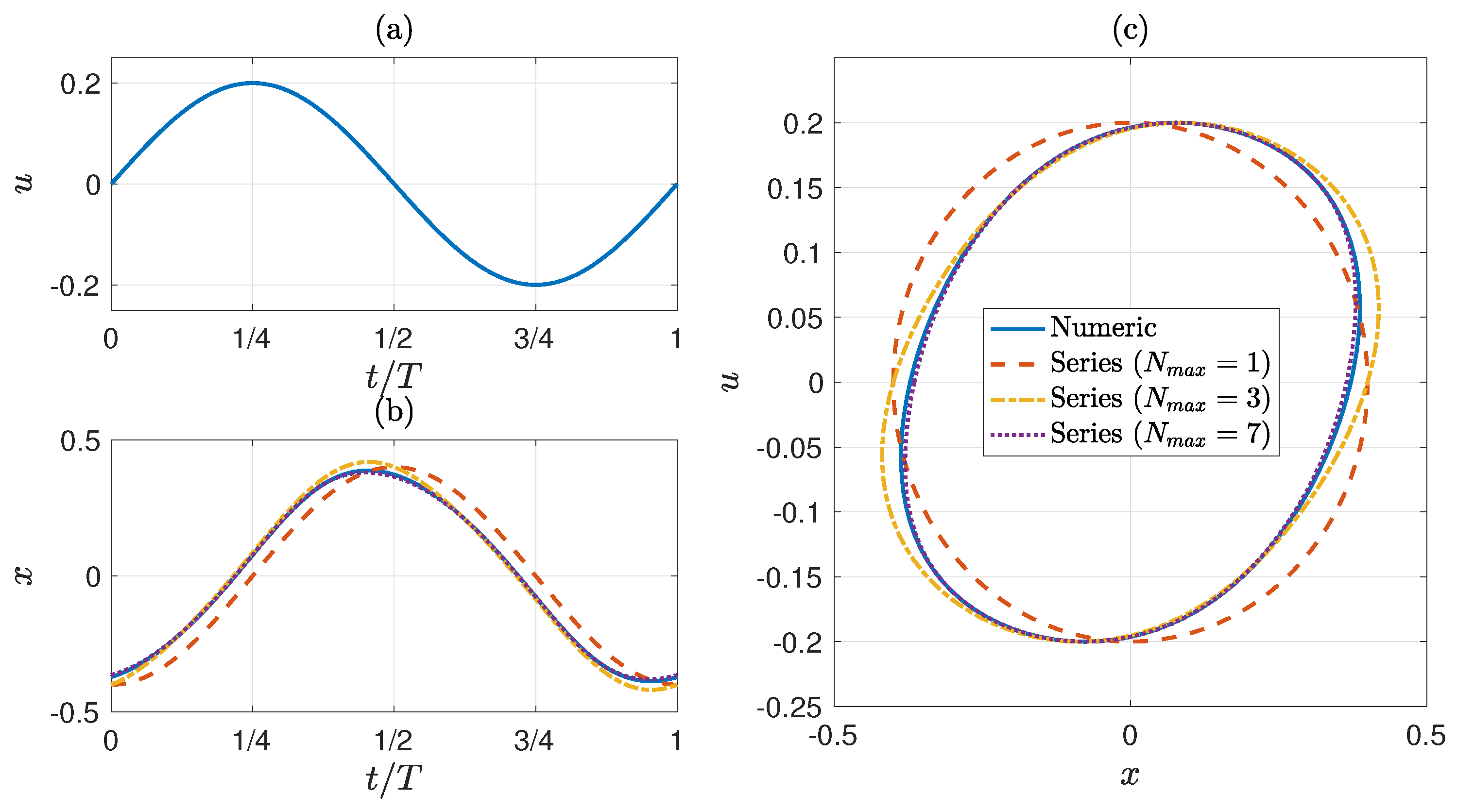
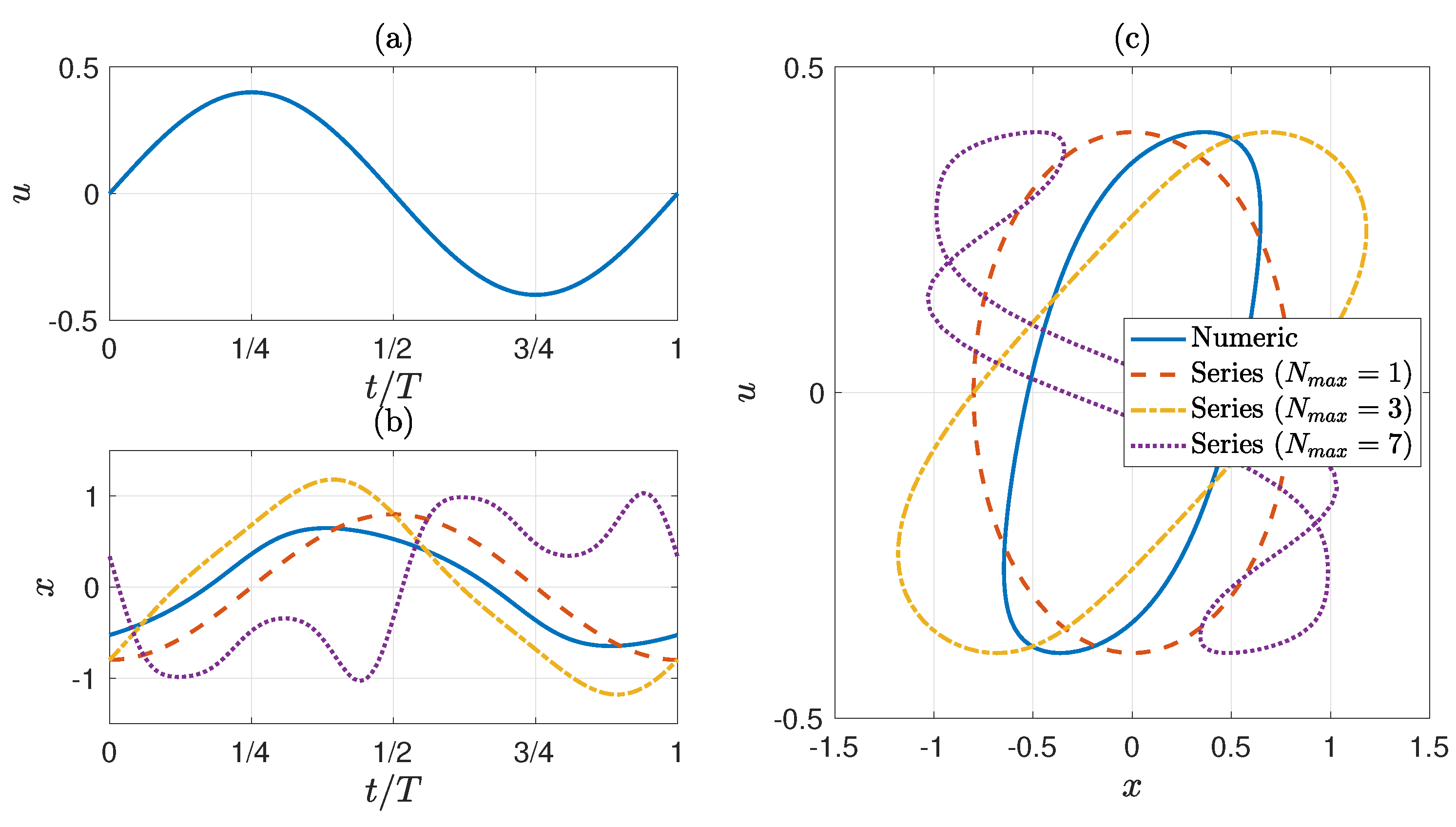
For the study case of the series solutions for a simple globally asymptotically stable model, Figure 2 shows that the analytical solutions truncated up to the first-order and third-order are unable to reproduce the behavior, while the analytical solution truncated up to seventh-order satisfactorily describes the system behavior. Notice that, by looking in Equation (54) at the coefficients of the series and considering that $z_1=Asin\left(\omega t+\varphi \right)$ and $z_2=Acos\left(\omega t+\varphi \right)$, it holds that the first-order term ($n=1$) is proportional to $A/\omega$, while the third, fifth and seventh-order terms ($n=3,4,5$) are proportional to $A^3/{\omega }^4$, $A^5/{\omega }^7$, and $A^7/{\omega }^{10}$, respectively. Following this sequence, the terms of order $n=2k-1$, for $k=1,2,3,\dots$, are proportional to $A^{2k-1}/{\omega }^{3k-2}$. Thus, the convergence of series (54) is correlated to the convergence of coefficient ${\left(A^2/{\omega }^3\right)}^k\left({\omega }^2/A\right)$ with respect to k, then, without considering the constant coefficients in series (54), an approximated limit to guarantee the convergence of series is that the relation frequency–amplitude must satisfy ${\omega }^3>A^2$; if this relation is satisfied then we can say that the system is in SAOs mode when $A^2/{\omega }^3\ll 1$ or MAOs mode when ${\omega }^3>A^2$, respectively. In Figure 2, $\omega =0.5$ and $A=0.2$ were selected, which satisfies the aforementioned relation, while Figure 5 shows the predictions for the same frequency but with an amplitude $A=0.4$, which violates the relation ${\omega }^3>A^2$, and therefore, the analytical solution Equation (54) is no longer suitable for describing the dynamical behavior because, in this context, the system is in LAOs mode. To make the analysis in LAOs mode, it would be necessary to reconsider the assumption $C_{2,0}=0$ made to solve Equation (A1), which actually has an infinite number of solutions of the form $C_{0,2}=C_{2,0}$; therefore, if $C_{2,0}\ne 0$, it would appear a term of the form $C_{2,0}{A}^2\left[{sin}^2\left(\omega t+\varphi \right)+{cos}^2\left(\omega t+\varphi \right)\right]$ that is equivalent to $C_{2,0}{A}^2$. Therefore, a new constant term would appear, modifying the equation $\left(i,j\right)=\left(0,0\right)$ of system (53), i.e., instead of $0=C_{0,0}^3$, it would be $0=C_{0,0}^3+C_{2,0}{A}^2$, and now $C_{0,0}$ could be different to zero and a function of the amplitude. The complete analysis of LAOs mode will be left to a future contribution.

Figure 5. Comparison of system behavior predictions using numeric and analytic solution (54) for $\omega =0.5$, $A=0.4$ and $\varphi =0$ ($T=2\pi /\omega$). (a) u vs. $\tau /T$, (b) x vs. $\tau /T$, and (c) phase plane $\left(x,u\right)$.

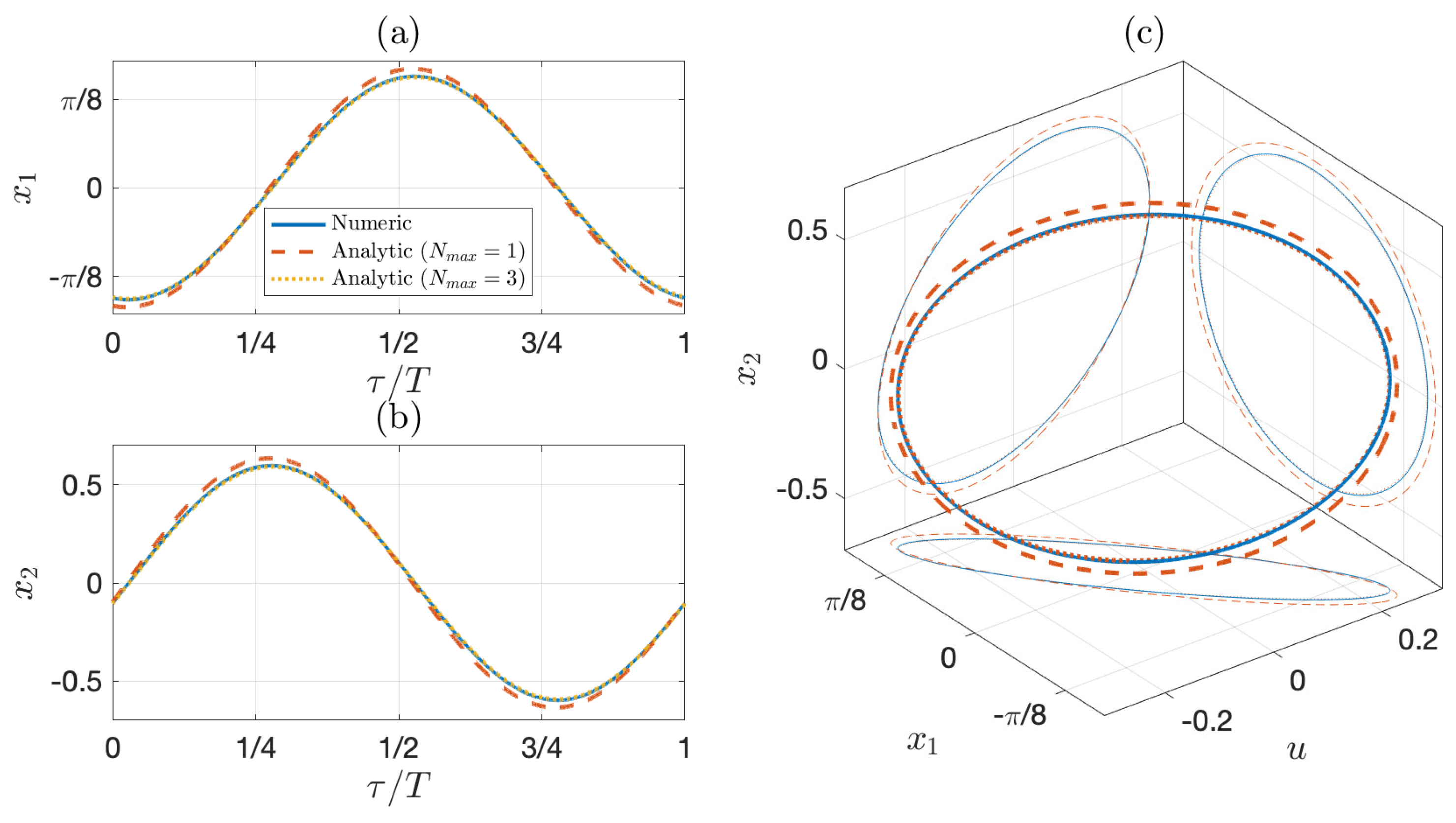
Notice that for the well-known problem of a simple pendulum that oscillates under sinusoidal potentials, the resonance characteristics are difficult to find by solving the problem analytically; hence, the numerical approach is the method of choice [16]. However, we were able to find the analytical solution for the study case of the series solutions for a simple pendulum. We found that when the system behaves almost as in the SAOs regime (Figure 3), there may be deviations from the linear behavior and additional third-order terms must be included to accurately reproduce the system’s behavior.

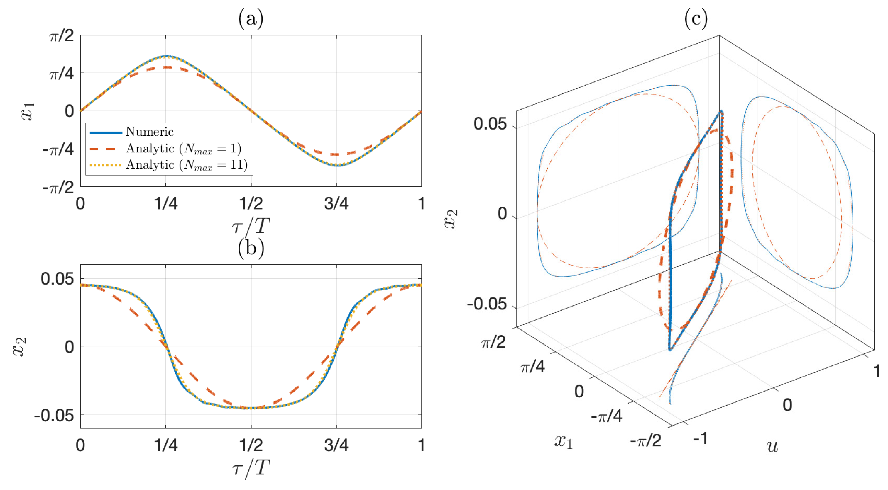
Figure 4 depicts the system in a MAOs regime with more pronounced nonlinear characteristics, where coefficients up to eleventh order must be included to correctly reproduce the system’s behavior.

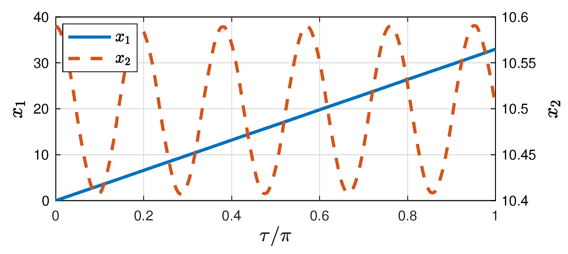
Figure 6 shows that for $\omega =0$, $z_1$ becomes constant and the steady-state solution of Equations (11) and (12) is given by the equations $x_2=0$ and $0=z_1-sin\left(x_1\right)$; therefore, $x_1=\pm 2n\pi +arcsin\left(z_1\right)$, where n may be equal to $n=0,1,2,\dots$. However this solution is only feasible if $z_1\le 1$, because given the domain of sine function, if $z_1>1$, this class of steady-state is not longer feasible and the pendulum reaches a permanent regime where $\left|x_1\right|$ keeps growing, while $x_2$ oscillates around a constant value, i.e., the pendulum rotates persistently. Consequently, solution (60) is not longer valid to describe this behavior, because according to Theorem 1, the system described in Equation (12) is not longer input-state stable. An example of this behavior is shown Figure 6. In this case, the system is not longer in a SAOs or MAOs regimen.

Figure 6. Dynamical behavior of the pendulum under permanent growth of $x_1$ for a constant value of $z_1>1$ ($\eta =0.1428$, $\omega =0$, $A=1.5$ and $\varphi =0$).

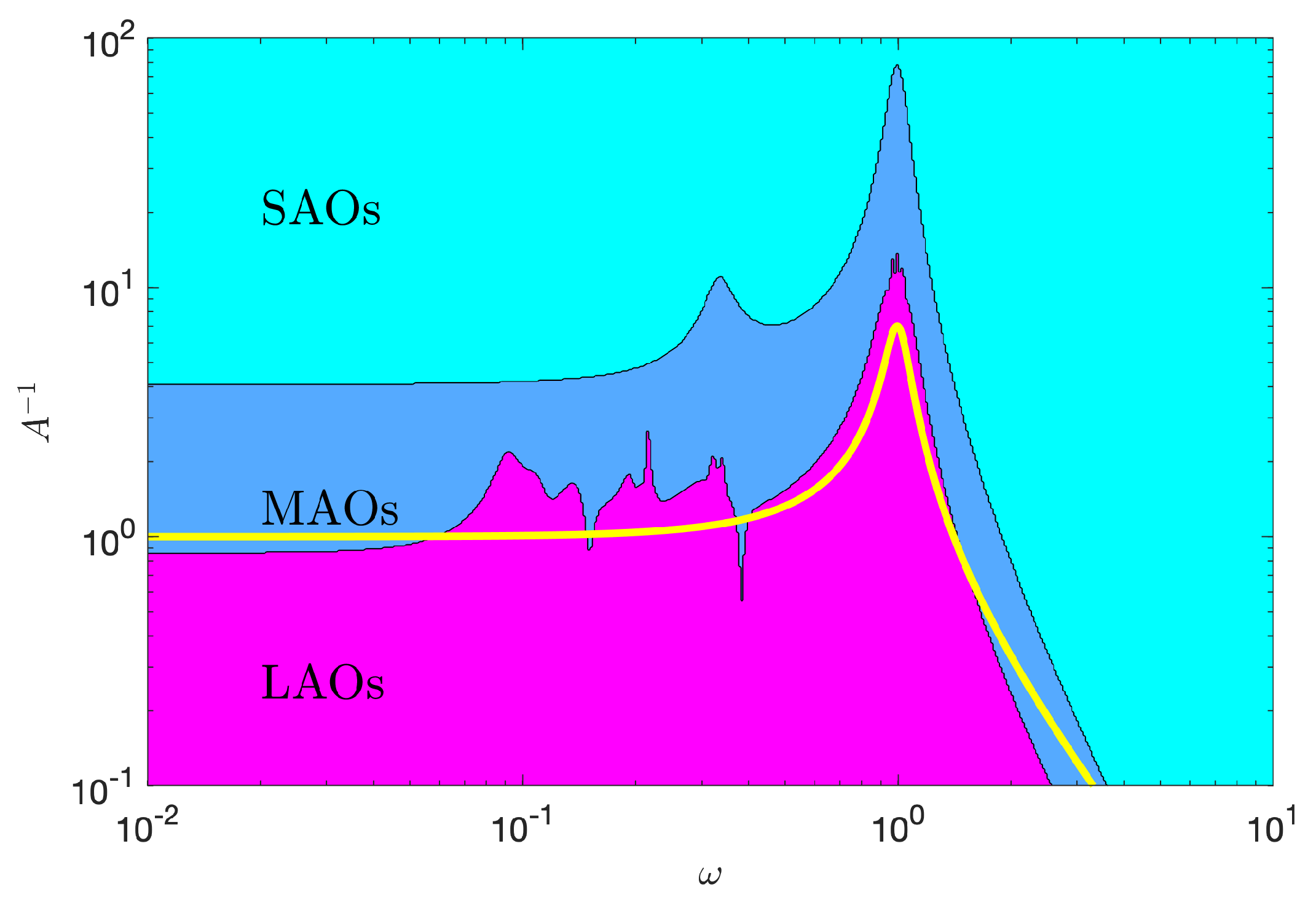
To analyze the approximated regions in which SAOs, MAOs, or LAOs hold for the angular position of the pendulum, it is possible to use Definition 3 in the coefficients ${\widehat{C}}_{1,k}$, given in Equation (A6). Figure 7 sketches these regions as a function of the applied frequency and amplitude. In particular, the boundary between SAOs and MAOs regions was selected to have a maximum 1% variation with respect to the linear behavior, i.e., where $A=0.01∥c_{1,1}∥/∥c_{1,2}∥$ and $∥c_{1,n}∥>A∥c_{1,n+1}∥$ for $n=1,2,3,\dots$, while the boundary between SAOs and MAOs regions approximates the points at which solution (60) is not longer suitable to describe the oscillatory behavior because $∥c_{1,n}∥\ngtr A∥c_{1,n+1}∥$ for some $n=1,2,3,\dots$. As can be seen, for low frequencies and for amplitudes approximately bigger than 1, the pendulum is in LAOs mode, while for high frequencies the SAOs mode predominates regardless of the amplitude. Particularly for frequencies around 1, the boundaries between the three regions appears at smaller amplitudes, because this frequency is the natural frequency of the pendulum (given the numerical value of the damping parameter, the eigenvalues of the Jacobian around equilibrium are approximately $0.0714\pm 0.9974i$), and the driving force is producing larger resonances. Another resonance region is approximately at frequencies between 0.1 and 0.4, associated with the damping constant $\eta$. Finally, notice that the diagram in Figure 7 has some similarities with the typical amplitude ratio Bode plot for a second-order damped system, which for comparison purposes was superimposed on the diagram (yellow line), suggesting that this class of diagram may be a valuable tool for frequency response techniques of nonlinear systems.

Figure 7. Approximated regions of the pendulum’s oscillation modes as a function of frequency and amplitude ($\eta =0.1428$).

7. Conclusions

The analytic method for FRT with applications to nonlinear dynamical systems presented here is an improvement over the series solution methods available because it offers the possibility of obtaining the analytical solution. This method provides a structured procedure by working with the invariant submanifold of the problem that is equivalent to the harmonic balance series solution. The recursive relation obtained for the coefficients in our analytical method simplifies traditional approaches to obtain the solution with the harmonic balance series method. This proved to be useful to obtain information of nonlinear systems subjected to periodic inputs for the cases where the output is stable and others where the system is not at equilibrium. Furthermore, this method is useful to identify the modes of behavior SAOs and MAOs that arise in several FRT applications; the criteria to explore LAOs will be presented in a second paper of the series.

References

1. Nyquist, H. Regeneration Theory. Bell Syst. Tech. J. 1932, 11, 126–147. [Google Scholar] [CrossRef]
2. MacFarlane, A.G. Chapter Part II. The Classical Frequency-Response Techniques. In Frequency-Response Methods in Control Systems; IEEE Press: New York, NY, USA, 1979; pp. 17–139. [Google Scholar]
3. Petkovska, M.; Nikolić, D.; Seidel-Morgenstern, A. Nonlinear Frequency Response Method for Evaluating Forced Periodic Operations of Chemical Reactors. Isr. J. Chem. 2018, 58, 663–681. [Google Scholar] [CrossRef]
4. Wang, Y. Identification of mass transfer resistances in microporous materials using frequency response methods. Adsorption 2021, 27, 369–395. [Google Scholar] [CrossRef]
5. Galerkin, B. Series solution of some problems of elastic equilibrium of rods and plates. Vestn. Inzh. Tekh. 1915, 19, 897–908. [Google Scholar]
6. Repin, S. One Hundred Years of the Galerkin Method. Comp. Meth. Appl. Math. 2017, 17, 351–357. [Google Scholar] [CrossRef]
7. Song, Y.; Zhang, C.; Li, Z.; Li, Y.; Lian, J.; Shi, Q.; Yan, B. Study on dynamic characteristics of bio-inspired vibration isolation platform. J. Vib. Control. 2021. [Google Scholar] [CrossRef]
8. Rai, A.K.; Gupta, S.S. Nonlinear vibrations of a polar-orthotropic thin circular plate subjected to circularly moving point load. Compos. Struct. 2021, 256, 112953. [Google Scholar] [CrossRef]
9. Lu, Z.Q.; Ding, H.; Chen, L.Q. Resonance response interaction without internal resonance in vibratory energy harvesting. Mech. Syst. Signal Process. 2019, 121, 767–776. [Google Scholar] [CrossRef]
10. Frank Pai, P. Time–frequency analysis for parametric and non-parametric identification of nonlinear dynamical systems. Mech. Syst. Signal Process. 2013, 36, 332–353. [Google Scholar] [CrossRef]
11. Živković, L.A.; Milić, V.; Vidaković-Koch, T.; Petkovska, M. Rapid Multi-Objective Optimization of Periodically Operated Processes Based on the Computer-Aided Nonlinear Frequency Response Method. Processes 2020, 8, 1357. [Google Scholar] [CrossRef]
12. Zhu, Y.; Lang, Z. The effects of linear and nonlinear characteristic parameters on the output frequency responses of nonlinear systems: The associated output frequency response function. Automatica 2018, 93, 422–427. [Google Scholar] [CrossRef]
13. Zhu, Y.P.; Lang, Z.; Mao, H.L.; Laalej, H. Nonlinear output frequency response functions: A new evaluation approach and applications to railway and manufacturing systems’ condition monitoring. Mech. Syst. Signal Process. 2022, 163, 108179. [Google Scholar] [CrossRef]
14. Isidori, A. Nonlinear Control Systems II; Springer: London, UK, 1999. [Google Scholar]
15. Khalil, H. Nonlinear Systems, 3rd ed.; Prentice-Hall: Hoboken, NJ, USA, 2002. [Google Scholar]
16. Kharkongor, D.; Mahato, M.C. Resonance oscillation of a damped driven simple pendulum. Eur. J. Phys. 2018, 39, 065002. [Google Scholar] [CrossRef] [Green Version]