
Deep Learning Models for Predicting Monthly TAIEX to Support Making Decisions in Index Futures Trading


Abstract
:1. Introduction
- We have proposed an approach to apply time series modeling based on deep learning for predicting MAT.
- We performed extensive experiments to evaluate three different deep learning architectures on the task of supporting decision-making in trading MTX contracts.
- We proposed and compared the effectiveness of two simple stop-loss strategies that can help avoid losses in trading index futures using predictive models.
2. Literature Review
3. Background
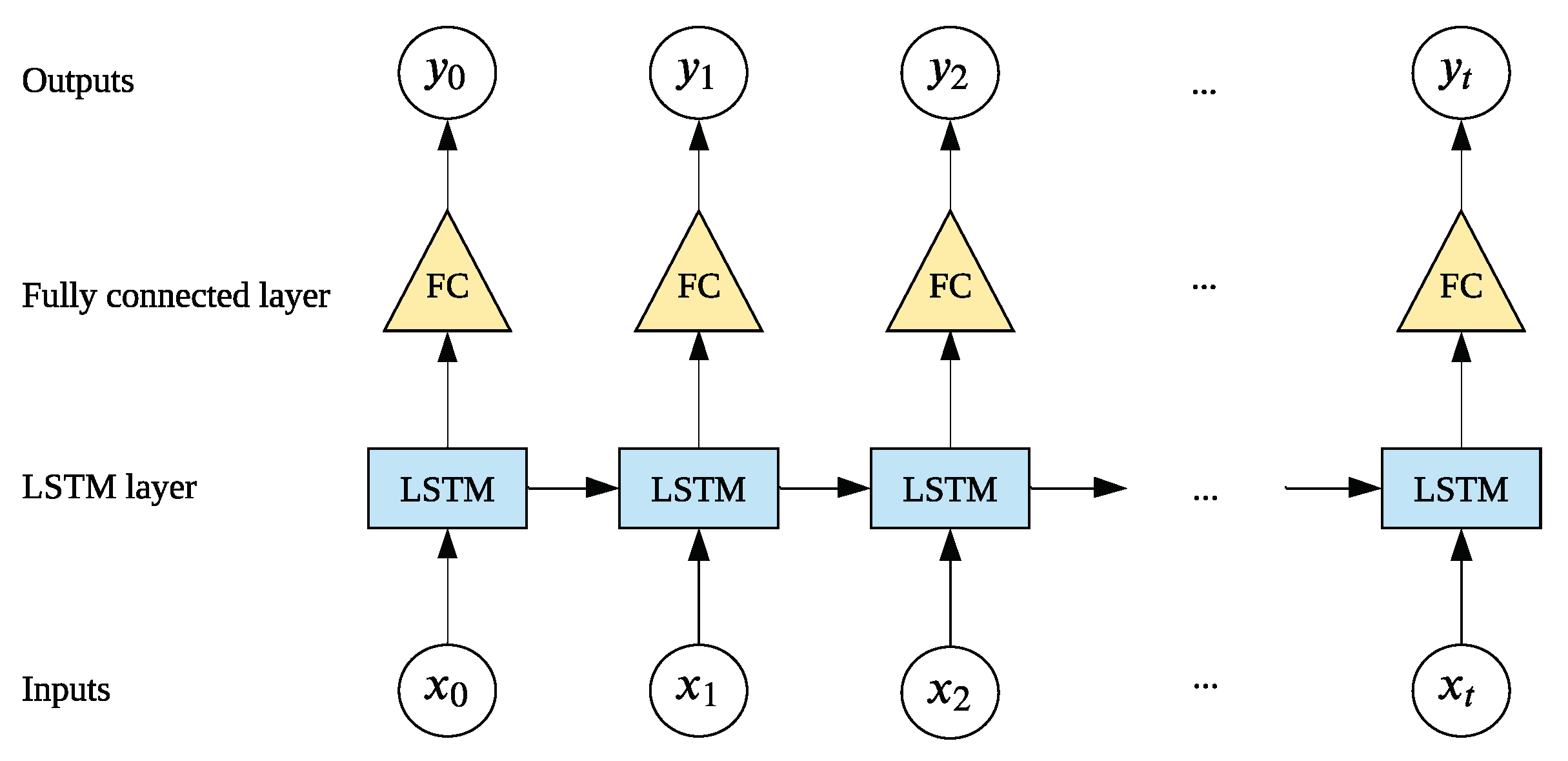
3.1. LSTM
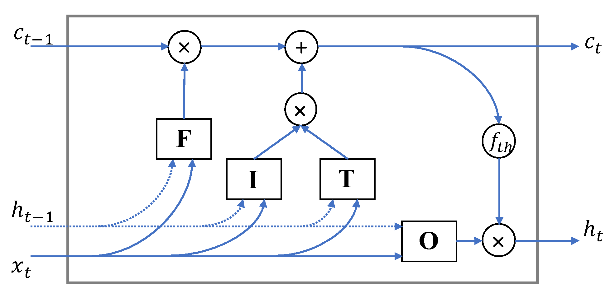
- The forget gate F defines which things should be forgotten in cell state .
- The input gate I cooperates with gate T to update the cell state with new input and the previous hidden state .
- The output gate O specifies what information from the new cell state is used to generate the new hidden state . The new hidden state is also used as the output of the LSTM block.
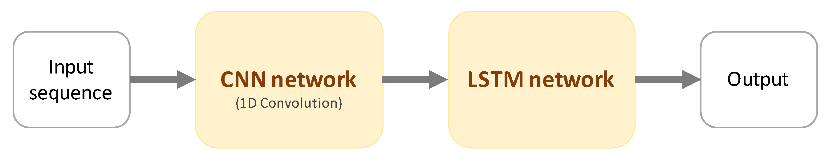
3.2. CNN-LSTM
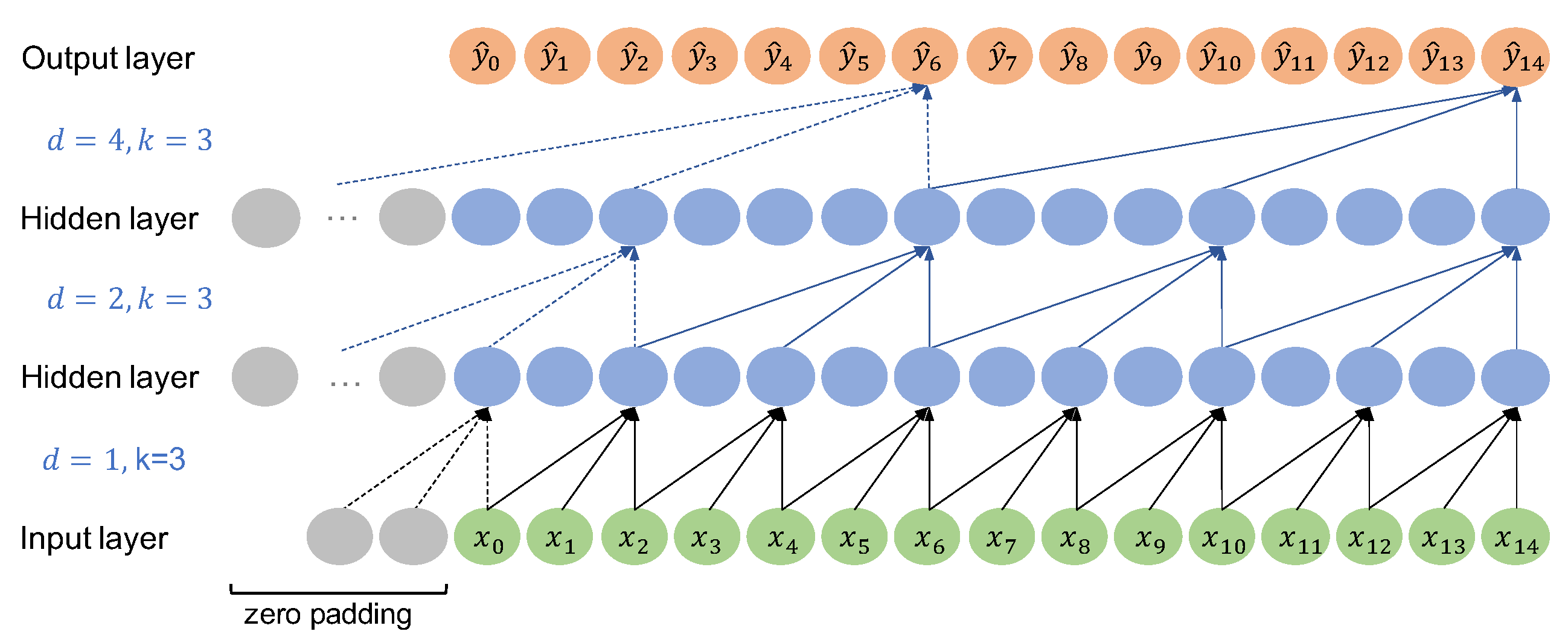
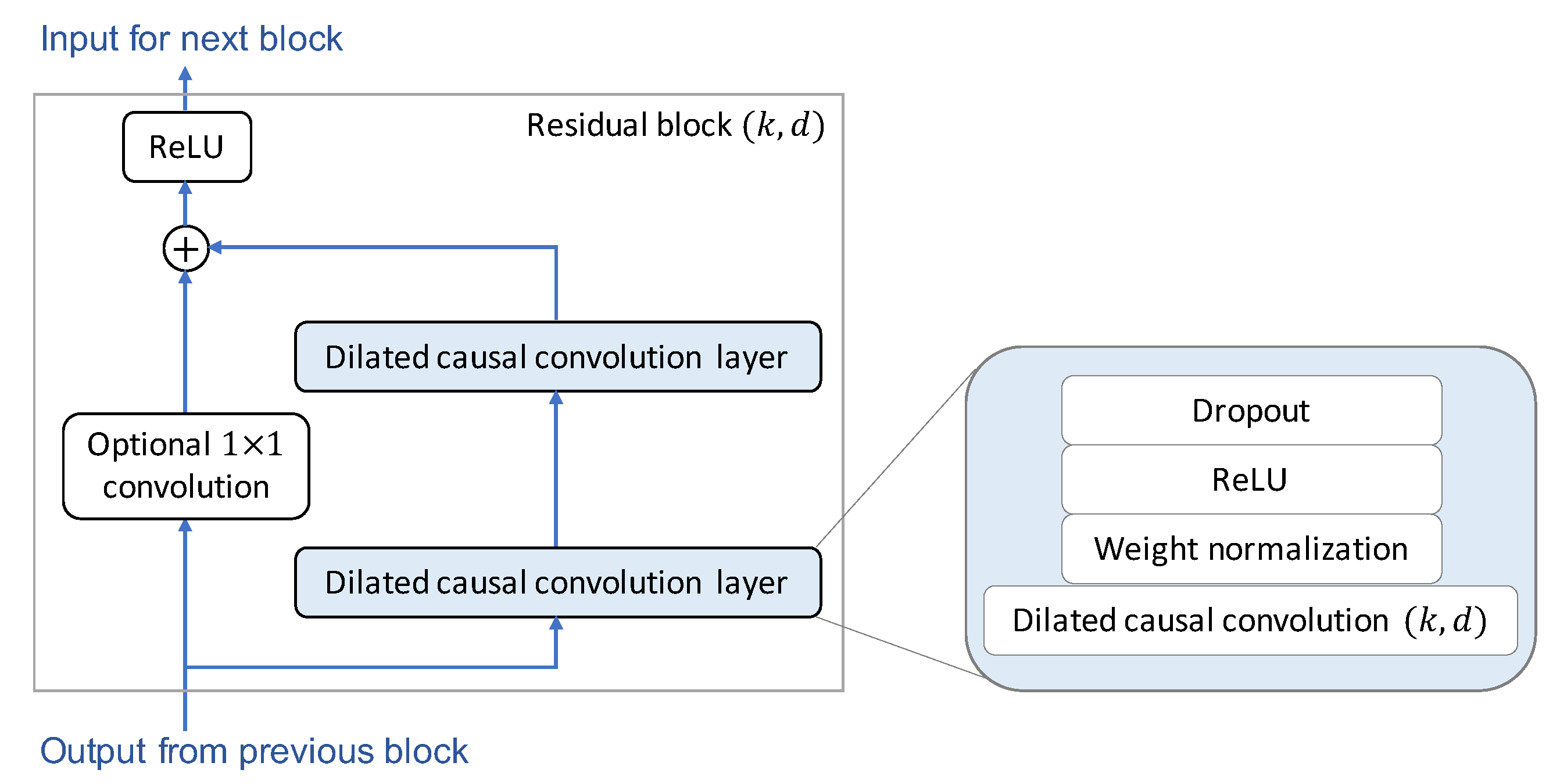
3.3. TCN
4. Method
4.1. The Framework for Predicting Monthly Average of TAIEX
4.1.1. Identifying Potential Factors
4.1.2. Data Preprocessing
- Handling missing values: When collecting daily financial and economic factors representing global stock markets, some missing values occurred in the dataset due to the different holidays in each country or region. Since there are only a few missing values in the dataset, we adopted a simple solution to this problem: to fill the missing value with the value of the preceding trading day.
- Identifying the most valuable features: To select the most relevant independent variables from all candidates, we evaluated the pairwise correlation between each variable and the target variable TAIEX, and then picked out only those with a high correlation value. Correlation reflects the degree to which two variables are linearly associated, and the value is usually in the range of . The positive or negative sign indicates whether two variables are positively or negatively related, and or 1 means that two variables have a perfect negative or positive correlation. We used Spearman’s rank correlation coefficient to measure the correlation. Compared to another well-known correlation coefficient, Pearson’s coefficient, which only works with a linear relationship between two variables, Spearman’s coefficient can also work with monotonic relationships. In addition, the Spearman correlation is less sensitive to outliers than the Pearson correlation. The optimized subset of features may differ for each forecast distance s; therefore, we calculated the pairwise correlation for each case of s. In this way, the time interval between any pair of values of the independent variable and the target variable in the calculation of correlation was defined by , where 22 is the average number of regular trading days in a month for a stock market. In addition to the correlation coefficient, we also performed a hypothesis test of the “significance of the correlation coefficient” to ensure that the linear relationship in the sample data was strong enough to reflect the actual relationship in the whole population. Any feature having the significance of the correlation coefficient () less than the significance level would not be selected.
- Feature transformation: We applied two well-known feature transformation techniques to enhance the framework’s performance. The first technique is standardization, a feature scaling method that allows normalizing the range of values of independent variables. Through standardization, the values of each variable have a zero mean and unit variance. The second technique is Principal Component Analysis (PCA), a popular method for dimensionality reduction. Many studies have shown that using PCA can improve the performance of stock prediction models in terms of accuracy and stability [10,18,47,48]. PCA helps preserve only the majority of the variance (information); hence the complexity of the models and the training time can be significantly reduced. Moreover, by reducing the complexity, the overfitting problem can also be prevented to a certain extent. Our framework tried to select the number of components n so that the amount of variance they can explain is at least 95% of the total variance.
4.1.3. Training Models
- Hyperparameter tuning: We split the available data into a training set and a validation set . The data from year backward are used for , while the data from year are used for to tune two hyperparameters: the batch size used in the Stochastic Gradient Descent and the sequence length .
- Training final model: The framework retrains the models using all available data () and the optimal hyperparameters found in the previous phase. These models are the final models that will be used to predict MATs in year Y.
4.2. Simulated Trading
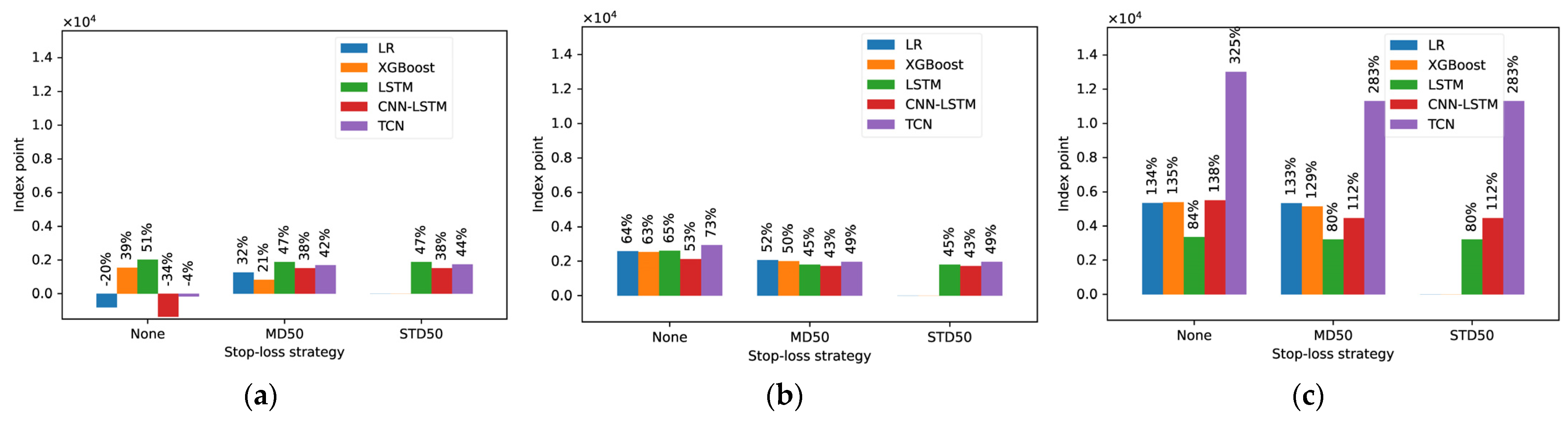
- Manual Determination (MD strategy): Individual investors can define the threshold based on their bearable loss, i.e., if the investor can afford a loss , he can hold their long position in an MTX contract until its value falls to the stop-loss threshold , where is the value of the contract at the time the investor owns the contract.
- Inferring from the predicted Standard Deviation (STD strategy): Since the contract’s value can fluctuate for a while before reaching our predicted value, we do not want to abandon a contract too early due to a temporary drop in a “normal” range. We have proposed to take the predicted standard deviation of the daily predicted contract’s values to determine the normal range for the target month. In this way, we allow the value to fall up to (), where is the predicted MAT value and is calculated from the models’ 22 output values for the target month. In conjunction with the affordable loss concept mentioned earlier, we suggested to compute the stop-loss threshold as .
5. Empirical Results
5.1. Data Specification
5.2. Models Setting
- Hyperparameters related to specific network structure
- (a)
- LSTM:
- Number of LSTM layers: 2
- Number of neurons in hidden layer: 200
- Dropout probability: 0.3 (using dropout between LSTM layers and before passing the output of the final LSTM layer to the FC layer to reduce overfitting. A good value for dropout probability is between 0.3 and 0.9 [46]. We selected 0.3, since the number of neurons in the hidden layer is not much.)
- (b)
- CNN-LSTM:
- For CNN network:
- -
- Number of 1D convolution layers: 1
- -
- Out channels of 1D convolution layer:
- -
- Kernel size 5 and stride 5
- For LSTM network: same as the above LSTM network.
- (c)
- TCN:
- Number of residual blocks (TCN networks require a minimum number of residual blocks, which depends on the sequence length, for full history coverage):
- Kernel size 3 and stride 1
- Dilation factor: for residual block
- Out channels of the dilated causal convolutions: 22
- Dropout probability: 0.3
- General training hyperparameters
- Input sequence length : (these values correspond to the number of trading days in 6, 12, 18, 24, 30, and 36 months, respectively).
- Batch size :
- Optimizer: Adam
- -
- Learning rate:
- -
- -
- -
- Weight decay:
- Loss function: Mean squared error
- Max Epochs: 100
- Early training-stopped condition: No further improvement on the loss of validation data over 10 consecutive epochs.
5.3. Evaluation
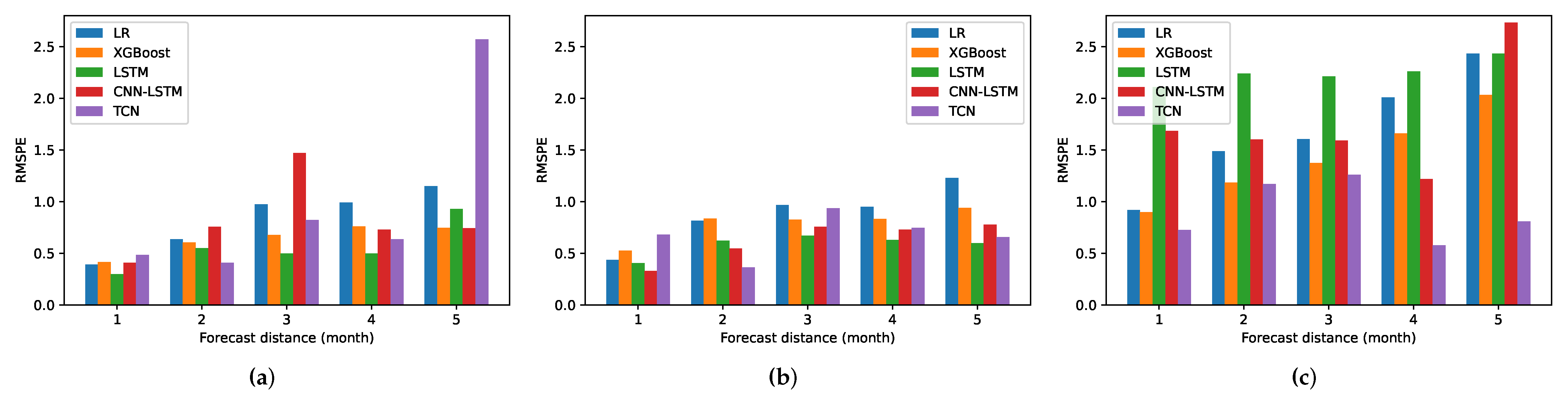
5.3.1. RMSPE
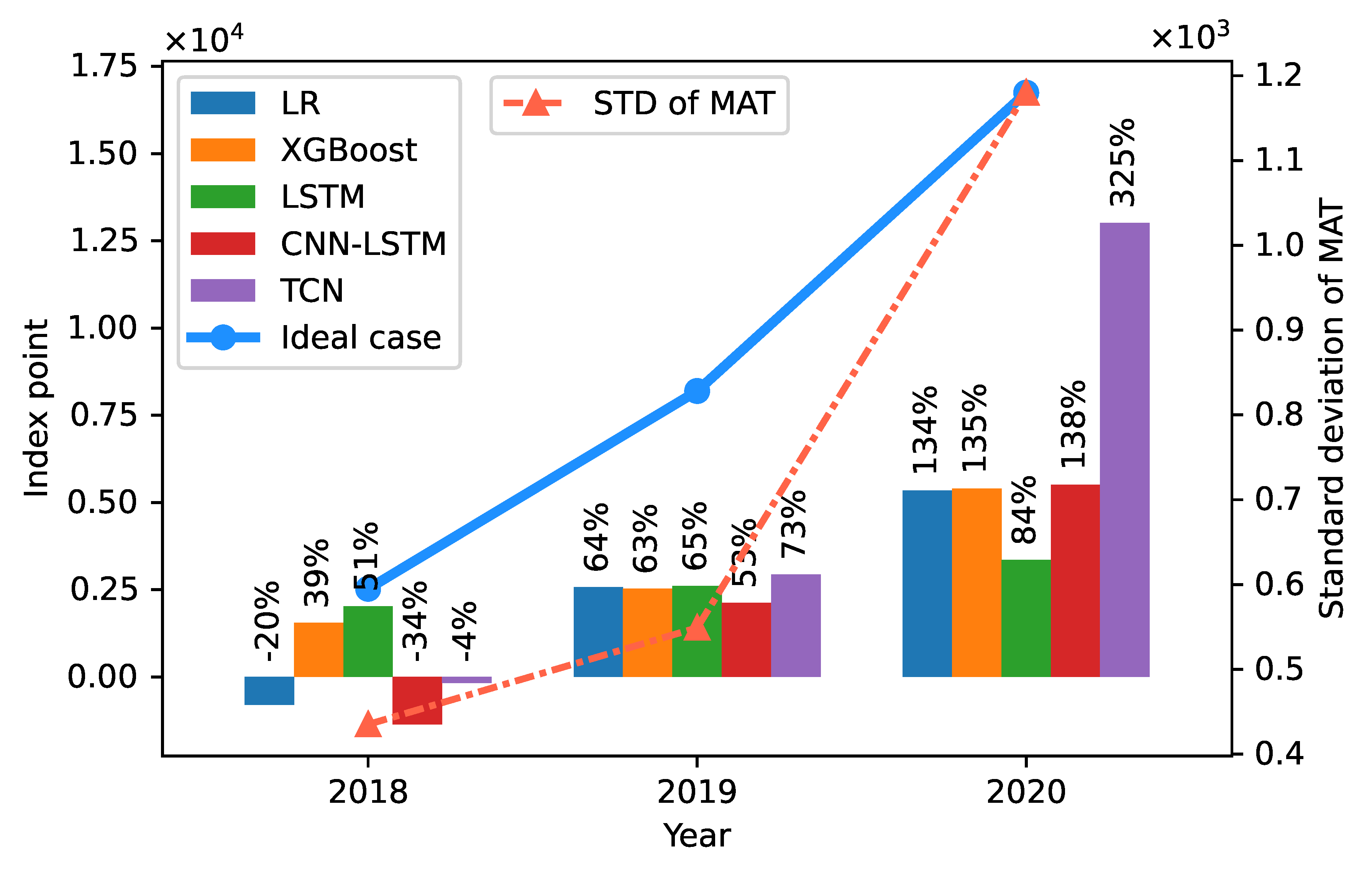
5.3.2. Profit
6. Conclusions
Author Contributions
Funding
Institutional Review Board Statement
Informed Consent Statement
Data Availability Statement
Conflicts of Interest
Appendix A

| # | Variable | Symbol | Description | Types |
|---|---|---|---|---|
| 1 | AORD | ^AORD | ALL ORDINARIES | World Indices |
| 2 | AXJO | ^AXJO | S&P/ASX 200 | World Indices |
| 3 | N225 | ^N225 | Nikkei 225 | World Indices |
| 4 | KOSPI | ^KS11 | KOSPI Composite Index | World Indices |
| 5 | SSE | 000001.SS | SSE Composite Index | World Indices |
| 6 | SSEA | 000002.SS | SSE A Share Index | World Indices |
| 7 | SZSE | 399001.SZ | Shenzhen Component | World Indices |
| 8 | HSI | ^HSI | HANG SENG INDEX | World Indices |
| 9 | KLSE | ^KLSE | FTSE Bursa Malaysia KLCI | World Indices |
| 10 | STI | ^STI | STI Index | World Indices |
| 11 | PSEI | PSEI.PS | PSEi INDEX | World Indices |
| 12 | JKSE | ^JKSE | Jakarta Composite Index | World Indices |
| 13 | BSESN | ^BSESN | S&P BSE SENSEX | World Indices |
| 14 | FTSE | ^FTSE | FTSE 100 | World Indices |
| 15 | GDAXI | ^GDAXI | DAX PERFORMANCE-INDEX | World Indices |
| 16 | FCHI | ^FCHI | CAC40 | World Indices |
| 17 | SSMI | ^SSMI | SMI PR | World Indices |
| 18 | DJI | ^DJI | Dow Jones Industrial Average | World Indices |
| 19 | GSPC | ^GSPC | S&P 500 | World Indices |
| 20 | IXIC | ^IXIC | NASDAQ Composite | World Indices |
| 21 | SOX | ^SOX | PHLX Semiconductor | World Indices |
| 22 | GSPTSE | ^GSPTSE | S&P/TSX Composite index | World Indices |
| 23 | MXX | ^MXX | IPC MEXICO | World Indices |
| 24 | BVSP | ^BVSP | IBOVESPA | World Indices |
| 25 | VIX | ^VIX | CBOE Volatility Index | World Indices |
| 26 | IRX | ^IRX | 13 Week Treasury Bill | US Treasury bonds rates |
| 27 | TYX | ^TYX | Treasury Yield 30 Years | US Treasury bonds rates |
| 28 | FVX | ^FVX | Treasury Yield 5 Years | US Treasury bonds rates |
| 29 | TNX | ^TNX | Treasury Yield 10 Years | US Treasury bonds rates |
| 30 | TSM | TSM | Taiwan Semiconductor Manufacturing Company Limited | Taiwan Company |
| 31 | MSCI | MSCI | MSCI Inc. | U.S. Company |
| 32 | CrudeOil | CL=F | Crude Oil May 21 | Commodity |
| 33 | HeatingOil | HO=F | Heating Oil May 21 | Commodity |
| 34 | NaturalGas | NG=F | Natural Gas May 21 | Commodity |
| 35 | Gold | GC=F | Gold Jun 21 | Commodity |
| 36 | Platinum | PL=F | Platinum Jul 21 | Commodity |
| 37 | Silver | SI=F | Silver May 21 | Commodity |
| 38 | Copper | HG=F | Copper May 21 | Commodity |
| 39 | Palladium | PA=F | Palladium Jun 21 | Commodity |
| 40 | TWDUSD | TWDUSD=X | TWD/USD exchange rates | TWD exchange rates |
| 41 | TWDCNY | TWDCNY=X | TWD/CNY exchange rates | TWD exchange rates |
| 42 | TWDJPY | TWDJPY=X | TWD/JPY exchange rates | TWD exchange rates |
| 43 | TWDHKD | TWDHKD=X | TWD/HKD exchange rates | TWD exchange rates |
| 44 | TWDKRW | TWDKRW=X | TWD/KRW exchange rates | TWD exchange rates |
| 45 | TWDEUR | TWDEUR=X | TWD/EUR exchange rates | TWD exchange rates |
| 46 | TWDCAD | TWDCAD=X | TWD/CAD exchange rates | TWD exchange rates |
| Year | None | MD50 | STD50 |
|---|---|---|---|
| 2018 | 2525 | 2352 | 2525 |
| 2019 | 8196 | 5157 | 6496 |
| 2020 | 16,746 | 12,084 | 12,084 |
| Year | # | LSTM | CNN-LSTM | TCN | |||||||||
| 2018 | 1 | 10,840 | 10,556 | 50 | - | 11,417 | 10,535 | 50 | - | 10,612 | 10,535 | 50 | - |
| 2 | 10,914 | 10,557 | 50 | - | 10,813 | 10,557 | 50 | - | 12,001 | 11,012 | 50 | 873 | |
| 3 | 10,792 | 10,849 | 107 | 17 | 11,758 | 10,809 | 50 | 380 | 10,028 | 10,551 | 573 | - | |
| 4 | 11,100 | 10,118 | 50 | - | 10,833 | 10,577 | 50 | 126 | 10,811 | 10,809 | 50 | 380 | |
| 5 | 10,795 | 10,545 | 50 | - | 10,883 | 10,373 | 50 | - | 12,818 | 10,118 | 50 | - | |
| 6 | 10,668 | 10,495 | 50 | - | 11,878 | 10,450 | 50 | - | 9850 | 10,545 | 745 | - | |
| 7 | 11,212 | 10,885 | 50 | 329 | 11,872 | 10,920 | 50 | 1229 | 10,605 | 10,450 | 50 | - | |
| 8 | 10,301 | 9692 | 50 | 126 | 11,959 | 10,935 | 50 | 1584 | 12,291 | 10,885 | 50 | 1534 | |
| 9 | 10,170 | 9951 | 50 | 375 | 11,967 | 10,889 | 50 | 1538 | 10,930 | 10,889 | 50 | 1538 | |
| 10 | 10,762 | 9692 | 50 | 126 | 9412 | 9699 | 337 | 133 | |||||
| 11 | 10,171 | 9951 | 50 | 375 | |||||||||
| 2019 | 1 | 9932 | 9657 | 50 | 388 | 9866 | 9657 | 50 | 388 | 9676 | 9657 | 50 | 388 |
| 2 | 10,573 | 9895 | 50 | - | 10,003 | 9895 | 50 | - | 10,389 | 9895 | 50 | - | |
| 3 | 10,617 | 10,336 | 50 | 182 | 10,906 | 10,336 | 50 | 182 | 10,029 | 10,145 | 166 | - | |
| 4 | 10,576 | 10,613 | 87 | 36 | 11,043 | 10,627 | 50 | 50 | 10,447 | 10,519 | 122 | - | |
| 5 | 10,530 | 9978 | 50 | - | 11,069 | 10,895 | 50 | 603 | 10,606 | 10,551 | 50 | 421 | |
| 6 | 10,627 | 10,475 | 50 | - | 10,559 | 10,145 | 50 | - | 10,318 | 10,482 | 214 | - | |
| 7 | 10,806 | 10,500 | 50 | - | 10,852 | 10,655 | 50 | - | 10,530 | 10,778 | 298 | - | |
| 8 | 10,253 | 10,482 | 279 | - | 11,085 | 10,583 | 50 | 453 | |||||
| 9 | 10,737 | 10,516 | 50 | 9 | |||||||||
| 10 | 10,939 | 10,800 | 50 | 41 | |||||||||
| 2020 | 1 | 11,343 | 11,236 | 50 | 148 | 11,465 | 11,236 | 50 | 148 | 12,882 | 11,164 | 50 | 2690 |
| 2 | 10,924 | 10,950 | 76 | - | 11,987 | 10,908 | 50 | 2434 | 11,944 | 10,960 | 50 | 2486 | |
| 3 | 8672 | 9401 | 779 | - | 10,413 | 9401 | 50 | - | 13,002 | 9401 | 50 | - | |
| 4 | 9641 | 10,058 | 467 | - | 10,327 | 10,276 | 50 | - | 13,725 | 10,276 | 50 | - | |
| 5 | 10,209 | 10,564 | 405 | - | 12,168 | 10,564 | 50 | - | 13,954 | 10,635 | 50 | - | |
| 6 | 13,985 | 11,206 | 50 | - | |||||||||
| 7 | 14,786 | 12,358 | 50 | 263 | |||||||||
| 8 | 15,114 | 12,444 | 50 | 344 | |||||||||
| 9 | 15,451 | 12,421 | 50 | - | |||||||||
| 10 | 13,967 | 12,357 | 50 | - | |||||||||
References
- Gandhmal, D.P.; Kumar, K. Systematic analysis and review of stock market prediction techniques. Comput. Sci. Rev. 2019, 34, 1–13. [Google Scholar] [CrossRef]
- Henrique, B.M.; Sobreiro, V.A.; Kimura, H. Literature review: Machine learning techniques applied to financial market prediction. Expert Syst. Appl. 2019, 124, 226–251. [Google Scholar] [CrossRef]
- Kumar, G.; Jain, S.; Singh, U.P. Stock Market Forecasting Using Computational Intelligence: A Survey. Arch. Comput. Methods Eng. 2021, 28, 1069–1101. [Google Scholar] [CrossRef]
- Fama, E.F. Random Walks in Stock Market Prices. Financ. Anal. J. 1995, 51, 75–80. [Google Scholar] [CrossRef] [Green Version]
- Sezer, O.B.; Gudelek, M.U.; Ozbayoglu, A.M. Financial time series forecasting with deep learning: A systematic literature review: 2005–2019. Appl. Soft Comput. 2020, 90, 106181. [Google Scholar] [CrossRef] [Green Version]
- Bustos, O.; Pomares-Quimbaya, A. Stock market movement forecast: A Systematic review. Expert Syst. Appl. 2020, 156, 113464. [Google Scholar] [CrossRef]
- Weng, B.; Ahmed, M.A.; Megahed, F.M. Stock market one-day ahead movement prediction using disparate data sources. Expert Syst. Appl. 2017, 79, 153–163. [Google Scholar] [CrossRef]
- Wang, J.; Wang, J.; Fang, W.; Niu, H. Financial Time Series Prediction Using Elman Recurrent Random Neural Networks. Comput. Intell. Neurosci. 2016, 2016, 1–14. [Google Scholar] [CrossRef] [Green Version]
- Persio, L.D.; Honchar, O. Artificial Neural Networks architectures for stock price prediction: Comparisons and applications. Int. J. Circuits Syst. Signal Process. 2016, 10, 403–413. [Google Scholar]
- Chong, E.; Han, C.; Park, F.C. Deep learning networks for stock market analysis and prediction: Methodology, data representations, and case studies. Expert Syst. Appl. 2017, 83, 187–205. [Google Scholar] [CrossRef] [Green Version]
- Gunduz, H.; Yaslan, Y.; Cataltepe, Z. Intraday prediction of Borsa Istanbul using convolutional neural networks and feature correlations. Knowl.-Based Syst. 2017, 137, 138–148. [Google Scholar] [CrossRef]
- Li, Z.; Tam, V. Combining the real-time wavelet denoising and long-short-term-memory neural network for predicting stock indexes. In Proceedings of the 2017 IEEE Symposium Series on Computational Intelligence (SSCI), Honolulu, HI, USA, 27 November–1 December 2017; pp. 1–8. [Google Scholar]
- Fischer, T.; Krauss, C. Deep learning with long short-term memory networks for financial market predictions. Eur. J. Oper. Res. 2018, 270, 654–669. [Google Scholar] [CrossRef] [Green Version]
- Baek, Y.; Kim, H.Y. ModAugNet: A new forecasting framework for stock market index value with an overfitting prevention LSTM module and a prediction LSTM module. Expert Syst. Appl. 2018, 113, 457–480. [Google Scholar] [CrossRef]
- Chung, H.; Shin, K.s. Genetic Algorithm-Optimized Long Short-Term Memory Network for Stock Market Prediction. Sustainability 2018, 10, 3765. [Google Scholar] [CrossRef] [Green Version]
- Chen, L.; Qiao, Z.; Wang, M.; Wang, C.; Du, R.; Stanley, H.E. Which Artificial Intelligence Algorithm Better Predicts the Chinese Stock Market? IEEE Access 2018, 6, 48625–48633. [Google Scholar] [CrossRef]
- Zhou, X.; Pan, Z.; Hu, G.; Tang, S.; Zhao, C. Stock Market Prediction on High-Frequency Data Using Generative Adversarial Nets. Math. Probl. Eng. 2018, 2018, 4907423. [Google Scholar] [CrossRef] [Green Version]
- Zhong, X.; Enke, D. Predicting the daily return direction of the stock market using hybrid machine learning algorithms. Financ. Innov. 2019, 5, 1–20. [Google Scholar] [CrossRef]
- Hoseinzade, E.; Haratizadeh, S. CNNpred: CNN-based stock market prediction using a diverse set of variables. Expert Syst. Appl. 2019, 129, 273–285. [Google Scholar] [CrossRef]
- Sim, H.S.; Kim, H.I.; Ahn, J.J. Is Deep Learning for Image Recognition Applicable to Stock Market Prediction? Complexity 2019, 2019, 4324878. [Google Scholar] [CrossRef]
- Wen, M.; Li, P.; Zhang, L.; Chen, Y. Stock Market Trend Prediction Using High-Order Information of Time Series. IEEE Access 2019, 7, 28299–28308. [Google Scholar] [CrossRef]
- Lee, J.; Kim, R.; Koh, Y.; Kang, J. Global Stock Market Prediction Based on Stock Chart Images Using Deep Q-Network. IEEE Access 2019, 7, 167260–167277. [Google Scholar] [CrossRef]
- Long, W.; Lu, Z.; Cui, L. Deep learning-based feature engineering for stock price movement prediction. Knowl.-Based Syst. 2019, 164, 163–173. [Google Scholar] [CrossRef]
- Pang, X.; Zhou, Y.; Wang, P.; Lin, W.; Chang, V. An innovative neural network approach for stock market prediction. J. Supercomput. 2020, 76, 2098–2118. [Google Scholar] [CrossRef]
- Kelotra, A.; Pandey, P. Stock Market Prediction Using Optimized Deep-ConvLSTM Model. Big Data 2020, 8, 5–24. [Google Scholar] [CrossRef] [PubMed] [Green Version]
- Chung, H.; Shin, K.s. Genetic algorithm-optimized multi-channel convolutional neural network for stock market prediction. Neural Comput. Appl. 2020, 32, 7897–7914. [Google Scholar] [CrossRef]
- Nabipour, M.; Nayyeri, P.; Jabani, H.; Mosavi, A.; Salwana, E.; Shahab, S. Deep learning for stock market prediction. Entropy 2020, 22, 840. [Google Scholar] [CrossRef]
- Long, J.; Chen, Z.; He, W.; Wu, T.; Ren, J. An integrated framework of deep learning and knowledge graph for prediction of stock price trend: An application in Chinese stock exchange market. Appl. Soft Comput. 2020, 91, 106205. [Google Scholar] [CrossRef]
- Nabipour, M.; Nayyeri, P.; Jabani, H.; Shahab, S.; Mosavi, A. Predicting Stock Market Trends Using Machine Learning and Deep Learning Algorithms Via Continuous and Binary Data; a Comparative Analysis. IEEE Access 2020, 8, 150199–150212. [Google Scholar] [CrossRef]
- Lei, B.; Zhang, B.; Song, Y. Volatility Forecasting for High-Frequency Financial Data Based on Web Search Index and Deep Learning Model. Mathematics 2021, 9, 320. [Google Scholar] [CrossRef]
- Hsieh, T.J.; Hsiao, H.F.; Yeh, W.C. Forecasting stock markets using wavelet transforms and recurrent neural networks: An integrated system based on artificial bee colony algorithm. Appl. Soft Comput. 2011, 11, 2510–2525. [Google Scholar] [CrossRef]
- Sun, W.T.; Chiao, H.T.; Chang, Y.S.; Yuan, S.M. Forecasting Monthly Average of Taiwan Stock Exchange Index. In New Trends in Computer Technologies and Applications; Springer: Singapore, 2019; pp. 302–309. [Google Scholar]
- Ha, D.A.; Lu, J.D.; Yuan, S.M. Forecasting Taiwan StocksWeighted Index Monthly Average Based on Linear Regression—Applied to Taiwan Stock Index Futures. In Education and Awareness of Sustainability; World Scientific: Singapore, 2020; pp. 431–435. [Google Scholar]
- Tan, K.S.; Lio, C.H.; Yuan, S.M. Futures Trading Strategy based on Monthly Average Prediction of TAIEX by using Linear Regression and XGBoost. In Proceedings of the 7th IEEE International Conference on Applied System Innovation 2021, Alishan, Taiwan, 24–25 September 2021. [Google Scholar]
- Hochreiter, S.; Schmidhuber, J. Long Short-Term Memory. Neural Comput. 1997, 9, 1735–1780. [Google Scholar] [CrossRef] [PubMed]
- Olah, C. Understanding LSTM Networks. Available online: http://colah.github.io/posts/2015-08-Understanding-LSTMs/ (accessed on 30 September 2021).
- Chevalier, G. LSTM Cell. Available online: https://commons.wikimedia.org/wiki/File:LSTM_Cell.svg (accessed on 30 September 2021).
- Shi, X.; Chen, Z.; Wang, H.; Yeung, D.Y.; Wong, W.K.; Woo, W.C. Convolutional LSTM Network: A Machine Learning Approach for Precipitation Nowcasting. arXiv 2015, arXiv:cs.CV/1506.04214. [Google Scholar]
- Sainath, T.N.; Vinyals, O.; Senior, A.; Sak, H. Convolutional, Long Short-Term Memory, fully connected Deep Neural Networks. In Proceedings of the 2015 IEEE International Conference on Acoustics, Speech and Signal Processing (ICASSP), South Brisbane, Australia, 19–24 April 2015; pp. 4580–4584. [Google Scholar]
- Donahue, J.; Hendricks, L.A.; Rohrbach, M.; Venugopalan, S.; Guadarrama, S.; Saenko, K.; Darrell, T. Long-term Recurrent Convolutional Networks for Visual Recognition and Description. arXiv 2016, arXiv:cs.CV/1411.4389. [Google Scholar]
- Livieris, I.E.; Pintelas, E.; Pintelas, P. A CNN-LSTM model for gold price time-series forecasting. Neural Comput. Appl. 2020, 32, 17351–17360. [Google Scholar] [CrossRef]
- Bai, S.; Kolter, J.Z.; Koltun, V. An Empirical Evaluation of Generic Convolutional and Recurrent Networks for Sequence Modeling. arXiv 2018, arXiv:cs.LG/1803.01271. [Google Scholar]
- Long, J.; Shelhamer, E.; Darrell, T. Fully convolutional networks for semantic segmentation. In Proceedings of the 2015 IEEE Conference on Computer Vision and Pattern Recognition (CVPR), Boston, MA, USA, 7–12 June 2015; pp. 3431–3440. [Google Scholar]
- He, K.; Zhang, X.; Ren, S.; Sun, J. Deep Residual Learning for Image Recognition. In Proceedings of the 2016 IEEE Conference on Computer Vision and Pattern Recognition (CVPR), Las Vegas, NV, USA, 27–30 June 2016; pp. 770–778. [Google Scholar]
- Salimans, T.; Kingma, D.P. Weight Normalization: A Simple Reparameterization to Accelerate Training of Deep Neural Networks. In Proceedings of the 30th International Conference on Neural Information Processing Systems, Barcelona, Spain, 5–10 December 2016; pp. 901–909. [Google Scholar]
- Srivastava, N.; Hinton, G.; Krizhevsky, A.; Sutskever, I.; Salakhutdinov, R. Dropout: A Simple Way to Prevent Neural Networks from Overfitting. J. Mach. Learn. Res. 2014, 15, 1929–1958. [Google Scholar]
- Zhong, X.; Enke, D. Forecasting daily stock market return using dimensionality reduction. Expert Syst. Appl. 2017, 67, 126–139. [Google Scholar] [CrossRef]
- Weng, B.; Lu, L.; Wang, X.; Megahed, F.M.; Martinez, W. Predicting short-term stock prices using ensemble methods and online data sources. Expert Syst. Appl. 2018, 112, 258–273. [Google Scholar] [CrossRef]
- Ismail Fawaz, H.; Lucas, B.; Forestier, G.; Pelletier, C.; Schmidt, D.F.; Weber, J.; Webb, G.I.; Idoumghar, L.; Muller, P.A.; Petitjean, F. InceptionTime: Finding AlexNet for time series classification. Data Min. Knowl. Discov. 2020, 34, 1936–1962. [Google Scholar] [CrossRef]
- Dempster, A.; Petitjean, F.; Webb, G.I. ROCKET: Exceptionally fast and accurate time series classification using random convolutional kernels. Data Min. Knowl. Discov. 2020, 34, 1454–1495. [Google Scholar] [CrossRef]


| Article | Target Data | Input Variables | Target Output | Main Method | Simulated Trading | Year |
|---|---|---|---|---|---|---|
| Wang et al. [8] | SSE, TAIEX, KOSPI, and NIKKEI | Stock prices | Price; Daily | RNN | N | 2016 |
| Persio and Honchar [9] | S&P 500 | Stock prices | Direction; Daily | MLP, RNN, CNN | N | 2016 |
| Chong et al. [10] | KOSPI 38 stock returns | Intraday stock returns | Return; 5 min ahead | DNN | N | 2017 |
| Gunduz et al. [11] | Borsa Istabul BIST 100 stocks | Technical indicators, stock prices, temporal variable | Direction; hourly | CNN | N | 2017 |
| Li and Tam [12] | HIS, SSE, SZSE, TAIEX, NIKKEI, KOSPI | Technical indicators, stock prices | Price; Daily | LSTM | N | 2017 |
| Fischer and Krauss [13] | S&P 500 | Stock prices | Direction; Daily | LSTM | N | 2018 |
| Baek and Kim [14] | S&P 500, KOSPI | Stock prices | Price; Daily | LSTM | Y | 2018 |
| Chung and Shin [15] | KOSPI | Technical indicators, stock prices | Price; Daily | LSTM | N | 2018 |
| Chen et al. [16] | CSI 300 futures contract | Transaction data | Price; 1 min ahead | DNN | N | 2018 |
| Zhou et al. [17] | Stocks in CSI 300 | Technical indicators | Price; 1 min ahead | GAN based on LSTM and CNN | N | 2018 |
| Zhong and Enke [18] | SPY | Technical indicators, financial and economic factors | Direction; Daily | DNN, ANN | Y | 2019 |
| Hoseinzade and Haratizadeh [19] | S&P 500, NASDAQ, DJI, NYSE, and RUSSELL | Technical indicators, stock prices, financial and economic factors | Direction; Daily | CNN | N | 2019 |
| Sim et al. [20] | S&P 500 | Technical indicators | Direction; 1 min ahead | CNN | N | 2019 |
| Wen et al. [21] | S&P 500 and its individual stocks | Stock prices | Price; Daily | CNN | N | 2019 |
| Lee et al. [22] | US stocks | Stock chart images of daily closing price and volume data | Return; Daily | CNN | N | 2019 |
| Long et al. [23] | CSI 300 | Stock prices | Direction; 5–30 min ahead | MFNN based on CNN and LSTM | Y | 2019 |
| Pang et al. [24] | Shanghai A-share composite index, and 3 stocks | Technical indicators, stock prices | Price; Daily | LSTM | N | 2020 |
| Kelotra and Fiaz [25] | 6 stocks | Technical indicators | Price; Daily | ConvLSTM | N | 2020 |
| Chung and Shin [26] | KOSPI | Technical indicators | Direction; Daily | CNN | N | 2020 |
| Nabipour et al. [27] | 4 stock market groups | Technical indicators | Price; 1–30 days ahead | ANN, RNN, LSTM | N | 2020 |
| Long et al. [28] | CITIC Securities, GF Securities, China Pingan | Transaction records data and public market information | Direction; 1 day ahead for stock price movement; 5- and 7-days trend | DSPNN based on CNN and LSTM | N | 2020 |
| Nabipour et al. [29] | 4 stock market groups | Technical indicators | Direction; Daily | RNN, LSTM, DT, RF, Adaboost, XGBoost, SVC, NB, KNN, LR, ANN | N | 2020 |
| Lei et al. [30] | SSE | Technical indicators, stock prices, investor attention factor synthesized by Baidu search index | Volatility; Daily | TCN | N | 2021 |
| Type of Feature Set | # of Features | # of Selected Features for Each Forecast Distance | |
|---|---|---|---|
| {1, 2, 4} | {3, 5} | ||
| World Indices | 25 | 20 | 19 |
| US Treasury bonds rates | 4 | 0 | 0 |
| Commodity | 8 | 1 | 1 |
| TWD exchange rates | 7 | 2 | 2 |
| Companies | 2 | 2 | 2 |
| Total | 46 | 25 | 24 |
| LR | XGBoost | CNN-LSTM | LSTM | TCN | |
|---|---|---|---|---|---|
| In top one model | 0 | 0 | 2 | 6 | 7 |
| In top two models | 1 | 6 | 6 | 8 | 9 |
Publisher’s Note: MDPI stays neutral with regard to jurisdictional claims in published maps and institutional affiliations. |
© 2021 by the authors. Licensee MDPI, Basel, Switzerland. This article is an open access article distributed under the terms and conditions of the Creative Commons Attribution (CC BY) license (https://creativecommons.org/licenses/by/4.0/).
Share and Cite
Ha, D.-A.; Liao, C.-H.; Tan, K.-S.; Yuan, S.-M. Deep Learning Models for Predicting Monthly TAIEX to Support Making Decisions in Index Futures Trading. Mathematics 2021, 9, 3268. https://doi.org/10.3390/math9243268
Ha D-A, Liao C-H, Tan K-S, Yuan S-M. Deep Learning Models for Predicting Monthly TAIEX to Support Making Decisions in Index Futures Trading. Mathematics. 2021; 9(24):3268. https://doi.org/10.3390/math9243268
Chicago/Turabian StyleHa, Duy-An, Chia-Hung Liao, Kai-Shien Tan, and Shyan-Ming Yuan. 2021. "Deep Learning Models for Predicting Monthly TAIEX to Support Making Decisions in Index Futures Trading" Mathematics 9, no. 24: 3268. https://doi.org/10.3390/math9243268
APA StyleHa, D.-A., Liao, C.-H., Tan, K.-S., & Yuan, S.-M. (2021). Deep Learning Models for Predicting Monthly TAIEX to Support Making Decisions in Index Futures Trading. Mathematics, 9(24), 3268. https://doi.org/10.3390/math9243268