Novel Analytical Approach for the Space-Time Fractional (2+1)-Dimensional Breaking Soliton Equation via Mathematical Methods

Abstract

The aim of this work is to build novel analytical wave solutions of the nonlinear space-time fractional (2+1)-dimensional breaking soliton equations, with regards to the modified Riemann–Liouville derivative, by employing mathematical schemes, namely, the improved simple equation and modified F-expansion methods. We used the fractional complex transformation of the concern fractional differential equation to convert it for the solvable integer order differential equation. After the successful implementation of the presented methods, a comprehensive class of novel and broad-ranging exact and solitary travelling wave solutions were discovered, in terms of trigonometric, rational and hyperbolic functions. Hence, the present methods are reliable and efficient for solving nonlinear fractional problems in mathematics physics.

1. Introduction

The fractional order of nonlinear partial differential equations (NPDEs) arise in numerous grounds like the theoretical physics, dynamical system, fluid dynamics, elasticity, gas dynamics, plasma physics, solid state physics, MHD and many others. The construction of the exact solutions is one of the dominant leitmotifs in applied mathematics and theoretical physics. Moreover, the fractional order in calculus is one the developing fields of applied mathematics and physics and whose idea was first instigated with the possibility of fractional derivatives by Leibniz in 1695 [1]. Liouville laid the basic rules of this subject in (1832) and Riemann discovered the fractional derivative of a power function Riemann in (1847) [2]. The plethora of attention has been received to determine the incipient and closed form exact solutions of FPDEs by many researchers. The potential symbolic computer programming implements have been utilized to investigate opportune solutions to NFPDEs, namely, first integral method [3,4,5], modified simple equation schemes [6,7], dirct agebric methods and auxiliary equation techniques [8,9,10], fractional equation scheme [11,12,13,14], $(G^{\prime }/G)$ -expansion scheme [15,16,17], Lie-symmetry technique [18], Seadawy and Exp function methods [19,20,21,22], tanh-coth scheme [23], generalized Kudryashov scheme [24,25,26,27,28,29] and many more [30,31,32,33,34,35,36,37,38].

Let the time fractional breaking soliton model be stated as in [39]:

$$\begin{array}{c}\frac{{\partial }^{\alpha }U}{\partial t^{\alpha }}+a\frac{{\partial }^{3\alpha }U}{\partial x^{2\alpha }{y}^{\alpha }}+4aU\frac{{\partial }^{\alpha }V}{\partial x^{\alpha }}+4a\frac{{\partial }^{\alpha }U}{\partial x^{\alpha }}V=0,\hfill \\ \frac{{\partial }^{\alpha }U}{\partial y^{\alpha }}-\frac{{\partial }^{\alpha }V}{\partial x^{\alpha }}=0,0<\alpha \le 1.\hfill \end{array}$$

(1)

Currently different schemes to find solutions of Equation (1) have been presented. Yildirim and Yasar discussed a wave solution of the (2+1)-dimensional breaking soliton model in [40]. In [41], the author derived multi-soliton solutions to Equation (1) by the variable coefficients method. Negative-order breaking soliton equations and breaking soliton equations of typical and higher orders have been assessed in [42]. Yildiz and Daghan [43], by using two different methods, investigated exact solutions of Equation (1). Wang in [44] and Chen and Ma in [45] suggested the analytical multi-soliton solutions and exact solutions to the (2+1)-dimensional breaking soliton equation respectively. New multi-soliton solutions and Symmetries solutions of Equation (1) have been established in [46,47]. Furthermore, a technologically advanced scheme in [48] utilized the three wave method to obtain some exact solutions for Equation (1). To the best of our understanding, Equation (1) has not been studied with our implemented mathematical methods, see details in [49,50,51].

The rest of manuscript is arranged as follows: in Section 2 the definition and rudimental properties of the modified Riemann-Liouville fractional order derivative are provided. In Section 3, we illustrate the sequence of the amended simple equation and modified F-expansion methods. In Section 4, we Implement these techniques to find incipient exact solitary wave solutions of Equation (1). Results, discussion and conclusion are mentioned in Section 5 and Section 6, respectively.

2. Preliminaries and Basic Definitions

Definition 1.

Let the Jumarie’s modified Riemann-Liouville derivative of order α with the continuous function F:R→R,∼x→F(x) be stated as in [52]:

$$\begin{array}{cc}\hfill D_x^{\alpha }=& \frac{1}{\mathsf{\Gamma }(-\alpha )}{\int }_0^x(F\left(\eta \right)-F\left(0\right)){(x-\eta )}^{-\alpha -1}\mathrm{d}\eta ,\alpha <0,\hfill \\ & \frac{1}{\mathsf{\Gamma }(-\alpha )}{\int }_0^x(F\left(\eta \right)-F\left(0\right)){(x-\eta )}^{-\alpha -1}\mathrm{d}\eta ,0<\alpha <1,\hfill \\ & \left({\left(F^n\left(x\right)\right)}^{\alpha -n}\right),n\le \alpha \le n+1,n\ge 1\hfill \end{array}$$

(2)

Γ is defined as

$$\begin{array}{c}\hfill \mathsf{\Gamma }\left(\alpha \right)\underset{n\to \infty }{=log}\frac{n!n^{\alpha }}{\left(\alpha \right(\alpha +1\left)\right(\alpha +2\left)...\right)(\alpha +n)}\end{array}$$

(3)

$$\begin{array}{c}\hfill \mathsf{\Gamma }\left(\mathrm{x}\right)={\int }_0^{\infty }\mathrm{dx}{e}^{-t}{t}^{x-1}\end{array}$$

(4)

Definition 2.

The Mittag-Leffler function via two parameters is explained in [53]:

$$\begin{array}{c}\hfill e_{\alpha ,{\beta }_1}^x=\sum _{i=0}^{\infty }\frac{x^i}{\mathsf{\Gamma }\left(\alpha \mathrm{i}+{\beta }_1\right)},\mathfrak{R}\left(\alpha \right)\ge 0,\sim {\beta }_1\sim \sim \mathrm{x}ϵ\mathbb{C}\end{array}$$

(5)

This function is used for utilization to scrutinize the fractional PDEs as the exponential function with integer order. For the fractional derivative, some postulates are as follows:

First Postulate:

$$\begin{array}{c}\hfill D_x^{\alpha }{x}^r=\frac{\mathsf{\Gamma }(1+r)}{\mathsf{\Gamma }(1+r-\alpha )}{x}^{r-\alpha },r>0\end{array}$$

(6)

where r ia a real number.

Second Postulate:

$$\begin{array}{c}\hfill D_x^{\alpha }\left(C_{1}F\left(x\right)\right)=C_1{D}_x^{\alpha }\left(F\left(x\right)\right),C_1=constant.\end{array}$$

(7)

Third Postulate:

$$\begin{array}{c}\hfill D_x^{\alpha }(AF\left(x\right)+BG\left(x\right))=A{D}_x^{\alpha }\left(F\left(x\right)\right)+B{D}_x^{\alpha }\left(G\left(x\right)\right)\end{array}$$

(8)

Fourth Postulate:

$$\begin{array}{c}\hfill D_x^{\alpha }F\left(\eta \right)=\frac{dF}{d\eta }{D}_x^{\alpha }\left(\eta \right)\end{array}$$

(9)

where $\eta =G\left(x\right).$

3. Description of the Proposed Methods

Let the NFPDEs be

$$F\left(U,D_t^{\alpha }U,D_x^{\alpha }U,D_t^{\alpha }{D}_t^{\alpha }U,D_x^{\alpha }{D}_x^{\alpha }U,.....\right)=0.$$

(10)

Let

$$U=U\left(\xi \right),\xi =\frac{k{x}^{\alpha }}{\mathsf{\Gamma }(\alpha +1)}+\frac{\delta t^{\alpha }}{\mathsf{\Gamma }(\alpha +1)}$$

(11)

Substitute Equation (11) into Equation (10),

$$G\left(U,U^{\prime },U^{\prime \prime },U^{\prime \prime \prime },...\right)=0,$$

(12)

3.1. Improved Simple Equation Method

Let the solution of (12) be

$$U\left(\xi \right)=\sum _{i=-N}^N{A}_i{\Psi }^i\left(\xi \right)$$

(13)

Let $\Psi$ satisfy

$${\Psi }^{\prime }\left(\xi \right)=c_0+c_1\Psi +c_2{\Psi }^2+c_3{\Psi }^3$$

(14)

Put Equation (13) with Equation (12) into Equation (14).

3.2. Modified F-Expansion Method

Let (12) have the following solution:

$$U=a_0+\sum _{i=1}^N{a}_i{F}^i\left(\xi \right)+\sum _{i=1}^N{b}_i{F}^{-i}\left(\xi \right)$$

(15)

$$F^{\prime }=A+BF+C{F}^2.$$

(16)

Put Equation (15) with Equation (16) in Equation (12), solve the obtained algebraic system of equations for investigating the solution of Equation (10).

4. Applications

The space-time fractional breaking soliton equation:

Put Equation (11) into Equation (1) (Figure 1, Figure 2, Figure 3, Figure 4, Figure 5 and Figure 6), we have the following ODE form:

$$\begin{array}{c}\hfill -\delta U^{\prime }+{\mathrm{ak}}^2\omega {\mathrm{U}}^{\prime \prime \prime }+4akU{V}^{\prime }+4ak{U}^{\prime }V=0,\\ \hfill \omega U^{\prime }-k{V}^{\prime }=0.\end{array}$$

(17)

Now we integrate the second equation, Equation (17), by taking the constant of integration as equal to zero,

$$\begin{array}{c}\hfill \omega U=kV\end{array}$$

(18)

Putting Equation (18) into the first equation of (17), yields

$$\begin{array}{c}\hfill -\delta U+{\mathrm{ak}}^2\omega {\mathrm{U}}^{\prime \prime }+4a{U}^2\omega =0,\end{array}$$

(19)

4.1. Applications of Improved Simple Equation Method

Let Equation (19) have the following solution;

$$U=A_2{\psi }^2+A_1\psi +\frac{A_{-2}}{{\psi }^2}+\frac{A_{-1}}{\psi }+A_0$$

(20)

Put (20) with (14) in (19),

CASE 1: $c_3=0$,

Family-I

$$\begin{array}{cc}\hfill & A_{-2}=0,A_{-1}=0,A_2=\frac{1}{2}(-3)c_2^2{k}^2,A_1=\frac{1}{2}(-3)c_1{c}_2{k}^2,\hfill \\ & A_0=-\frac{\sqrt{a^2{\left(c_1^2-4c_0{c}_2\right)}^2{k}^4}+a\left(c_1^2+8c_0{c}_2\right)k^2}{8a},\delta =-\omega \sqrt{a^2{\left(c_1^2-4c_0{c}_2\right)}^2{k}^4}\hfill \end{array}$$

(21)

Put (21) in (20),

$$\begin{array}{cc}\hfill U_1=& -\frac{\sqrt{a^2\left(c_1^2-4c_0{c}_2\right){}^2{k}^4}+a\left(c_1^2+8c_0{c}_2\right)k^2}{8a}-\frac{3c_1{c}_2{k}^2\left(-\left(c_1-\sqrt{4c_2{c}_0-c_1^2}tan\left(\frac{1}{2}\sqrt{4c_2{c}_0-c_1^2}\left(\xi +{\xi }_0\right)\right)\right)\right)}{2\left(2c_2\right)}\hfill \\ & -\frac{3}{2}{c}_2^2{k}^2{\left(-\frac{c_1-\sqrt{4c_2{c}_0-c_1^2}tan\left(\frac{1}{2}\sqrt{4c_2{c}_0-c_1^2}\left(\xi +{\xi }_0\right)\right)}{2c_2}\right)}^2,4c_0{c}_2>c_1^2.\hfill \end{array}$$

(22)

$$\begin{array}{cc}\hfill V_1=& -\omega \frac{\sqrt{a^2{\left(c_1^2-4c_0{c}_2\right)}^2{k}^4}+a\left(c_1^2+8c_0{c}_2\right)k^2}{8ka}-\frac{3\omega c_1{c}_2{k}^2\left(-\left(c_1-\sqrt{4c_2{c}_0-c_1^2}tan\left(\frac{1}{2}\sqrt{4c_2{c}_0-c_1^2}\left(\xi +{\xi }_0\right)\right)\right)\right)}{2\left(2k{c}_2\right)}\hfill \\ & -\frac{3\omega }{2}{c}_2^{2}k{\left(-\frac{c_1-\sqrt{4c_2{c}_0-c_1^2}tan\left(\frac{1}{2}\sqrt{4c_2{c}_0-c_1^2}\left(\xi +{\xi }_0\right)\right)}{2c_2}\right)}^2,4c_0{c}_2>c_1^2.\hfill \end{array}$$

(23)

Family-II

$$\begin{array}{cc}\hfill & A_{-2}=\frac{1}{2}(-3)c_0^2{k}^2,A_{-1}=\frac{1}{2}(-3)c_0{c}_1{k}^2,A_2=0,A_1=0,\hfill \\ & A_0=\frac{\sqrt{a^2{\left(c_1^2-4c_0{c}_2\right)}^2{k}^4}-a\left(c_1^2+8c_0{c}_2\right)k^2}{8a},\omega \sqrt{a^2\left(c_1^2-4c_0{c}_2\right){}^2{k}^4}=\delta \hfill \end{array}$$

(24)

put (24), in (20),

$$\begin{array}{cc}\hfill U_2=& \frac{\sqrt{a^2{\left(c_1^2-4c_0{c}_2\right)}^2{k}^4}-a\left(c_1^2+8c_0{c}_2\right)k^2}{8a}-\frac{3c_0{c}_1\left(2c_2\right)k^2}{2\left(-\left(c_1-\sqrt{4c_2{c}_0-c_1^2}tan\left(\frac{1}{2}\sqrt{4c_2{c}_0-c_1^2}\left(\xi +{\xi }_0\right)\right)\right)\right)}\hfill \\ & \frac{1}{2}(-3)c_0^2{k}^2{\left(-\frac{2c_2}{c_1-\sqrt{4c_2{c}_0-c_1^2}tan\left(\frac{1}{2}\sqrt{4c_2{c}_0-c_1^2}\left(\xi +{\xi }_0\right)\right)}\right)}^2,4c_0{c}_2>c_1^2\hfill \end{array}$$

(25)

$$\begin{array}{cc}\hfill V_2=& \left(\frac{\sqrt{a^2\left(c_1^2-4c_0{c}_2\right){}^2{k}^4}-a\left(c_1^2+8c_0{c}_2\right)k^2}{8a}-\frac{3c_0{c}_1\left(2c_2\right)k^2}{2\left(-\left(c_1-\sqrt{4c_2{c}_0-c_1^2}tan\left(\frac{1}{2}\sqrt{4c_2{c}_0-c_1^2}\left(\xi +{\xi }_0\right)\right)\right)\right)}\right)\hfill \\ & \left(\frac{\omega }{k}\right)-\frac{1}{2\omega }\left(3\right)c_0^{2}k{\left(-\frac{2c_2}{c_1-\sqrt{4c_2{c}_0-c_1^2}tan\left(\frac{1}{2}\sqrt{4c_2{c}_0-c_1^2}\left(\xi +{\xi }_0\right)\right)}\right)}^2,4c_0{c}_2>c_1^2\hfill \end{array}$$

(26)

CASE 2: $c_0=0,c_3=0$,

$$\begin{array}{c}\hfill A_0=0,A_{-2}=0,A_{-1}=0,A_2=\frac{1}{2}(-3)c_2^2{k}^2,A_1=\frac{1}{2}(-3)c_1{c}_2{k}^2,\delta =a{c}_1^2{k}^2\omega \end{array}$$

(27)

Put (27) in (20),

$$\begin{array}{c}\hfill U_3=-\frac{1}{2}3c_2^2{k}^2{\left(\frac{c_{1}exp\left(c_1\left(\xi +{\xi }_0\right)\right)}{1-c_{2}exp\left(c_1\left(\xi +{\xi }_0\right)\right)}\right)}^2-\frac{3c_1{c}_2{k}^2\left(c_{1}exp\left(c_1\left(\xi +{\xi }_0\right)\right)\right)}{2\left(1-c_{2}exp\left(c_1\left(\xi +{\xi }_0\right)\right)\right)},c_1>0,\end{array}$$

(28)

$$\begin{array}{c}\hfill V_3=\left(-\frac{1}{2}3c_2^2{k}^2{\left(\frac{c_{1}exp\left(c_1\left(\xi +{\xi }_0\right)\right)}{1-c_{2}exp\left(c_1\left(\xi +{\xi }_0\right)\right)}\right)}^2-\frac{3c_1{c}_2{k}^2\left(c_{1}exp\left(c_1\left(\xi +{\xi }_0\right)\right)\right)}{2\left(1-c_{2}exp\left(c_1\left(\xi +{\xi }_0\right)\right)\right)}\right)\frac{\omega }{k},c_1>0,\end{array}$$

(29)

$$\begin{array}{c}\hfill U_4=-\frac{1}{2}3c_2^2{k}^2{\left(-\frac{c_{1}exp\left(c_1\left(\xi +{\xi }_0\right)\right)}{c_{2}exp\left(c_1\left(\xi +{\xi }_0\right)\right)+1}\right)}^2-\frac{3c_1{c}_2{k}^2\left(-c_{1}exp\left(c_1\left(\xi +{\xi }_0\right)\right)\right)}{2\left(c_{2}exp\left(c_1\left(\xi +{\xi }_0\right)\right)+1\right)},c_1<0.\end{array}$$

(30)

$$\begin{array}{c}\hfill V_4=\left(-\frac{1}{2}3c_2^2{k}^2{\left(-\frac{c_{1}exp\left(c_1\left(\xi +{\xi }_0\right)\right)}{c_{2}exp\left(c_1\left(\xi +{\xi }_0\right)\right)+1}\right)}^2-\frac{3c_1{c}_2{k}^2\left(-c_{1}exp\left(c_1\left(\xi +{\xi }_0\right)\right)\right)}{2\left(c_{2}exp\left(c_1\left(\xi +{\xi }_0\right)\right)+1\right)}\right)\frac{\omega }{k},c_1<0.\end{array}$$

(31)

CASE 3: $c_1=0,c_3=0$,

Figure 1. The profile of solutions $U_2$ (a,b) and $V_2$ (c,d) with $\alpha =1,c_0=2,c_2=1,c_1=2,k=-0.2,a=2.01,\omega =0.5,{\xi }_0=10.5$ and $\alpha =1,c_0=2,c_2=1,c_1=2,k=0.4,a=2.01,\omega =1.05,{\xi }_0=0.5$ respectively.

Figure 1. The profile of solutions $U_2$ (a,b) and $V_2$ (c,d) with $\alpha =1,c_0=2,c_2=1,c_1=2,k=-0.2,a=2.01,\omega =0.5,{\xi }_0=10.5$ and $\alpha =1,c_0=2,c_2=1,c_1=2,k=0.4,a=2.01,\omega =1.05,{\xi }_0=0.5$ respectively.

Family-I

$$\begin{array}{c}\hfill A_0=-\frac{\delta }{8a\omega },A_{-2}=0,A_{-1}=0,A_2=-\frac{3c_2\delta }{8a{c}_0\omega },A_1=0,k=\frac{\sqrt{\delta }}{2\sqrt{a}\sqrt{c_0}\sqrt{c_2}\sqrt{\omega }}\end{array}$$

(32)

Put (32) in (20),

$$\begin{array}{c}\hfill U_5=-\frac{\left(3\delta {\mathrm{c}}_2\right)\left(\frac{\sqrt{c_2{c}_0}tan\left(\sqrt{c_2{c}_0}\left(\xi +{\xi }_0\right)\right)}{c_2}\right){}^2}{8a{c}_0\omega }-\frac{\delta }{8a\omega },c_0{c}_2>0,\end{array}$$

(33)

$$\begin{array}{c}\hfill V_5=\left(-\frac{\left(3\delta {\mathrm{c}}_2\right)\left(\frac{\sqrt{c_2{c}_0}tan\left(\sqrt{c_2{c}_0}\left(\xi +{\xi }_0\right)\right)}{c_2}\right){}^2}{8a{c}_0\omega }-\frac{\delta }{8a\omega }\right)\left(\frac{\omega }{k}\right),c_0{c}_2>0,\end{array}$$

(34)

$$\begin{array}{c}\hfill U_6=-\frac{\left(3c_2\delta \right){\left(-\frac{\sqrt{-c_2{c}_0}tanh\left(\sqrt{-c_2{c}_0}\left(\xi +{\xi }_0\right)\right)}{c_2}\right)}^2}{8a{c}_0\omega }-\frac{\delta }{8a\omega },c_0{c}_2<0.\end{array}$$

(35)

$$\begin{array}{c}\hfill V_6=\left(-\frac{\left(3c_2\delta \right){\left(-\frac{\sqrt{-c_2{c}_0}tanh\left(\sqrt{-c_2{c}_0}\left(\xi +{\xi }_0\right)\right)}{c_2}\right)}^2}{8a{c}_0\omega }-\frac{\delta }{8a\omega }\right)\left(\frac{\omega }{k}\right),c_0{c}_2<0.\end{array}$$

(36)

Family-II

$$\begin{array}{c}\hfill A_0=-\frac{\delta }{8a\omega },A_{-2}=-\frac{3c_0\delta }{8a{c}_2\omega },A_{-1}=A_2=A_1=0,k=\frac{\sqrt{\delta }}{2\sqrt{a}\sqrt{c_0}\sqrt{c_2}\sqrt{\omega }}\end{array}$$

(37)

Put (37) in (20),

$$\begin{array}{c}\hfill U_7=-\frac{\left(3\delta c_0\right){\left(\frac{1}{\frac{\sqrt{c_2{c}_0}tan\left(\sqrt{c_2{c}_0}\left(\xi +{\xi }_0\right)\right)}{c_2}}\right)}^2}{8a{c}_2\omega }-\frac{c}{8a\omega },c_0{c}_2>0,\end{array}$$

(38)

$$\begin{array}{c}\hfill V_7=\left(-\frac{\left(3\delta c_0\right){\left(\frac{1}{\frac{\sqrt{c_2{c}_0}tan\left(\sqrt{c_2{c}_0}\left(\xi +{\xi }_0\right)\right)}{c_2}}\right)}^2}{8a{c}_2\omega }-\frac{c}{8a\omega }\right)\left(\frac{\omega }{k}\right),c_0{c}_2>0,\end{array}$$

(39)

$$\begin{array}{c}\hfill U_8=-\frac{\left(3c{c}_0\right){\left(-\frac{1}{\frac{\sqrt{-c_2{c}_0}tanh\left(\sqrt{-c_2{c}_0}\left(\xi +{\xi }_0\right)\right)}{c_2}}\right)}^2}{8a{c}_2\omega }-\frac{c}{8a\omega },c_0{c}_2<0.\end{array}$$

(40)

$$\begin{array}{c}\hfill V_8=\left(-\frac{\left(3c{c}_0\right){\left(-\frac{1}{\frac{\sqrt{-c_2{c}_0}tanh\left(\sqrt{-c_2{c}_0}\left(\xi +{\xi }_0\right)\right)}{c_2}}\right)}^2}{8a{c}_2\omega }-\frac{c}{8a\omega }\right)\left(\frac{\omega }{k}\right),c_0{c}_2<0.\end{array}$$

(41)

Figure 2. The profile of solutions $U_5$ (a,b) and $V_5$ (c,d) with $\alpha =1,c_0=0.2,c_2=1,c_1=2,\delta =-0.2,a=0.01,\omega =0.5,{\xi }_0=0.5$ and $\alpha =1,c_0=2,c_2=1,c_1=2,\delta =0.2,a=0.01,\omega =0.05,{\xi }_0=0.5$ respectively.

Figure 2. The profile of solutions $U_5$ (a,b) and $V_5$ (c,d) with $\alpha =1,c_0=0.2,c_2=1,c_1=2,\delta =-0.2,a=0.01,\omega =0.5,{\xi }_0=0.5$ and $\alpha =1,c_0=2,c_2=1,c_1=2,\delta =0.2,a=0.01,\omega =0.05,{\xi }_0=0.5$ respectively.

Family-III

$$\begin{array}{c}\hfill A_0=\frac{\delta }{16a\omega },A_{-2}=-\frac{3c_0\delta }{32a{c}_2\omega },A_{-1}=0,A_2=-\frac{3c_2\delta }{32a{c}_0\omega },A_1=0,k=\frac{\sqrt{\delta }}{4\sqrt{a}\sqrt{c_0}\sqrt{c_2}\sqrt{\omega }}\end{array}$$

(42)

Put (42) in (20),

$$\begin{array}{c}\hfill U_9=-\frac{\left(3c_2\delta \right)\left(\frac{\sqrt{c_2{c}_0}tan\left(\sqrt{c_2{c}_0}\left(\xi +{\xi }_0\right)\right)}{c_2}\right){}^2}{32a{c}_0\omega }-\frac{\left(3c_0\delta \right){\left(\frac{1}{\frac{\sqrt{c_2{c}_0}tan\left(\sqrt{c_2{c}_0}\left(\xi +{\xi }_0\right)\right)}{c_2}}\right)}^2}{32a{c}_2\omega }+\frac{\delta }{16a\omega },c_0{c}_2>0,\end{array}$$

(43)

$$\begin{array}{c}\hfill V_9=\left(-\frac{\left(3c_2\delta \right){\left(\frac{\sqrt{c_2{c}_0}tan\left(\sqrt{c_2{c}_0}\left(\xi +{\xi }_0\right)\right)}{c_2}\right)}^2}{32a{c}_0\omega }-\frac{\left(3c_0\delta \right){\left(\frac{1}{\frac{\sqrt{c_2{c}_0}tan\left(\sqrt{c_2{c}_0}\left(\xi +{\xi }_0\right)\right)}{c_2}}\right)}^2}{32a{c}_2\omega }+\frac{\delta }{16a\omega }\right)\left(\frac{\omega }{k}\right),c_0{c}_2>0,\end{array}$$

(44)

$$\begin{array}{cc}\hfill U_{10}=& -\frac{\left(3c_2\delta \right)\left(-\frac{\sqrt{-c_2{c}_0}tanh\left(\sqrt{-c_2{c}_0}\left(\xi +{\xi }_0\right)\right)}{c_2}\right){}^2}{32a{c}_0\omega }-\frac{\left(3c_0\delta \right)\left(-\frac{1}{\frac{\sqrt{-c_2{c}_0}tanh\left(\sqrt{-c_2{c}_0}\left(\xi +{\xi }_0\right)\right)}{c_2}}\right){}^2}{32a{c}_2\omega }\hfill \\ & +\frac{\delta }{16a\omega },c_0{c}_2<0.\hfill \end{array}$$

(45)

$$\begin{array}{cc}\hfill V_{10}=& \left(-\frac{\left(3c_2\delta \right)\left(-\frac{\sqrt{-c_2{c}_0}tanh\left(\sqrt{-c_2{c}_0}\left(\xi +{\xi }_0\right)\right)}{c_2}\right){}^2}{32a{c}_0\omega }-\frac{\left(3c_0\delta \right){\left(-\frac{1}{\frac{\sqrt{-c_2{c}_0}tanh\left(\sqrt{-c_2{c}_0}\left(\xi +{\xi }_0\right)\right)}{c_2}}\right)}^2}{32a{c}_2\omega }\right)\left(\frac{\omega }{k}\right)\hfill \\ & +\frac{\delta }{16a\omega }\left(\frac{\omega }{k}\right),c_0{c}_2<0.\hfill \end{array}$$

(46)

4.2. Applications of Modified F-Expansion Method

Let solution of Equation (19) is

$$U=a_2{F}^2+a_{1}F+a_0+\frac{b_2}{F^2}+\frac{b_1}{F}$$

(47)

Put (47) in (19) with (16),

For A = 0, B = 1, C= −1

$$\begin{array}{c}\hfill a_0=0,a_2=-\frac{3\delta }{2a\omega },a_1=\frac{3\delta }{2a\omega },b_1=0,b_2=0,k=\frac{\sqrt{\delta }}{\sqrt{a}\sqrt{\omega }}\end{array}$$

(48)

Put (48) in (47),

$$\begin{array}{c}\hfill U_{11}=\frac{3\delta }{4a\omega }(tanh\left(\frac{\xi }{2}\right)+1)-\frac{3\delta }{8a\omega }{\left(tanh\left(\frac{\xi }{2}\right)+1\right)}^2\end{array}$$

(49)

$$\begin{array}{c}\hfill V_{11}=\left(\frac{\omega }{k}\right)\left(\frac{3\delta }{4a\omega }(tanh\left(\frac{\xi }{2}\right)+1)-\frac{3\delta }{8a\omega }{\left(tanh\left(\frac{\xi }{2}\right)+1\right)}^2\right)\end{array}$$

(50)

For A = 0, B = −1, C = 1

$$\begin{array}{c}\hfill a_0=0,a_2=-\frac{3\delta }{2a\omega },a_1=\frac{3\delta }{2a\omega },b_1=0,b_2=0,k=\frac{\sqrt{\delta }}{\sqrt{a}\sqrt{\omega }}\end{array}$$

(51)

Substitute (51) into (47),

$$\begin{array}{c}\hfill U_{12}=\frac{3\delta }{4a\omega }(1-coth\left(\frac{\xi }{2}\right))-\frac{3\delta }{8a\omega }{\left(1-coth\left(\frac{\xi }{2}\right)\right)}^2\end{array}$$

(52)

$$\begin{array}{c}\hfill V_{12}=\left(\frac{\omega }{k}\right)\left(\frac{3\delta }{4a\omega }(1-coth\left(\frac{\xi }{2}\right))-\frac{3\delta }{8a\omega }{\left(1-coth\left(\frac{\xi }{2}\right)\right)}^2\right)\end{array}$$

(53)

Figure 3. The profile of solutions $U_9$ (a,b) and $V_9$ (c,d) with $c_2=1,c_0=3.2,\alpha =1,\delta =0.2,a=-1,\omega =-0.5,{\xi }_0=0.5$ and $\alpha =1,c_2=-1,c_0=-0.2,\delta =-2.2,\lambda =0.11,\omega =-0.5,{\xi }_0=-0.5$ respectively.

Figure 3. The profile of solutions $U_9$ (a,b) and $V_9$ (c,d) with $c_2=1,c_0=3.2,\alpha =1,\delta =0.2,a=-1,\omega =-0.5,{\xi }_0=0.5$ and $\alpha =1,c_2=-1,c_0=-0.2,\delta =-2.2,\lambda =0.11,\omega =-0.5,{\xi }_0=-0.5$ respectively.

A = 1/2, B = 0, C = −1/2

Family-I

$$\begin{array}{c}\hfill a_0=\frac{3\delta }{8a\omega },a_2=-\frac{3\delta }{8a\omega },a_1=0,b_1=0,b_2=0,k=\frac{\sqrt{\delta }}{\sqrt{a}\sqrt{\omega }}\end{array}$$

(54)

Put (54) in (47),

$$\begin{array}{c}\hfill U_{131}=\frac{3\delta }{8a\omega }-\frac{3\delta }{8a\omega }\left({(coth\left(\xi \right)+\csc \mathrm{h}\left(\xi \right))}^2\right.\end{array}$$

(55)

$$\begin{array}{c}\hfill V_{131}=\left(\frac{\omega }{k}\right)\left(\frac{3\delta }{8a\omega }-\frac{3\delta }{8a\omega }\left({(coth\left(\xi \right)+\csc \mathrm{h}\left(\xi \right))}^2\right.\right)\end{array}$$

(56)

Family-II

$$\begin{array}{c}\hfill a_0=\frac{3\delta }{8a\omega },a_2=0,a_1=0,b_1=0,b_2=-\frac{3\delta }{8a\omega },k=-\frac{\sqrt{\delta }}{\sqrt{a}\sqrt{\omega }}\end{array}$$

(57)

Put (57) in (47),

$$\begin{array}{c}\hfill U_{132}=\frac{3\delta }{8a\omega }-\frac{3\delta }{8a\omega }\mathrm{l}{\left(\frac{1}{(coth(\xi )+\csc \mathrm{h}(\xi )}\right)}^2\end{array}$$

(58)

$$\begin{array}{c}\hfill V_{132}=\left(\frac{\omega }{k}\right)\left(\frac{3\delta }{8a\omega }-\frac{3\delta }{8a\omega }{\left(\frac{1}{(coth(\xi )+\csc \mathrm{h}(\xi )}\right)}^2\right)\end{array}$$

(59)

Family-III

$$\begin{array}{c}\hfill a_0=\frac{3\delta }{16a\omega },a_2=-\frac{3\delta }{32a\omega },a_1=0,b_1=0,b_2=-\frac{3\delta }{32a\omega },k=-\frac{\sqrt{\delta }}{2\sqrt{a}\sqrt{\omega }}\end{array}$$

(60)

Put (60) in (47),

$$\begin{array}{c}\hfill U_{133}=\frac{3\delta }{16a\omega }\left.-\frac{3\delta }{32a\omega }\right(\left({(coth\left(\xi \right)+\csc \mathrm{h}\left(\xi \right))}^2\right.+{\left(\frac{1}{(coth(\xi )+\csc \mathrm{h}(\xi )}\right)}^2\end{array}$$

(61)

$$\begin{array}{c}\hfill V_{133}=\left(\frac{\omega }{k}\right)\left(\frac{3\delta }{16a\omega }\left.-\frac{3\delta }{32a\omega }\right(\left({(coth\left(\xi \right)+\csc \mathrm{h}\left(\xi \right))}^2\right.+{\left(\frac{1}{(coth(\xi )+\csc \mathrm{h}(\xi )}\right)}^2\right)\end{array}$$

(62)

C = −1, B = 0, A = 1

Family-I

$$\begin{array}{c}\hfill a_0=\frac{3\delta }{8a\omega },a_2=-\frac{3\delta }{8a\omega },a_1=0,b_1=0,b_2=0,k=\frac{\sqrt{\delta }}{2\sqrt{a}\sqrt{\omega }}\end{array}$$

(63)

Put (63) in (47),

$$\begin{array}{c}\hfill U_{141}=\frac{3\delta }{8a\omega }-\frac{3\delta }{8a\omega }{tanh}^2\left(\xi \right)\end{array}$$

(64)

$$\begin{array}{c}\hfill V_{141}=\left(\frac{\omega }{k}\right)\left(\frac{3\delta }{8a\omega }-\frac{3\delta }{8a\omega }{tanh}^2\left(\xi \right)\right)\end{array}$$

(65)

Family-II

$$\begin{array}{c}\hfill a_0=\frac{3\delta }{8a\omega },a_2=0,a_1=0,b_1=0,b_2=-\frac{3\delta }{8a\omega },k=-\frac{\sqrt{\delta }}{2\sqrt{a}\sqrt{\omega }}\end{array}$$

(66)

Put (66) in (47),

$$\begin{array}{c}\hfill U_{142}=\frac{3\delta }{8a\omega }-\frac{3\delta }{8a\omega }{\left(\frac{1}{tanh\left(\xi \right)}\right)}^2\end{array}$$

(67)

$$\begin{array}{c}\hfill V_{142}=\left(\frac{\omega }{k}\right)\left(\frac{3\delta }{8a\omega }-\frac{3\delta }{8a\omega }{\left(\frac{1}{tanh\left(\xi \right)}\right)}^2\right)\end{array}$$

(68)

Family-III

$$\begin{array}{c}\hfill a_0=\frac{3\delta }{16a\omega },a_2=-\frac{3\delta }{32a\omega },a_1=0,b_1=0,b_2=-\frac{3\delta }{32a\omega },k=\frac{\sqrt{\delta }}{4\sqrt{a}\sqrt{\omega }}\end{array}$$

(69)

Put (69) in (47),

$$\begin{array}{c}\hfill U_{143}=\frac{3\delta }{16a\omega }-\frac{3\delta }{32a\omega }{\left(\mathrm{Tan}\mathrm{h}\left[\xi \right]\right)}^2-\frac{3\delta }{32a\omega }{\left(\frac{1}{\mathrm{Tan}\mathrm{h}\left[\xi \right]}\right)}^2\end{array}$$

(70)

$$\begin{array}{c}\hfill V_{143}=\left(\frac{\omega }{k}\right)\left(\frac{3\delta }{16a\omega }-\frac{3\delta }{32a\omega }{\left(\mathrm{Tan}\mathrm{h}\left[\xi \right]\right)}^2-\frac{3\delta }{32a\omega }{\left(\frac{1}{\mathrm{Tan}\mathrm{h}\left[\xi \right]}\right)}^2\right)\end{array}$$

(71)

C = A = 1/2, B = 0.

Family-I

$$\begin{array}{c}\hfill a_0=-\frac{\delta }{8a\omega },a_2=-\frac{3\delta }{8a\omega },a_1=0,b_1=0,b_2=0,k=-\frac{\sqrt{\delta }}{\sqrt{a}\sqrt{\omega }}\end{array}$$

(72)

Put (72) in (47),

$$\begin{array}{c}\hfill U_{151}=-\frac{\delta }{8a\omega }-\frac{3\delta }{8a\omega }{(tan\left(\xi \right)+sec\left(\xi \right))}^2\end{array}$$

(73)

$$\begin{array}{c}\hfill V_{151}=\left(\frac{\omega }{k}\right)\left(-\frac{\delta }{8a\omega }-\frac{3\delta }{8a\omega }{(tan\left(\xi \right)+sec\left(\xi \right))}^2\right)\end{array}$$

(74)

Family-II

$$\begin{array}{c}\hfill a_0=-\frac{\delta }{8a\omega },a_2=0,a_1=0,b_1=0,b_2=-\frac{3\delta }{8a\omega },k=\frac{\sqrt{\delta }}{\sqrt{a}\sqrt{\omega }}\end{array}$$

(75)

Put (75) in (47),

$$\begin{array}{c}\hfill U_{152}=-\frac{\delta }{8a\omega }-\frac{3\delta }{8a\omega }{\left(\frac{1}{tan\left(\xi \right)+sec\left(\xi \right)}\right)}^2\end{array}$$

(76)

$$\begin{array}{c}\hfill V_{152}=\left(\frac{\omega }{k}\right)\left(-\frac{\delta }{8a\omega }-\frac{3\delta }{8a\omega }{\left(\frac{1}{tan\left(\xi \right)+sec\left(\xi \right)}\right)}^2\right)\end{array}$$

(77)

Family-III

$$\begin{array}{c}\hfill a_0=\frac{\delta }{16a\omega },a_2=-\frac{3\delta }{32a\omega },a_1=0,b_1=0,b_2=-\frac{3\delta }{32a\omega },k=\frac{\sqrt{\delta }}{2\sqrt{a}\sqrt{\omega }}\end{array}$$

(78)

Put (78) in (47),

$$\begin{array}{c}\hfill U_{153}=\frac{\delta }{16a\omega }-\frac{3\delta }{32a\omega }(\left(\mathrm{Sec}\right[\xi ]+\mathrm{Tan}[\xi ])+{\left(\frac{1}{tan\left(\xi \right)+sec\left(\xi \right)}\right)}^2\end{array}$$

(79)

$$\begin{array}{c}\hfill V_{153}=\left(\frac{\omega }{k}\right)\left(\frac{\delta }{16a\omega }-\frac{3\delta }{32a\omega }(\left(\mathrm{Sec}\right[\xi ]+\mathrm{Tan}[\xi ])+{\left(\frac{1}{tan\left(\xi \right)+sec\left(\xi \right)}\right)}^2\right)\end{array}$$

(80)

Figure 4. The profile of solutions $U_{143}$ (a,b) and $V_{143}$ (c,d) with $\alpha =1,\delta =0.002,a=0.1,\omega =0.5$ and $\alpha =1,\delta =-0.3,a=0.01,\omega =0.3$ respectively.

Figure 4. The profile of solutions $U_{143}$ (a,b) and $V_{143}$ (c,d) with $\alpha =1,\delta =0.002,a=0.1,\omega =0.5$ and $\alpha =1,\delta =-0.3,a=0.01,\omega =0.3$ respectively.

C = A = −1/2, B = 0,

Family-I

$$\begin{array}{c}\hfill a_0=-\frac{\delta }{8a\omega },a_2=-\frac{3\delta }{8a\omega },a_1=0,b_1=0,b_2=0,k=\frac{\sqrt{\delta }}{\sqrt{a}\sqrt{\omega }}\end{array}$$

(81)

Put (81) in (47),

$$\begin{array}{c}\hfill U_{161}=-\frac{\delta }{8a\omega }-\frac{3\delta }{8a\omega }{(sec\left(\xi \right)-tan\left(\xi \right))}^2\end{array}$$

(82)

$$\begin{array}{c}\hfill V_{161}=\left(\frac{\omega }{k}\right)\left(-\frac{\delta }{8a\omega }-\frac{3\delta }{8a\omega }{(sec\left(\xi \right)-tan\left(\xi \right))}^2\right)\end{array}$$

(83)

Family-II

$$\begin{array}{c}\hfill a_0=-\frac{\delta }{8a\omega },a_2=0,a_1=0,b_1=0,b_2=-\frac{3\delta }{8a\omega },k=-\frac{\sqrt{\delta }}{\sqrt{a}\sqrt{\omega }}\end{array}$$

(84)

Put (84) in (47),

$$\begin{array}{c}\hfill U_{162}=-\frac{\delta }{8a\omega }-\frac{3\delta }{8a\omega }{\left(\frac{1}{sec\left(\xi \right)-tan\left(\xi \right)}\right)}^2\end{array}$$

(85)

$$\begin{array}{c}\hfill V_{162}=\left(\frac{\omega }{k}\right)\left(-\frac{\delta }{8a\omega }-\frac{3\delta }{8a\omega }{\left(\frac{1}{sec\left(\xi \right)-tan\left(\xi \right)}\right)}^2\right)\end{array}$$

(86)

Family-III

$$\begin{array}{c}\hfill a_0=\frac{\delta }{16a\omega },a_2=-\frac{3\delta }{32a\omega },a_1=0,b_1=0,b_2=-\frac{3\delta }{32a\omega },k=\frac{\sqrt{\delta }}{2\sqrt{a}\sqrt{\omega }}\end{array}$$

(87)

Put (87) in (47),

$$\begin{array}{c}\hfill U_{163}=\frac{\delta }{16a\omega }-\frac{3\delta }{32a\omega }{((sec\left(\xi \right)-tan\left(\xi \right))}^2+{\left(\frac{1}{sec\left(\xi \right)-tan\left(\xi \right)}\right)}^2\end{array}$$

(88)

$$\begin{array}{c}\hfill V_{163}=\left(\frac{\omega }{k}\right)\left(\frac{\delta }{16a\omega }-\frac{3\delta }{32a\omega }{((sec\left(\xi \right)-tan\left(\xi \right))}^2+{\left(\frac{1}{sec\left(\xi \right)-tan\left(\xi \right)}\right)}^2\right)\end{array}$$

(89)

C =A = −1, B = 0.

Family-I

$$\begin{array}{c}\hfill a_0=-\frac{\delta }{8a\omega },a_2=-\frac{3\delta }{8a\omega },a_1=0,b_1=0,b_2=0,k=\frac{\sqrt{\delta }}{2\sqrt{a}\sqrt{\omega }}\end{array}$$

(90)

Put (90) in (47),

$$\begin{array}{c}\hfill U_{171}=-\frac{\delta }{8a\omega }-\frac{3\delta }{8a\omega }\left({cot}^2\left(\xi \right)\right)\end{array}$$

(91)

$$\begin{array}{c}\hfill V_{171}=\left(\frac{\omega }{k}\right)\left(-\frac{\delta }{8a\omega }-\frac{3\delta }{8a\omega }\left({cot}^2\left(\xi \right)\right)\right)\end{array}$$

(92)

Figure 5. The profile of solutions $U_{163}$ (a,b) and $V_{163}$ (c,d) with $\alpha =1,\delta =0.002,a=2.1,\omega =0.5$ and $(\alpha =1,\delta =2,a=2.1,\omega =0.5$ respectively.

Figure 5. The profile of solutions $U_{163}$ (a,b) and $V_{163}$ (c,d) with $\alpha =1,\delta =0.002,a=2.1,\omega =0.5$ and $(\alpha =1,\delta =2,a=2.1,\omega =0.5$ respectively.

Family-II

$$\begin{array}{c}\hfill a_0=-\frac{\delta }{8a\omega },a_2=0,a_1=0,b_1=0,b_2=-\frac{3\delta }{8a\omega },k=-\frac{\sqrt{\delta }}{2\sqrt{a}\sqrt{\omega }}\end{array}$$

(93)

Put (93) in (47),

$$\begin{array}{c}\hfill U_{172}=-\frac{\delta }{8a\omega }-\frac{3\delta }{8a\omega }({\left(\frac{1}{cot\left(\xi \right)}\right)}^2\end{array}$$

(94)

$$\begin{array}{c}\hfill V_{172}=\left(\frac{\omega }{k}\right)\left(-\frac{\delta }{8a\omega }-\frac{3\delta }{8a\omega }\left({\left(\frac{1}{cot\left(\xi \right)}\right)}^2\right)\right)\end{array}$$

(95)

Family-III

$$\begin{array}{c}\hfill a_0=\frac{\delta }{16a\omega },a_2=-\frac{3\delta }{32a\omega },a_1=0,b_1=0,b_2=-\frac{3\delta }{32a\omega },k=\frac{\sqrt{\delta }}{4\sqrt{a}\sqrt{\omega }}\end{array}$$

(96)

Put (96) in (47),

$$\begin{array}{c}\hfill U_{173}=\frac{\delta }{16a\omega }+\frac{3\delta }{32a\omega }({cot}^2\left(\xi \right)-{\left(\frac{1}{cot\left(\xi \right)}\right)}^2\end{array}$$

(97)

$$\begin{array}{c}\hfill V_{173}=\left(\frac{\omega }{k}\right)\left(\frac{\delta }{16a\omega }+\frac{3\delta }{32a\omega }({cot}^2\left(\xi \right)-{\left(\frac{1}{cot\left(\xi \right)}\right)}^2\right)\end{array}$$

(98)

For C = 0

$$\begin{array}{c}\hfill a_0=0,a_2=0,a_1=0,b_1=\frac{1}{2}(-3)AB{k}^2,b_2=\frac{1}{2}(-3)A^2{k}^2,\omega =\frac{\delta }{a{B}^2{k}^2}\end{array}$$

(99)

Put (99) in (47),

$$\begin{array}{c}\hfill U_{18}=\frac{1}{2}(-3)AB{k}^2(\frac{1}{\frac{exp\left(\mathrm{B}\xi \right)-A}{B}})-\frac{1}{2}(-3)A^2{k}^2{\left(\frac{1}{\frac{exp\left(\mathrm{B}\xi \right)-A}{B}}\right)}^2\end{array}$$

(100)

$$\begin{array}{c}\hfill V_{18}=\left(\frac{\omega }{k}\right)\left(\frac{1}{2}(-3)AB{k}^2(\frac{1}{\frac{exp\left(\mathrm{B}\xi \right)-A}{B}})-\frac{1}{2}(-3)A^2{k}^2{\left(\frac{1}{\frac{exp\left(\mathrm{B}\xi \right)-A}{B}}\right)}^2\right)\end{array}$$

(101)

Figure 6. The profile of solutions $U_{173}$ (a,b) and $V_{173}$ (c,d) with $\alpha =1,\delta =0.002,a=2.1,\omega =0.5$ and $\alpha =1,\delta =0.1,a=0.1,\omega =0.5$ respectively.

Figure 6. The profile of solutions $U_{173}$ (a,b) and $V_{173}$ (c,d) with $\alpha =1,\delta =0.002,a=2.1,\omega =0.5$ and $\alpha =1,\delta =0.1,a=0.1,\omega =0.5$ respectively.

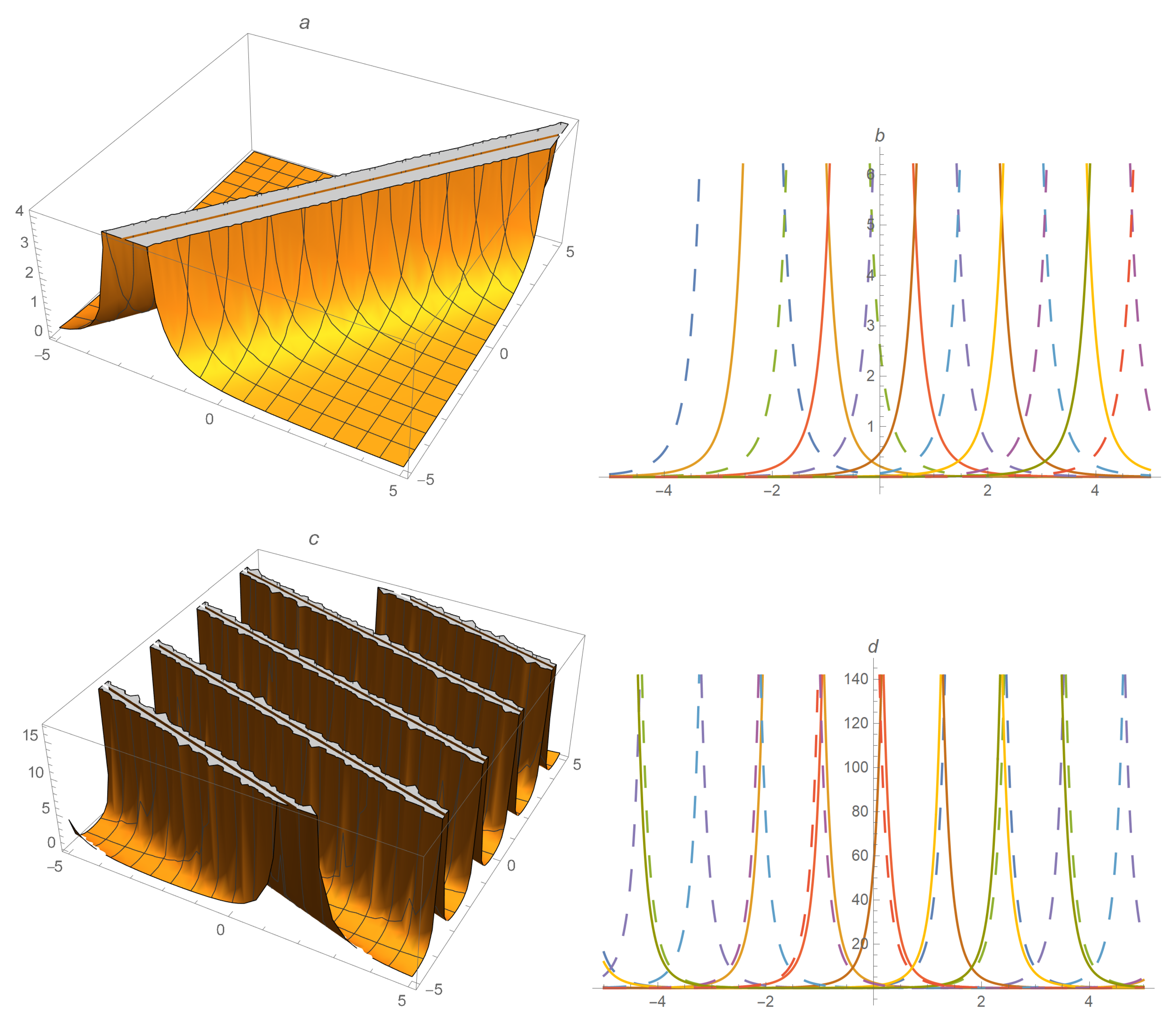
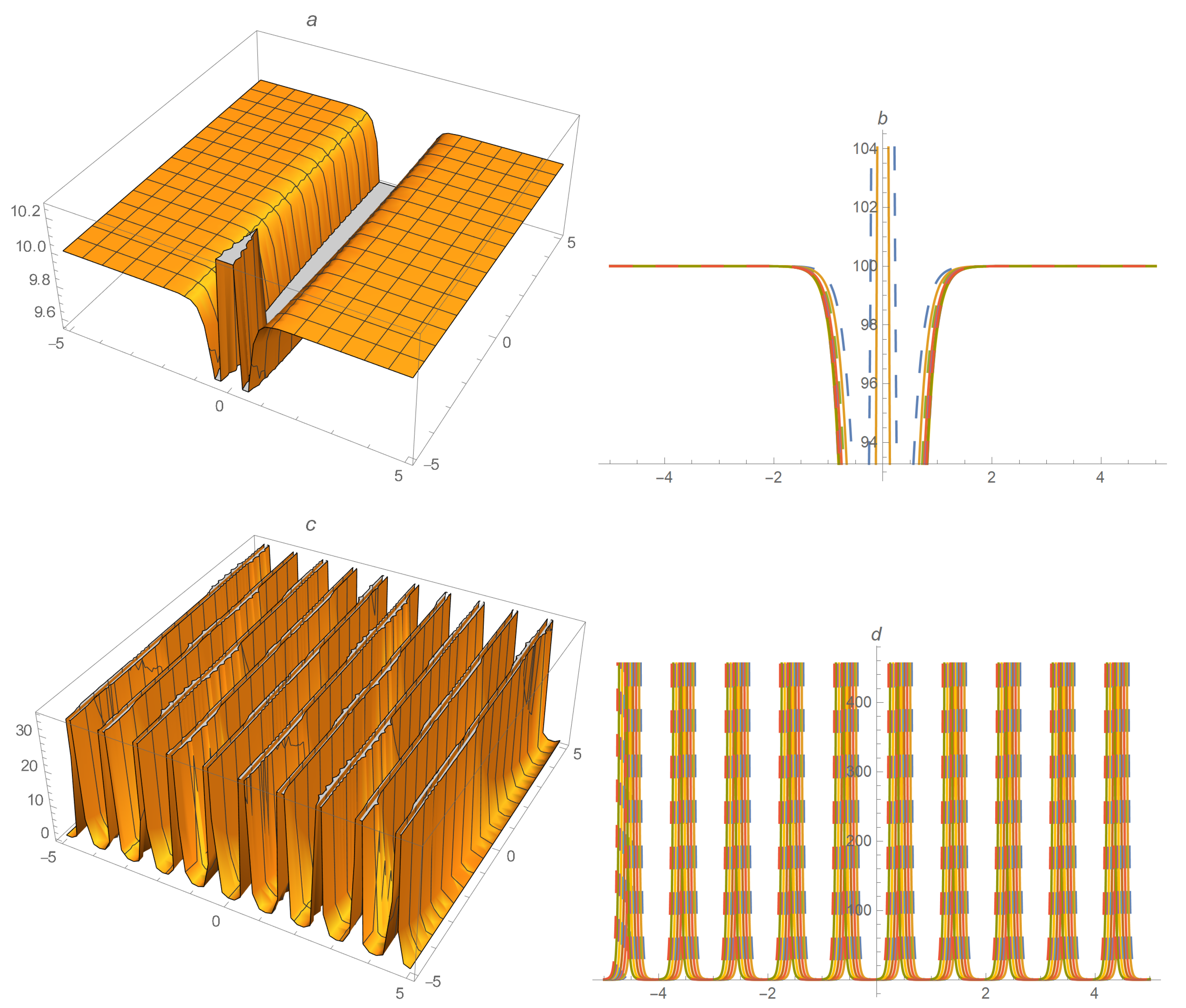
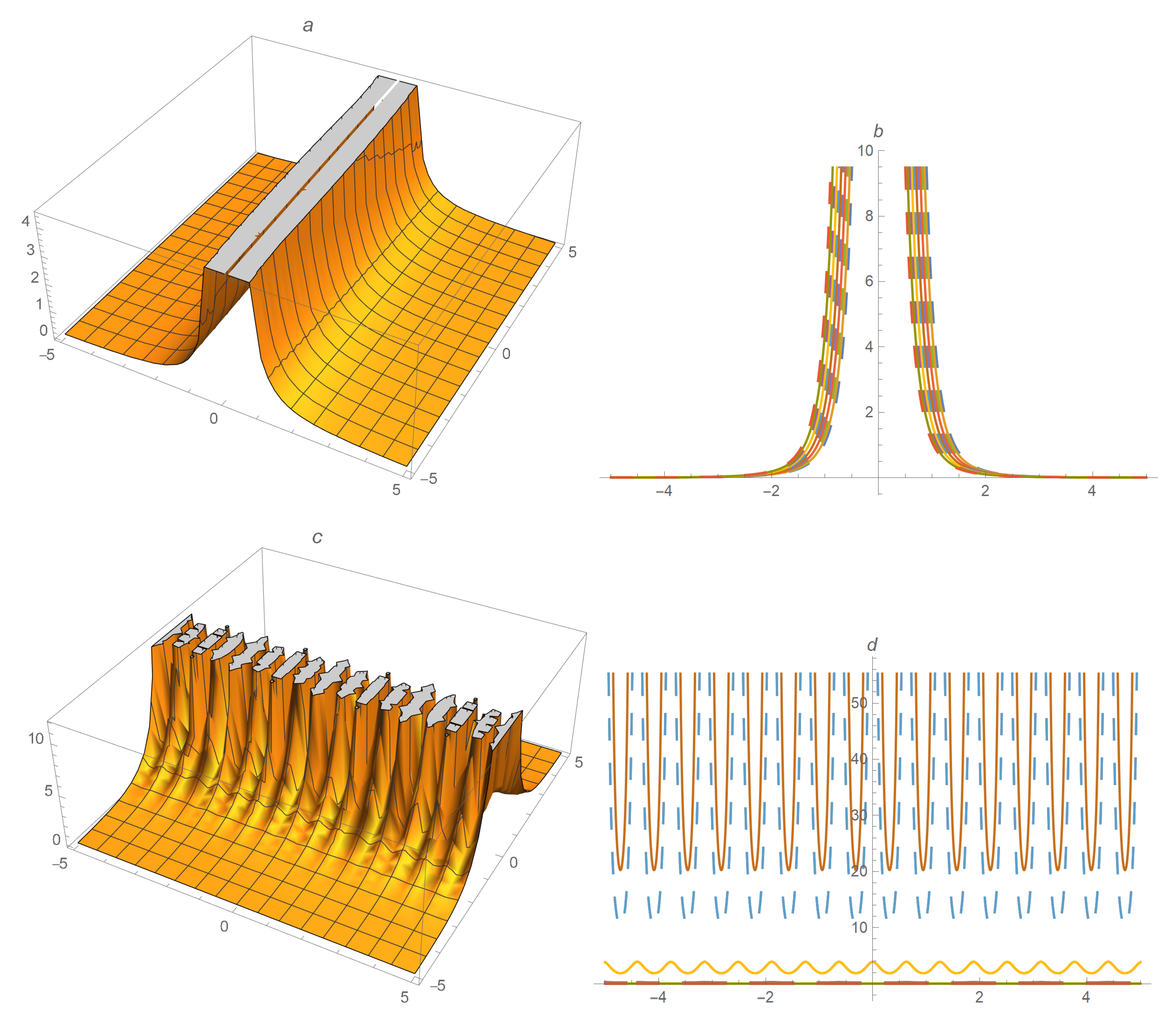
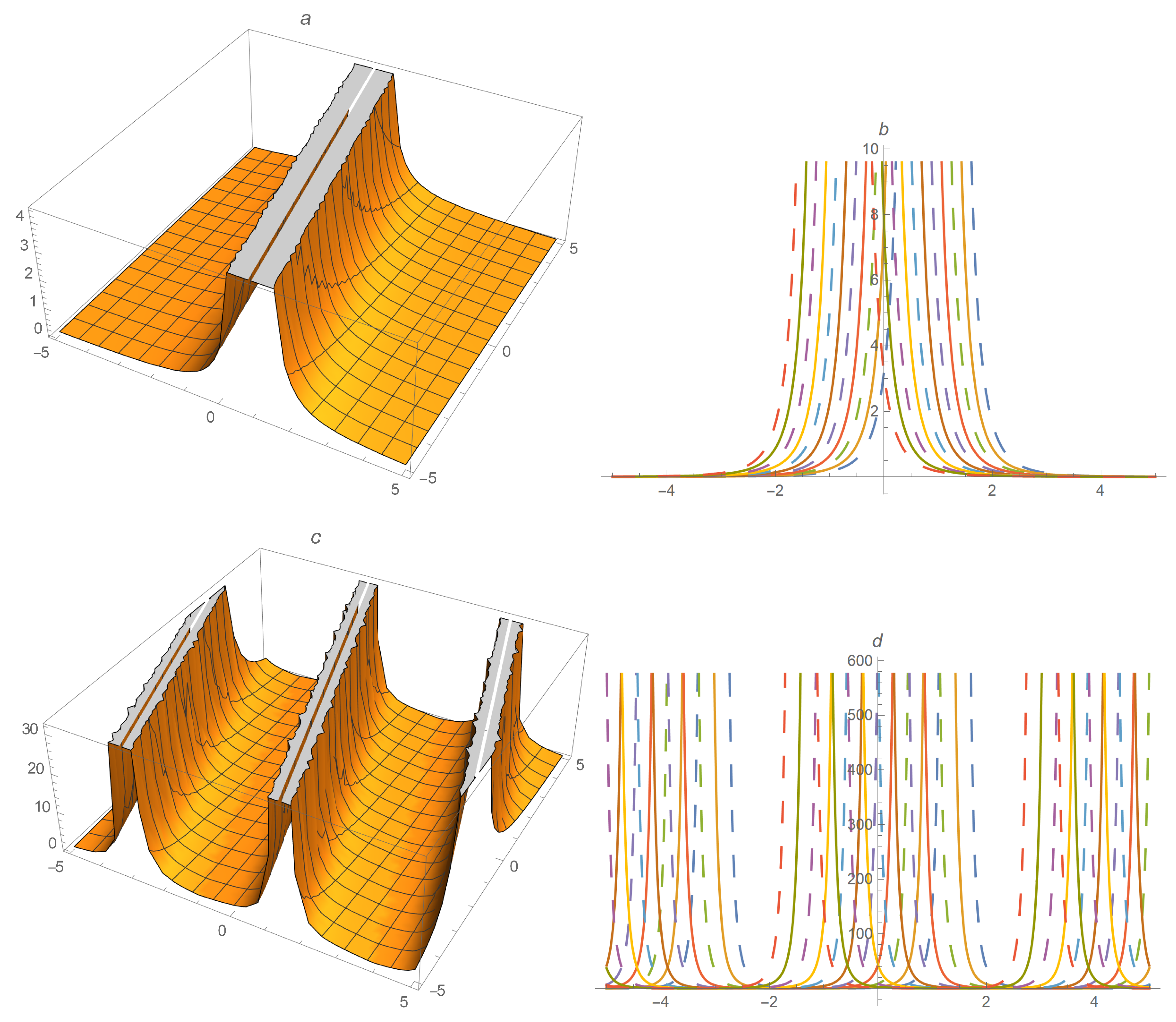
5. Results and Discussion

The mathematical methods emphasize the wave solutions of Equation (1). In the derived solutions, parameters $A_1$, $A_{-1}$, $A_2$ and $A_{-2}$ received various specific values due to these exact solutions being converted into different solitary wave solutions in different forms, such as hyperbolic, trigonometric and rational functions (Figure 1, Figure 2, Figure 3, Figure 4, Figure 5 and Figure 6). Currently several methods have been utilized to solve Equation (1) throughout the research literature [40,41,42,43,44,45,46,47,48]. Moreover, our investigated solutions are likely similar to other solutions in different research articles. Our solutions $U_6$ and $V_6$ in (35) and (36) are likely similar to the solutions $U_{41}$ in Equation (82) and $U_{42}$ in Equation (83), respectively, in [50]. Furthermore, our solutions $U_{141}$ and $V_{141}$ in (64) and (65) are similar in form to the solutions $u_2$ and $v_2$ in Equation (4.39), respectively, in [54]. Our solutions $U_8$ and $V_9$ in (41) and (42) are similar in form to the solutions $u_{23\left(\eta \right)}$ and $u_{214\left(\eta \right)}$ in Equation (50) and Equation (51), respectively, in [55]. The remainder of our derived solutions are novel and have not yet been reported in any research literature. Hence, our employed schemes are simple and useful for solving many other nonlinear problems in applied sciences.

6. Conclusions

In this study, we have proposed two novel techniques, namely, an improved form of simple equation and a modified form of F-expansion are utilized to construct exact solutions of the nonlinear fractional time space (2+1)-dimensional breaking soliton equation, via the properties of the modified Riemann-Liouville derivative. Multifarious transformation has been operated to renovate the fractional order differential equations. The constructed results have extensive potential to comprehend the interior configurations of the usual manifestations that arise in physics, mathematics and in other different fields. Hence, it is worth declaring that the execution of our techniques is extremely steady and well-organized for fractional differential equations.

References

1. Dalir, M.; Bashour, M. Application of fractional calculus. Appl. Math. Sci. 2010, 21, 1021–1032. [Google Scholar]
2. Herrmann, R. Fractional Calculus: An Introduction for Physicists; World Scientific: Singapore, 2011. [Google Scholar]
3. Javeed, S.; Saif, S.; Waheed, A.D. Baleanu, Exact solutions of the fractional mBBM equation and coupled system of fractional Boussinesq-Burgers. Respir. Physiol. 2018, 9, 1275–1281. [Google Scholar]
4. Ekici, M.; Mirzazadeh, M.; Eslami, M.; Zhou, Q.; Moshokoa, S.P.; Biswas, A. Optical soliton perturbation with fractional temporal evolution by the first integral method with conformable fractional derivatives. Opt.-Int. J. Light Elect. Opt. 2016, 127, 10659–10669. [Google Scholar] [CrossRef]
5. Younis, M. The first integral method for time-space fractional differential equations. J. Adv. Phys. 2013, 2, 220–223. [Google Scholar] [CrossRef]
6. Özkan, Y.S.; Seadawy, A.R.; Yaşar, E. Multi-wave, breather and interaction solutions to (3+1) dimensional Vakhnenko–Parkes equation arising at propagation of high-frequency waves in a relaxing medium. J. Taibah Univ. Sci. 2021, 15, 666–678. [Google Scholar] [CrossRef]
7. Younas, U.; Seadawy, A.R.; Younis, M.; Rizvi, S.T.R. Dispersive of propagation wave structures to the Dullin-Gottwald-Holm dynamical equation in a shallow water waves. Chin. J. Phys. 2020, 68, 348–364. [Google Scholar] [CrossRef]
8. Seadawy, A.R.; Iqbal, M.; Lu, D. Application of mathematical methods on the ion sound and Langmuir waves dynamical systems. Pramana J. Phys. 2019, 93, 10. [Google Scholar] [CrossRef]
9. Meng, F.; Feng, Q. Exact solution with variable coefficient function forms for conformable fractional partial differential equations by an Auxiliary equation method. Adv. Math. Phys. 2018, 2018, 4596506. [Google Scholar] [CrossRef] [Green Version]
10. Guo, S.; Zhou, Y. Auxiliary equation method for the mKdV equation with variable coefficients. Appl. Math. Comput. 2010, 217, 1476–1483. [Google Scholar] [CrossRef]
11. Zhang, S.; Zhang, H.Q. Fractional sub-equation method and its application to nonlinear fractional PDEs. Phys. Lett. 2011, 375, 1069–1073. [Google Scholar] [CrossRef]
12. Tang, B.; He, Y.; Wu, L.; Zhang, X. A generalized fractional sub-equation method for a fractional differential equation with variable coefficients. Phys. Lett. 2012, 376, 2588–2590. [Google Scholar] [CrossRef]
13. Althobaiti, A.; Althobaiti, S.; El-Rashidy, K.; Seadawy, A.R. Exact solutions for the nonlinear extended KdV equation in a stratified shear flow using modified exponential rational method. Results Phys. 2021, 29, 104723. [Google Scholar] [CrossRef]
14. Kadkhoda, N.; Jafari, H. Application of the fractional sub-equation method to the space-time fractional differential equations. Int. J. Adv. Math. Mech. 2017, 4, 1–6. [Google Scholar]
15. Zheng, B. (G/G)-expansion method for solving fractional partial differential equations in the theory of mathematical physics. Commun. Theor. Phys. 2012, 58, 623–630. [Google Scholar] [CrossRef]
16. Ahmed, I.; Seadawy, A.R.; Lu, D. M-shaped rational solitons and their interaction with kink waves in the Fokas-lenells equation. Phys. Scr. 2019, 94, 055205. [Google Scholar] [CrossRef]
17. Lu, D.; Seadawy, A.R.; Iqbal, M. Mathematical physics via construction of traveling and solitary wave solutions of three coupled system of nonlinear partial differential equations and their applications. Results Phys. 2018, 11, 1161–1171. [Google Scholar] [CrossRef]
18. Simbanefayi, I.; Khalique, C.M. Travelling wave solutions and conservation laws for the Korteweg-de Vries-Benjamin-Bona-Mahony equation. Respir. Physiol. 2018, 8, 57–63. [Google Scholar]
19. Rahmatullah, R.; Ellahi; Mohyud-Din, S.T.; Khan, U. Exact traveling wave solutions of fractional order Boussinesq-like equations by applying the Exp-function method. Respir. Physiol. 2018, 8, 114–120. [Google Scholar] [CrossRef]
20. Zheng, B. Exp-function method for solving fractional partial differential equations. Sci. World J. 2013, 2013, 465723. [Google Scholar] [CrossRef] [Green Version]
21. Ozkan, Y.G.; Yaşar, E.; Seadawy, A. On the multi-waves, interaction and Peregrine-like rational solutions of perturbed Radhakrishnan–Kundu–Lakshmanan equation. Phys. Scr. 2020, 8, 085205. [Google Scholar] [CrossRef]
22. Seadawy, A.R.; Ali, A.; Albarakati, W.A. Analytical wave solutions of the (2 + 1)-dimensional first integro-differential Kadomtsev-Petviashivili hierarchy equation by using modified mathematical methods. Results Phys. 2019, 15, 102775. [Google Scholar] [CrossRef]
23. Ray, S.S.; Sahoo, S. Two efficient reliable methods for solving fractional fifth-order modified Sawada-Kotera equation appearing in mathematical physics. J. Ocean Eng. Sci. 2016, 1, 219–225. [Google Scholar]
24. Gaber, A.A.; Aljohani, A.F.; Ebaid, A.; Machado, J.T. The generalized Kudryashov method for nonlinear space-time fractional partial differential equations of Burger’s type. Nonlinear Dynam. 2019, 95, 361–368. [Google Scholar] [CrossRef]
25. Demiray, S.T.; Bulut, H. Generalized Kudryashov method for the nonlinear fractional double Sinh-Poisson equation. J. Nonlinear Sci. Appl. 2016, 9, 1349–1355. [Google Scholar] [CrossRef] [Green Version]
26. Seadawy, A.R.; Yasmeen, A.; Raza, N.; Althobaiti, S. Novel solitary waves for fractional (2+1)-dimensional Heisenberg ferromagnetic model via new extended generalized Kudryashov method. Phys. Scr. 2021, 96, 125240. [Google Scholar] [CrossRef]
27. Kumar, D.; Seadawy, A.R.; Joardar, A.K. Modified Kudryashov method via new exact solutions for some conformable fractional differential equations arising in mathematical biology. Chin. J. Phys. 2018, 56, 75–85. [Google Scholar] [CrossRef]
28. Rahman, M.M.; Habib, M.A.; Ali, H.M.S.; Miah, M.M. The generalized Kudryashov method: A renewed mechanism for performing exact solitary wave solutions of some NLEEs. J. Mech. Cont. Math. Sci. 2019, 14, 323–339. [Google Scholar] [CrossRef]
29. Kumar, S.; Kumar, D.; Kharbanda, H. Lie symmetry analysis, abundant exact solutions and dynamics of multisolitons to the (2 + 1)-dimensional KP-BBM equation. Pramana 2021, 95, 33. [Google Scholar] [CrossRef]
30. Kumar, S.; Kumar, D.; Kumar, A. Lie symmetry analysis for obtaining the abundant exact solutions, optimal system and dynamics of solitons for a higher-dimensional Fokas equation. Chaos Solitons Fractals 2021, 142, 110507. [Google Scholar] [CrossRef]
31. Kumar, S.; Kumar, D. Lie symmetry analysis and dynamical structures of soliton solutions for the -dimensional modified CBS equation. Int. J. Mod. Phys. 2020, 34, 25. [Google Scholar] [CrossRef]
32. Kumar, S.; Kumar, A. Lie symmetry reductions and group Invariant Solutions of (2+1)-dimensional modified Veronese web equation. Nonlinear Dyn. 2019, 98, 1891–1903. [Google Scholar] [CrossRef]
33. Kumar, S.; Niwas, M.; Wazwaz, A. Lie symmetry analysis, exact analytical solutions and dynamics of solitons for (2+1)-dimensional NNV equations. Phys. Scr. 2020, 95, 095204. [Google Scholar] [CrossRef]
34. Kumar, S.; Rani, S. Lie symmetry reductions and dynamics of soliton solutions of (2+1)-dimensional Pavlov equation. Pramana 2020, 94, 116. [Google Scholar] [CrossRef]
35. Ege, S.M.; Misirli, E. Extended Kudryashov method for fractional nonlinear differential equations. Math. Sci. Appl. E-NOTE 2018, 6, 19–28. [Google Scholar] [CrossRef]
36. Akram, U.; Seadawy, A.R.; Rizvi, S.T.R.; Younis, M.; Althobaiti, S.; Sayed, S. Traveling wave solutions for the fractional Wazwaz–Benjamin–Bona–Mahony model in arising shallow water waves. Results Phys. 2021, 20, 103725. [Google Scholar] [CrossRef]
37. Gomez, C.A.; Garzon, H.G.; Hernandez, J.C.R. On exact solutions for (4þ1)-dimensional Fokas equation with variable coefficients. Adv. Stud. Theor. Phys. 2017, 11, 765–771. [Google Scholar] [CrossRef]
38. Seadawy, A.R.; Cheemaa, N. Some new families of spiky solitary waves of one-dimensional higher-order K-dV equation with power law nonlinearity in plasma physics. Indian J. Phys. 2020, 94, 117–126. [Google Scholar] [CrossRef]
39. Guner, O. Singular and non-topological soliton solutions for nonlinear fractional differential equations. Chin. Phys. B 2015, 24, 100201. [Google Scholar] [CrossRef]
40. Yildirim, Y.; Yasar, E. A (2+1)-dimensional breaking soliton equation: Solutions and conservation laws. Chaos Solit. Fractals 2018, 107, 146–155. [Google Scholar] [CrossRef]
41. Rizvi, S.T.R.; Seadawy, A.R.; Ali, I.; Bibi, I.; Younis, M. Chirp-free optical dromions for the presence of higher order spatio-temporal dispersions and absence of self-phase modulation in birefringent fibers. Mod. Phys. Lett. B 2020, 35, 2050399. [Google Scholar] [CrossRef]
42. Wazwaz, A.M. Breaking soliton equations and negative-order breaking soliton equations of typical and higher orders. Pramana Phys. 2016, 87, 68. [Google Scholar] [CrossRef]
43. Yildiz, G.; Daghan, D. Solutions of the (2+1)-dimensional breaking soliton equation by using two different methods. J. Eng. Tech. Appl. Sci. 2016, 1, 13–18. [Google Scholar]
44. Wang, S.F. Analytical multi-soliton solutions of a (2+1)-dimensional breaking soliton equation. SpringerPlus 2016, 5, 891. [Google Scholar] [CrossRef] [Green Version]
45. Chen, Y.; Ma, S. Non-traveling wave solutions for the (2+1)-dimensional breaking soliton system. Appl. Math. 2012, 3, 813–818. [Google Scholar] [CrossRef] [Green Version]
46. Zhang, J.F.; Heng, C.L. New multi-soliton solutions of the (2+1)-dimensional breaking soliton equations. Int. J. Mod. Phys. B 2003, 17, 4376–4381. [Google Scholar] [CrossRef]
47. Li, Y.S.; Zhang, Y.J. Symmetrics of a (2þ1)-dimensional breaking soliton equation: Three-wave methods. J. Phys. Math. Gen. 2012, 26, 24. [Google Scholar]
48. Darvishi, M.T.; Najafi, M. Some exact solutions of the (2+1)-dimensional breaking soliton equation using three-wave method. Int. J. Math. Comput. Sci. 2011, 5, 7. [Google Scholar]
49. Seadawy, A.R.; Ali, A.; Zahed, H.; Baleanu, D. The Klein–Fock–Gordon and Tzitzeica dynamical equations with advanced analytical wave solutions. Results Phys. 2020, 19, 103565. [Google Scholar] [CrossRef]
50. Ali, A.; Seadawy, A.R.; Baleanu, D. Computational solutions of conformable space-time derivatives dynamical wave equations: Analytical mathematical techniques. Results Phys. 2020, 19, 103419. [Google Scholar] [CrossRef]
51. Seadawy, A.; Ali, A.; Baleanu, D. Transmission of high-frequency waves in a tranquil medium with general form of the Vakhnenko dynamical equation. Phys. Scr. 2020, 95, 095208. [Google Scholar] [CrossRef]
52. Jumarie, G. Modified Riemann-Liouville derivative and fractional Taylor series of non-differentiables functions further results. Comput. Math. Appl. 2006, 51, 1367–1376. [Google Scholar] [CrossRef] [Green Version]
53. Jumarie, G. From self-similarity to the fractional derivative of non-differentiable function via Mittag-Leffler functions. Appl. Math. Sci. 2008, 2, 1949–1962. [Google Scholar]
54. Seadawy, A.R.; Cheemaa, N. Propagation of nonlinear complex waves for the coupled nonlinear Schrödinger Equations in two core optical fibers. Phys. A Stat. Mech. Appl. 2019, 529, 121330. [Google Scholar] [CrossRef]
55. Hossain, A.K.S.; Akbar, M.A.; Azad, M.A.K. The closed form solutions of simplified MCH equation and third extended fifth order nonlinear equation. Propul. Power Res. 2019, 8, 163–172. [Google Scholar] [CrossRef]
Publisher’s Note: MDPI stays neutral with regard to jurisdictional claims in published maps and institutional affiliations.