Article

Competing Risks Step-Stress Model with Lagged Effect under Gompertz Distribution

Department of Mathematics, Beijing Jiaotong University, Beijing 100044, China
*
Author to whom correspondence should be addressed.
Mathematics 2021, 9(24), 3206; https://doi.org/10.3390/math9243206
Submission received: 10 November 2021 / Revised: 8 December 2021 / Accepted: 9 December 2021 / Published: 11 December 2021
(This article belongs to the Section Probability and Statistics)

Abstract

:
In many survival analysis studies, the failure of a product may be attributed to one of several competing risks. In addition, if survival time is long, researchers can adopt accelerated life tests, causing devices to fail more quickly. One popular type of accelerated life tests is the step-stress test, and in this test, the stress level changes at a predetermined point time. The manner that stress levels change abruptly and increase discontinuously has been studied extensively. This paper considers a more realistic situation where the effect of stress increases cannot be achieved all at once, but with a lag time, and we propose a step-stress model consisting of two independent competing risks with a lag period in which the failure time caused by different risks at different stress levels obey Gompertz distribution, and the range of lag period is predetermined. The unknown parameters are estimated by maximum likelihood estimation and least squares estimation. For comparison, asymptotic confidence intervals and percentile bootstrap confidence intervals are constructed. By using Monte-Carlo simulations, we obtain the means and mean square errors of the maximum likelihood estimates and the least squares estimates, as well as the mean lengths and coverage rates of the two confidence intervals, which show the performance of various methods. Finally, in order to illustrate the model and proposed methods, we analyze a dataset from a solar energy experiment.

1. Introduction

In many survival analysis studies, the cause of failure of a product is not determined by a single risk, but by one of several competing risks. With continuous improvements in manufacturing design and technology, modern products have become more reliable and durable. In order to obtain more information regarding the lifetime of products, accelerated life tests (ALT) are taken. ALT is the process of exposing products to higher-than-normal stress conditions, causing products to fail faster than at normal stress levels. Therefore, ALT is an important means of obtaining useful information about product reliability under test time constraints. A widely used accelerated life test is the step-stress test in which the stress level begins to increase at a predetermined point. Ref. [1] considered the step-stress cumulative exposure model with time constraints when the life distributions of different risk factors are independent exponential distributions. The exact sampling distributions of maximum likelihood estimators were derived. The confidence intervals were constructed using exact distributions, asymptotic distributions, bootstrap method and Bayesian posterior distribution. Ref. [2] discussed estimation of parameters with truncated normal distribution under step-stress ALT and type-II censoring scheme. Maximum likelihood estimates were performed. The asymptotic confidence intervals were established. Bayesian estimators for three loss functions were studied. The optimal truncation schemes under different criteria were obtained. Ref. [3] presented the step-stress model with lagged effect and assumed that every test unit follows Weibull distribution. The unknown parameters were estimated by maximum likelihood method and least square method. Bayesian estimation was further discussed. Ref. [4] proposed a step-stress model for two competing risks with a linear lag period. The lifetime under each of these independent risks follows Weibull distribution. The maximum likelihood estimates asymptotic confidence intervals and percentile bootstrap confidence intervals, and the bias-corrected and accelerated percentile bootstrap confidence intervals were obtained.

1.1. Competing Risks Model

In the analysis of reliability, test units are often exposed to multiple potentially fatal risk factors and their failures are related to one of these factors. Competing risks analysis is the reliability analysis in the existence of other risk factors and has been widely studied in the fields of medicine, actuarial science and biostatistics. In a competing risks model, the observations of a test unit are often in a binary format, that is, the lifetime and the cause of the failure. The multiple causes of test unit failure can be independent or dependent. Ref. [5] studied the competing risks model of progressive hybrid censoring scheme under Gompertz distribution. They derived the maximum likelihood estimates of the parameters and obtained the confidence intervals of the model using the asymptotic approximation theory and Bootstrap method. As mentioned in Refs. [6,7], without any knowledge of the covariates, it is not feasible to test the hypothesis about whether the risks are independent. Competing risk models with independent competing risks have been extensively studied. Ref. [8] studied Bayesian analysis under Weibull distribution of progressively censored independent competing risks data. When the common shape parameters are already known, Bayesian estimators of scale parameters have closed formal expressions. When the common shape parameters are unknown, MCMC samples are used to compute Bayesian estimates and maximum posterior density confidence intervals. Ref. [9] considered step-stress ALT under type-I truncation when different risk factors obey independent generalized exponential distributions. Under the cumulative exposure model, point estimates of different parameters were derived by the maximum likelihood method. By using asymptotic distribution and parameter bootstrap method, the construction of parameter confidence intervals was discussed. For other articles in this area, see Refs. [10,11,12], etc.

1.2. Step-Stress Accelerated Life Tests

Three main stress-increasing schemes are used for ALT: constant stress, progressive stress, and step-stress. Constant stress accelerated life test means that every test unit is exposed to a constant selected stress level until the test cell fails or the test is completed. Progressive stress accelerated life test allows stress levels to increase consistently. The step-stress accelerated life test is intermediate between constant stress ALT and progressive stress ALT. Since it allows stress levels to increase at some scheduled point time, this ensures that the step-stress accelerated life test is flexible and adjustable. Step-stress ALT are widely concerned in reliability analysis. A key assumption in accelerated life tests is the cumulative exposure model (CEM). The cumulative exposure model was first proposed in Ref. [13]. The cumulative exposure model essentially provides the cumulative distribution function of lifetime. The cumulative risk model links the distribution of one stress level to the distribution of the next level, regardless of how the failure accumulated. By now, CEM has been studied extensively. Ref. [14] proposed a multi-step-stress ALT programming method with independent competition risks under a cumulative exposure model. Ref. [15] used Bayesian method to optimize step-stress accelerated life tests. Other works on CEM include Refs. [16,17,18], etc.
The hazard function of lifetime at the stress change point is discontinuous under cumulative exposure model, which means that the impact of changes in stress levels is instantaneous. Thus, a cumulative exposure model may not be reasonable in real life. Ref. [19] proposed a new step-stress model, cumulative risk model (CRM), to improve the cumulative exposure model by establishing a continuous hazard function. The cumulative risk model assumes that there is a lag period before stress changes completely. Moreover, the authors also indicated that as the lagged period is small and proceeds to zero, CEM can be obtained as a limit case of CRM where lifetime distribution follows the exponential distribution. Now, the more realistic CRM is more concerned. Ref. [20] considered statistical inferences of cumulative risk model under competing risks when the lifetime of each test unit under different risks follows exponential distribution.

1.3. Gompertz Distribution

Although the exponential distributions have many attractive features, assuming a constant hazard function may not always be more realistic in practice. Despite the fact that the Weibull distribution with two parameters is widely used in the survival and reliability literature and provides great flexibility in modeling the hazard function for step-stress tests, the hazard function is not guaranteed to be constantly increasing and may not always be reliable in step-stress accelerated tests. The Gompertz distribution model is a common model used in reliability and life testing and has two parameters, similarly to Weibull distribution. Furthermore, the Gompertz distribution can degenerate to an exponential distribution; thus, it has the superior properties of exponential distribution. Moreover, its hazard function is an increasing function, which is consistent with the conditions of stress increase in step-stress accelerated tests.
Gompertz distribution is a popular one of the popular distributions to model lifetime data with shape parameter and scale parameter. As Ref. [21] noted, Gompertz distribution was first proposed in 1825. It is widely used in financial data, bioanalytical experiments, actuarial problems, graduating age-specific mortality rates, and preparing life tables. Ref. [22] provided a theoretical justification that allows it to be employed in cases of accretionary growth. They also summarized the features and the application of Gompertz distribution. Ref. [23] proposed a Gompertz curve-fitting process, and its benefits include, without knowing the value for forecasting, the stability of the sensitivity of saturation over the sample period. Ref. [24] established an accurate confidence interval and an accurate joint confidence region for the parameters of the Gompertz distribution. Ref. [25] discussed the lifetime problem under the step-stress ALT of two independent risks with Gompertz life distribution. In Ref. [26], the failure time of a product was analyzed by using a constant stress ALT with two independent competitive risks under Gompertz distribution.
The probability density function (PDF) (see Figure 1) of Gompertz distribution with shape parameter β and scale parameter λ is as follows.
f x ; β , λ = β × exp λ x β λ × exp λ x 1 , x > 0 .
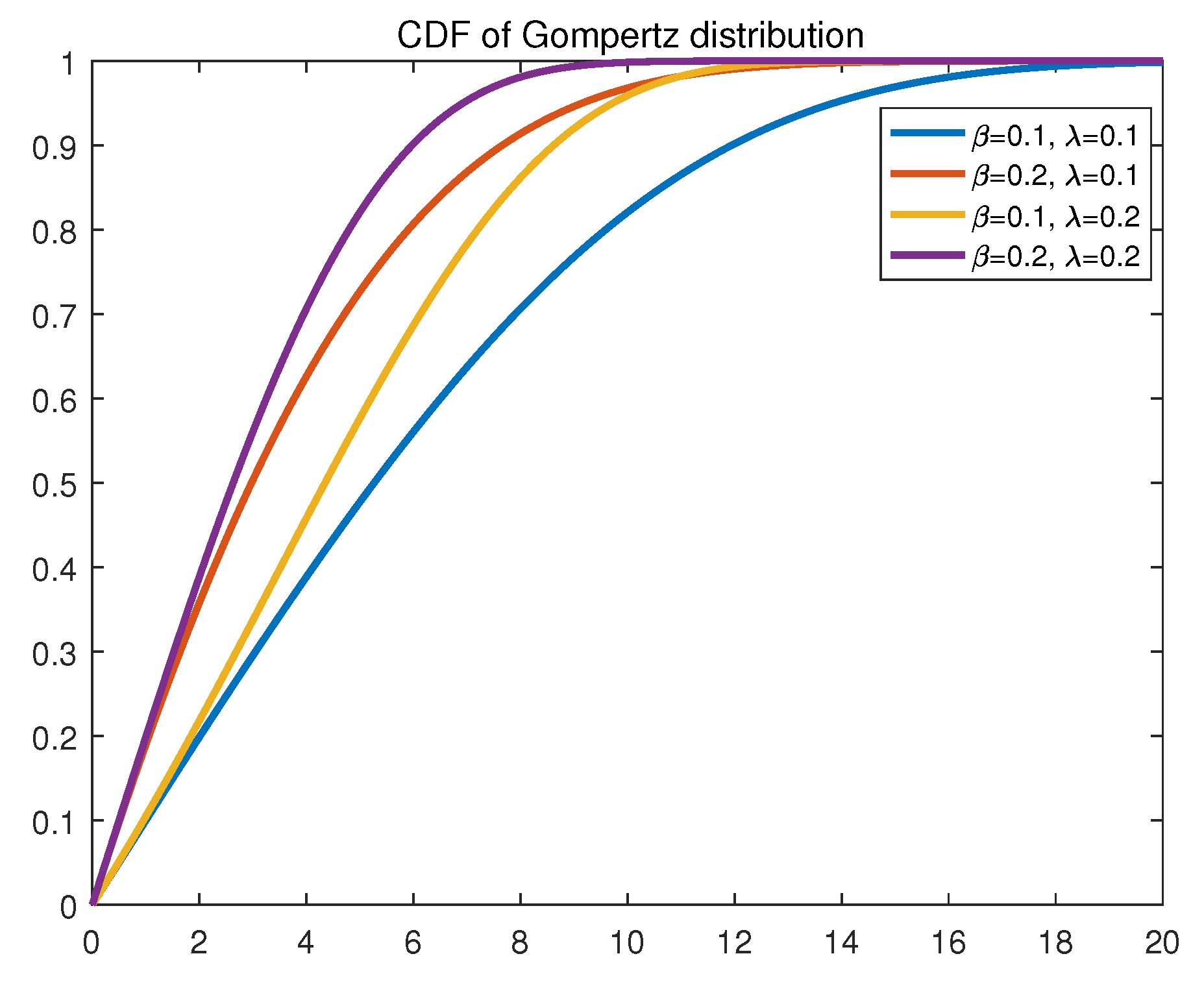
The cumulative distribution function (CDF) (see Figure 2) is obtained from the following expression.
F x ; β , λ = 1 exp β λ × exp λ x 1 , x > 0 .
The corresponding hazard function is shown below.
h x ; β , λ   =   β × exp λ x , x > 0 .
The hazard function of Gompertz distribution is increasing. When λ tends to 0, the Gompertz distribution degenerates to the exponential distribution with mean 1 β .
Continuous hazard functions reflect the impact of changes in stress levels more realistically; thus, CRM has many applications in survival analysis and solves the major limitation of existing models. The Gompertz distribution has a natural advantage in CRM modeling due to its own nature. In this paper, the Gompertz distribution is first used in CRM modeling, which provides a new method of exploring the step-stress model and addresses the main limitations of existing models.
In this paper, we study the point estimations and interval estimations of a class of step-stress models with competing risks and lagged effect based on Gompertz distribution when different competing risks are independent of each other. We make inferences using Gompertz distributions with different scale parameters and different shape parameters. The organization of the rest of the article is as follows. In Section 2, the cumulative risk model of step-stress ALT with two independent risks is described. The risk function, cumulative risk function, cumulative distribution function, and probability density function under different risk factors are deducted. In Section 3, the maximum likelihood estimates of parameters are evaluated by the Newton–Raphson method. In Section 4, the least square method is used to obtain the estimates of the parameters. In Section 5, the observed Fisher information matrix is presented. Asymptotic intervals are constructed. In Section 6, we use the percentile bootstrap method to construct confidence intervals. In Section 7, by a large number of Monte-Carlo simulations, we compare and assess the performance of estimations and confidence intervals. In Section 8, a real dataset was analyzed to illustrate the effectiveness of estimation methods. Section 9 summarizes the entire article and discusses future work in this area.

2. Model Description

Investigating step-stress ALT with n test units, all of the units come from homogeneous groups. In the initial period, all units are affected by stress level s 1 . At a predetermined time τ 1 , the stress level begins to increase. The improvement in stress level is fully realized at τ 2 and the stress level proceeds up to s 2 . δ = τ 2 τ 1 is known as the lag period. When δ = τ 2 τ 1 0 , which means τ 1 = τ 2 , CRM converges to the CEM, and the proof can be found in Appendix A.
In real situations, the lifetime of every experimental unit is often affected by several factors. This paper considers that the lifetime of every unit is affected by two risks. The failure time is denoted as X i = min X i 1 , X i 2 , i = 1 , 2 , , n , where X i j is the failure time of i-th item for the the j-th cause.
The data are recorded as ( X i , C i , I i ) : i = 1 , 2 , , n , where X i = t i > 0 represents failure time, C i = 1 ( 2 ) represents failure cause and I i represents the stress level of the i-th unit,
I i = 1 0 < t i < τ 1 , 2 τ 1 t i < τ 2 , 3 τ 2 t i .
We denote ( 0 , τ 1 ) , [ τ 1 , τ 2 ) and [ τ 2 , + ) as interval 1, interval 2 and interval 3, respectively. n j k is the total number of units that fail resulting from the j-th risk within time interval k ( k = 1 , 2 , 3 ) . n k is the total number of units that fail within time interval k ( k = 1 , 2 , 3 ) . n j is the total number of units that fail resulting from the j-th risk in the entire time range. Considering lagged effect and two potential risks of failure, there is n 1 + n 2 = n 1 + n 2 + n 3 = n , where n is the number of all units observed in the test. Ref. [25] argued that shape parameters are related to risk factors and scale parameters are related to stress levels. All shape parameters and scale parameters are greater than zero. A similar assumption is used in this article. β 1 and β 2 are associated with risk factors. λ 1 and λ 2 are associated with stress levels.
We assume that the hazard functions in the cumulative risk model of step-stress ALT increase linearly during the lag period, and Ref. [4] made the same assumption. By using the CRM of step-stress ALT, we obtained the hazard function h j ( t ) under the Gompertz distribution of the j-th risk factor for j = 1 , 2 .
h j ( t ) = β j × e λ 1 t 0 < t < τ 1 , a j + b j t τ 1 t < τ 2 , β j × e λ 2 t τ 2 t .
In order to obtain a continuous hazard function over the life span, a j and b j should satisfy the following conditions.
β j × e λ 1 τ 1 = a j + b j τ 1 β j × e λ 1 τ 2 = a j + b j τ 2
The cumulative hazard function H j ( t ) for the j-th failure cause under CRM of step-stress ALT with two risks is as follows.
H j ( t ) = β j τ 1 ln ( a j + b j τ 1 ) ln β j a j + b j τ 1 β j t τ 1 1 0 < t < τ 1 , a j + b j τ 1 β j τ 1 ln ( a j + b j τ 1 ) ln β j + a j t τ 1 + b j 2 t 2 τ 1 2 τ 1 t < τ 2 , a j + b j τ 1 β j τ 1 ln ( a j + b j τ 1 ) ln β j + a j τ 2 τ 1 + b j 2 τ 2 2 τ 1 2 + β j τ 2 ln ( a j + b j τ 2 ) ln β j a j + b j τ 2 β j t τ 2 a j + b j τ 2 β j τ 2 t .
The cumulative distribution function (CDF) G j ( t ) of the lifetime for the j-th failure cause is as follows.
G j ( t ) = 1 exp β j τ 1 ln ( a j + b j τ 1 ) ln β j a j + b j τ 1 β j t τ 1 1 , 0 < t < τ 1 , 1 exp a j + b j τ 1 β j τ 1 ln ( a j + b j τ 1 ) ln β j a j t τ 1 b j 2 t 2 τ 1 2 τ 1 t < τ 2 , 1 exp a j + b j τ 1 β j τ 1 ln ( a j + b j τ 1 ) ln β j a j τ 2 τ 1 b j 2 τ 2 2 τ 1 2 × exp β j τ 2 ln ( a j + b j τ 2 ) ln β j a j + b j τ 2 β j t τ 2 a j + b j τ 2 β j τ 2 t .
The probability density function (PDF) g j ( t ) of the lifetime for the j-th failure cause is as follows.
g j ( t ) = β j a j + b j τ 1 β j t τ 1 exp β j τ 1 ln ( a j + b j τ 1 ) ln β j a j + b j τ 1 β j t τ 1 1 0 < t < τ 1 , a j + b j t exp a j + b j τ 1 β j τ 1 ln ( a j + b j τ 1 ) ln β j a j t τ 1 b j 2 t 2 τ 1 2 τ 1 t < τ 2 , β j a j + b j τ 2 β j t τ 2 exp a j + b j τ 1 β j τ 1 ln ( a j + b j τ 1 ) ln β j a j τ 2 τ 1 b j 2 τ 2 2 τ 1 2 × exp β j τ 2 ln ( a j + b j τ 2 ) ln β j a j + b j τ 2 β j t τ 2 a j + b j τ 2 β j τ 2 t .
Considering two independent competing factors, the cumulative distribution function F X ( t ) of lifetime is shown below.
F X ( t ) = 1 1 G 1 ( t ) 1 G 2 ( t ) = 1 exp H 1 ( t ) + H 2 ( t ) .
The PDF of lifetime f X ( t ) is described by the following expression.
f X ( t ) = d F X ( t ) d t = h 1 ( t ) + h 2 ( t ) exp H 1 ( t ) + H 2 ( t ) .
The joint probability density function f X , C ( t , j ) of lifetime and failure cause, with two independent competing risks, is as shown below.
f X , C ( t , j ) = g j ( t ) ( 1 G 3 j ( t ) ) .
The explicit expressions of F X ( t ) , f X ( t ) and f X , C ( t , j ) are provided in Appendix B.

3. Maximum Likelihood Estimation

Maximum likelihood estimation (MLE) is one of the most extensively used methods for parameter estimation. In this section, we reparameterize the parameters according to the continuity of the hazard functions, apply the new parameters to the maximum likelihood function and obtain point estimates of the new parameters.
By (11), the likelihood function L is as follows:
L ( ( a 1 , a 2 , b 1 , b 2 , β 1 , β 2 ) | | ( t i , c i ) ) = i = 1 n f ( t i , c i ) = i = 1 n j = 1 2 f ( t i , c i ) I ( c i = j ) = I i = 1 j = 1 2 f ( t i , c i ) I ( c i = j ) I i = 2 j = 1 2 f ( t i , c i ) I ( c i = j ) I i = 3 j = 1 2 f ( t i , c i ) I ( c i = j ) ,
where I ( c i = j ) is an indicator function.
The corresponding log-likelihood function l is the following.
l = ln L ( a 1 , a 2 , b 1 , b 2 , β 1 , β 2 | | ( t i , c i ) ) = n 1 ln β 1 + n 2 ln β 2 n 2 ln ( τ 2 τ 1 ) ( n 2 + n 3 ) ( β 1 + β 2 ) τ 1 ln ( a j + b j τ 1 β j ) a j + b j τ 1 β j 1 + 1 τ 1 ln a j + b j τ 1 β j I i = 1 t i + I i = 2 ln ( τ 2 t i ) a j + b j τ 1 β j + ( t i τ 1 ) a j + b j τ 2 β j + 1 τ 2 ln a j + b j τ 2 β j I i = 3 t i ( β 1 + β 2 ) I i = 3 τ 2 ln ( a j + b j τ 2 β j ) a j + b j τ 2 β j t i τ 2 a j + b j τ 2 β j ( β 1 + β 2 ) I i = 2 a j ( t i τ 1 ) β j + b j ( t i 2 τ 1 2 ) 2 β j ( β 1 + β 2 ) I i = 1 τ 1 ln ( a j + b j τ 1 β j ) a j + b j τ 1 β j t i τ 1 1 ( β 1 + β 2 ) n 3 a j β j ( τ 2 τ 1 ) + b j 2 β j ( τ 2 2 τ 1 2 ) .

Reparameterization

Continuity conditions in (5) are used to reparameterize original model terms. New parameters are applied to the maximum likelihood function. This form renders the function simpler when performing subsequent calculations and simulations.
Express the function l using β 1 , β 2 , λ 1 and λ 2 .
l = n 1 ln β 1 + n 2 ln β 2 + λ 1 I i = 1 t i + I i = 2 ln ( τ 2 e λ 1 τ 1 τ 1 e λ 2 τ 2 ) + ( e λ 2 τ 2 e λ 1 τ 1 ) t i + λ 2 I i = 3 t i n 2 ln ( τ 2 τ 1 ) ( β 1 + β 2 ) I i = 1 e λ 1 t i 1 λ 1 ( β 1 + β 2 ) I i = 2 e λ 1 τ 1 1 λ 1 + τ 2 e λ 1 τ 1 τ 1 e λ 2 τ 2 τ 2 τ 1 ( t i τ 1 ) + e λ 2 τ 2 e λ 1 τ 1 τ 2 τ 1 t i 2 τ 1 2 2 ( β 1 + β 2 ) I i = 3 e λ 1 τ 1 1 λ 1 + τ 2 e λ 1 τ 1 τ 1 e λ 2 τ 2 + ( e λ 2 τ 2 e λ 1 τ 1 ) τ 1 + τ 2 2 + e λ 2 t i e λ 2 τ 2 λ 2 .
In order to obtain estimates of β 1 , β 2 , λ 1 and λ 2 , the partial derivatives of log-likelihood function for β 1 , β 2 , λ 1 and λ 2 are set to 0. Based on that, we have the following four equations. The concrete equations are provided in Appendix C.
l β 1 = 0 , l β 2 = 0 , l λ 1 = 0 , l λ 2 = 0 .
By solving these equations, we can obtain the maximum likelihood estimates β ^ 1 , β ^ 2 , λ ^ 1 and λ ^ 2 of four parameters. The log-likelihood function can be maximized when the estimates are used as parameters. However, these equations are highly nonlinear, and it is not feasible to obtain analytical solutions. In order to solve this problem, numerical techniques are indispensable. The Newton–Raphson method is used to obtain maximum likelihood estimates of β ^ 1 , β ^ 2 , λ ^ 1 and λ ^ 2 , and the Newton–Raphson method can be implemented by R software.

4. Least Squares Estimation

In this section, we provide least squares estimation (LSE) to estimate β 1 and β 2 when λ 1 and λ 2 are known. Since a 1 , a 2 , b 1 and b 2 can be expressed in terms of β 1 , β 2 , λ 1 and λ 2 , estimates of a 1 , a 2 , b 1 and b 2 can also be obtained by using this method.
From Equation (5), a j and b j can be expressed as follows.
a j = β j × τ 2 e λ 1 τ 1 τ 1 e λ 2 τ 2 τ 2 τ 1 , b j = β j × e λ 2 τ 2 e λ 1 τ 1 τ 2 τ 1 .
The cumulative hazard function H ( t ) of lifetime under the two competing risks is shown below:
H ( t ) = ln ( S ( t ) ) = ln ( 1 G 1 ( t ) ) ( 1 G 2 ( t ) ) = ln ( 1 G 1 ( t ) ) ln ( 1 G 2 ( t ) ) = H 1 ( t ) + H 2 ( t ) = D ( t ) ( β 1 + β 2 ) ,
where S ( t ) is the cumulative survival function of lifetime under two independent competing risks, S ( t ) = 1 F X ( t ) , and D ( t ) is denoted as follows.
D ( t ) = e λ 1 t 1 λ 1 0 < t < τ 1 , e λ 1 τ 1 1 λ 1 + τ 2 e λ 1 τ 1 τ 1 e λ 2 τ 2 τ 2 τ 1 ( t τ 1 ) + e λ 2 τ 2 e λ 1 τ 1 τ 2 τ 1 t 2 τ 1 2 2 τ 1 t < τ 2 , e λ 1 τ 1 1 λ 1 + τ 2 e λ 1 τ 1 τ 1 e λ 2 τ 2 + ( e λ 2 τ 2 e λ 1 τ 1 ) τ 1 + τ 2 2 + e λ 2 t e λ 2 τ 2 λ 2 τ 2 t .
The empirical cumulative risk function H ˜ ( t i ) can be derived from the empirical survival function S ˜ ( t i ) .
H ˜ ( t i ) = ln S ˜ ( t i ) = ln n i + 0.01 n , i = 1 , 2 , , n .
We note that, under CRM, the cumulative risk function is linear for β 1 and β 2 when λ 1 and λ 2 are fixed. Therefore, the estimates of β 1 and β 2 can be obtained by minimizing H ( t i ) and H ˜ ( t i ) .
The squares distance function f ( β 1 , β 2 | | λ 1 , λ 2 ) is as follows.
f ( β 1 , β 2 | | λ 1 , λ 2 ) = i = 1 n H ( t i ) H ˜ ( t i ) 2 .
From Equations (17) and (19), the expression of function (20) is as follows.
f ( β 1 , β 2 | | λ 1 , λ 2 ) = I i = 1 H ( t i ) H ˜ ( t i ) 2 + I i = 2 H ( t i ) H ˜ ( t i ) 2 + I i = 3 H ( t i ) H ˜ ( t i ) 2 = i = 1 n D ( t i ) β 1 + β 2 H ˜ ( t i ) 2 .
In order to obtain estimates β 1 ˜ and β 2 ˜ , the derivatives of the squares distance function for β 1 and β 2 are set to zero. By solving these equations, the least squares estimates β 1 ˜ and β 2 ˜ are obtained. The squares distance function is minimized when the estimates are used as parameters.
β 1 ˜ + β 2 ˜ = i = 1 n D ( t i ) H ˜ ( t i ) i = 1 n D ( t i ) 2 .
In order to obtain the respective estimates of β 1 and β 2 , we note that the relationship between β 1 and β 2 as follows:
P ( c = 1 ) = 0 + f X , C ( t , 1 ) d t = 0 + g 1 ( t ) ( 1 G 2 ( t ) ) d t = 0 + h 1 ( t ) e ( H 1 ( t ) + H 2 ( t ) ) d t = 0 + β 1 D ( t ) e D ( t ) ( β 1 + β 2 ) = β 1 β 1 + β 2 ,
where P ( c = 1 ) indicates the probability that failure is due to risk factor 1. D ( t ) indicates the derivative of D ( t ) .
n 1 n P ( c = 1 ) = β 1 β 1 + β 2 .
Apply (24) to function (22), the least squares estimates of β 1 , β 2 , a j and b j for given λ 1 and λ 2 can be obtained as follows.
β 1 ˜ = n 1 n i = 1 n D ( t i ) H ˜ ( t i ) i = 1 n D ( t i ) 2 , β 2 ˜ = n 2 n i = 1 n D ( t i ) H ˜ ( t i ) i = 1 n D ( t i ) 2 , a j ˜ = β j ˜ × τ 2 e λ 1 τ 1 τ 1 e λ 2 τ 2 τ 2 τ 1 , b j ˜ = β j ˜ × e λ 2 τ 2 e λ 1 τ 1 τ 2 τ 1 .
If λ 1 and λ 2 are known in advance, LSE is directly used to obtain the estimates of a 1 , a 2 , b 1 , b 2 , β 1 and β 2 . If λ 1 and λ 2 are not known quantities, the estimates of λ 1 and λ 2 can be derived by MLE, and the obtained estimates are used as the true values of λ 1 and λ 2 . Afterwards, we use LSE to obtain the estimates of a 1 , a 2 , b 1 , b 2 , β 1 and β 2 .

5. Asymptotic Confidence Intervals

As the sample size increases, maximum likelihood estimators have asymptotic normality and the distributions of the estimators approach normal distributions. The means of the normal distributions are the true values of the parameters. The variance–covariance matrix is acquired by inverting Fisher information matrix. Moreover, as the sample size becomes large, the biases of the estimators tend to 0, and the variances reach Cramer–Rao lower bounds. Maximum likelihood estimators are asymptotically unbiased and efficient. In this part, using these properties of maximum likelihood estimation, we obtain the asymptotic intervals of β 1 , β 2 , λ 1 and λ 2 .

Observed Fisher Information Matrix

For constructing the asymptotic intervals of β 1 , β 2 , λ 1 and λ 2 , the asymptotic variance–covariance matrix of the four parameters is discussed by the inversion of the observed Fisher information matrix.
Fisher information matrix I ( β 1 , β 2 , λ 1 , λ 2 ) can be calculated by taking the expectation of the negative second derivative of the log-likelihood function.
I ( β 1 , β 2 , λ 1 , λ 2 ) = E 2 l β 1 2 2 l β 1 β 2 2 l β 1 λ 1 2 l β 1 λ 2 2 l β 2 β 1 2 l β 2 2 2 l β 2 λ 1 2 l β 2 λ 2 2 l λ 1 β 1 2 l λ 1 β 2 2 l λ 1 2 2 l λ 1 λ 2 2 l λ 2 β 1 2 l λ 2 β 2 2 l λ 2 λ 1 2 l λ 2 2 .
It is not feasible to obtain Fisher information matrix I by calculating the expectation of the second derivative. By substituting β 1 ^ , β 2 ^ , λ 1 ^ and λ 2 ^ for β 1 , β 2 , λ 1 and λ 2 , the elements of the observed Fisher information matrix I o can be used to approximate the elements in (26). The elements of the observed Fisher information matrix are presented in Appendix D.
I o = I ( β 1 ^ , β 2 ^ , λ 1 ^ , λ 2 ^ ) = A 11 A 12 A 13 A 14 A 21 A 22 A 23 A 24 A 31 A 32 A 33 A 34 A 41 A 42 A 43 A 44 .
By inverting the matrix in (27), the variance–covariance matrix of β 1 ^ , β 2 ^ , λ ^ 1 and λ ^ 2 is obtained.
C o v ( β 1 ^ , β 2 ^ , λ 1 ^ , λ 2 ^ ) = σ 11 σ 12 σ 13 σ 14 σ 21 σ 22 σ 23 σ 24 σ 31 σ 32 σ 33 σ 34 σ 41 σ 42 σ 43 σ 44 = I ( β 1 ^ , β 2 ^ , λ 1 ^ , λ 2 ^ ) 1 .
Let V = ( σ 11 , σ 22 , σ 33 , σ 44 ) , θ = ( β 1 , β 2 , λ 1 , λ 2 ) , and θ ^ = ( β 1 ^ , β 2 ^ , λ 1 ^ , λ 2 ^ ) .
Under the regularity condition, θ ^ is asymptotically unbiased for θ , and θ ^ θ V asymptotically follow the standard normal distributions. Thus, θ ^ θ V is used as a pivotal quantity for θ . Since the parameters to be estimated are non-negative, the lower bounds of the confidence intervals must be greater than zero.
The two-sided 100 ( 1 α ) % asymptotic confidence interval (ACI) is described as follows:
max 0 , θ ^ U α / 2 V , θ ^ + U α / 2 V ,
where U α / 2 is the upper α 2 -th quantile of the standard normal distribution.

6. Percentile Bootstrap Confidence Intervals

Bootstrap method is an effective tool for constructing confidence intervals via resampling, and the percentile bootstrap (Boot-p) method is commonly used. This section presents the construction of the percentile bootstrap confidence intervals utilizing simulated data. The algorithms of simulating sample data and generating Boot-p confidence intervals are demonstrated as follows, and the expression of coverage rates is given.
Algorithm 1 provides a method to simulate failure time by considering two competing risks. For each of the two risks, failure times X i 1 and X i 2 are simulated. Since only the shortest lifetimes are observed in the analysis of competing risks, the shortest times of X i 1 and X i 2 and the associated cause of failure are recorded. The specific algorithm is shown below.
Algorithm 1: Simulating sample data.
Step 1:
Generate two independent random variables with identical uniform distribution from 0 to 1, and generate two sets produced by those two random variables, whose capacity is n.
Step 2:
Calculate the CDFs in (7) at t = τ 1 and t = τ 2 . Invert the CDFs of the two causes to generate failure time.
Step 3:
Determine the minimum time of failure generated in Step 2 for each unit and the cause of failure. Denote the failure time as ( T i , C i ) , i = 1 , 2 , n . If a certain dataset satisfies [ n 11 = 0 and ( n 12 = 0 or n 13 = 0 ) ] or [ n 21 = 0 and ( n 22 = 0 or n 23 = 0 ) ] , discard this dataset and generate a new one.
The percentile bootstrap is a resampling method. Its details are described in Ref. [27]. With Algorithm 2, the percentile bootstrap intervals (BPI) under the step-stress ALT taking into account lagged effects and two competing risks are constructed.
Algorithm 2: Generating Boot-p confidence intervals.
Step 1:
Calculate θ ^ , the MLEs of θ from the original sample, through the optimization of (14).
Step 2:
Using the estimates θ ^ as Algorithm 1, generate a new dataset of size n, denoting it as T i * , C i * , i = 1 , 2 , n .
Step 3:
Estimate MLEs θ ^ * as Step 1, based on T i * , C i * .
Step 4:
Set the amount of simulation N b o o t times beforehand. Repeat Steps 2–3 N b o o t times, obtaining a total of N b o o t θ ^ * s.
Step 5:
Sort each element of N b o o t θ ^ * s separately. Taking λ 1 ^ * as an example, the Boot-p confidence interval at 100 ( 1 α ) % coverage rate of λ 1 is expressed in the following. The Boot-p confidence intervals of other parameters are gained in the same way:
λ 1 ^ ( N b o o t × α 2 ) * , λ 1 ^ ( N b o o t × 2 α 2 ) *
In order to calculate coverage rates, set the number of repetitions N C I and run steps 1–5 for N C I times. The coverage rates of Boot-p confidence intervals are calculated by computing the proportion of true values falling into the confidence intervals. Here, we calculate the coverage rate of λ 1 as an example:
C R λ 1 = i = 1 N C I 1 λ 1 ^ ( L ) * λ 1 λ 1 ^ ( U ) * N C I ,
where I λ 1 ^ ( L ) * λ 1 λ 1 ^ ( U ) * is an indicator function, and λ 1 ^ ( L ) * = λ 1 ^ ( N b o o t × α 2 ) * , λ 1 ^ ( U ) * = λ 1 ^ ( N b o o t × 2 α 2 ) * .

7. Numerical Study

This section uses Monte-Carlo simulations to evaluate the properties of MLE and LSE and ACI and BPI. Here, the R software is used for calculations and simulations. We predetermined four sets of true values for simulation, and the true values are set as follows:
  • True Values I: τ 1 = 3, τ 2 = 6, β 1 = 0.2, β 2 = 0.1, λ 1 = 1/10, λ 2 = 1/5;
  • True Values II: τ 1 = 3, τ 2 = 6, β 1 = 0.15, β 2 = 0.1, λ 1 = 1/10, λ 2 = 1/5;
  • True Values III: τ 1 = 4, τ 2 = 6, β 1 = 0.2, β 2 = 0.1, λ 1 = 1/10, λ 2 = 1/5;
  • True Values IV: τ 1 = 4, τ 2 = 6, β 1 = 0.15, β 2 = 0.1, λ 1 = 1/10, λ 2 = 1/5.
The means and mean square errors (MSE) demonstrate the performance of MLE and LSE. Four sets of data are predetermined as true values using Algorithm 1 to generate random numbers under different true values as samples. When using maximum likelihood estimation, estimates of the unknown parameters based on the samples are obtained by using the optim command in R software. When using LSE, λ 1 and λ 2 are considered as known and are the corresponding predefined true values. Due to the randomness of the simulation, sampling is repeated n = 1000 times, and the average value is taken as the final value. We also calculated the mean square error. Table 1, Table 2, Table 3 and Table 4 report the means and mean square errors of the maximum likelihood estimates and the least square estimates for different true values.
For interval estimation, the performance of asymptotic confidence intervals and percentile bootstrap confidence intervals is demonstrated by the mean interval lengths (ML) and coverage rates (CR). For ACI, maximum likelihood estimates and the variance–covariance matrix were used to obtain asymptotic confidence intervals. The sampling is repeated n = 1000 times to calculate the mean interval lengths and the coverage rates of the asymptotic confidence intervals. For BPI, due to a large number of iterations of the Boot-p algorithm, it is time costly to perform too much repetitive sampling in practical applications. In this paper, we show the ML and CR of Boot-p confidence intervals with repeated sampling n = 100 . Table 5 and Table 6 report ML and CR of asymptotic confidence intervals and Boot-p confidence intervals at 95 % confidence level and 99 % confidence level respectively under True Value I. Table 7 and Table 8 report ML and CR of asymptotic confidence intervals and Boot-p confidence intervals at 95 % confidence level and 99 % confidence level respectively under True Value II. Table 9 and Table 10 report ML and CR of asymptotic confidence intervals and Boot-p confidence intervals at 95 % confidence level and 99 % confidence level respectively under True Value III. Table 11 and Table 12 report ML and CR of asymptotic confidence intervals and Boot-p confidence intervals at 95 % confidence level and 99 % confidence level respectively under True Value IV.
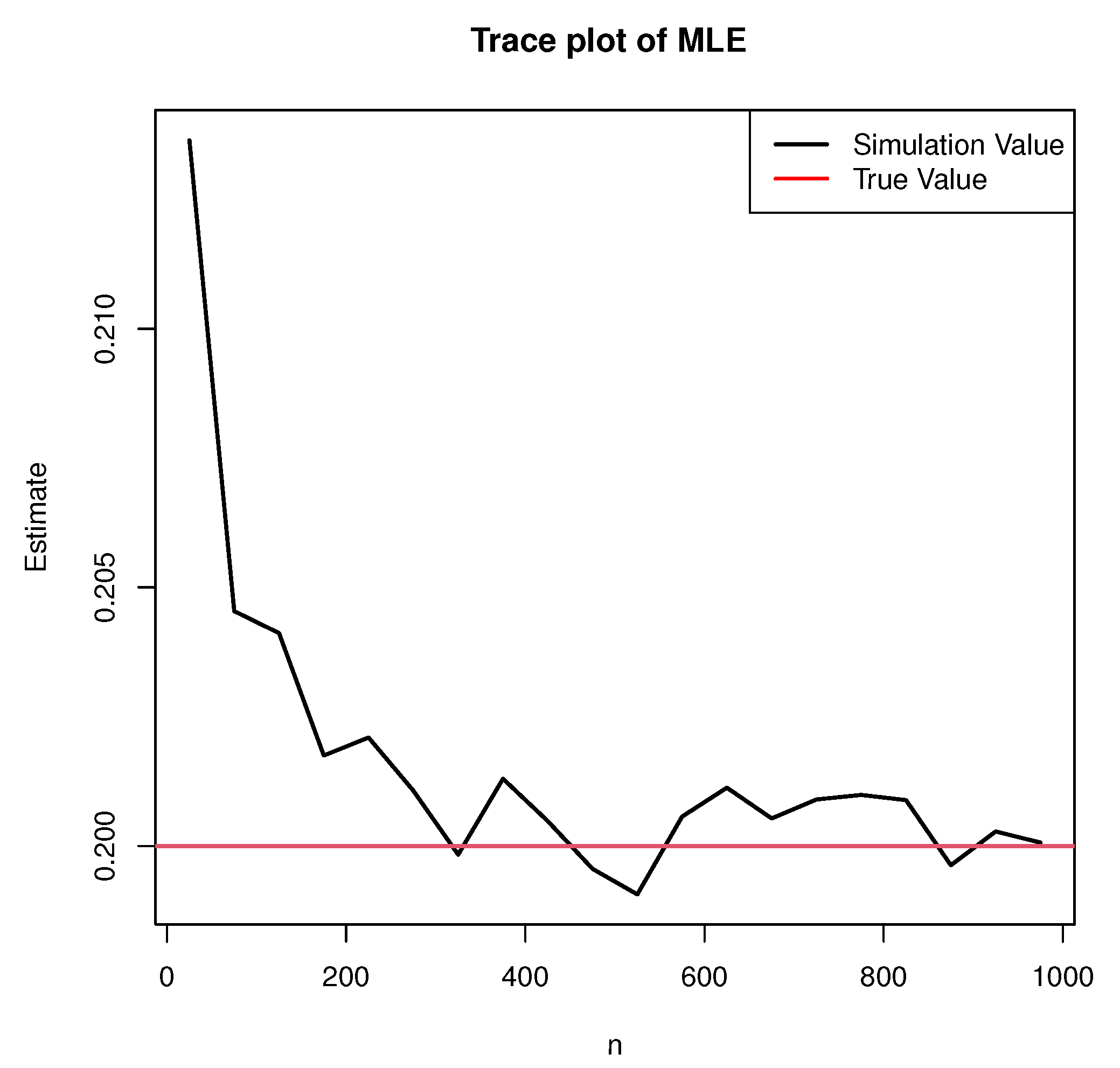
From Table 1, Table 2, Table 3 and Table 4, the following conclusions can be drawn. Taking β 1 as an example, the estimates using MLE and LSE at different sample sizes n under the True Value I are shown in Figure 3 and Figure 4.
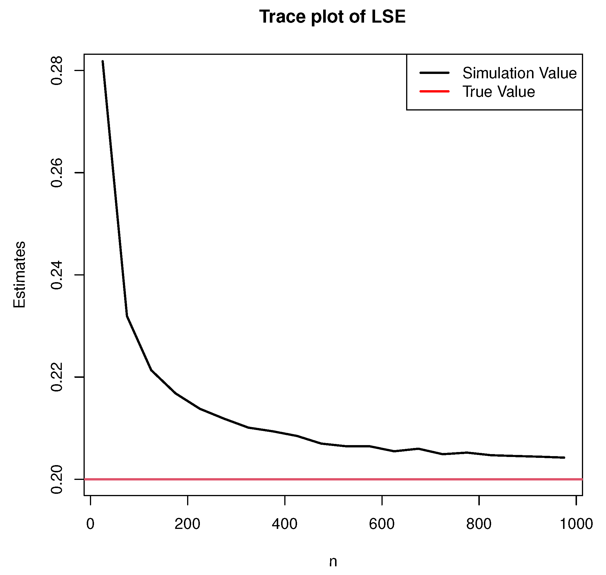
(1) With an increased sample size n, the estimates of both MLE and LSE converge to true values, and the mean square errors gradually reduce and tend to zero.
(2) From the perspective of mean value and mean square error, there is no significant difference between the mean square error of MLE and LSE. However, the maximum likelihood estimates are much closer to the true value than the least squares estimates. This is because the least square method minimizes the sum of the squares of the distances between the observed and estimated points. On the other hand, the maximum likelihood estimation is intended for maximizing the probability of drawing observations from the model. The purpose of the least square estimation method is to obtain the parameters that make the model best fit the sample data. When using LSE in the case of small samples, it produces large errors, which is consistent with simulation results.
(3) For different true values, there is no significant difference in the fitting effect. Moreover, the mean squared errors of λ ^ 1 and λ ^ 2 are significantly larger than the MSEs of β ^ 1 and β ^ 2 , which means that the simulation errors of β 1 and β 2 are smaller under the same conditions.
The following conclusions can be drawn from Table 5, Table 6, Table 7, Table 8, Table 9, Table 10, Table 11 and Table 12.
(1) With an increasing sample size n, the mean interval lengths of ACI and BPI become slimmer, and the coverage rates of asymptotic credible intervals and Boot-p credible intervals are very close to CL ( 1 α ) % .
(2) For ACI, there is no significant difference in the average interval lengths and no significant difference in coverage for different truth values. The same is true for BPI.
(3) For the same true values, the coverage rates of λ ^ 1 and λ ^ 2 are almost the same in asymptotic confidence intervals. Moreover, λ ^ 1 and λ ^ 2 have significantly greater coverage rates than β ^ 1 and β ^ 2 . In the Boot-p interval, there is no significant difference in the coverage of λ ^ 1 , λ ^ 2 , β ^ 1 and β 2 . The simulation results also show that Boot-p confidence intervals have stable coverage rates and narrow average interval lengths at N C I = 100 .
The performance of the coverage rates of confidence intervals can be represented by the following formula:
C R A C I ( λ 1 , λ 2 ) > C R B P I ( λ 1 , λ 2 ) C R B P I ( β 1 , β 2 ) > C R A C I ( β 1 , β 2 ) , where > indicates a higher coverage rate under the same conditions and indicates a similar coverage rate under the same conditions.

8. Real Data Analysis

In this section, a real dataset is used to illustrate the proposed methods. This dataset is also used in Ref. [9]. It has two main failure risks (capacitor failure and controller failure). The stress element is temperature, and the stress level is in the range of 293 K to 353 K, s 1 = 293 K, s 2 = 353 K and s 0 = 273 K in the standard state. K is the unit of temperature Kelvin. This dataset came from a lifetime test of solar lighting installations. The original dataset defines a sudden stress increase at t = 5 . We assume that the two risk factors are independent at arbitrary constant temperature and the stress change time point is 4.7–5.2 (hundred hours). In the dataset, the total number of solar lighting devices tested n = 31 and the specific data are shown in Table 13. The proposed model was used to evaluate the reliability of solar lighting equipment.
From this dataset, we have n 11 = 3, n 12 = 3, n 13 = 7, n 21 = 12, n 22 = 3 and n 23 = 3. The maximum likelihood estimation is carried out according to experimental data, and least square estimation is carried out using λ 1 and λ 2 obtained from the maximum likelihood estimation. The estimation results are shown in Table 14.
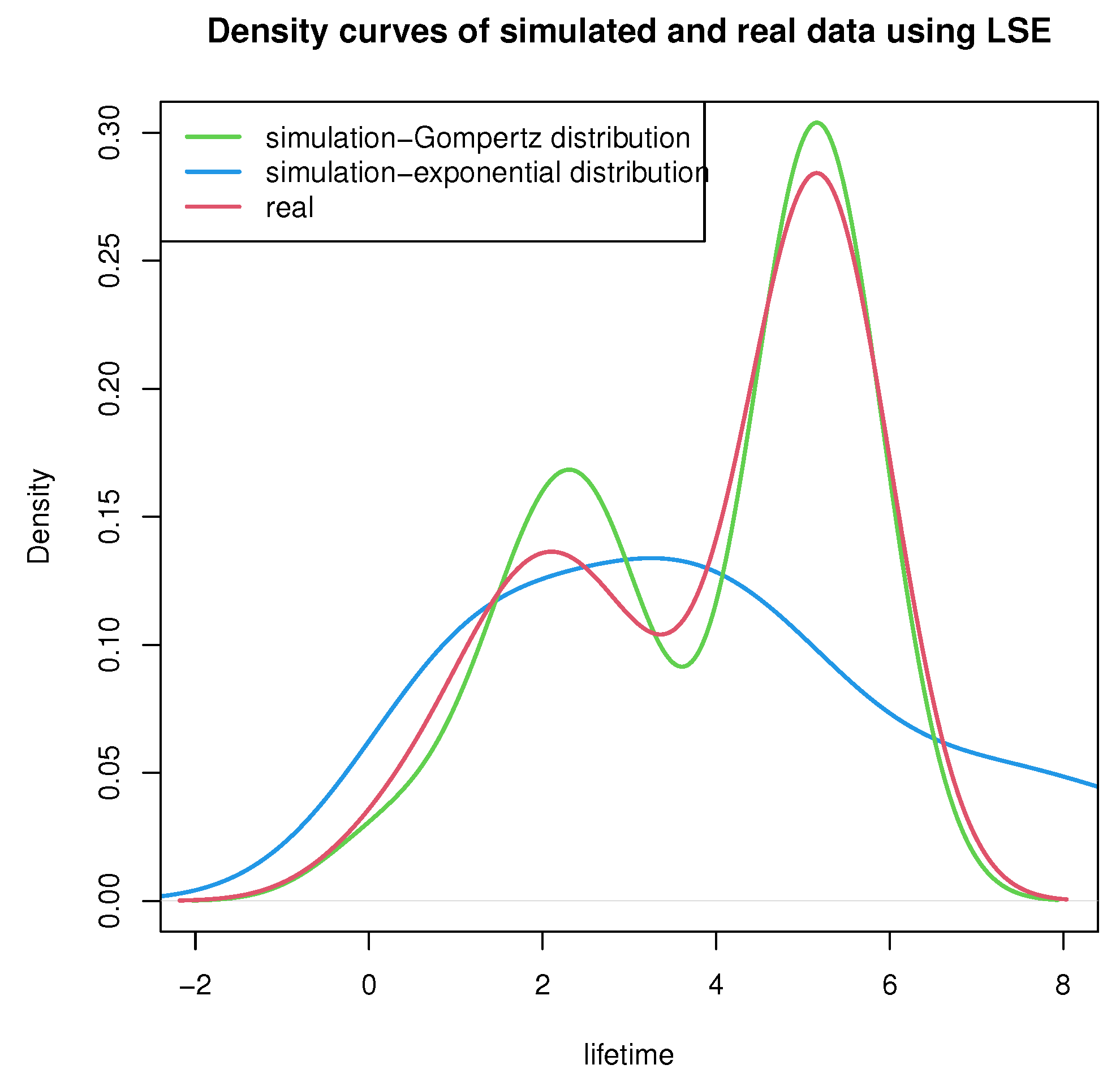
In order to show that the Gompertz distribution has good properties in solving such models, we make statistical inferences using the same methods when the lifetime distribution obeys the exponential distribution under the proposed model and assumptions. Moreover, we compare the results under Gompertz distribution and exponential distribution. Part C of Section 1 states that Gompertz distribution with two parameters degenerates to the exponential distribution with one parameter, as scale parameter λ tends to zero. Thus, by making λ 1 and λ 2 equal to 0.001, the distribution is considered to obey exponential distribution. The density curves of simulated and real data using MLE and LSE based on the Gompertz and exponential distributions are shown in Figure 5 and Figure 6.
Based on the real dataset, the results of ACI and BPI at 90 % , 95 % and 99 % confidence levels are shown in Table 15.
By examining the fitting curves of maximum likelihood estimation and least square estimation, it was observed that the fitting effect of the two point estimation methods is satisfactory, the lengths of the ACI and BPI are approximately equal and the two point estimation values fall into the range of the confidence intervals.

9. Discussion

In this paper, we assume that the hazard function of the lag period is only related to the stress level and is linear with time. If the assumption about the lag period being linear does not hold. The lag period and the subsequent time will be modeled mistakenly. In practice, an assessment of model can help researchers determine if the chosen method is appropriate. Thus, we need to test the hypothesis about the lag period. For nuisance factors, they are classified into three categories in Ref. [28] as uncontrollable and unknown, uncontrollable and known and controllable and known. For the uncontrollable and unknown nuisance factors, randomization is used by increasing the sample size of the experiment to eliminate the effect. For the uncontrollable and known nuisance factors, it is handled by calculating the covariance. For controllable and known nuisance factors, blocks are conducted for experiments. Considering hypothesis tests where the lags are modeled as linear, Ref. [29] suggested performing repeated counting and sensitivity analysis to assess the impact of these different inputs.
In our study, all cases can benefit from independently modeling competing risks, except for the strong dependencies between risks. In many cases where dependencies between risks are not considered, reliable conclusions can be drawn, and tedious calculations can be eliminated, which is important in engineering and in practical applications. In practice, some causes do not always satisfy this independence assumption. Considering the dependence structure between competing risks, binary or multivariate distributions can be used to describe the dependence between failure causes. For example, Refs. [30,31,32] used Marshall–Olkin type distribution, Moran–Downton exponential distribution and copula models, respectively, to describe this binary or multivariate relationship. In subsequent studies, we will also carefully consider the impact on this model when risk factors are not independent.

10. Conclusions

The cumulative risk model more realistically reflects the impact of stress changes and addresses the main constraint of existing models. The Gompertz distribution model is a common model used in reliability and life testing and has two parameters and has many satisfactory properties. Taking into account competing risks, the Gompertz cumulative risk model is an extremely flexible step-stress model and is suitable for many applications in survivability analysis.
In this paper, the parameters estimation problems of the step-stress ALT model considering lagged effect and competing risks are studied. The maximum likelihood method and least squares method are used to determine point estimates. The Newton–Raphson algorithm was used to solve the nonlinear equations. The asymptotic confidence intervals and percentile bootstrap confidence intervals are constructed. From the numerical simulation, it can be observed that, with an increased sample size n, the estimates of both maximum likelihood estimation and least squares estimation converge to the true values, and the mean square errors gradually reduce and tend to zero. Moreover, the maximum likelihood estimates are much closer to the true value than the least squares estimates. In interval estimation, with an increasing sample size n, the mean interval lengths of asymptotic confidence intervals and Boot-p confidence intervals become slimmer, and the coverage rates are very close to confidence level ( 1 α ) % . It is also shown that asymptotic confidence intervals have higher coverage rates when estimating λ 1 , λ 2 , and Boot-p confidence intervals have higher coverage rates when estimating β 1 , β 2 . The simulation results also suggest that the Boot-p confidence intervals have stable coverage rates and narrow average interval lengths for small samples. The model proposed in this paper has been shown to be valuable by simulation in estimating parameters. On the basis of theoretical results, the analysis of the real data was carried out to illustrate this model.
Step-stress models with lagged effect and competing risks are more practical and useful in practical survival analysis and deserve further investigation. In this paper, step-stress accelerated life tests with two stress levels and two risks are considered, which can be extended to models with diverse stress levels and various failure risks. For the next research study, we can further explore this in the case where risk factors are not independent and can also research different stress parameters under different competing risks and propose different truncation methods.

Author Contributions

Investigation, Y.M.; Supervision, W.G. All authors have read and agreed to the published version of the manuscript.

Funding

This research was supported by Project 202210004002 which was supported by National Training Program of Innovation and Entrepreneurship for Undergraduates.

Institutional Review Board Statement

Not applicable.

Informed Consent Statement

Not applicable.

Data Availability Statement

The data presented in this study are openly available in Ref. [9].

Conflicts of Interest

The authors declare no conflict of interest.

Appendix A

By using CRM, all units are affected by stress level s 1 in the initial period. At a predetermined time τ 1 , the stress level begins to increase. The improvement in stress level is fully realized at τ 2 and the stress level is up to s 2 . The hazard function h j ( t ) under the Gompertz distribution of the j-th risk factor can be obtained as follows.
h j ( t ) = β j × e λ 1 t 0 < t < τ 1 , a j + b j t τ 1 t < τ 2 , β j × e λ 2 t τ 2 t .
The cumulative hazard function under the proposed CRM model is as follows.
H j ( t ) = β j λ 1 ( e λ 1 t 1 ) 0 < t < τ 1 , β j λ 1 ( e λ 1 τ 1 1 ) + a j ( t τ 1 ) + b j 2 ( t 2 τ 1 2 ) τ 1 t < τ 2 , β j λ 1 ( e λ 1 τ 1 1 ) + a j ( τ 2 τ 1 ) + b j 2 ( τ 2 2 τ 1 2 ) + β j λ 2 ( e λ 2 t e λ 2 τ 2 ) τ 2 t .
With the CEM, the stress level at the initial stage is s 1 . At a predetermined time τ , stress level increases to s 2 . The hazard function h j * ( t ) for the j-th risk factor under the Gompertz distribution is as follows.
h j * ( t ) = β j × e λ 1 t 0 < t < τ , β j × e λ 2 t τ t .
If we assume that the cumulative hazard functions are constant at the stress levels s 1 and s 2 , the cumulative hazard function H j * ( t ) for CEM is as follows.
H j * ( t ) = β j λ 1 ( e λ 1 t 1 ) 0 < t < τ , β j λ 1 ( e λ 1 τ 1 1 ) + β j λ 2 ( e λ 2 t e λ 2 τ 2 ) τ t .
If we let δ = τ 2 τ 1 0 , which means τ 1 = τ 2 , we can observe that CRM converges to the CEM by comparing the hazard function and the cumulative hazard function.

Appendix B

The CDF of lifetime F X ( t ) considering two independent competing factors is as follows.
F X ( t ) = 1 exp ( β 1 + β 2 ) τ 1 ln ( a j + b j τ 1 ) ln β j a j + b j τ 1 β j t τ 1 1 0 < t < τ 1 1 exp ( β 1 + β 2 ) τ 1 ln ( a j + b j τ 1 ) ln β j a j + b j τ 1 β j 1 × exp ( a 1 + a 2 ) t τ 1 ( b 1 + b 2 ) 2 t 2 τ 1 2 τ 1 t < τ 2 , 1 exp ( β 1 + β 2 ) τ 1 ln ( a j + b j τ 1 ) ln β j a j + b j τ 1 β j 1 × exp ( a 1 + a 2 ) τ 2 τ 1 ( b 1 + b 2 ) 2 τ 2 2 τ 1 2 × exp ( β 1 + β 2 ) τ 2 ln ( a j + b j τ 2 ) ln β j a j + b j τ 2 β j t τ 2 a j + b j τ 2 β j τ 2 t .
The probability density function f X ( t ) of lifetime under the two independent competing factors is as follows.
f X ( t ) = ( β 1 + β 2 ) a j + b j τ 1 β j t τ 1 exp ( β 1 + β 2 ) τ 1 ln ( a j + b j τ 1 ) ln β j a j + b j τ 1 β j t τ 1 1 0 < t < τ 1 , ( a 1 + a 2 ) + ( b 1 + b 2 ) t exp ( β 1 + β 2 ) τ 1 ln ( a j + b j τ 1 ) ln β j a j + b j τ 1 β j 1 × exp ( a 1 + a 2 ) t τ 1 ( b 1 + b 2 ) 2 t 2 τ 1 2 τ 1 t < τ 2 , ( β 1 + β 2 ) a j + b j τ 2 β j t τ 2 exp ( β 1 + β 2 ) τ 1 ln ( a j + b j τ 1 ) ln β j a j + b j τ 1 β j 1 × exp ( a 1 + a 2 ) τ 2 τ 1 ( b 1 + b 2 ) 2 τ 2 2 τ 1 2 × exp ( β 1 + β 2 ) τ 2 ln ( a j + b j τ 2 ) ln β j a j + b j τ 2 β j t τ 2 a j + b j τ 2 β j τ 2 t .
Considering two independent competing risks, the joint probability density function f X , C ( t , j ) of lifetime and failure cause is as follows.
f X , C ( t , j ) = β j a j + b j τ 1 β j t τ 1 exp β j τ 1 ln ( a j + b j τ 1 ) ln β j a j + b j τ 1 β j t τ 1 1 × exp β 3 j τ 1 ln ( a 3 j + b 3 j τ 1 ) ln β 3 j a 3 j + b 3 j τ 1 β 3 j t τ 1 1 0 < t < τ 1 , a j + b j t exp a j + b j τ 1 β j τ 1 ln ( a j + b j τ 1 ) ln β j a j t τ 1 b j 2 t 2 τ 1 2 × exp a 3 j + b 3 j τ 1 β 3 j τ 1 ln ( a 3 j + b 3 j τ 1 ) ln β 3 j a 3 j t τ 1 b 3 j 2 t 2 τ 1 2 τ 1 t < τ 2 , β j a j + b j τ 2 β j t τ 2 exp a j + b j τ 1 β j τ 1 ln ( a j + b j τ 1 ) ln β j a j τ 2 τ 1 b j 2 τ 2 2 τ 1 2 × exp β j τ 2 ln ( a j + b j τ 2 ) ln β j a j + b j τ 2 β j t τ 2 a j + b j τ 2 β j × exp a 3 j + b 3 j τ 1 β 3 j τ 1 ln ( a 3 j + b 3 j τ 1 ) ln β 3 j a 3 j τ 2 τ 1 b 3 j 2 τ 2 2 τ 1 2 × exp β j τ 2 ln ( a 3 j + b 3 j τ 2 ) ln β 3 j a 3 j + b 3 j τ 2 β 3 j t τ 2 a 3 j + b 3 j τ 2 β 3 j τ 2 t .

Appendix C

The concrete equations about MLEs are as follows.
l β 1 = n 1 β 1 I i = 1 e λ 1 t i 1 λ 1 I i = 2 e λ 1 τ 1 1 λ 1 + τ 2 e λ 1 τ 1 τ 1 e λ 2 τ 2 τ 2 τ 1 ( t i τ 1 ) + e λ 2 τ 2 e λ 1 τ 1 τ 2 τ 1 t i 2 τ 1 2 2 I i = 3 e λ 1 τ 1 1 λ 1 + τ 2 e λ 1 τ 1 τ 1 e λ 2 τ 2 + ( e λ 2 τ 2 e λ 1 τ 1 ) τ 1 + τ 2 2 + e λ 2 t i e λ 2 τ 2 λ 2 = 0 , l β 2 = n 2 β 2 I i = 1 e λ 1 t i 1 λ 1 I i = 2 e λ 1 τ 1 1 λ 1 + τ 2 e λ 1 τ 1 τ 1 e λ 2 τ 2 τ 2 τ 1 ( t i τ 1 ) + e λ 2 τ 2 e λ 1 τ 1 τ 2 τ 1 t i 2 τ 1 2 2 I i = 3 e λ 1 τ 1 1 λ 1 + τ 2 e λ 1 τ 1 τ 1 e λ 2 τ 2 + ( e λ 2 τ 2 e λ 1 τ 1 ) τ 1 + τ 2 2 + e λ 2 t i e λ 2 τ 2 λ 2 = 0 , l λ 1 = I i = 1 t i + I i = 2 ( τ 2 t i ) τ 1 e λ 1 τ 1 ( τ 2 e λ 1 τ 1 τ 1 e λ 2 τ 2 ) + ( e λ 2 τ 2 e λ 1 τ 1 ) t i ( β 1 + β 2 ) I i = 1 t i λ 1 e λ 1 t i e λ 1 t i + 1 λ 1 2 ( β 1 + β 2 ) I i = 2 τ 1 λ 1 e λ 1 τ 1 e λ 1 τ 1 + 1 λ 1 2 + τ 1 τ 2 ( t i τ 1 ) τ 2 τ 1 e λ 1 τ 1 τ 1 ( t i 2 τ 1 2 ) 2 ( τ 2 τ 1 ) e λ 1 τ 1 ( β 1 + β 2 ) I i = 3 τ 1 λ 1 e λ 1 τ 1 e λ 1 τ 1 + 1 λ 1 2 + τ 1 τ 2 e λ 1 τ 1 τ 1 e λ 1 τ 1 τ 1 + τ 2 2 = 0 , l λ 2 = I i = 3 t i + I i = 2 ( t i τ 1 ) τ 2 e λ 2 τ 2 ( τ 2 e λ 1 τ 1 τ 1 e λ 2 τ 2 ) + ( e λ 2 τ 2 e λ 1 τ 1 ) t i ( β 1 + β 2 ) I i = 2 τ 1 τ 2 ( t i τ 1 ) τ 2 τ 1 e λ 2 τ 2 + τ 2 ( t i 2 τ 1 2 ) 2 ( τ 2 τ 1 ) e λ 2 τ 2 ( β 1 + β 2 ) I i = 3 ( λ 2 t i 1 ) e λ 2 t i ( λ 2 τ 2 1 ) e λ 2 τ 2 λ 2 2 τ 1 τ 2 e λ 2 τ 2 + τ 2 e λ 2 τ 2 τ 1 + τ 2 2 = 0 .

Appendix D

The elements of the observed Fisher information matrix are shown below.
A 11 = n 1 β 1 2 , A 22 = n 2 β 2 2 , A 12 = A 21 = 0 , A 13 = ( n 2 + n 3 ) τ 1 λ 1 e λ 1 τ 1 e λ 1 τ 1 + 1 λ 1 2 + n 3 τ 1 τ 2 e λ 1 τ 1 τ 1 e λ 1 τ 1 τ 1 + τ 2 2 + I i = 1 t i λ 1 e λ 1 τ 1 e λ 1 t i + 1 λ 1 2 + I i = 2 τ 1 τ 2 ( t i τ 1 ) τ 2 τ 1 e λ 1 τ 1 τ 1 ( t i 2 τ 1 2 ) 2 ( τ 2 τ 1 ) e λ 1 τ 1 = A 31 = A 23 = A 32 , A 14 = I i = 2 τ 1 τ 2 ( t i τ 1 ) τ 2 τ 1 e λ 2 τ 2 + τ 2 ( t i 2 τ 1 2 ) 2 ( τ 2 τ 1 ) e λ 2 τ 2 + I i = 3 ( λ 2 t i 1 ) e λ 2 t i ( λ 2 τ 2 1 ) e λ 2 τ 2 λ 2 2 + n 3 τ 1 τ 2 e λ 2 τ 2 + τ 2 e λ 2 τ 2 τ 1 + τ 2 2 = A 41 = A 24 = A 42 , A 33 = I i = 2 τ 1 2 ( t i τ 1 ) ( τ 2 t i ) e λ 1 τ 1 + λ 2 τ 2 [ ( τ 2 t i ) e λ 1 τ 1 + ( t i τ 1 ) e λ 2 τ 2 ] 2 + ( β 1 + β 2 ) I i = 1 ( t i 2 λ 1 2 2 t i λ 1 + 2 ) e λ 1 t i 2 λ 1 3 + ( β 1 + β 2 ) I i = 2 τ 2 τ 1 2 ( t i τ 1 ) τ 2 τ 1 e λ 1 τ 1 τ 1 2 ( t i 2 τ 1 2 ) 2 ( τ 2 τ 1 ) e λ 1 τ 1 + ( β 1 + β 2 ) ( n 2 + n 3 ) ( τ 1 2 λ 1 2 2 τ 1 λ 1 + 2 ) e λ 1 τ 1 2 λ 1 3 + n 3 τ 1 2 τ 2 e λ 1 τ 1 τ 1 2 ( τ 1 + τ 2 ) 2 e λ 1 τ 1 , A 34 = I i = 2 τ 1 τ 2 ( t i τ 1 ) ( τ 2 t i ) e λ 1 τ 1 + λ 2 τ 2 [ ( τ 2 t i ) e λ 1 τ 1 + ( t i τ 1 ) e λ 2 τ 2 ] 2 , A 44 = I i = 2 τ 2 2 ( t i τ 1 ) ( τ 2 t i ) e λ 1 τ 1 + λ 2 τ 2 [ ( τ 2 t i ) e λ 1 τ 1 + ( t i τ 1 ) e λ 2 τ 2 ] 2 + ( β 1 + β 2 ) I i = 2 τ 1 τ 2 2 ( t i τ 1 ) τ 2 τ 1 e λ 2 τ 2 + τ 2 2 ( t i 2 τ 1 2 ) 2 ( τ 2 τ 1 ) e λ 2 τ 2 + ( β 1 + β 2 ) I i = 3 ( t i 2 λ 2 2 2 t i λ 2 + 2 ) e λ 2 t i ( τ 2 2 λ 2 2 2 τ 2 λ 2 + 2 ) e λ 2 τ 2 λ 2 3 + ( β 1 + β 2 ) n 3 τ 2 2 τ 1 e λ 2 τ 2 + τ 2 2 ( τ 1 + τ 2 ) 2 e λ 2 τ 2 .

References

  1. Han, D.; Balakrishnan, N. Inference for a simple step-stress model with competing risks for failure from the exponential distribution under time constraint. Comput. Stat. Data Anal. 2010, 54, 2066–2081. [Google Scholar] [CrossRef]
  2. Aljohani, H.M.; Alfar, N.M. Estimations with step-stress partially accelerated life tests for competing risks Burr XII lifetime model under type-II censored data. Alex. Eng. J. 2020, 59, 1171–1180. [Google Scholar] [CrossRef]
  3. Kannan, N.; Kundu, D. Weibull Step-Stress Model with a Lagged Effect. Am. J. Math. Manag. Sci. 2018, 37, 33–50. [Google Scholar] [CrossRef]
  4. Beltrani, J. Weibull lagged effect step-stress model with competing risks. Commun. Stat.—Theory Methods 2016, 46, 5419–5442. [Google Scholar] [CrossRef]
  5. Wu, M.; Shi, Y. Statistical analysis of dependent competing risks model from Gompertz distribution under progressively hybrid censoring. SpringerPlus 2016, 5, 1745. [Google Scholar]
  6. Crowder, M.J. On the identifiability crises in competing risks analysis. Scand. J. Stat. 1991, 18, 223–233. [Google Scholar]
  7. Kalbfleisch, J.D.; Prentice, R.L. The Statistical Analysis of Failure Time Data; John Wiley & Sons, Inc.: Hoboken, NJ, USA, 2002. [Google Scholar]
  8. Kundu, D.; Pradhan, B. Bayesian analysis of progressively censored competing risks data. Sankhya B 2011, 73, 276–296. [Google Scholar] [CrossRef]
  9. Han, D.; Kundu, D. Inference for a Step-Stress Model with Competing Risks for Failure From the Generalized Exponential Distribution Under Type-I Censoring. IEEE Trans. Reliab. 2015, 64, 31–43. [Google Scholar] [CrossRef]
  10. Pascual, F.G. Accelerated Life Test Planning with Independent Weibull Competing Risks. IEEE Trans. Reliab. 2008, 57, 435–444. [Google Scholar] [CrossRef]
  11. Zhang, L.F.; Xie, M.; Tang, L.C. Robust Regression using Probability Plots for Estimating the Weibull Shape Parameter. Qual. Reliab. Eng. Int. 2006, 22, 905–917. [Google Scholar] [CrossRef]
  12. Maller, R.A.; Xian, Z. Analysis of parametric models for competing risks data. Stat. Sin. 2002, 12, 725–750. [Google Scholar]
  13. Sedyakin, N.M. On one physical principle in reliability theory. Tech. Cybernatics 1966, 3, 80–87. [Google Scholar]
  14. Xiao, L.; Wei, S.Q. Modeling and Planning of Step-Stress Accelerated Life Tests with Independent Competing Risks. IEEE Trans. Reliab. 2011, 60, 712–720. [Google Scholar]
  15. Yuan, T.; Liu, X.; Kuo, W. Planning Simple Step-Stress Accelerated Life Tests Using Bayesian Methods. IEEE Trans. Reliab. 2012, 61, 254–263. [Google Scholar] [CrossRef]
  16. Nelson, W. Accelerated Life Testing - Step-Stress Models and Data Analyses. IEEE Trans. Reliab. 1980, 29, 103–108. [Google Scholar] [CrossRef]
  17. Kateri, M.; Kamps, U. Inference in step-stress models based on failure rates. Stat. Pap. 2014, 56, 639–660. [Google Scholar] [CrossRef]
  18. Kundu, D.; Ganguly, A. Analysis of Step-Stress Models: Existing Results and Some Recent Developments; Elsevier Science: San Diego, CA, USA, 2017. [Google Scholar]
  19. Kannan, N.; Kundu, D.; Balakrishnan, N. Chapter Advances in Degradation Modeling. In Survival Models for Step-Stress Experiments with Lagged Effects; Birkhäuser: Boston, MA, USA, 2010; pp. 355–369. [Google Scholar]
  20. Beltrani, J. Exponential competing risk step-stress model with lagged effect. Int. J. Math. Stat. 2015, 16, 1–16. [Google Scholar]
  21. Valkovics, J. The Gompertz distribution and its applications. Genus 1992, 48, 15–28. [Google Scholar]
  22. Makany, R. A Theoretical Basis for Gompertz’S Curve. Biom. J. 1991, 33, 121–128. [Google Scholar] [CrossRef]
  23. Franses, P.H. Fitting a Gompertz Curve. J. Oper. Res. Soc. 1994, 45, 109–113. [Google Scholar] [CrossRef]
  24. Chen, Z. Parameter Estimation of the Gompertz Population. Biom. J. 1997, 39, 117–124. [Google Scholar] [CrossRef]
  25. Almarashi, A.; Abd-Elmougod, G. Accelerated competing risks model from Gompertz lifetime distributions with type-II censoring scheme. Therm. Sci. 2020, 24, 165–175. [Google Scholar] [CrossRef]
  26. Alghamdi, A.S. Partially Accelerated Model for Analyzing Competing Risks Data from Gompertz Population under Type-I Generalized Hybrid Censoring Scheme. Complexity 2021, 2021, 1–12. [Google Scholar] [CrossRef]
  27. Efron, B.; Tibshirani, R.J. An Introduction To The Bootstrap. J. Am. Stat. Assoc. 1993, 89, 436. [Google Scholar]
  28. Montgomery, D.C. Design and Analysis of Experiments; John Wiley & Sons, Inc.: Hoboken, NJ, USA, 1976. [Google Scholar]
  29. Escobar, L.A.; Meeker, W.Q. A Review of Accelerated Test Models. Stat. Sci. 2006, 21, 552–577. [Google Scholar] [CrossRef] [Green Version]
  30. Kundu, D.; Dey, A.K. Estimating the parameters of the Marshall-Olkin bivariate Weibull distribution by EM algorithm. Comput. Stat. Data Anal. 2009, 53, 956–965. [Google Scholar] [CrossRef] [Green Version]
  31. Iliopoulos, G. Estimation of parametric functions in Downton’s bivariate exponential distribution. J. Stat. Plan. Inference 2003, 117, 169–184. [Google Scholar] [CrossRef] [Green Version]
  32. Wu, M.; Shi, Y.; Zhang, C. Statistical analysis of dependent competing risks model in accelerated life testing under progressively hybrid censoring using copula function. Commun. Stat. Simul. Comput. 2015, 4, 4004–4017. [Google Scholar] [CrossRef]
Figure 1. PDF of Gompertz distribution.
Mathematics 09 03206 g001
Figure 2. CDF of Gompertz distribution.
Mathematics 09 03206 g002
Figure 3. Trace plot of MLE for β 1 .
Mathematics 09 03206 g003
Figure 4. Trace plot of LSE for β 1 .
Mathematics 09 03206 g004
Figure 5. Density curves of simulated and real data using MLE.
Mathematics 09 03206 g005
Figure 6. Density curves of simulated and real data using LSE.
Mathematics 09 03206 g006
Table 1. The point estimation results using MLE and LSE under True Value I.
β ^ 1 β ^ 2 λ ^ 1 λ ^ 2
n MethodMeanMSEMeanMSEMeanMSEMeanMSE
25MLE0.21430.38630.11050.14110.08142.77850.23600.5084
50MLE0.20560.09040.10270.02700.09190.67400.2180.1191
75MLE0.20570.04090.10210.01260.09560.30010.21000.0471
100MLE0.20220.02090.10160.00700.09920.15640.20900.0274
200MLE0.20250.00600.10060.00190.09990.04190.20260.0064
500MLE0.19960.00090.10030.00030.10180.00640.20290.0011
25LSE0.27900.46340.14270.1825----
50LSE0.24690.08320.12070.0269----
75LSE0.23300.03000.11690.0116----
100LSE0.22550.01440.11290.0057----
200LSE0.21390.00310.10790.0012----
500LSE0.20710.00040.10340.0002----
Table 2. The point estimation results using MLE and LSE under True Value II.
β ^ 1 β ^ 2 λ ^ 1 λ ^ 2
n MethodMeanMSEMeanMSEMeanMSEMeanMSE
25MLE0.16020.27610.10840.14700.09973.08120.23190.4705
50MLE0.15570.05950.10320.02790.09560.69630.21550.0984
75MLE0.15340.02660.10250.01290.09890.30720.20960.0419
100MLE0.15290.01540.10180.00750.09860.18660.20750.0227
200MLE0.14980.00390.10030.00190.10320.04550.20440.0064
500MLE0.15040.00060.10000.00030.10180.00720.20180.0010
25LSE0.21110.28790.13930.1498----
50LSE0.18460.05020.12210.0265----
75LSE0.17400.01780.11670.0101----
100LSE0.16850.00850.11180.0047----
200LSE0.16140.00190.10770.0010----
500LSE0.15500.00020.10360.0001----
Table 3. The point estimation results using MLE and LSE under True Value III.
β ^ 1 β ^ 2 λ ^ 1 λ ^ 2
n MethodMeanMSEMeanMSEMeanMSEMeanMSE
25MLE0.21470.36840.10740.11250.09441.45070.25360.8353
50MLE0.20440.07840.10250.02740.10560.3640.22430.1428
75MLE0.20490.03230.10260.01100.09380.15540.21370.0494
100MLE0.20210.01800.10030.00600.10240.08620.20960.0281
200MLE0.20110.00480.10080.00140.09990.02250.2040.0069
500MLE0.19940.00070.09980.00020.10360.00330.20320.0011
25LSE0.27860.44640.13880.1561----
50LSE0.24750.08770.12360.0299----
75LSE0.23400.03280.11600.0110----
100LSE0.22550.01420.11160.0049----
200LSE0.21440.00310.10790.0012----
500LSE0.20680.00040.10370.0002----
Table 4. The point estimation results using MLE and LSE under True Value IV.
β ^ 1 β ^ 2 λ ^ 1 λ ^ 2
n MethodMeanMSEMeanMSEMeanMSEMeanMSE
25MLE0.16090.22580.10590.12410.09411.72930.23210.4815
50MLE0.15460.04970.10360.02690.09660.39050.21890.1031
75MLE0.15210.02170.10100.01090.10420.17140.20880.0407
100MLE0.15130.01300.10020.00590.10270.09940.20900.0235
200MLE0.15110.00280.10060.00150.09990.02180.20320.0054
500MLE0.15070.00050.10010.00020.10010.00360.20070.0009
25LSE0.21010.26580.13570.1262----
50LSE0.18390.04570.12270.0266----
75LSE0.17620.01960.11710.0110----
100LSE0.16900.00830.11330.0055----
200LSE0.16150.00200.10680.0010----
500LSE0.15500.00020.10340.0001----
Table 5. Mean lengths and coverage rates using ACI and BPI at 95 % CL under True Value I.
Asymptotic Confidence IntervalBoot-p Confidence Interval
n β 1 β 2 λ 1 λ 2 β 1 β 2 λ 2 λ 2
25ML0.37630.21480.59610.38750.39640.22461.07490.441
CR0.9190.9000.9670.9550.9400.9300.9600.930
50ML0.25150.14280.43480.27730.26020.14850.71060.2788
CR0.9160.9190.9490.9450.9500.9300.9400.900
75ML0.19900.11400.37050.22670.20290.11460.56190.2280
CR0.9180.9140.9460.9350.9300.9000.8900.890
100ML0.16830.09690.34000.19650.17740.10340.48750.1914
CR0.9260.9270.9470.9440.9200.9300.9200.920
200ML0.11710.06790.25890.13680.12510.07100.33570.1336
CR0.9080.9250.9400.9390.8900.9200.9000.890
500ML0.07320.04240.18820.08580.07930.04450.21340.0850
CR0.9210.9190.9350.9470.9200.9200.9400.910
Table 6. Mean lengths and coverage rates using ACI and BPI at 99 % CL under True Value I.
Asymptotic Confidence IntervalBoot-p Confidence Interval
n β 1 β 2 λ 1 λ 2 β 1 β 2 λ 2 λ 2
25ML0.48780.26270.76210.48730.50350.30881.34500.6192
CR0.9530.9470.9950.9870.9900.9900.9900.980
50ML0.32660.18750.55720.35730.32800.19300.88330.3533
CR0.9580.9480.9890.9820.9800.9700.9900.910
75ML0.26030.14940.46670.29380.25840.14630.71030.2837
CR0.9600.9670.9850.9870.9900.9800.9800.960
100ML0.22170.12770.41660.25520.22870.12970.60930.2412
CR0.9680.9620.9860.9900.9700.9800.9400.970
200ML0.15410.08930.32390.18020.15530.08850.42660.1666
CR0.9800.9720.9910.9910.9900.9900.9700.980
500ML0.09640.05600.23310.11290.09480.05370.26430.1055
CR0.9780.9770.9810.9890.9600.9800.9900.940
Table 7. Mean lengths and coverage rates using ACI and BPI at 95 % CL under True Value II.
Asymptotic Confidence IntervalBoot-p Confidence Interval
n β 1 β 2 λ 1 λ 2 β 1 β 2 λ 2 λ 2
25ML0.29320.20630.61540.36490.29390.20881.15760.4343
CR0.8840.8720.9480.9530.9400.9100.9200.860
50ML0.18980.13650.45290.25540.20950.15160.73860.2706
CR0.9010.8860.9460.9330.9200.9100.9400.860
75ML0.15200.10930.37500.20540.16660.11940.59890.2185
CR0.8910.8820.9270.9360.9000.8700.8900.870
100ML0.13050.09470.33600.17660.14390.1000.50870.1845
CR0.9000.9290.9460.9400.9300.8800.9400.900
200ML0.09020.06550.26360.12350.10160.07170.36000.1280
CR0.8990.9090.9550.9280.9400.9200.9300.960
500ML0.05610.04070.19260.07760.06240.04470.21740.0808
CR0.8980.9290.9490.9210.8300.8800.8400.920
Table 8. Mean lengths and coverage rates using ACI and BPI at 99 % CL under True Value II.
Asymptotic Confidence IntervalBoot-p Confidence Interval
n β 1 β 2 λ 1 λ 2 β 1 β 2 λ 2 λ 2
25ML0.34800.24930.80250.46540.40760.31061.45900.5345
CR0.9230.9230.9880.9920.9800.9700.9900.960
50ML0.25310.18560.56430.33000.27400.19440.95550.3341
CR0.9480.9440.9910.9800.9800.9700.9900.980
75ML0.19780.14280.48370.27020.21320.14650.74470.2644
CR0.9460.9470.9820.9840.9800.9700.9700.970
100ML0.17020.12340.42560.23190.18170.12780.64820.2303
CR0.9640.9690.9850.9860.9700.9900.9700.980
200ML0.11830.08560.32590.16220.12590.08780.44300.1591
CR0.9620.9650.9830.9830.9800.9700.9900.960
500ML0.07420.05370.23650.10190.07880.05580.27290.0999
CR0.9670.9710.9850.9770.9900.9700.9900.980
Table 9. Mean lengths and coverage rates using ACI and BPI at 95 % CL under True Value III.
Asymptotic Confidence IntervalBoot-p Confidence Interval
n β 1 β 2 λ 1 λ 2 β 1 β 2 λ 2 λ 2
25ML0.34600.20020.47170.40290.35060.20500.77080.5258
CR0.9180.9130.9640.9080.9300.9500.9500.900
50ML0.22550.13350.35410.29020.24070.13560.52370.3177
CR0.9110.9150.9410.9240.9400.9700.9500.870
75ML0.17810.10530.30390.23400.18980.10860.41630.2433
CR0.9090.9140.9570.9390.9300.9300.9500.920
100ML0.15320.09050.27370.20310.15990.0950.35040.2084
CR0.9280.9310.9480.9450.9300.9100.9000.860
200ML0.10540.06280.21830.14210.11210.06490.25170.1414
CR0.9130.9390.9580.9450.9300.9600.9600.850
500ML0.06640.03960.15480.08850.07110.04100.15740.0882
CR0.9340.9250.9580.9400.9100.9400.9500.910
Table 10. Mean lengths and coverage rates using ACI and BPI at 99 % CL under True Value III.
Asymptotic Confidence IntervalBoot-p Confidence Interval
n β 1 β 2 λ 1 λ 2 β 1 β 2 λ 2 λ 2
25ML0.42820.23450.60520.50610.4350.26080.97940.8264
CR0.9460.9480.9920.9720.9900.9800.9700.960
50ML0.29430.17480.44530.37100.30420.17490.65850.4182
CR0.9620.9590.9860.9750.9900.9600.9600.970
75ML0.23330.13930.37900.30580.23780.14070.51670.3052
CR0.9670.9660.9930.9810.9800.9700.9900.930
100ML0.19940.11870.34260.26720.19740.11540.45230.2602
CR0.9610.9630.9870.9840.9700.9800.9900.920
200ML0.13900.08290.26590.18570.13910.08180.30730.1760
CR0.9720.9750.9920.9820.9700.9600.9800.980
500ML0.08700.05180.19580.11670.08890.05110.19910.1089
CR0.9750.9760.9880.9860.9900.9900.9700.960
Table 11. Mean lengths and coverage rates using ACI and BPI at 95 % CL under True Value IV.
Asymptotic Confidence IntervalBoot-p Confidence Interval
n β 1 β 2 λ 1 λ 2 β 1 β 2 λ 2 λ 2
25ML0.25810.18360.48530.36370.26660.19300.79410.4553
CR0.8760.8780.9540.9230.9100.9300.9200.880
50ML0.16830.12330.36140.25250.19080.13790.54030.2726
CR0.9000.8900.9440.9370.9400.9000.9400.860
75ML0.13630.09980.30710.20410.14610.10560.42990.2176
CR0.8960.8950.9440.9360.9000.8500.8900.900
100ML0.11640.08620.27970.17710.12760.09360.36470.1813
CR0.8850.9090.9440.9170.9200.9300.9300.930
200ML0.08120.06000.21620.12220.09070.06330.25740.1278
CR0.8980.9090.9490.9280.9400.8900.9400.940
500ML0.05080.03760.15660.07700.05750.04220.16140.0791
CR0.9120.9250.9590.9340.9200.9600.9200.920
Table 12. Mean lengths and coverage rates using ACI and BPI at 99 % CL under True Value IV.
Asymptotic Confidence IntervalBoot-p Confidence Interval
n β 1 β 2 λ 1 λ 2 β 1 β 2 λ 2 λ 2
25ML0.32550.22790.61410.45430.36570.25981.03960.6015
CR0.9210.9160.9910.9830.9800.9600.9500.950
50ML0.22020.16210.45570.32930.24430.16880.67030.3427
CR0.9530.9610.9900.9880.9600.9900.9500.920
75ML0.18020.13090.38090.26830.19230.13750.52640.2747
CR0.9520.9640.9890.9900.9900.9900.9800.980
100ML0.15200.11150.34790.23130.16140.11530.46460.2291
CR0.9530.9530.9800.9860.9500.9900.9500.960
200ML0.10640.07850.27010.16160.11390.08140.31830.1587
CR0.9640.9670.9930.9870.9800.9800.9800.950
500ML0.06670.04920.19740.10130.07090.05060.19630.0992
CR0.9730.9710.9900.9800.9700.9700.9900.950
Table 13. Lifetime data of solar lighting devices on step-stress ALT considering lagged effect.
Stess Level S1LaggedStess Level S1
Failure TimeFailure FactorFailure TimeFailure FactorFailure TimeFailure Factor
0.14014.89225.2381
0.78325.00215.2441
1.32425.02225.2471
1.58215.08225.3051
1.71625.11215.3372
1.79425.14715.4071
1.8832 5.4082
2.2932 5.4451
2.6602 5.4831
2.6742 5.7172
2.7252
3.0852
3.9422
4.3962
4.6121
Table 14. Estimation results using MLE and LSE.
β 1 β 2 λ 1 λ 2
MLE0.04040.0560.13320.6631
LSE0.05340.074--
Table 15. Interval estimation results of β 1 , β 2 , λ 1 and λ 2 on the real dataset.
ParameterCLAsymptotic Confidence IntervalBoot-p Confidence Interval
β 1 90%(0.0137, 0.0671)(0.0102, 0.0932)
95%(0.0086, 0.0723)(0.0091, 0.0966)
99%(0.0000, 0.0823)(0.0077, 0.1011)
β 2 90%(0.0215, 0.0904)(0.0154, 0.1279)
95%(0.0149, 0.0970)(0.0128, 0.1335)
99%(0.0020, 0.1099)(0.0149, 0.1744)
λ 1 90%(0.0000, 0.4201)(−0.2373, 0.5100)
95%(0.0000, 0.4751)(−0.2593, 0.5993)
99%(0.0000, 0.5825)(−0.6138, 0.5202)
λ 2 90%(0.5309, 0.7953)(0.4952, 0.8991)
95%(0.5056, 0.8206)(0.4896, 0.9605)
99%(0.4561, 0.8701)(0.4880, 0.9180)
Publisher’s Note: MDPI stays neutral with regard to jurisdictional claims in published maps and institutional affiliations.

