On the Quantitative Properties of Some Market Models Involving Fractional Derivatives

Abstract

We review and discuss the properties of various models that are used to describe the behavior of stock returns and are related in a way or another to fractional pseudo-differential operators in the space variable; we compare their main features and discuss what behaviors they are able to capture. Then, we extend the discussion by showing how the pricing of contingent claims can be integrated into the framework of a model featuring a fractional derivative in both time and space, recall some recently obtained formulas in this context, and derive new ones for some commonly traded instruments and a model involving a Riesz temporal derivative and a particular case of Riesz–Feller space derivative. Finally, we provide formulas for implied volatility and first- and second-order market sensitivities in this model, discuss hedging and profit and loss policies, and compare with other fractional (Caputo) or non-fractional models.

1. Introduction

1.1. Stock Returns and Tempered Stable Lévy Processes

Modeling the behavior of stock returns is a deep and fascinating question, which has been studied by several fields of science for over a hundred years now. Historically, the randomness of market returns was initially conceptualized from a probabilistic perspective, with the pioneering works of Bachelier [1] (normal hypothesis) and Black, Scholes, and Merton [2,3] (log-normal hypothesis). It was later extended to take into account other characteristics such as non-constant volatility [4] or existence of jumps [5] for instance. During the past 30 years, this probabilistic setup has been completed by several new approaches utilizing tools from statistical physics, such as dynamical (chaotic) systems, thermodynamics [6], fractals and multi-fractals [7,8], gas theory [9], or complex networks [10]. Such methods are often referred to as the econophysics approach to financial modeling, a broad discipline to which the reader will find a complete introduction in the classical monograph [11].

Particularly important in econophysics is the theory of truncated Lévy flights. These processes have been introduced in [12] for their physically attractive features, such as the existence of the second moment (variance) or the transition to a Gaussian process after a (possibly very high) number of independent events. They were formalized in terms of their characteristic function in the symmetric case [13], and, some years later, they were generalized to asymmetric distributions and introduced in quantitative finance under the name of CGMY (Carr–Geman–Madan–Yor) [14], KoBoL [15], or tempered stable Lévy processes [16].

The popularity that tempered stable Lévy processes have achieved in financial modeling stems from their ability to capture phenomena that the log-normal assumption, which underlies the traditional Black–Scholes–Merton model, fails to describe. Among these phenomena, the presence of extreme events (price jumps) whose existence has been assessed once again during the COVID-19 crisis. Let us consider, for instance, the Dow Jones Industrial Average and the Standard and Poor’s 500 indices, which lost respectively 2000 points and 7.6% on 9 March 2020, or the London Stock Exchange “Footsie” index that lost 10.87% on 12 March 2020. If stock returns (or, as customary considered in quantitative finance, stock log returns) were normally distributed, the existence of such events with non-zero probability would be prevented by the absence of excess kurtosis in the distribution.

Alongside jumps, tempered stable processes also capture the asymmetry of the distributions (price drops occur more often than prise rise) or the fact that volatility is not constant over time. Some tempered stable processes, such as the Variance Gamma process [17] even allow for an interpretation as a time changed Brownian motion, that is, traduce the fact that the business time driving the market differs from the physical time. A recent example of such behavior includes, for instance, the “flash crash” of 6 May 2010: The Dow Jones Index lost 9% in approximately 30 min, and a large part of the loss was recovered later that day.

1.2. Why Fractional Operators Arise

There is a strong connection between tempered stable Lévy processes and fractional calculus because, under such models, probability densities and option prices satisfy a fractional partial differential equation involving a Riemann–Liouville or a Riesz–Feller derivative [18,19,20,21] in the space variable [15,22]. Moreover, as these derivatives nest the usual local derivatives when their order is an integer, these equations generalize the traditional equations encountered in the Black–Scholes–Merton framework (parabolic partial differential equation for the European option, which reduces to the heat equation for the Gaussian density). Moreover, in some cases, the order of the space-fractional derivative has a direct interpretation in terms of excess kurtosis for the distribution of returns [23], and of the magnitude of the model’s randomness [7]. This remarkable connection between fractional calculus and financial modeling arises notably because the Riesz–Feller derivative is a pseudo-differential operator whose symbol coincides with the infinitesimal generator of the characteristic function of the Lévy-stable process [24,25].

Given the importance of space fractional derivatives, it is legitimate to wonder if time-fractional derivatives can capture interesting features of market returns as well—and the answer is yes. The first pricing formula involving a fractional temporal derivative in the Caputo sense was most likely proved in [26], for a model incorporating a distribution for the arrival of intraday trades (“tick by tick” data) and for the waiting time (“duration”) between them. This approach is similar to the subordination method first introduced by [27], and later developed in models based on time changed Brownian motion [28], or random walks subordinated to renewal processes [29]: All these models, indeed, aim at understanding stock price dynamics in terms of a business time differing from operational time.

Models have subsequently been developed that incorporate both space and time-fractional derivatives [30,31]. Such models are based on the so-called space-time fractional diffusion equation that generalizes the conventional diffusion equation, and combine the presence of both fat tails (controlled by the order of the space fractional derivative) and the subordination parameter (controlled by the time fractional derivative, instead of the variance of the subordinating time process in the Variance Gamma model [17] for instance). In particular, the order of the temporal derivative determines whether the market is in a slow or fast diffusion regime and enables a risk redistribution between options’ maturities (the fact that short term options become cheaper while long term options become more expensive, a phenomenon one can observe in a period of market stress for instance). Let us also mention that time-fractional derivatives have also been used in the description of dynamic memory [32] and that, recently, other types of time-fractional derivatives have been considered, such as the generalized Hilfer–Prabhakar derivative in [33].

1.3. Pricing Contingent Claims

Contingent claims are financial instruments whose payoff depends on the price trajectory of one (or several) underlying asset(s). A prominent example of contingent claims is the broad family of options, which give their owner the right to buy a certain quantity of some financial asset (a stock, an index, an exchange rate) at a certain price (the option’s strike). The payoff delivered by the option can be determined uniquely by the asset’s terminal price (path-independent option) or depend on its full realization throughout the option’s life (path-dependent instruments). Path independent options include European, digital, power, or log options, for instance, while path-dependent options include American, Asian, or barrier options [34].

Of course, the value of an option depends on the model one chooses for the underlying stock returns. When only space fractional derivative is involved (i.e., in the case of tempered stable processes), Fourier and Fast Fourier transform methods, and their refinements [35,36,37,38] are very popular, notably because most characteristic functions are known under a simple form. Furthermore, when a fractional partial differential equation is available (like for European instruments in the CGMY case), then it can be advantageous to utilize a discretization of the integral operators [22]. As these operators are non-local, the procedure is more subtle than the usual finite difference methods; efficient discretization techniques include, for instance, convolution quadrature schemes such as the ones utilized in [39,40] in the context of phase-field separation (Cahn–Hilliard) models featuring non-local memory effects. Fourier-based methods have also been successfully applied to the analysis of a fractional differential equation: For instance in [41], a time fractional partial differential equation is transformed into a sequence of ordinary differential equations via a Fourier expansion along the space coordinates; Fourier pseudospectral methods have also been used for the analysis of multidimensional partial differential equations [42,43], and homogenization functions have been proposed for the analysis of nonlinear time fractional wave equations [44]. Last, for models based on fractional diffusion in both the space and time coordinates, it is possible to use a Mellin–Barnes representation for the density function [45] and to evaluate the arising complex integrals using an appropriate grid [31].

Recently, a new analytical approach has been proposed for models based on the fractional diffusion equation, when the time-fractional derivative is a Caputo derivative. This technique utilizes a Mellin–Barnes representation for the whole convolution operator (instead of the density only) and its evaluation via residue calculus. It allows to express option prices under the form of fast converging series and has been applied to European options [46], digital options [47], or exotic path independent options [48]. The method has also been successfully implemented in other financial models that do not belong to the tempered stable family [49].

1.4. Contributions of the Paper

In this paper, our objective is two-fold: To propose a review of some existing market models that involve fractional derivative in space and/or time, and to introduce a specific model whose properties had not been explored in details so far in the existing literature. For this particular model, we will focus on establishing analytical tools for option pricing, volatility modeling (in some specific cases), and for measuring porftolio performance. In detail, we investigate and provide details on the following key points:

-

Review the various models in the tempered stable family that involve a fractional derivative in the space and/or time variable, and explain the link between order of fractional derivatives a model properties (state of randomness, time subordination, diffusion regime);

-

By analogy with the probabilistic approach, define the fundamental concepts needed for option pricing (convexity adjustement, risk-neutral expectation) in the context of a space-time diffusion;

-

Focus on a fractional diffusion model involving a Riesz time fractional derivative, and establish closed form expression for the convexity adjustment and the price of several options (European, digital, power, log). These formulas are new and come as a complement to the formulas previously obtained in the case of a Caputo time fractional derivative;

-

Derive closed form expression for at-the-money implied volatility and market sensitivities, and deduce some practical considerations for hedging policies and profit and loss of portfolios.

1.5. Structure of the Paper

In Section 2 we will recall some theoretical aspects of Lévy processes and option pricing that will be needed for the rest of the paper. Then, in Section 3, we will introduce the class of a tempered stable Lévy process, showing why these processes are strongly linked to several types of spatial fractional derivatives, and discuss their main features and properties. We will extend this approach in Section 4 by letting the time derivative be fractional as well in the equation governing the densities, and, focusing on a Riesz temporal derivative, establish a factorized formula for the price of an arbitrary path independent claim under this model. Specifying this formula to usual payoff functions and using residue calculus will allow us to obtain, in Section 5, the price of several commonly traded contracts. In Section 6 we will provide some practical tools for the determination of implied volatility and market sensitivity (Delta and Gamma) and discuss how the presence of fractional derivatives affects the hedging policy and profit and loss of strategies; we will also compare the results with other fractional or non-fractional models. Section 7 will be dedicated to conclusive remarks, while main notations and main properties of special functions are summarized in Appendix A and Appendix B respectively.

2. Principles of Option Pricing with Exponential Lévy Motions

Let us start by recalling some essential principles on Lévy processes and some practical details regarding their implementation for option pricing purposes. For more details regarding theoretical details on Lévy processes and their financial applications, we refer to the classical monographs [50,51,52].

2.1. Basics of Lévy Processes

Recall that, given a filtered probability space, a Lévy process, $X(t)$, $t\ge 0,$ is a stochastically continuous process with stationary and independent increments, such that $X(0)=0$ almost surely. Such a process is often specified by its Lévy symbol or characteristic exponent $\psi (\kappa ):=log\mathbb{E}[exp(i\kappa X(1))]$, allowing to express the characteristic function as a one-parameter semigroup:

$$\mathbb{E}\left[e^{i\kappa X(t)}\right]=e^{t\psi (\kappa )},t\ge 0.$$

(1)

The Lévy symbol itself is entirely determined by the Lévy–Khinchine representation theorem, which states that:

$$\psi (\kappa )=ai\kappa -\frac{1}{2}{b}^2{\kappa }^2+\underset{-\infty }{\overset{+\infty }{\int }}\left(e^{i\kappa x}-1-i\kappa x{\mathbb{1}}_{\left\{\right|x|<1\}}\right)\Pi (dx),$$

(2)

where a is the drift and b is the Brownian (or diffusion) component. The measure $\Pi (dx)$, assumed to be concentrated on $\mathbb{R}\setminus \left\{0\right\}$ and to satisfy:

$$\underset{-\infty }{\overset{+\infty }{\int }}\min (1,x^2)\Pi (dx)<\infty$$

is called the Lévy measure of the process, and determines its tail behavior and the distribution of jumps. In detail, when $\Pi (\mathbb{R})<\infty$, one speaks of a process with finite activity (or intensity). This, for instance, is the case of the so-called jump-diffusion processes, whose applications to option pricing include the Kou Model [53] and the Merton model [54]. When $\Pi (\mathbb{R})=+\infty$, one speaks of a process with infinite activity (or intensity), and an infinite number of jumps can occur on any finite time interval; furthermore when $b=0$ then one speaks of a pure jump or purely discontinuous process. Among the most prominent processes with infinite activity are the Finite Moment Log Stable (FMLS) process [23], the Variance Gamma (VG) process [17], and the Normal Inverse Gaussian (NIG) process [55]. Let us also mention that, if $\Pi ({\mathbb{R}}_{-})=0$ (i.e., the Lévy measure is supported by the positive real axis and the process has only upward jumps), one says that the process $X(t)$ is spectrally positive; this is the case of the so-called subordinators, which are almost surely non-decreasing processes. If $-X(t)$ is spectrally positive, then $X(t)$ is said to be spectrally negative (this is, for instance, the case of the FMLS process).

2.2. Exponential Lévy Markets

We assume a filtered probability space $(\Omega ,\mathcal{F},{\left\{{\mathcal{F}}_t\right\}}_{t\ge 0},\mathbb{Q})$ under which valuations are made, and in particular $\mathbb{E}[·]={\mathbb{E}}^{\mathbb{Q}}[·]$. We let $X(t)$ be an arbitrary Lévy process, admitting a Lévy symbol $\psi (\kappa )$.

Assumption 1.

For $T\ge t\ge 0$ and under the measure $\mathbb{Q}$, we assume the stock price model:

$$S(T)=S(t)exp\left((r-q+\omega )\tau +X(\tau )\right),\omega =-\psi (-i),$$

(3)

where $r\in \mathbb{R},q\ge 0$ are the interest and dividend rates, $\tau =T-t$, and $\mathbb{E}\left[e^{X(\tau )}\right]<\infty$.

We note that the so-called convexity adjustment $\omega$ in Assumption 1 ensures that the price process is a $\mathbb{Q}$-martingale, where $\mathbb{E}\left[e^{X(\tau )}\right]=e^{\psi (-i)\tau }<\infty$; it follows that:

$$\mathbb{E}\left[S(T)\right|S(t)]=e^{r\tau }S(t).$$

(4)

For that reason, $\mathbb{Q}$ is often said to be the risk-neutral, or martingale measure. Note that if we assume that $X(t)$ admits a density $f(x,t)$ with respect to the Lebesgue measure, then we can rewrite the convexity adjustment as:

$$\omega =-log\underset{-\infty }{\overset{\infty }{\int }}{e}^{x}f(x,1)dx$$

(5)

which is nothing else than the cumulant generating function evaluated when the Laplace variable p is equal to 1.

Example 1.

If $X(t)=W(t)$ is a Wiener process such that $\mathbb{E}[W(t)]=0$ and $\mathbb{E}\left[W{(t)}^2\right]={\sigma }^{2}t$, then Assumption (1) can be re-written in terms of the stochastic differential equation:

$$\frac{dS(t)}{S(t)}=(r-q)dt+dW(t),t\le T$$

(6)

which is the usual formulation of the Black–Scholes–Merton model$BSM(\sigma )$[2]. In this approach, σ represents the market volatility and quantifies the fluctuations of the price process around its mean. Note that it is well known that:

$$\mathbb{E}\left[e^{i\kappa W(t)}\right]=e^{-t\frac{{(\sigma \kappa )}^2}{2}}$$

(7)

and therefore the Lévy symbol in this specific case is ${\psi }_2(\kappa )=-({\sigma }^2\kappa )/2$, leading to the Gaussian convexity adjustment ${\omega }_2=-{\psi }_2(-i)=-{\sigma }^2/2$ (subscript “2” will be explained later). Let us also remark that the probability density $f(x,\tau )$ of the Wiener process, namely the heat kernel, is known to satisfy the heat equation:

$$\left(\frac{\partial }{\partial \tau }+{\omega }_2\frac{{\partial }^2}{\partial x^2}\right)f(x,\tau )=0$$

(8)

which is the simplest particular case of the fractional model that we will introduce in Section 4.

Last, we recall that the price $\mathcal{C}(t)$ of a contingent claim (e.g., an option) whose payoff $\mathcal{P}$ depends on the terminal market price of the stock price $S(T)$ and, possibly, on other deterministic parameters (such as strike or trigger prices, leverage ratio, etc.) is equal to the expectation of the discounted payoff given the initial price, that is:

$$\mathcal{C}(t)=\mathbb{E}\left[e^{-r\tau }\mathcal{P}(S(T))|S(t)\right].$$

(9)

Equation (9) is often referred to as the risk-neutral, martingale, or arbitrage approach to option pricing (see details in classical references such as [34]). If the process $X(t)$ has a density $f(x,t)$, then, using Assumption 1, one can rewrite the expectation (9) as:

$$\mathcal{C}(t)=e^{-r\tau }\underset{-\infty }{\overset{+\infty }{\int }}\mathcal{P}\left(e^{(r-q+\omega )\tau +x}\right)f(x,\tau )dx.$$

(10)

3. Tempered Stable Processes, Fractional Partial Differential Equations, and Measures of Randomness

Let us now introduce a class of Lévy measures that are of particular interest in financial modeling and, among many interesting properties (time change, magnitude of randomness), illustrate the connection between option pricing and fractional calculus.

3.1. Tempered Stable Densities and Subordination

Tempered Stable (TS) processes have a Lévy measure whose most general form reads:

$$\Pi (dx)=\left[\frac{c_{+}{e}^{-{\lambda }_{+}x}}{x^{1+{\alpha }_{+}}}{\mathbb{1}}_{\{x>0\}}+\frac{c_{-}{e}^{-{\lambda }_{-}\left|x\right|}}{{\left|x\right|}^{1+{\alpha }_{-}}}{\mathbb{1}}_{\{x<0\}}\right]dx,$$

(11)

where $c_{+},c_{-}\in \mathbb{R}$, ${\lambda }_{+},{\lambda }_{-}>0$, and typically, ${\alpha }_{+},{\alpha }_{-}\in (0,2)$. These processes are also known as “truncated Lévy flights” and were constructed by [12,13] originally for a physical purpose in the fully symmetric case ($c_{+}=c_{-}$, ${\lambda }_{+}={\lambda }_{-}$, ${\alpha }_{+}={\alpha }_{-}\ne 1$), and were later considered in capital market modeling and extended to more interesting sub-cases of (11) in CGMY (Carr–Geman–Madan–Yor) [14] or KoBoL [15] models. In particular, in the CGMY formulation, the Lévy measure writes:

$$\Pi (dx)=C\left[\frac{e^{-Mx}}{x^{1+Y}}{\mathbb{1}}_{\{x>0\}}+\frac{e^{-G\left|x\right|}}{{\left|x\right|}^{1+Y}}{\mathbb{1}}_{\{x<0\}}\right]dx$$

(12)

for $C>0$, $G,M\ge 0$, and $Y<2$. Parameter C measures the overall level of activity of the process, while G and M control the exponential tempering of the tails’ decay; the process is symmetric when $G=M$.

Remark 1.

The Lévy symbol for the CGMY model has been derived in [14,15] and can be written:

$$\psi (\kappa )=C\Gamma (Y)\left({(M-i\kappa )}^Y-M^Y+{(G+i\kappa )}^Y-G^Y\right).$$

(13)

The convexity adjustment follows immediately:

$$\omega =-C\Gamma (Y)\left({(M-1)}^Y-M^Y+{(G+1)}^Y-G^Y\right).$$

(14)

Among the most famous CGMY processes, one of the most popular is undoubtedly the Variance Gamma (VG) process [17]. In the VG process, the Y parameter is set to 1, and the other are re-written as:

$$C=\frac{1}{\nu },G=\frac{1}{\sqrt{\frac{{\theta }^2{\nu }^2}{4}+\frac{{\sigma }^2\nu }{2}}+\frac{\theta \nu }{2}},M=\frac{1}{\sqrt{\frac{{\theta }^2{\nu }^2}{4}+\frac{{\sigma }^2\nu }{2}}-\frac{\theta \nu }{2}},$$

(15)

where $\sigma$ is the scale (volatility) parameter, $\theta$ is the asymmetry (skewness) parameter, and $\nu$ is the kurtosis parameter. The symmetric VG process, corresponding to the situation $G=M$ or, equivalently, $\theta =0$, was introduced earlier in [56]; it recovers the usual Brownian motion in the $\nu \to 0$ limit.

In addition to its realistic features, such as fat tails and asymmetry of the distributions, the VG process also allows for an interesting interpretation in terms of time changed Brownian motion (see a discussion in [28]). Namely, if $X(t)$ is a VG process then one can write:

$$X(t)=\theta G(t)+\sigma W(G(t))$$

(16)

where $G(t)$ is a Gamma process of mean parameter 1 and variance parameter $\nu$, and $W(t)\sim \mathcal{N}(0,t)$ is a standard Wiener process. The Gamma process here plays the role of a business time (also called stochastic clock [57]), which differs from the physical time and, in financial modeling, is interpreted as a measure of the trading activity that can vary greatly inside a chosen business period. Let us note that the choice of a Gamma process to materialize the passage of time is justified because it is a non-decreasing process, that is, as defined before, a subordinator (hence the terminology of time subordination): This ensures that time can not go backward. Note also that it follows from (16) that the VG process is a particular case of a so-called variance mean mixture [58]; when the mixing distribution is no longer a Gamma process but an Inverse Gaussian process (which is also a subordinator), then we are in the presence of a Normal Inverse Gaussian (NIG) process. Like the VG process, the NIG process allows for the presence of fat-tailed and skewed distributions, as well as the interpretation in terms of time subordination; the main difference lies in the fact that the NIG process is not a tempered stable Lévy process, as the tempering of its Lévy measure is no longer induced by an exponential function but by a Bessel function (see details for instance in [49,55]).

3.2. CGMY Model, Riemann–Liouville Derivatives

Tempered stable densities and, more particularly, CGMY processes are strongly linked to fractional calculus. Indeed, taking the Fourier transform of (10), using the Lévy symbol (13), and taking the inverse transform shows that the price of a European style option satisfies the following Fractional Partial Differential Equation (FPDE):

$$\begin{array}{c}\frac{\partial V}{\partial \tau }+(r+\omega )\frac{\partial V}{\partial x}+C\Gamma (-Y)\left(e^{Mx}{}_x{\mathcal{D}}_{\infty }^Y(e^{-Mx}V(x,\tau ))+e^{-Gx}{}_{-\infty }{\mathcal{D}}_x^Y(e^{Gx}V(x,\tau ))\right)\hfill \\ \hfill =\left(r+C\Gamma (-Y)(M^Y+G^Y)\right)V(x,\tau )\end{array}$$

(17)

where $\omega$ is the convexity adjustment (14) (see details in [22] or in [15] for the alternative KoBoL formulation). The fractional derivatives in (17) are the left and right Riemann–Liouville derivatives, which are defined as the following integro-differential operators (see all details in classical monographs such as [18,19,20,21]):

$${}_a{\mathcal{D}}_x^{\nu }f(x)=\frac{1}{\Gamma (n-\nu )}\frac{{\partial }^n}{\partial x^n}\underset{a}{\overset{x}{\int }}{(x-y)}^{n-\nu -1}f(y)dy,n=\lceil \nu \rceil ,$$

(18)

and

$${}_x{\mathcal{D}}_b^{\nu }f(x)=\frac{{(-1)}^n}{\Gamma (n-\nu )}\frac{{\partial }^n}{\partial x^n}\underset{x}{\overset{b}{\int }}{(y-x)}^{n-\nu -1}f(y)dy,n=\lceil \nu \rceil ,$$

(19)

where the ceiling function $\lceil \nu \rceil$ denotes the lowest integer larger or equal to $\nu$. Recall also that, when the lower bound in the Riemann–Liouville derivative is sent to $-\infty$ (like in the derivative of the $e^{Gx}V(x,\tau )$ function in the FPDE (17)), then it coincides with the Riesz derivative, which is generally simply denoted by ${\mathcal{D}}_x^{\nu }$:

$${\mathcal{D}}_x^{\nu }={}_{-\infty }{D}_x^{\nu }.$$

(20)

Further details on this derivative will be discussed in the next subsection.

3.3. FMLS Model, Riesz–Feller Derivative and the “States of Randomness”

Stable (or $\alpha$-stable) densities correspond to tempered stable Lévy measures (11) but with ${\lambda }_{+}={\lambda }_{-}=0$ and ${\alpha }_{+}={\alpha }_{-}=\alpha$, that is:

$$\Pi (dx)=\left[\frac{c_{+}}{x^{1+\alpha }}{\mathbb{1}}_{\{x>0\}}+\frac{c_{-}}{{\left|x\right|}^{1+\alpha }}{\mathbb{1}}_{\{x<0\}}\right]dx.$$

(21)

In this context, it is customary to use the Feller parametrization:

$$\left\{\begin{array}{cc}\hfill & {\sigma }^{\alpha }:=-(c_{+}+c_{-})\Gamma (-\alpha )cos\frac{\pi \alpha }{2}\hfill \\ \hfill & \beta :=\frac{c_{+}-c_{-}}{c_{+}+c_{-}},\hfill \end{array}\right.$$

(22)

where $\sigma >0$ is called the scale (volatility) parameter, $\alpha >0$ is the stability (kurtosis) parameter, and $\beta \in [-1,1]$ is the skewness parameter (when $\beta <0$, the distribution is skewed to the left and, when $\beta >0$, it is skewed to the right). The corresponding Lévy process defined by this measure is generally denoted by $L_{\alpha ,\beta }(t)$ and often called Lévy stable processes. It has broad financial applications as it allows for the existence of several states of randomness (following the terminology of [7]). These states are measured by the powers of the moments $\mathbb{E}{\left[L_{\alpha ,\beta }{(t)}^N\right]}^{1/N}$ for $N\ge 1$ (scale factor), and are as follows:

-

For $\alpha =2$, the Lévy stable process degenerates into the centered Brownian motion of variance $2{\sigma }^{2}t$ whatever the skewness $\beta$, and all standardized moments (skewness, excess kurtosis) are null from $N\ge 3$. This situation, which underlies the BSM model, corresponds to a (proper) mild randomness state;

-

When $\alpha >2$, the scale factor becomes infinite for $N>2$ and one speaks of pre-wild randomness;

-

By far the most interesting situation from the point of view of financial modeling occurs for $\alpha \in (1,2)$; in this case, all moments for $N\ge 2$ are infinite, but the mean ($N=1$) can be finite for some choice of asymmetry (see discussion below), a configuration known under the name of wild randomness. Note that stable distributions with the stability parameter in $(1,2)$ are said to be Paretian [59] and famously arose after Mandelbrot’s initial calibration giving $\alpha =1.7$ for the cotton market [60];

-

If $\alpha =1$ (Cauchy distribution) or is lower than 1, moments are infinite for all N, and we are in a case of extreme randomness. This situation, however, is not desirable for pricing purposes because this divergence prevents achieving finite option prices via the risk-neutral expectation (9).

In the Paretian case, an interesting configuration allowing for the existence of the moment generating function is when $\beta =-1$, i.e., for the totally asymmetric (or totally skewed) stable process $L_{\alpha ,-1}(t)$. In this case, $c_{+}=0$ (the distribution has only a left fat tail), and, using the Feller parametrization (22) and the Lévy symbol (13), we can write the bilateral Laplace transform as (see details in [61]):

$$\mathbb{E}\left[e^{p{L}_{\alpha ,-1}(t)}\right]=e^{-{\omega }_{\alpha }{p}^{\alpha }t}$$

(23)

where the convexity adjustment is defined by:

$${\omega }_{\alpha }=\frac{{\sigma }^{\alpha }}{cos\frac{\pi \alpha }{2}}.$$

(24)

Remark 2.

When, in assumption A1, one chooses $X(\tau )=L_{\alpha ,-1}(\tau )$, the one speaks of the Finite Moment Log Stable model FMLS$(\alpha )$. This model was introduced in [23], notably for its ability to capture some specific behavior of volatility surfaces for long horizons ($T>$ 1 year). Note that it follows from (23) and the Laplace inversion formula that we can express the density of the FMLS$(\alpha )$ model as:

$$g_{\alpha }(x,t)=\underset{c-i\infty }{\overset{c+i\infty }{\int }}{e}^{-px-{\omega }_{\alpha }{p}^{\alpha }t}\frac{dp}{2i\pi }$$

(25)

for any $c>0$. We remark that the FMLS$(\alpha )$ model degenerates into the BSM$(\sigma \sqrt{2})$ model when $\alpha =2$ and that $L_{2,-1}(t)\sim \mathcal{N}(0,2{\sigma }^{2}t)$; this is why we have used the notation ${\omega }_2$ in Example 1.

From (23), we see that the density $g_{\alpha }(x,\tau )$ of the $L_{\alpha ,-1}(\tau )$ process satisfies the following FPDE:

$$\left(\frac{\partial }{\partial \tau }+{\omega }_{\alpha }{}^{\alpha -2}{\mathcal{D}}_x^{\alpha }\right)g_{\alpha }(x,\tau )=0$$

(26)

where the ${}^{\alpha -2}{\mathcal{D}}_x^{\alpha }$ operator is a particular case of the Riesz–Feller derivative, defined in its Fourier image by [18,19,20,21]:

$$\mathcal{F}\left[{}^{\theta }{\mathcal{D}}_x^{\alpha }f\right](\kappa )=-{\psi }_{\alpha }^{\theta }(\kappa )\mathcal{F}\left[f\right](\kappa ),{\psi }_{\alpha }^{\theta }(\kappa )={\left|\kappa \right|}^{\alpha }{e}^{i(\mathrm{sgn}\kappa )\theta \pi /2}$$

(27)

for $\alpha \in (0,2]$ and $\left|\theta \right|\le min\left\{\alpha ,2-\alpha \right\}$. The Riesz derivative defined in (20) corresponds to the symmetric operator defined for $\theta =0$, that is, ${\mathcal{D}}_x^{\nu }:={}^0{\mathcal{D}}_x^{\nu }$. In the literature, the Riesz–Feller operator is also defined under the name of Lévy pseudo-differential operator (and -${\psi }_{\alpha }^{\theta }(\kappa )$ is said to be its multiplier, or symbol), while the Riesz derivative is also called fractional Laplacian and written as:

$${\mathcal{D}}_x^{\nu }=-{\left(-\frac{{\partial }^2}{\partial x^2}\right)}^{\frac{\nu }{2}}$$

(28)

which traduces the fact that the symbol can be written $-{\left|\kappa \right|}^{\nu }=-{({\kappa }^2)}^{\nu /2}$ in that case.

The FPDE (26) is called the space fractional diffusion equation. It is important to remark its main properties:

-

It establishes a direct correspondence between order of the space fractional derivative and randomness of the model, as both are controlled by the parameter $\alpha$;

-

It extends the traditional diffusion equation which is obtained for $\alpha =2$, thus recovering the heat Equation (8) in that case;

-

Note also that $\theta =\alpha -2$ turns out to be the fractional calculus analogue to the probabilistic condition $\beta =-1$.

In the following section, we will introduce a model that allows for an even deeper generalization, by letting the time derivative be fractional as well.

4. A Space-Time Fractional Diffusion Model for Option Pricing

This section will introduce a model based on space-time fractional diffusion and define its financial meaning by using analogies with the models defined above. We will then be able to obtain a formula for the model’s convexity adjustment and a practical representation for the pricing of contingent claims.

4.1. Main Idea and Fundamental Analogies

By the Riesz–Feller Fractional Diffusion (RFFD) equation of parameters $\alpha$, $\theta$, and $\gamma$ RFFD $(\alpha ,\theta ,\gamma )$ we mean the following equation:

$$\left({\mathcal{D}}_t^{\gamma }+\omega {}^{\theta }{\mathcal{D}}_x^{\alpha }\right)g(x,t)=0$$

(29)

where the temporal derivative is a Riesz derivative (as defined in (20)) and the spatial derivative is a Riesz–Feller derivative (as defined in (27)). The parameters $\alpha$ and $\gamma$ in (29) are restricted as follows: $\alpha \in (0,2]$, $\gamma \in (0,\alpha ]$, while the asymmetry parameter $\theta$ belongs to the so-called Feller–Takayasu diamond $\left|\theta \right|\le min\left\{\alpha ,2-\alpha \right\}$; the scaling exponent is defined by $\Omega =\gamma /\alpha$. The fundamental solution (Green function) of Equation (29), corresponding to the boundary condition $g(x,0)={\delta }_0(x)$, has been derived in [45] when the time derivative is a Caputo derivative, and extended to the case of a Riesz derivative in [31]. It can be expressed under the form of the following Mellin–Barnes integral:

$$g_{\alpha ,\theta ,\gamma }(x,t)=\frac{\Gamma (\gamma )}{\alpha x}\underset{c_1-i\infty }{\overset{c_1+i\infty }{\int }}\frac{\Gamma \left(\frac{s_1}{\alpha }\right)\Gamma \left(1-\frac{s_1}{\alpha }\right)\Gamma (1-s_1)}{\Gamma \left(\gamma -\frac{\gamma }{\alpha }{s}_1\right)\Gamma \left(\frac{\alpha -\theta }{2\alpha }{s}_1\right)\Gamma \left(1-\frac{\alpha -\theta }{2\alpha }{s}_1\right)}{\left(\frac{x}{{(-\omega t^{\gamma })}^{\frac{1}{\alpha }}}\right)}^{s_1}\frac{d{s}_1}{2i\pi }$$

(30)

for any $x>0$. It extends to the negative axis via the symmetry relation:

$$g_{\alpha ,\theta ,\gamma }(x,t)=g_{\alpha ,-\theta ,\gamma }(-x,t).$$

(31)

In order to attribute a financial meaning to the RFFD$(\alpha ,\theta ,\gamma )$ equation, we proceed by analogies with the probabilistic approach. More precisely:

-

By analogy with (26), we restrict ourselves to $\alpha \in (1,2]$ and we choose $\theta =\alpha -2$ (maximal asymmetry hypothesis) and we denote the corresponding diffusion equation in that case by RFFD$(\alpha ,\gamma )=$ RFFD$(\alpha ,\alpha -2,\gamma )$.

-

By analogy with the risk-neutral formula (10), we define the price at time t of a contingent claim delivering a payoff $\mathcal{P}(S(T))$ at its maturity T to be:

$$\mathcal{C}(t)=e^{-r\tau }\underset{-\infty }{\overset{+\infty }{\int }}\mathcal{P}\left(S(t)e^{(r-q+\omega )\tau +x}\right)g_{\alpha ,\gamma }(x,\tau )dx.$$

(32)

where we have defined $g_{\alpha ,\gamma }(x,\tau )=g_{\alpha ,\alpha -2,\gamma }(x,\tau )$.

-

The convexity adjustment is defined by analogy with (5) as:

$$\omega =-log\underset{-\infty }{\overset{+\infty }{\int }}{e}^x{g}_{\alpha ,\gamma }(x,1)dx.$$

(33)

The RFFD$(\alpha ,\gamma )$ model extends the FMLS FPDE (26) by allowing the time derivative to be fractional as well, and mixes two components of a different nature:

-

First, the order of the spatial derivative $\alpha$, that controls the kurtosis of the left fat tail of the distribution of returns, and the magnitude of the model’s randomness. When $\alpha \in (1,2)$, the distribution decays according to a power law in $1/{\left|x\right|}^{1+\alpha }$ when $x\to -\infty$, and we are in a situation of wild randomness according to the terminology defined above. If $\alpha =2$ then the Green function (30) degenerates into the normal distribution and one recovers the mild randomness configuration of the BSM model.

-

Second, the order of the temporal derivative $\gamma$ that acts as a fractional calculus analogue to the time subordination in the VG and NIG models. Variations of $\gamma$ allow a switch between regimes ($\gamma <1$ is called the slow diffusion regime, and $\gamma \ge 1$ the fast diffusion regime) and a temporal redistribution of risk (typically, $\gamma <1$ makes short-term options more expensive and long-term options cheaper, a situation that occur in case of market crash, sell off, or brutal price moves). For parameter calibration and further discussion, we refer to [31].

Remark 3.

A similar model but with temporal Caputo derivative has been introduced in [30,31], and closed form pricing formulas have been obtained for European instruments in [46] and for more exotic path independent contracts in [47,48]. The RFFD$(\alpha ,\gamma )$ model has been introduced in [31], but so far no closed formula had been derived, neither for option prices nor for the convexity adjustment.

4.2. Particular Cases

The RFDD$(\alpha ,\gamma )$ model recovers several other option pricing models:

-

Taking $\gamma =1$ recovers the FMLS$(\alpha )$ model [23]; in that case there is no temporal subordination, and only a (left) fat tail measured by the kurtosis parameter $\alpha$ which coincides with the order of the Riesz–Feller space derivative;

-

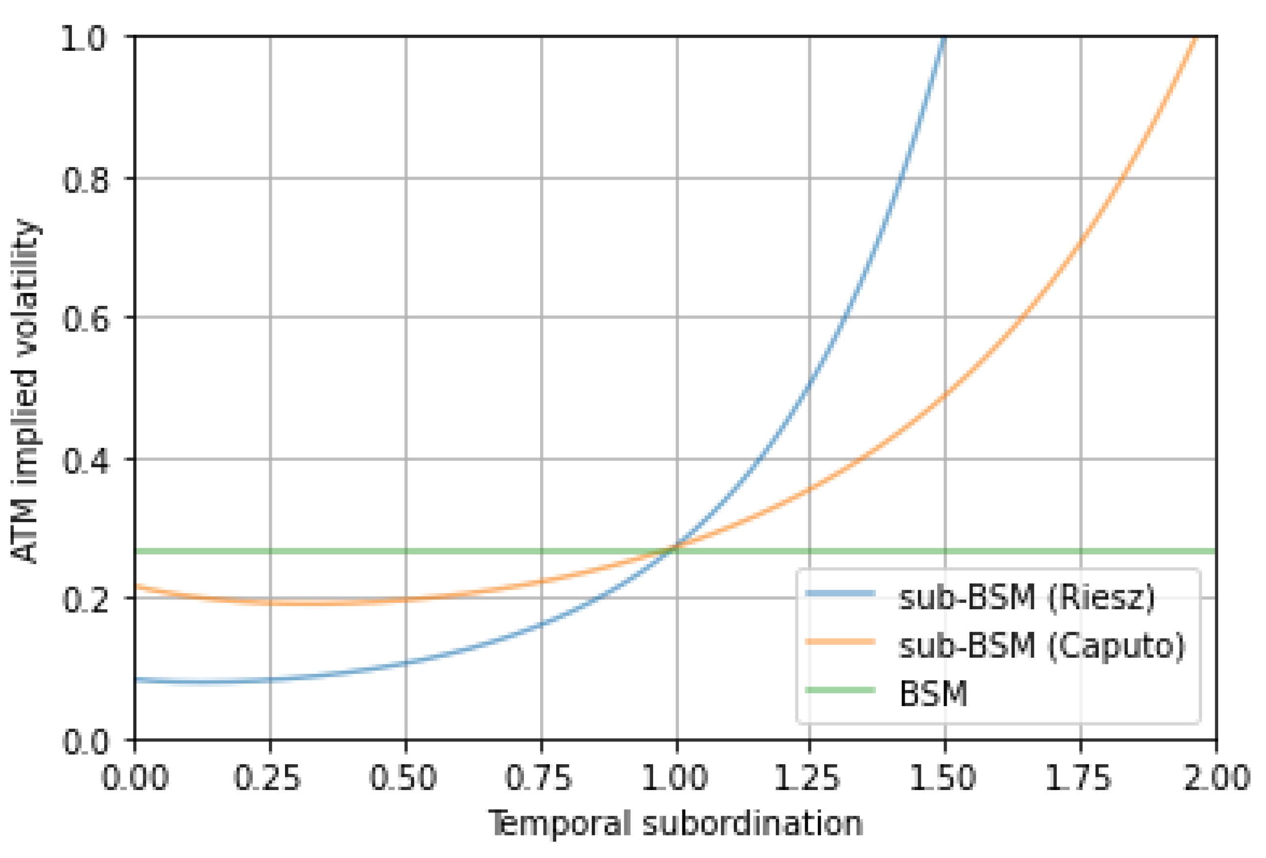
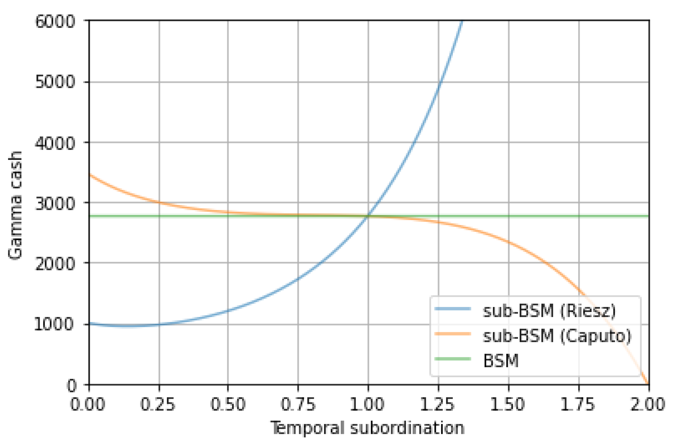
Taking $\alpha =2$ defines a “subordinated Black–Scholes model” sub-BSM$(\gamma )$, in the sense that there is no fat tail but a subordination parameter induced by the order of the Riesz time derivative. A similar model had already been introduced in [48] but in the case of a Caputo time derivative.

-

Taking $\alpha =2$ and $\gamma =1$ recovers the usual Black–Scholes–Merton model BSM$(\sigma \sqrt{2})$ [2]. In that case. the process is purely Gaussian, there is no fat tail nor temporal subordination and the RFFD Equation (29) degenerates into the usual heat Equation (8).

-

Let us also mention that the case $\alpha =\gamma$ (or equivalently $\Omega =1$) corresponds to the so-called neutral diffusion, but is only of limited financial interest.

Remark 4.

In principle, it is possible to extend the FPDE (29) to more than one dimension. In a financial context, it corresponds to options written on several assets, such as spread options for instance (interestingly, no closed pricing formula exist for such instruments in general, even in the basic BSM$(\sigma )$ model). However, in the case of a process with more than one spatial dimension, the set of parameters $(\alpha ,\theta ,\gamma )$ that preserve positivity of the solution is more complicated (see e.g., [62]) and we would have to divide the results into two separate cases, i.e., for one-dimensional space and for more-dimensional space.

4.3. Convexity Adjutment

Before deriving a formula for $\omega$ in terms of a Mellin–Barnes integral and expressing it as a sum of residues, let us recall that the Green function of the RFFD$(\alpha ,\gamma )$ model can be separated as an integral composition of two kernels (see e.g., [31]):

$$g_{\alpha ,\gamma }(x,\tau )=\frac{\Gamma (\gamma )}{{\tau }^{\gamma }}\underset{0}{\overset{\infty }{\int }}{g}_{\gamma }(t,y)g_{\alpha }(x,y)dy.$$

(34)

By using the relation (A12) in Appendix B.2 we can write:

$$g_{\alpha ,\gamma }(x,\tau )=\frac{\Gamma (\gamma +1)}{{\tau }^{2\gamma }}\underset{0}{\overset{\infty }{\int }}y{M}_{\gamma }\left(\frac{y}{{\tau }^{\gamma }}\right)g_{\alpha }(y,x)dy,$$

(35)

where $M_{\nu }(z)$ denotes the Wright M-function.

Proposition 1.

The convexity adujstment ω of the RFFD$(\alpha ,\gamma )$ model can be written as:

$$\omega =-log\left[\frac{\Gamma (\gamma +1)}{\alpha }\underset{c-i\infty }{\overset{c+i\infty }{\int }}\frac{\Gamma (s)\Gamma (\frac{2-s}{\alpha })}{\Gamma (\gamma s-\gamma +1)}{\omega }_{\alpha }^{\frac{s-2}{\alpha }}\frac{ds}{2i\pi }\right]$$

(36)

where ${\omega }_{\alpha }$ is the FMLS$(\alpha )$ convexity adjustment (24), and where $c\in (0,2)$.

Proof. 

By inserting the composition rule (35) into the definition of the convexity adjustment (33) and switching the order of integration, we have:

$$\omega =-log\left[\Gamma (\gamma +1)\underset{0}{\overset{\infty }{\int }}y{M}_{\gamma }(y)\underset{-\infty }{\overset{\infty }{\int }}{e}^x{g}_{\alpha }(x,y)dxdy\right].$$

(37)

The x-integral is nothing else than the bilateral Laplace transform of the asymmetric stable distribution and, as such, equals (see Equation (23)) $e^{-{\omega }_{\alpha }{y}^{\alpha }}$. Introducing the Mellin–Barnes representation (A11) for the Wright M-function, we obtain:

$$\omega =-log\left[\Gamma (\gamma +1)\underset{c-i\infty }{\overset{c+i\infty }{\int }}\frac{\Gamma (s)}{\Gamma (\gamma s-\gamma +1)}\underset{0}{\overset{\infty }{\int }}{y}^{1-s}{e}^{-{\omega }_{\alpha }{y}^{\alpha }}dy\frac{ds}{2i\pi }\right]$$

(38)

for $c>0$. Performing the y integral, which converges for $Re(s)<2$, yields (36). □

Corollary 1.

The convexity adjustment ω of the RFFD$(\alpha ,\gamma )$ model can be written as:

$$\omega =-log\left[\Gamma (\gamma +1)\sum _{n=0}^{\infty }\frac{\Gamma (\alpha n+2)}{\Gamma (\alpha \gamma n+\gamma +1)}\frac{{(-{\omega }_{\alpha })}^n}{n!}\right].$$

(39)

Proof. 

Consider a contour closing the vertical line of integration in (36) right of the line $Re(s)=2$; in this half plane there is a series of simple poles induced by the analytic continuation of the $\Gamma (\frac{2-s}{\alpha })$ function, occurring at $s=\alpha n+2$, $n\in \mathbb{N}$. From the singular behavior of the Gamma function (see Appendix B.1), the residues are:

$$Res\left[\frac{\Gamma (s)\Gamma (\frac{2-s}{\alpha })}{\Gamma (\gamma s-\gamma +1)}{\omega }_{\alpha }^{\frac{s-2}{\alpha }},s=\alpha n+2\right]=\alpha \frac{{(-1)}^n}{n!}\frac{\Gamma (\alpha n+2)}{\Gamma (\alpha \gamma n-\gamma +1)}{\omega }_{\alpha }^n.$$

(40)

Summing all residues and simplifying yields (39). □

Remark 5.

Let us remark some interesting particular cases of (39):

-

If one takes $\gamma =1$ in (39) then:

$$\omega =-log\left[\sum _{n=0}^{\infty }\frac{{(-{\omega }_{\alpha })}^n}{n!}\right]=-log{e}^{-{\omega }_{\alpha }}={\omega }_{\alpha }$$

(41)

and one recovers the FMLS convexity adjustment in this case;

-

Using the usual Taylor expansion for $log(1+u)$, we can write:

$$\omega =\frac{\Gamma (\gamma +1)\Gamma (\alpha +2)}{\Gamma (\alpha \gamma +\gamma +1)}{\omega }_{\alpha }+O\left({\omega }_{\alpha }^2\right).$$

(42)

-

Taking $\alpha =2$ in (42) yields, at first order,

$$\omega =\frac{6\Gamma (\gamma +1)}{\Gamma (3\gamma +1)}{\omega }_2$$

(43)

and when furthermore $\gamma =1$ we are left with $\omega =-{\sigma }^2$ which is the usual adjustment in the BSM$(\sigma \sqrt{2})$ model.

4.4. Pricing Formula in the Mellin Space

Let us introduce the function:

$$g_{\alpha ,\gamma }^{*}(s_1)=\frac{\Gamma (1-s_1)}{\Gamma (\gamma -\frac{\gamma }{\alpha }{s}_1)}$$

(44)

which exists and is analytic in the whole half-plane $\{Re(s_1)<1\}$. Let us also assume that the payoff function is supported by the real positive axis only, that is:

$$\mathrm{supp}\left(x\to \mathcal{P}(S(t)e^{(r-q+\omega )\tau +x})\right)\subset {\mathbb{R}}_{+},$$

(45)

and denote its Mellin transform by:

$$p^{*}(s_1)=\underset{0}{\overset{\infty }{\int }}\mathcal{P}(S(t)e^{(r-q+\omega )\tau +x})x^{s_1-1}dx$$

(46)

which is assumed to converge in a domain of $\mathbb{C}$ of the form $\{a_{-}<Re(s_1)<a_{+}\}$. Then, as a consequence of the pricing formula (32) we have the following proposition:

Proposition 2

(Pricing formula). In the RFFD$(\alpha ,\gamma )$ model, the price at time t of a contingent claim delivering a payoff $\mathcal{P}(S_T)$ at its maturity T can be written as:

$$\mathcal{C}(t)=e^{-r\tau }\frac{\Gamma (\gamma )}{\alpha }\underset{c-i\infty }{\overset{c+i\infty }{\int }}{g}_{\alpha ,\gamma }^{*}(s_1)p^{*}(s_1){\left(-\omega {\tau }^{\gamma }\right)}^{-\frac{s_1}{\alpha }}\frac{d{s}_1}{2i\pi }$$

(47)

for any $c\in (a_{-},a_{+})\cap (-\infty ,1)$, and where the intersection is assumed to be nonempty.

Remark 6.

Extension to negatively supported payoff functions is straightforward, via the symmetry relation (31).

5. Application to Vanilla and Exotic Path Independent Options

In this section we apply Proposition 2 to several commonly traded options.

5.1. Digital

Digital options are either asset or nothing (a/n) or cash or nothing (c/n); in this subsection we only discuss the a/n option, as the c/n option price will be obtained as a corollary in the next subsection.

An a/n call pays one unit of the underlying stock $S(T)$ at maturity, on the condition that it ends up higher that some pre-determined strike price K. We can write the payoff as:

$${\mathcal{P}}_{a/n}(S(T))=S(T){\mathbb{1}}_{(K,+\infty )}(S(T)).$$

(48)

Remark 7.

Introducing the (log forward) moneyness:

$$k=log\frac{S(t)}{K}+(r-q+\omega )\tau$$

(49)

allows us to write:

$${\mathcal{P}}_{a/n}\left(S(t)e^{(r-q+\omega )\tau +x}\right)=K{e}^{k+x}{\mathbb{1}}_{(-k,+\infty )}(x),$$

(50)

and therefore the positive support condition (45) is equivalent to the condition $k<0$. Options satisfying this condition are said to be Out of the Money (OTM), while options with $k>0$ are said to be in the money (ITM). $k=0$ corresponds to the at the money (ATM) situation. We will only detail the proof in the OTM case, because the extension to the ITM case can be made thanks to the symmetry relation (31) and with the same result than in the OTM case.

Proposition 3.

In the RFFD$(\alpha ,\gamma )$ model, the value at time t of an asset or nothing call option is:

$${\mathcal{C}}_{a/n}(t)=\frac{K{e}^{-r\tau }\Gamma (\gamma )}{\alpha }\sum _{n_1,n_2=0}^{\infty }\frac{k^{n_1}}{n_1!\Gamma (\gamma +\gamma \frac{-n_1+n_2}{\alpha })}{(-\omega {\tau }^{\gamma })}^{\frac{-n_1+n_2}{\alpha }}.$$

(51)

Proof. 

Using (50) and a Mellin–Barnes representation for the exponential term (see (A8) in Appendix B.1), we can write the Mellin transform (46) as:

$$p^{*}(s_1)=K\underset{c_2-i\infty }{\overset{c_2+i\infty }{\int }}{(-1)}^{-s_2}\Gamma (s_2)\underset{-k}{\overset{\infty }{\int }}{(k+x)}^{-s_2}{x}^{s_1-s_2-1}dx\frac{d{s}_2}{2i\pi }.$$

(52)

Assuming $k<0$, performing the x-integral and using proposition 2, we get the asset or nothing price:

$$\begin{array}{c}{\mathcal{C}}_{a/n}(t)=K{e}^{-r\tau }\frac{\Gamma (\gamma )}{\alpha }\times \hfill \\ \hfill \underset{c_1-i\infty }{\overset{c_1+i\infty }{\int }}\underset{c_2-i\infty }{\overset{c_2+i\infty }{\int }}{(-1)}^{-s_2}\frac{\Gamma (s_2)\Gamma (1-s_2)\Gamma (-s_1+s_2)}{\Gamma (\gamma -\frac{\gamma }{\alpha }{s}_1)}{(-k)}^{s_1-s_2}{(-\omega {\tau }^{\gamma })}^{-\frac{s_1}{\alpha }}\frac{d{s}_{1}d{s}_2}{{(2i\pi )}^2}\end{array}$$

(53)

which is analytic in the polyhedron:

$$\left\{(s_1,s_2)\in {\mathbb{C}}^2,0<Re(s_2)<1,Re(-s_1+s_2)>0\right\}\subset {\mathbb{C}}^2.$$

(54)

Outside this polyhedron, we know from the singular behavior of the gamma function around negative integers (see Appendix B.1) that the integrand has poles when $(s_1,s_2)=(n_1-n_2,-n_2)$, $n_1,n_2\in \mathbb{N}$, and by summing the associated residues, we obtain:

$$\begin{array}{c}{\mathcal{C}}_{a/n}(t)=K{e}^{-r\tau }\frac{\Gamma (\gamma )}{\alpha }\times \hfill \\ \hfill \sum _{n_1,n_2=0}^{\infty }{(-1)}^{n_2}\frac{{(-1)}^{n_1+n_2}}{n_1!n_2!}\frac{\Gamma (1+n_2)}{\Gamma (\gamma -\frac{\gamma }{\alpha }(n_1-n_2))}{(-k)}^{n_1}{(-\omega {\tau }^{\gamma })}^{\frac{-n_1+n_2}{\alpha }}.\end{array}$$

(55)

Simplifying (recall that $\Gamma (1+n_2)=n_2!$) completes the proof. □

5.2. European

One of the most traded option contracts is the so-called European option, which pays the difference between the maturity price $S(T)$ and the strike price K, on the condition that the difference is positive. The payoff can therefore be written as:

$${\mathcal{P}}_{eur}(S(T))=(S(T)-K){\mathbb{1}}_{(K,+\infty )}(S(T))={\left[S(T)-K\right]}^{+}.$$

(56)

Similarly to (50), we can write:

$${\mathcal{P}}_{eur}\left(S(t)e^{(r-q+\omega )\tau +x}\right)=K(e^{k+x}-1){\mathbb{1}}_{(-k,+\infty )}(x),$$

(57)

and, using the Mellin–Barnes representation (A9) for the $e^{k+x}-1$ term and proceeding exactly like in the proof of Proposition 3, we obtain:

Proposition 4.

In the RFFD$(\alpha ,\gamma )$ model, the value at time t of a European call option is:

$${\mathcal{C}}_{eur}(t)=\frac{K{e}^{-r\tau }\Gamma (\gamma )}{\alpha }\sum _{\begin{array}{c}{n}_1=0\\ n_2=1\end{array}}^{\infty }\frac{k^{n_1}}{n_1!\Gamma (\gamma +\gamma \frac{-n_1+n_2}{\alpha })}{(-\omega {\tau }^{\gamma })}^{\frac{-n_1+n_2}{\alpha }}.$$

(58)

Remark 8.

Observe that the only difference between the pricing formulas for the a/n calls and the European call lies in the summation index $n_2$, which starts at 0 in the a/n case and at 1 in the European case. This is a direct consequence of the contour deformation between representations (A8) and (A9), which modifies the polyhedron of analyticity (54) accordingly.

Let us also introduce the cash or nothing (c/n) call option (which is also itself a digital option); this option pays a constant amount (say 1) if and if only the terminal price ends up above the strike:

$${\mathcal{P}}_{c/n}(S(T))={\mathbb{1}}_{(K,+\infty )}(S(T)).$$

(59)

We can notice that the c/n call is a linear combination of a/n and European call options, namely:

$${\mathcal{P}}_{c/n}(S(T))=\frac{1}{K}\left({\mathcal{P}}_{a/n}(S(T))-{\mathcal{P}}_{eur}(S(T)\right),$$

(60)

and, from Propositions 3 and 4, we obtain:

Corollary 2.

In the RFFD$(\alpha ,\gamma )$ model, the value at time t of a cash or nothing call option is:

$${\mathcal{C}}_{c/n}(t)=\frac{e^{-r\tau }\Gamma (\gamma )}{\alpha }\sum _{n_1=0}^{\infty }\frac{k^{n_1}}{n_1!\Gamma (\gamma -\gamma \frac{n_1}{\alpha })}{(-\omega {\tau }^{\gamma })}^{\frac{-n_1}{\alpha }}.$$

(61)

5.3. Power

A power option is a non-linear version of the European call, which delivers the payoff:

$${\mathcal{P}}_{pow}(S(T))={\left[S{(T)}^a-K\right]}^{+}.$$

(62)

for some positive number a. We can therefore write:

$${\mathcal{P}}_{pow}\left(S(t)e^{(r-q+\omega )\tau +x}\right)=K(e^{a(k_a+x)}-1){\mathbb{1}}_{(-k_a,+\infty )}(x),$$

(63)

where we have introduced the modified moneyness:

$$k_a=log\frac{S(t)}{K^{\frac{1}{a}}}+(r-q+\omega )\tau$$

(64)

which coincides with the usual moneyness k when $a=1$. Proceeding like for the European option, we immediately obtain:

Proposition 5.

In the RFFD$(\alpha ,\gamma )$ model, the value at time t of a power call option is:

$${\mathcal{C}}_{pow}(t)=\frac{K{e}^{-r\tau }\Gamma (\gamma )}{\alpha }\sum _{\begin{array}{c}{n}_1=0\\ n_2=1\end{array}}^{\infty }\frac{a^{n_2}{k}_a^{n_1}}{n_1!\Gamma (\gamma +\gamma \frac{-n_1+n_2}{\alpha })}{(-\omega {\tau }^{\gamma })}^{\frac{-n_1+n_2}{\alpha }}.$$

(65)

5.4. Log

Log options (see [34]) are options written directly on the stock’s log returns:

$${[logS(T)-logK]}^{+}.$$

(66)

Let us also mention that the log put option pays ${\mathcal{P}}_{logput}(S(T)):={[logK-logS(T)]}^{+}$ and that the log contract is obtained by being long of a log call and short of a log put; a delta hedged log contract is called a variance swap.

Proposition 6.

In the RFFD$(\alpha ,\gamma )$ model, the value at time t of a log call option is:

$$C_{log}=\frac{e^{-r\tau }\Gamma (\gamma )}{\alpha }\sum _{n=0}^{\infty }\frac{k^n}{n!\Gamma \left(\gamma +\gamma \frac{1-n}{\alpha }\right)}{(-\omega {\tau }^{\gamma })}^{\frac{1-n}{\alpha }}.$$

(67)

Proof. 

Let us note that:

$${\mathcal{P}}_{log}\left(S(t)e^{(r-q+\omega )\tau +x}\right)={[k+x]}^{+}$$

(68)

therefore, the Mellin transform (46) for the payoff function can be computed directly:

$$p^{*}(s_1)=\underset{-k}{\overset{\infty }{\int }}(k+x)x^{s_1-1}dx=\frac{{(-k)}^{1+s_1}}{s_1(1+s_1)}.$$

(69)

Using Proposition 2 and the functional relation $\Gamma (1-s_1)=-s_1\Gamma (-s_1)$, the option price is:

$${\mathcal{C}}_{log}(t)=\frac{e^{-r\tau }\Gamma (\gamma )}{\alpha }\underset{c_1-i\infty }{\overset{c_1+i\infty }{\int }}-\frac{\Gamma (-s_1)}{(1+s_1)\Gamma (\gamma -\gamma \frac{s_1}{\alpha })}{(-k)}^{1+s_1}{(-\omega {\tau }^{\gamma })}^{-\frac{s_1}{\alpha }}\frac{d{s}_1}{2i\pi }$$

(70)

which converges for $Re(s_1)<-1$. The analytic continuation of the integrand in the right half-plane has:

-

A simple pole in $s_1=-1$ with residue:

$$\frac{{(-\omega {\tau }^{\gamma })}^{\frac{1}{\alpha }}}{\Gamma (\gamma +\frac{\gamma }{\alpha })},$$

(71)

-

A series of poles at every positive integer $s_1=n$ with residues:

$$-\frac{{(-1)}^n}{(n+1)!}\frac{1}{\Gamma (\gamma -\gamma \frac{n}{\alpha })}{(-k)}^{1+n}{(-\omega {\tau }^{\gamma })}^{-\frac{n}{\alpha }}.$$

(72)

Summing the residues (71) and (72) for all n and re-ordering yields the announced result. □

6. Impact on Volatility Modeling and Hedging Policies

Let us now discuss some interesting features of the RFFD$(\alpha ,\gamma )$ model in terms of volatility modeling, delta hedging, and profit and loss calculation, and compare with another time fractional model and with the classical Black–Scholes–Merton model.

6.1. At the Money Forward Price and Volatility

An interesting situation occurs when stock price is at the money forward (ATMF), that is when $S(t)=\overline{S}(t)$ where:

$$\overline{S}(t)=K{e}^{-r\tau }.$$

(73)

Taking only the leading term $(n_1=0,n_2=1)$ in the European price series (Proposition 4), we can approximate the ATMF call price by:

$${\overline{\mathcal{C}}}_{eur}(t)=\frac{\overline{S}(t)}{\alpha }\frac{\Gamma (\gamma )}{\Gamma (\gamma +\frac{\gamma }{\alpha })}{\left(-\omega {\tau }^{\gamma }\right)}^{\frac{1}{\alpha }}.$$

(74)

Taking $\alpha =2$ (sub-BSM$(\gamma )$ model) and using the approximation (43) for the convexity adjustment, we obtain:

$${\overline{\mathcal{C}}}_{eur}(t)=\overline{S}(t)\frac{\Gamma (\gamma )}{\Gamma (\frac{3\gamma }{2})}{\left(\frac{3\Gamma (\gamma +1)}{2\Gamma (3\gamma +1)}{\tau }^{\gamma }\right)}^{\frac{1}{2}}\sigma$$

(75)

and, therefore, we have a compact formula for the ATMF implied volatility:

$$\overline{\sigma }=\frac{{\overline{\mathcal{C}}}_{eur}(t)}{\overline{S}(t)}\frac{\Gamma (\frac{3\gamma }{2})}{\Gamma (\gamma )}{\left(\frac{3\Gamma (\gamma +1)}{2\Gamma (3\gamma +1)}{\tau }^{\gamma }\right)}^{-\frac{1}{2}}.$$

(76)

Letting $\gamma \to 1$ in (76) we recover the formula for the ATMF implied volatility in the Black–Scholes–Merton BSM$(\sigma \sqrt{2})$ model (recall that $\Gamma (3/2)=\sqrt{\pi }/2$):

$${\overline{\sigma }}_{BSM}=\frac{{\overline{\mathcal{C}}}_{eur}(t)}{\overline{S}(t)}\sqrt{\frac{\pi }{\tau }}.$$

(77)

Remark 9.

A similar implied volatility formula was derived in [63] in the case where the time fractional derivative is of a Caputo type, instead of a Riesz type, and reads:

$${\overline{\sigma }}_C=\frac{{\overline{\mathcal{C}}}_{eur}(t)}{\overline{S}(t)}\Gamma \left(1+\frac{\gamma }{2}\right){\left(\frac{{\tau }^{\gamma }}{2\Gamma (2\gamma +1)}\right)}^{-\frac{1}{2}}.$$

(78)

In Figure 1 we plot the implied volatility in the sub-BSM$(\gamma )$ model, either with a Riesz temporal derivative (Equation (76) or a Caputo temporel derivative (Equation (78)), and the BSM implied volatility (Equation (77)), for $\gamma \in (0,2)$. We can observe the sharper volatility behavior in the Riesz case, with a lower implied volatility than in the Caputo case in the slow diffusion regime ($\gamma <1$), but a higher one in the fast diffusion regime ($\gamma >1$). Of course all models lead to the same implied volatility in the non-fractional regime ($\gamma =1$).

6.2. Delta Hedging

The derivative of an option with respect to the underlying stock price is generally denoted by $\Delta$ (Delta). It is a crucial measure for portfolio management as it quantifies the sensitivity of the contract to underlying market moves. Deriving Proposition 4 with respect to $S(t)$ and re-arranging the terms, it is straightforward to obtain the Delta of the European call in the RFFD$(\alpha ,\gamma )$ model:

$$\Delta =\frac{K{e}^{-r\tau }}{S(t)}\frac{\Gamma (\gamma )}{\alpha }\sum _{n_1,n_2=0}^{\infty }\frac{k^{n_1}}{n_1!\Gamma (\gamma +\gamma \frac{-n_1+n_2}{\alpha })}{(-\omega {\tau }^{\gamma })}^{\frac{-n_1+n_2}{\alpha }}.$$

(79)

In the ATMF situation ($S(t)=K{e}^{-r\tau }$), we have, at first order:

$$\Delta =\frac{\Gamma (\gamma )}{\alpha }\times \frac{1}{\Gamma (\gamma )}=\frac{1}{\alpha }.$$

(80)

Equation (80) is remarkable because it shows that the order of the time-fractional derivative $\gamma$ plays no role (at least at first order) in the value of the option’s delta, which is entirely governed by the tail parameter $\alpha$. In other words, it suffices to be the long (buyer) of one unit of the stock $S(t)$ and short (seller) of $\alpha$ units of an option $\mathcal{C}(t)$ to protect the portfolio against market moves, whatever the subordination parameter $\gamma$. Remarkably too, a similar behavior had been noted in the case of a temporal Caputo derivative in [63], and is therefore preserved in the case of a Riesz derivative. This behavior is summarized in

Table 1. The RFFD$(\alpha ,\gamma )$ model: Impacts of the fractional parameters.

	Space Derivative $\mathit{\alpha }$	Time Derivative $\mathit{\gamma }$
Randomness	Yes: Wild randomness if $\alpha \in (1,2)$ Mild randomness if $\alpha =2$	No
Regime	No	Yes: Slow diffusion if $\gamma <1$ Fast diffusion if $\gamma \ge 1$
ATM prices/volatility	Yes	Yes
Delta hedging	Yes: Long 1 stock $S(t)$ Short α call options ${\mathcal{C}}_{eur}(t)$	No
Delta hedged P&L	Yes	Yes

, alongside the impacts of the parameters on implied volatility, profit, and loss (see following subsection) and on the model’s randomness and regimes.

6.3. Profit and Loss

Similarly to the Delta, we define the $\Gamma$ (Gamma) of an option as the second derivative of the option’s price with respect to the stock price $S(t)$. The market profit and loss (P& L) between two trading days $t_1$ and $t_2$ can therefore be written as:

$$\mathrm{market}\mathrm{P}\&\mathrm{L}=\Delta (\Delta S_t)+\frac{1}{2}\Gamma {(\Delta S(t))}^2,\Delta S(t):=S(t_2)-S(t_1).$$

(81)

Assuming that the portfolio has been delta-hedged, we are left with:

$$\mathrm{market}\mathrm{P}\&\mathrm{L}=\$\Gamma {\left(\frac{\Delta S(t)}{S(t)}\right)}^2$$

(82)

where the Dollar Gamma, or Gamma cash, has been defined by $\$\Gamma :=\frac{1}{2}S{(t)}^2\Gamma$; relation (82) is very popular in portfolio management, because it allows to express the returns of a portfolio in terms of the realized variance of the underlying returns. By deriving (79) with respect to $S(t)$, we obtain the Gamma of the European call:

$$\Gamma =\frac{K{e}^{-r\tau }}{S{(t)}^2}\frac{\Gamma (\gamma )}{\alpha }\sum _{n_1=0}^{\infty }\frac{k^n}{n!\Gamma (\gamma -\frac{\gamma }{\alpha }(n_1+1))}{(-\omega {\tau }^{\gamma })}^{-\frac{n+1}{\alpha }}$$

(83)

which, remarkably, can be represented as a sum over one index only (because of the simplification of all terms for $n_2>0$ when differentiating the series (79)).

In the ATMF situation and if $\alpha =2$, using the approximation (43) for the convexity adjustment and usual formulas (Legendre duplication) for the Gamma function, we get:

$$\Gamma =\frac{2^{\gamma -2}}{\sqrt{\pi }\overline{S}(t)\sigma }\Gamma \left(\frac{\gamma +1}{2}\right){\left(\frac{6\Gamma (\gamma +1)}{\Gamma (3\gamma +1)}{\tau }^{\gamma }\right)}^{-\frac{1}{2}}$$

(84)

and the Gamma cash:

$$\$\Gamma =\frac{2^{\gamma -3}}{\sqrt{\pi }\sigma }\overline{S}(t)\Gamma \left(\frac{\gamma +1}{2}\right){\left(\frac{6\Gamma (\gamma +1)}{\Gamma (3\gamma +1)}{\tau }^{\gamma }\right)}^{-\frac{1}{2}}.$$

(85)

Note that, as expected,

$$\$\Gamma \stackrel{\gamma \to 1}{⟶}\frac{\overline{S}(t)}{4\sigma \sqrt{\pi \tau }}$$

(86)

thus recovering the usual Gamma cash is the BSM$(\sigma \sqrt{2})$ model.

Remark 10.

In the case of a Caputo time derivative, a formula has also been derived for the Gamma in [63] and reads in that case:

$$\${\Gamma }_C=\frac{\overline{S}(t)}{4\sigma \sqrt{2}}\frac{\sqrt{\Gamma (1+2\gamma )}}{\Gamma (1-\frac{\gamma }{2})}\frac{1}{{\tau }^{\frac{\gamma }{2}}}.$$

(87)

InFigure 2, we compare the behavior of the Gamma cash in the case of a Riesz time derivative, Caputo time derivative and non-fractional BSM$(\sigma \sqrt{2})$ model. Again, all models coincide for $\gamma =1$, but the behavior of the two subordinated models is very different, Gamma cash (and, therefore, market P&L) being either an increasing or a decreasing function of the subordination parameter γ. Note that the characteristic shape of the Gamma cash in the Caputo case, with its inflexion at $\gamma =1$, had already been noted in [47].

In Table 1 we summarize the observations we made in this section on volatility modeling, delta hedging policy, and Gamma cash (P&L), as well as the impact of the order of fractional derivatives of the model’s randomness and regimes as defined in Section 3 and Section 4.

7. Conclusions

In this paper, we proposed a review of the market models linked to space-fractional derivatives and showed how the order of these derivatives could be interpreted as a measure of randomness of the model. Moreover, the fractional formulation also allows for a natural extension in terms of time-fractional derivatives, whose order is interpreted as a subordination parameter controlling the temporal redistribution of risk across maturities, for instance.

We were also able to define the fundamental concepts of option pricing in the framework of a model-driven by the space-time fractional diffusion, and we applied this setup to the case of a Riesz temporal derivative. Although this model was introduced earlier in the literature, no analytical tools had been derived for option pricing and hedging so far; in the present work, we have therefore established closed-form formulas for the price of several options (European, digital, power, and log) and of the model’s convexity adjustment. As these formulas are simple sums of powers of the model’s parameters (such as moneyness and convexity adjustment), they do not call for sophisticated numerical tools to be estimated in practice. We have also studied the impact of the order of both space- and time-fractional derivatives on implied volatility, delta hedging, and profit and loss; maybe the most interesting result is that the delta hedging policy was shown not to be affected by the time-fractional derivative but governed by the space derivative only, while profit and loss are affected by both parameters. A similar behavior had been noted in the previously studied fractional diffusion models that involved a Caputo derivative. The shape of the profit and loss function is, however, very different between the two models.

Future works should include the extension to other types of options or fractional derivatives. We would also like to apply the space-time fractional diffusion approach to other fields of quantitative finance, such as default modeling.

References

1. Bachelier, L. Théorie de la spéculation. Ann. Sci. Éc. Norm. Supér. 1900, 3, 21–86. [Google Scholar] [CrossRef]
2. Black, F.; Scholes, M. The Pricing of Options and Corporate Liabilities. J. Polit. Econ. 1973, 81, 637–654. [Google Scholar] [CrossRef] [Green Version]
3. Merton, R. Theory of Rational Option Pricing. Bell J. Econ. Manag. Sci. 1973, 4, 141–183. [Google Scholar] [CrossRef] [Green Version]
4. Heston, S.L. A Closed-Form Solution for Options with Stochastic Volatility with Applications to Bond and Currency Options. Rev. Financ. Stud. 1993, 6, 327–343. [Google Scholar] [CrossRef] [Green Version]
5. Cont, R.; Tankov, P. Financial Modelling with Jump Processes; Chapman & Hall: New York, NY, USA, 2004. [Google Scholar]
6. Krawiecki, A.; Holyst, J.A.; Helbing, D. Volatility Clustering and Scaling for Financial Time Series due to Attractor Bubbling. Phys. Rev. Lett. 2000, 89, 158701. [Google Scholar] [CrossRef] [Green Version]
7. Mandelbrot, B. Fractals and Scaling in Finance: Discontinuity, Concentration, Risk; Springer: New York, NY, USA, 1997. [Google Scholar]
8. Calvet, L.; Fischer, A. Multifractal Volatility: Theory, Forecasting, and Pricing; Academic Press: Cambridge, UK, 2008. [Google Scholar]
9. Chatterjee, A.; Yarlagadda, S.; Chakrabarti, B.K. Econophysics of Wealth Distributions; Springer: Milan, Italy, 2005. [Google Scholar]
10. D’Arcangelis, A.M.; Rotundo, G. Complex networds in finance. In Complex Networks and Dynamics. Lecture Notes in Economics and Mathematical Systems; Commendatore, P., Matilla-García, M., Varela, L., Cánovas, J., Eds.; Springer: Cham, Switzerland, 2016; Volume 683. [Google Scholar]
11. Mantegna, R.N.; Stanley, H.E. An Introduction to Econophysics: Correlations and Complexity in Finance; Cambridge University Press: Cambridge, UK, 1999. [Google Scholar]
12. Mantegna, R.N.; Stanley, H.E. Stochastic process with ultraslow convergence to a Gaussian: The truncated Lévy flight. Phys. Rev. Lett. 1994, 73, 2946. [Google Scholar] [CrossRef]
13. Koponen, E. Analytic approach to the problem of convergence of truncated Lévy flights towards the Gaussian stochastic process. Phys. Rev. E 1995, 52, 1197–1199. [Google Scholar] [CrossRef]
14. Carr, P.; Geman, H.; Madan, D.; Yor, M. The Fine Structure of Asset Returns: An Empirical Investigation. J. Bus. 2002, 75, 305–332. [Google Scholar] [CrossRef] [Green Version]
15. Boyarchenko, S.; Levendorskii, S. Non Gaussian Black-Scholes-Merton Theory; World Scientific Publishing Co.: River Edge, NJ, USA, 2002. [Google Scholar]
16. Rosinski, J. Tempering Stable Processes. Stoch. Process. Their Appl. 2007, 117, 677–707. [Google Scholar] [CrossRef] [Green Version]
17. Madan, D.; Carr, P.; Chang, E. The Variance Gamma Process and Option Pricing. Eur. Financ. Rev. 1998, 2, 79–105. [Google Scholar] [CrossRef] [Green Version]
18. Podlubny, I. Fractional Differential Equations; Academic Press: San Diego, CA, USA, 1999. [Google Scholar]
19. Samko, S.G.; Kilbas, A.A.; Marichev, O.I. Fractional Integrals and Derivatives: Theory and Applications; Gordon and Breach: New York, NY, USA, 1993. [Google Scholar]
20. Kochubei, A.; Luchko, Y. (Eds.) Handbook of Fractional Calculus with Applications. Volume 1: Basic Theory; De Gruyter: Berlin, Germany, 2019. [Google Scholar]
21. Kochubei, A.; Luchko, Y. (Eds.) Handbook of Fractional Calculus with Applications. Volume 2: Fractional Differential Equations; De Gruyter: Berlin, Germany, 2019. [Google Scholar]
22. Cartea, A.; Del-Castillo-Negrete, D. Fractional diffusion models of option prices in markets with jumps. Physica A 2007, 374, 749–763. [Google Scholar] [CrossRef] [Green Version]
23. Carr, P.; Wu, L. The Finite Moment Log Stable Process and Option Pricing. J. Financ. 2003, 58, 753–777. [Google Scholar] [CrossRef] [Green Version]
24. Feller, W. An Introduction to Probability Theory and Its Applications, 2nd ed.; John Wiley & Sons: New York, NY, USA, 1971; Volume II. [Google Scholar]
25. Gorenflo, R.; Mainardi, F. Random walk models for space-fractional diffusion processes. Fract. Calc. Appl. Anal. 1998, 1, 167–191. [Google Scholar]
26. Carte, A. Derivatives pricing with marked point processes using tick-by-tick data. Quant. Financ. 2013, 13, 111–123. [Google Scholar] [CrossRef] [Green Version]
27. Clark, P. A subordinated stochastic process model with fixed variance for speculative prices. Econometrica 1973, 41, 135–155. [Google Scholar] [CrossRef]
28. Carr, P.; Wu, L. Time-changed Lévy processes and option pricing. J. Financ. Econ. 2004, 71, 113–141. [Google Scholar] [CrossRef] [Green Version]
29. Gorenflo, R.; Mainardi, F.; Vivoli, A. Discrete and Continuous Random Walk Models for Space-Time Fractional Diffusion. J. Math. Sci. 2006, 132, 614–628. [Google Scholar] [CrossRef]
30. Korbel, J.; Luchko, Y. Modeling of financial processes with a space-time fractional diffusion equation of varying order. Fract. Calc. Appl. Anal. 2016, 19, 1414–1433. [Google Scholar] [CrossRef]
31. Kleinert, H.; Korbel, J. Option Pricing Beyond Black-Scholes Based on Double-Fractional Diffusion. Physica A 2016, 449, 200–214. [Google Scholar] [CrossRef] [Green Version]
32. Tarasov, V.E.; Tarasova, V.V. Macroeconomic models with long dynamic memory: Fractional calculus approach. Appl. Math. Comput. 2018, 338, 466–486. [Google Scholar] [CrossRef]
33. Tomovski, Z.; Dubbeldam, J.L.A.; Korbel, J. Applications of Hilfer-Prabhakar operator to option pricing financial model. Fract. Calc. Appl. Anal. 2020, 23, 996–1012. [Google Scholar] [CrossRef]
34. Wilmott, P. Paul Wilmott on Quantitative Finance; Wiley & Sons: Hoboken, NJ, USA, 2006. [Google Scholar]
35. Carr, P.; Madan, D. Option valuation using the Fast Fourier Transform. J. Comput. Financ. 1999, 2, 61–73. [Google Scholar] [CrossRef] [Green Version]
36. Lewis, A. A Simple Option Formula for General Jump-Diffusion and Other Exponential Lévy Processes. SSRN 2001, SSRN 282110. Available online: https://ssrn.com/abstract=282110 (accessed on 10 November 2021). [CrossRef] [Green Version]
37. Fang, F.; Oosterlee, C.W. A novel pricing method for European options based on Fourier cosine series expansions. SIAM J. Sci. Comput. 2008, 31, 826–848. [Google Scholar] [CrossRef] [Green Version]
38. Kirkby, J.L. Efficient Option Pricing by Frame Duality with the Fast Fourier Transform. SIAM J. Financ. Math. 2015, 6, 713–747. [Google Scholar] [CrossRef]
39. Du, Q.; Yang, J.; Zhou, Z. Time-Fractional Allen–Cahn Equations: Analysis and Numerical Methods. J. Sci. Comput. 2020, 85, 42. [Google Scholar] [CrossRef]
40. Al-Maskari, M. and Karaa, S. The time-fractional Cahn–Hilliard equation: Analysis and approximation. IMA J. Numer. Anal. 2021, drab025. [Google Scholar] [CrossRef]
41. Lin, J.; Feng, W.; Reutskiy, S.; Xu, H.; He, Y. A new semi-analytical method for solving a class of time fractional partial differential equations with variable coefficients. Appl. Math. Lett. 2021, 112, 106712. [Google Scholar] [CrossRef]
42. Gottlieb, S.; Wang, C. Stability and Convergence Analysis of Fully Discrete Fourier Collocation Spectral Method for 3-D Viscous Burgers’ Equation. J. Sci. Comput. 2012, 53, 102–128. [Google Scholar] [CrossRef]
43. Cheng, K.; Cheng, W.; Wise, S.; Yue, X. A Second-Order, Weakly Energy-Stable Pseudo-spectral Scheme for the Cahn–Hilliard Equation and Its Solution by the Homogeneous Linear Iteration Method. J. Sci. Comput. 2016, 69, 1083–1114. [Google Scholar] [CrossRef]
44. Lin, J. Simulation of 2D and 3D inverse source problems of nonlinear time-fractional wave equation by the meshless homogenization function method. Eng. Comput. 2021. [Google Scholar] [CrossRef]
45. Mainardi, F.; Luchko, Y.; Pagnini, G. The fundamental solution of the space-time fractional diffusion equation. Fract. Calc. Appl. Anal. 2001, 4, 153–192. [Google Scholar]
46. Aguilar, J.-P.; Coste, C.; Korbel, J. Series representation of the pricing formula for the European option driven by space-time fractional diffusion. Fract. Calc. Appl. Anal. 2018, 21, 981–1004. [Google Scholar] [CrossRef] [Green Version]
47. Luchko, Y.; Aguilar, J.-P.; Korbel, J. Applications of the Fractional Diffusion Equation to Option Pricing and Risk Calculations. Mathematics 2019, 7, 796. [Google Scholar]
48. Aguilar, J.-P. Pricing Path-Independent Payoffs with Exotic Features in the Fractional Diffusion Model. Fractal Fract. 2020, 4, 16. [Google Scholar] [CrossRef] [Green Version]
49. Aguilar, J.-P. Explicit option valuation in the exponential NIG model. Quant. Financ. 2020, 21, 1281–1299. [Google Scholar] [CrossRef]
50. Bertoin, J. Lévy Processes; Cambridge University Press: Cambridge, UK; New York, NY, USA; Melbourne, Australia, 1996. [Google Scholar]
51. Schoutens, W. Lévy Processes in Finance: Pricing Financial Derivatives; John Wiley & Sons: Hoboken, NJ, USA, 2003. [Google Scholar]
52. Tankov, P. Pricing and Hedging in Exponential Lévy Models: Review of Recent Results; Paris-Princeton Lectures on Mathematical Finance; Springer: Berlin/Heidelberg, Germany, 2011. [Google Scholar]
53. Kou, S. A jump-diffusion model for option pricing. Manag. Sci. 2002, 48, 1086–1101. [Google Scholar] [CrossRef] [Green Version]
54. Merton, R. Option pricing when underlying stock returns are discontinuous. J. Financ. Econ. 1976, 3, 125–144. [Google Scholar] [CrossRef] [Green Version]
55. Barndorff-Nielsen, O.E. Normal Inverse Gaussian Distributions and Stochastic Volatility Modelling. Scand. J. Stat. 1997, 24, 1–13. [Google Scholar] [CrossRef]
56. Madan, D.; Seneta, E. The Variance Gamma (V.G.) Model for Share Market Returns. J. Bus. 1990, 63, 511–524. [Google Scholar] [CrossRef]
57. Geman, H. Stochastic Clock and Financial Markets. Handb. Numer. Anal. 2009, 15, 649–663. [Google Scholar]
58. Barndorff-Nielsen, O.; Kent, J.; Sørensen, M. Normal Variance-Mean Mixtures and z Distributions. Int. Stat. Rev. 1982, 50, 145–159. [Google Scholar] [CrossRef]
59. Mittnik, S.; Rachev, S. Stable Paretian Models in Finance; John Wiley & Sons: Hoboken, NJ, USA, 2000. [Google Scholar]
60. Mandelbrot, B. The Variation of Certain Speculative Prices. J. Bus. 1963, 36, 384–419. [Google Scholar] [CrossRef]
61. Samorodnitsky, G.; Taqqu, M.S. Stable Non-Gaussian Random Processes: Stochastic Models with Infinite Variance; Chapman & Hall: New York, NY, USA, 1994. [Google Scholar]
62. Luchko, Y. Entropy Production Rates of the Multi-Dimensional Fractional Diffusion Processes. Entropy 2019, 21, 973. [Google Scholar] [CrossRef] [Green Version]
63. Aguilar, J.-P.; Kirkby, J.L.; Korbel, J. Pricing, Risk and Volatility in Subordinated Market Models. Risks 2020, 8, 124. [Google Scholar] [CrossRef]
64. Flajolet, P.; Gourdon, X.; Dumas, P. Mellin transform and asymptotics: Harmonic sums. Theor. Comput. Sci. 1995, 144, 3–58. [Google Scholar] [CrossRef] [Green Version]
65. Mainardi, F.; Mura, A.; Pagnini, G. The M-Wright Function in Time-Fractional Diffusion Processes: A Tutorial Survey. Int. J. Differ. Equ. 2010, 2010, 104505. [Google Scholar] [CrossRef] [Green Version]
Figure 1. At the money forward (ATMF) implied volatility in two subordinated Black-Scholes-Merton (BSM) models (via a Riesz derivative or a Caputo derivative), and in the BSM model. As expected, they all coincide when the order of the temporal derivative is equal to 1. Parameters: K = 4000 , r = 2 % , q = 1 % , and τ = 1 .
Mathematics 09 03198 g001
Figure 2. Gamma cash in the 2 subordinated BSM models (Riesz or Caputo fractional derivative) vs. Gamma cash in the BSM model. Parameters: K = 4000 , r = 2 % , q = 1 % , σ = 0.2 , and τ = 1 .
Mathematics 09 03198 g002