Projections of Tropical Fermat-Weber Points

Abstract

This paper is motivated by the difference between the classical principal component analysis (PCA) in a Euclidean space and the tropical PCA in a tropical projective torus as follows. In Euclidean space, the projection of the mean point of a given data set on the principle component is the mean point of the projection of the data set. However, in tropical projective torus, it is not guaranteed that the projection of a Fermat-Weber point of a given data set on a tropical polytope is a Fermat-Weber point of the projection of the data set. This is caused by the difference between the Euclidean metric and the tropical metric. In this paper, we focus on the projection on the tropical triangle (the three-point tropical convex hull), and we develop one algorithm and its improved version, such that for a given data set in the tropical projective torus, these algorithms output a tropical triangle, on which the projection of a Fermat-Weber point of the data set is a Fermat-Weber point of the projection of the data set. We implement these algorithms in $\mathtt{R}$ language and test how they work with random data sets. We also use $\mathtt{R}$ language for numerical computation. The experimental results show that these algorithms are stable and efficient, with a high success rate.

1. Introduction

Principal component analysis (PCA) is a standard method for dimensionality reduction that analyzes a set of high dimensional data. The goal of PCA is to extract the important information from the data by computing a set of orthogonal vectors which span lower dimensional subspaces called principal components [1]. The study of PCA can be traced back to Pearson [2], and its modern instantiation was formalized by Hotelling [3]. Nowadays, PCA has been widely applied on, for instance, computer vision [4,5], data visualization [6], and data compression [7].

Recently, R. Yoshida, L. Zhang and X. Zhang proposed the tropical principal component analysis (tropical PCA) [8], which is of great use in the analysis of phylogenetic trees in Phylogenetics (also see [9]). Phylogenetics is a subject that is very powerful for explaining genome evolution, processes of speciation and relationships among species. It offers a great challenge of analysing data sets that consist of phylogenetic trees.

Analysing data sets of phylogenetic trees with a fixed number of leaves is difficult because the space of phylogenetic trees is high dimensional and not Euclidean; it is a union of lower dimensional polyhedra cones in ${\mathbb{R}}^{\left(\genfrac{}{}{0pt}{}{n}{2}\right)}$, where n is the number of leaves [9]. Many multivariate statistical procedures have been applied to such data sets [10,11,12,13,14,15]. Researchers have also undertaken a lot of work to apply PCA on data sets that consist of phylogenetic trees. For instance, Nye showed an algorithm [16] to compute the first order principal component over the space of phylogenetic trees. Nye [16] used a two-point convex hull under the CAT(0)-metric as the first order principal component over the Billera-Holmes-Vogtman (BHV) tree space introduced in [17]. However, Lin et al. [18] showed that the three-point convex hull in the BHV tree space can have arbitrarily high dimension, which means that the idea in [16] cannot be generalized to higher order principal components (e.g., see [9]). In addition, Nye et al. [19] used the locus of the weighted Fréchet mean when the weights vary over the k-simplex as the k-th principal component in the BHV tree space, and this approach performed well in simulation studies.

On the other hand, the tropical metric in tree spaces is well-studied [20] (Chapter 5) and well-behaved [18]. In 2019, Yoshida et al. [8] defined the tropical PCA under the tropical metric in two ways: the Stiefel tropical linear space of fixed dimension, and the tropical polytope with a fixed number of vertices. Page et al. [9] used tropical polytopes for tropical PCA to visualize data sets of phylogenetic trees, and used Markov Chain Monte Carlo (MCMC) approach to optimally estimate the tropical PCA. Their experimental results [9] showed that the MCMC method of computing tropical PCA performed well on both simulated data sets and empirical data sets.

This paper is motivated by the difference between the classical PCA (in Euclidean spaces) and the tropical PCA as follows. In the classical PCA, by the definition of Euclidean metric, the projection of the mean point of a data set X on the principle component is the mean point of the projection of X. Based on this fact and the definition of Euclidean metric, the mean squared error (MSE) between X and the projection of X reaches the minimum, and the projected variance reaches the maximum simultaneously (e.g., see [21] (Page 188 to 189)). In fact, the PCA in the BHV tree space proposed by Nye [16] also makes the MSE between a data set X and the projection of X reaches the minimum, and the projected variance reaches the maximum simultaneously. However, in tropical PCA [8,9], it is not guaranteed that the variance of the projection of X reaches the maximum, while the MSE between X and the projection of X reaches the minimum. The fundamental reason for this is that the tropical metric is different from Euclidean metric. Also, in the tropical PCA defined by tropical polytopes, the projection of a tropical mean point (in this paper we call it a Fermat-Weber point) of a data set X is not necessarily a Fermat-Weber point of the projection of X (see Example 4). More specifically, it is known that, for a data set X in the Euclidean space, the mean point of X is unique. However, for a data set X in the tropical projective torus (denoted by ${\mathbb{R}}^n/\mathbb{R}\mathbf{1}$), the Fermat-Weber point of X is not necessarily unique [22] (Proposition 20). For a data set $X\subset {\mathbb{R}}^n/\mathbb{R}\mathbf{1}$ and a tropical convex hull $\mathcal{C}$, the tropical projection [23] (Formula 3.3) of the set of Fermat-Weber points of X on $\mathcal{C}$ are not exactly equal to the set of Fermat-Weber points of the projection of X on $\mathcal{C}$. In addition, it is also known that, in ${\mathbb{R}}^n/\mathbb{R}\mathbf{1}$, if a set is the union of X and a Fermat-Weber point of X, then the union has exactly one Fermat-Weber point [24] (Lemma 8). So, if a set is the union of X and a Fermat-Weber point of X, can the projection of the Fermat-Weber point of the union be a Fermat-Weber point of the projection of the union? By experiments we know that this is still not guaranteed, and it depends on the choice of the tropical convex hull $\mathcal{C}$ (see Example 5). Therefore, it is natural to ask the following question.

Main Question.

For a given data set X in the tropical projective torus, how to find a tropical polytope $\mathcal{C}$, such that the projection of a Fermat-Weber point of X on $\mathcal{C}$ is a Fermat-Weber point of the projection of X on $\mathcal{C}$?

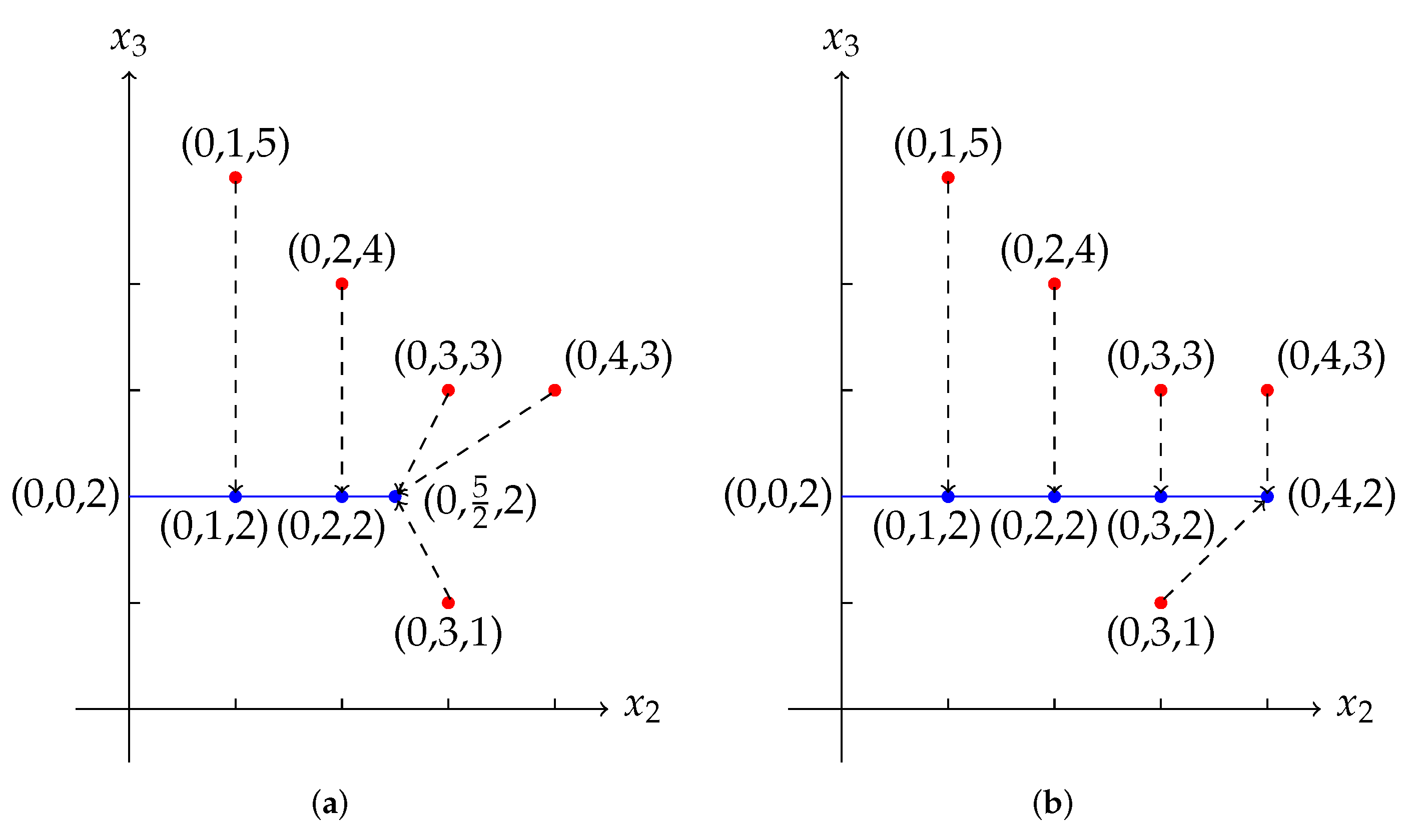
In this paper, we study the main question by focusing on tropical triangles (three-point tropical polytopes). Our goal is to develop an algorithm that can answer the main question with a high success rate. We develop one algorithm (Algorithm 1) and its improved version (Algorithm 2), such that for a given data set $X\subset {\mathbb{R}}^n/\mathbb{R}\mathbf{1}$, these algorithms output a tropical triangle $\mathcal{C}$, on which the projection of a Fermat-Weber point of X is a Fermat-Weber point of the projection of X. By sufficient experiments with random data sets, we show that Algorithms 1 and 2 can both succeed with a much higher probability than choosing a tropical triangle $\mathcal{C}$ randomly. We also show that the success rate of these two algorithms is stable while data sets are changing randomly. Algorithm 2 can output the result much faster than Algorithm 1 does averagely, because in most cases, Algorithm 2 correctly terminates with less steps than Algorithm 1 does (See Section 5). Our work can be viewed as a first step to an ambitious goal. We remark that, once the main question is completely solved, we can then ask how to characterize all nice tropical polytopes. Here, by a “nice tropical polytope”, we mean a tropical polytope, on which the projection of a Fermat-Weber point of a given data set X is a Fermat-Weber point of the projection of X. Then, we can use the nice tropical polytopes as principal components in the tropical PCA and possibly in other data analysis such as linear discriminant analysis.

Algorithm 1: First Version

Algorithm 2: Improved Version

This paper is organized as follows. In Section 2, we remind readers of the basic definitions in tropical geometry. In Section 3, we prove Theorem 1 and Theorem 2 for the correctness of the algorithms developed in this paper. In Section 4, we present Algorithms 1 and 2. We also explain how the algorithms work by two examples. In Section 5, we apply the algorithms developed in Section 4 on random data sets, and illustrate the experimental results.

2. Tropical Basics

In this section, we set up the notation throughout this paper, and prepare some basic tropical arithmetic and geometry (see more details in [20]). We will redefine our motivation in a precise way after Definition 6.

Definition 1 (Tropical Arithmetic Operations). 

We denote by $(\mathbb{R}\cup \{-\infty \},⊞,\odot )$ the max-plus tropical semi-ring. We define the tropical addition and thetropical multiplication as

$$c⊞d:=max\{c,d\},c\odot d:=c+d,\mathit{where}c,d\in \mathbb{R}\cup \{-\infty \}.$$

(1)

Definition 2 (Tropical Vector Addition). 

For any scalars $c,d\in \mathbb{R}\cup \{-\infty \}$, and for any vectors

$$\mathbf{u}=(u_1,\dots ,u_n),\mathbf{v}=(v_1,\dots ,v_n)\in {(\mathbb{R}\cup \{-\infty \})}^n,$$

(2)

we define the tropical vector addition as:

$$\begin{array}{cc}\hfill c\odot \mathbf{u}⊞d\odot \mathbf{v}& :=(max\{c+u_1,d+v_1\},\dots ,max\{c+u_n,d+v_n\}).\hfill \end{array}$$

(3)

Example 1.

Let

$$\mathbf{u}=(2,1,3),\mathbf{v}=(2,2,2).$$

(4)

Also we let $c=-2,d=1$. Then we have

$$c\odot \mathbf{u}⊞d\odot \mathbf{v}=(max\{-2+2,1+2\},max\{-2+1,1+2\},max\{-2+3,1+2\left\}\right)=(3,3,3).$$

(5)

For any point $\mathbf{u}\in {\mathbb{R}}^n$, we define the equivalence class $\left[\mathbf{u}\right]:=\{\mathbf{u}+c·\mathbf{1}|c\in \mathbb{R}\},\mathrm{where}\mathbf{1}=(1,\dots ,1).$ For instance, the vector $(3,3,3)$ is equivalent to (0,0,0). In the rest of this paper, we consider the tropical projective torus

$${\mathbb{R}}^n/\mathbb{R}\mathbf{1}:=\left\{\left[\mathbf{u}\right]\right|\mathbf{u}\in {\mathbb{R}}^n\}.$$

(6)

For convenience, we simply denote by $\mathbf{u}$ its equivalence class instead of $\left[\mathbf{u}\right]$, and we assume the first coordinate of every point in ${\mathbb{R}}^n/\mathbb{R}\mathbf{1}$ is 0. Because for any $\mathbf{u}=(u_1,\dots ,u_n)\in {\mathbb{R}}^n/\mathbb{R}\mathbf{1}$, it is equivalent to

$$\mathbf{u}=(0,u_2-u_1,\dots ,u_n-u_1).$$

(7)

Definition 3 (Tropical Distance). 

For any two points

$$\mathbf{u}=(u_1,\dots ,u_n),\mathbf{v}=(v_1,\dots ,v_n)\in {\mathbb{R}}^n/\mathbb{R}\mathbf{1},$$

(8)

we define the tropical distance$d_{tr}(\mathbf{u},\mathbf{v})$ as:

$$d_{tr}(\mathbf{u},\mathbf{v}):=max\left\{\right|u_i-v_i-u_j+v_j|:1\le i<j\le n\}=\underset{1\le i\le n}{max}\{u_i-v_i\}-\underset{1\le i\le n}{min}\{u_i-v_i\}.$$

(9)

Note that the tropical distance is a metric in ${\mathbb{R}}^n/\mathbb{R}\mathbf{1}$ [18] (Page 2030).

Example 2.

Let $\mathbf{u}=(0,4,2),\mathbf{v}=(0,1,1)\in {\mathbb{R}}^3/\mathbb{R}\mathbf{1}$. The tropical distance between $\mathbf{u}$, $\mathbf{v}$ is

$$d_{tr}(\mathbf{u},\mathbf{v})=max\{0,3,1\}-min\{0,3,1\}=3-0=3.$$

(10)

Definition 4 (Tropical Convex Hull). 

Given a finite subset

$$X=\{{\mathbf{x}}^{\left(1\right)},\dots ,{\mathbf{x}}^{\left(t\right)}\}\subset {\mathbb{R}}^n/\mathbb{R}\mathbf{1},$$

(11)

we define the tropical convex hull as the set of all tropical linear combinations of X:

$$tconv\left(X\right):=\{c_1\odot {\mathbf{x}}^{\left(1\right)}⊞c_2\odot {\mathbf{x}}^{\left(2\right)}⊞\dots ⊞c_t\odot {\mathbf{x}}^{\left(t\right)}|c_1,\dots ,c_t\in \mathbb{R}\}.$$

(12)

If $\left|X\right|=3,$ then the tropical convex hull of X is called a tropical triangle.

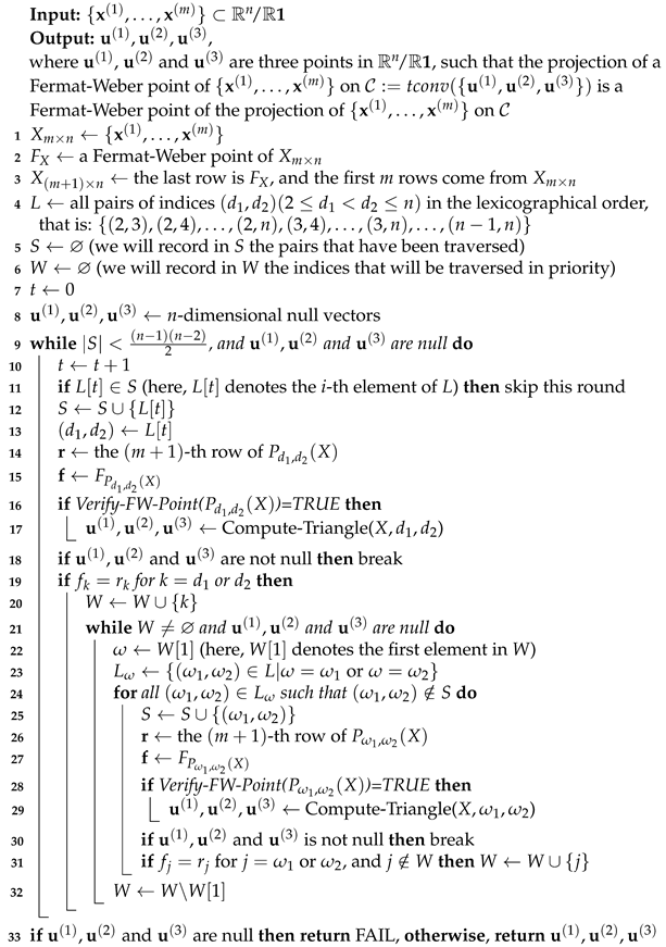
Example 3.

Consider a set $X=\{{\mathbf{x}}^{\left(1\right)},{\mathbf{x}}^{\left(2\right)},{\mathbf{x}}^{\left(3\right)}\}\subset {\mathbb{R}}^3/\mathbb{R}\mathbf{1}$, where

$${\mathbf{x}}^{\left(1\right)}=(0,0,0),{\mathbf{x}}^{\left(2\right)}=(0,4,2),{\mathbf{x}}^{\left(3\right)}=(0,2,4).$$

(13)

The tropical convex hull $tconv\left(X\right)$ is shown in Figure 1.

Definition 5 (Tropical Fermat-Weber Points). 

Suppose we have

$$X=\{{\mathbf{x}}^{\left(1\right)},\dots ,{\mathbf{x}}^{\left(t\right)}\}\subset {\mathbb{R}}^n/\mathbb{R}\mathbf{1}.$$

(14)

We define the set of tropical Fermat-Weber pointsof X as

$$\underset{\mathbf{y}\in {\mathbb{R}}^n/\mathbb{R}\mathbf{1}}{argmin}\sum _{i=1}^t{d}_{tr}(\mathbf{y},{\mathbf{x}}^{\left(i\right)}).$$

(15)

The Fermat-Weber point of X is denoted by $F_X$.

Proposition 1

([18], Proposition 25). Given $X=\{{\mathbf{x}}^{\left(1\right)},\dots ,{\mathbf{x}}^{\left(t\right)}\}\subset {\mathbb{R}}^n/\mathbb{R}\mathbf{1}$, the set of tropical Fermat-Weber points of X in ${\mathbb{R}}^n/\mathbb{R}\mathbf{1}$ is a convex polytope in ${\mathbb{R}}^{n-1}$. It consists of all optimal solutions $\mathbf{y}=(y_1,\dots ,y_n)$ to the linear programming problem:

$$\begin{array}{c}\mathit{minimize}\sum _{i=1}^t{\gamma }_i,\hfill \\ \hfill \mathit{subject}\mathit{to}{\gamma }_i& \ge y_k-x_k^{\left(i\right)}-y_{\ell }+x_{\ell }^{\left(i\right)},\hfill \\ \hfill {\gamma }_i& \ge -(y_k-x_k^{\left(i\right)}-y_{\ell }+x_{\ell }^{\left(i\right)}),\hfill \\ \hfill \mathit{for}\mathit{all}1\le k<\ell & \le n,\mathit{and}\mathit{for}\mathit{all}i\in \{1,2,\dots ,t\}.\hfill \end{array}$$

(16)

Definition 6 (Tropical Projection). 

Let

$$U=\{{\mathbf{u}}^{\left(1\right)}=(u_1^{\left(1\right)},\dots ,u_n^{\left(1\right)}),\dots ,{\mathbf{u}}^{\left(t\right)}=(u_1^{\left(t\right)},\dots ,u_n^{\left(t\right)})\}\subset {\mathbb{R}}^n/\mathbb{R}\mathbf{1}.$$

(17)

Also let $\mathcal{C}=tconv\left(U\right)$. For any point $\mathbf{x}=(x_1,\dots ,x_n)\in {\mathbb{R}}^n/\mathbb{R}\mathbf{1}$, we define the projection of $\mathbf{x}$ on $\mathcal{C}$ as:

$${\delta }_{\mathcal{C}}\left(\mathbf{x}\right):={\lambda }_1\odot {\mathbf{u}}^{\left(1\right)}⊞{\lambda }_2\odot {\mathbf{u}}^{\left(2\right)}⊞\cdots ⊞{\lambda }_t\odot {\mathbf{u}}^{\left(t\right)},$$

(18)

where ${\lambda }_i:=min\{x_1-u_1^{\left(i\right)},\dots ,x_n-u_n^{\left(i\right)}\}$ for all $i\in \{1,\dots ,t\}$ [23] (Formula 3.3).

Now we are prepared to repeat the main question in a precise way: for a given data set X, how to find a tropical triangle $\mathcal{C}$ such that the following equality holds

$${\delta }_{\mathcal{C}}\left(F_X\right)=F_{\{{\delta }_{\mathcal{C}}\left({\mathbf{x}}^{\left(1\right)}\right),\dots ,{\delta }_{\mathcal{C}}\left({\mathbf{x}}^{\left(t\right)}\right)\}}.$$

(19)

The above question is motivated by the fact that the equality (19) does not hold for any tropical triangle $\mathcal{C}$ (see Example 4). It is remarkable that the Fermat-Weber point might not be unique. The following Proposition 2 indicates that for some special data sets, the Fermat-Weber point is unique. But even for these special sets, the equality (19) still does not hold for any tropical triangle (see Example 5). In the rest of this paper, we will develop algorithms for automatically searching tropical triangles such that the equality (19) holds.

Proposition 2

([24], Lemma 8). Let $X=\{{\mathbf{x}}^{\left(1\right)},\dots ,{\mathbf{x}}^{\left(m\right)}\}\subset {\mathbb{R}}^n/\mathbb{R}\mathbf{1}$. Suppose $F_X$ is a Fermat-Weber point of X. Then $\{F_X,{\mathbf{x}}^{\left(1\right)},\dots ,{\mathbf{x}}^{\left(m\right)}\}$ has exactly one Fermat-Weber point, which is $F_X$.

Examples

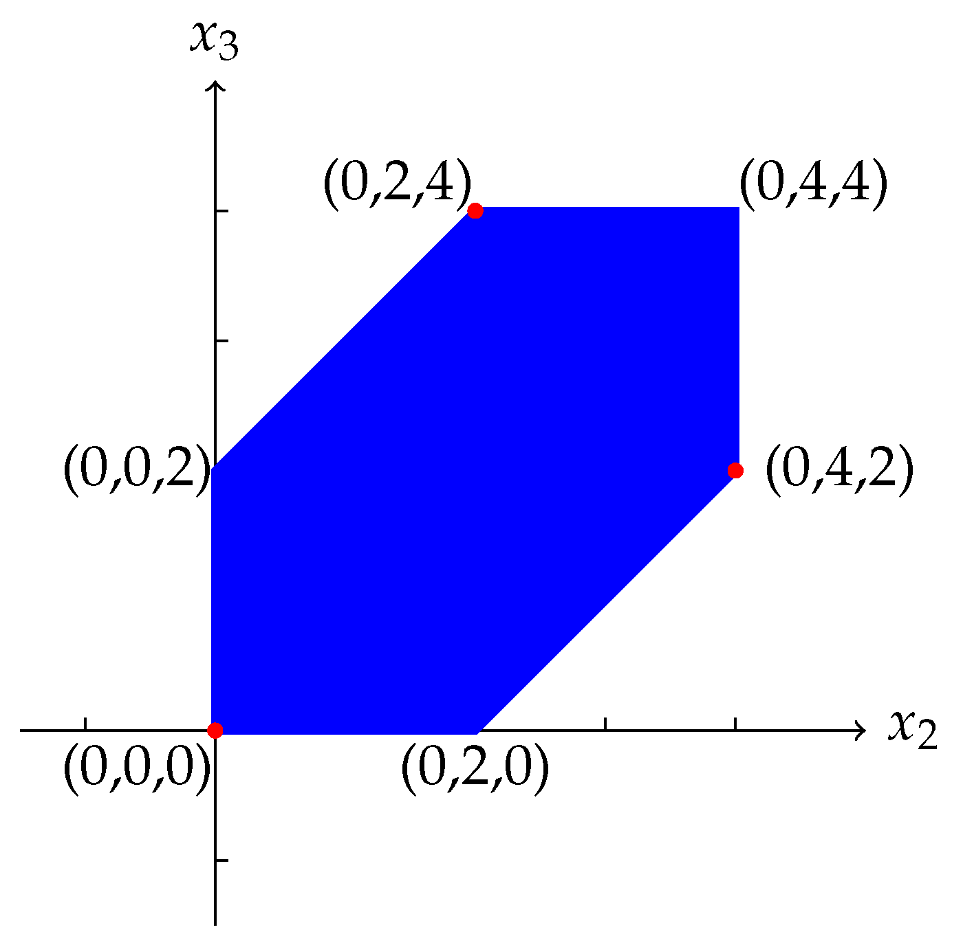
Example 4.

This example shows that, for a given data set $X\subset {\mathbb{R}}^3/\mathbb{R}\mathbf{1}$ and a given two-point tropical polytope $\mathcal{C}$, the projection of a Fermat-Weber point of X on $\mathcal{C}$ is not necessarily a Fermat-Weber point of the projection of X on $\mathcal{C}$.

Suppose we have $X=\{(0,1,5),(0,2,4),(0,3,1),(0,4,3)\}\subset {\mathbb{R}}^3/\mathbb{R}\mathbf{1}.$ By solving the linear programming (16) in Proposition 1 (e.g., usinglpSolveinR), we obtain that, $(0,3,3)$ is a Fermat-Weber point of X. Let $\mathcal{C}=tconv\left(\{(0,0,2),(0,\frac{33}{10},2)\}\right).$ Then the projection of X on $\mathcal{C}$ is $P=\{(0,1,2),(0,2,2),(0,\frac{33}{10},2)\}.$

We remark that, in P, $(0,1,2)$ is the projection of $(0,1,5)$, $(0,2,2)$ is the projection of $(0,2,4)$, and $(0,\frac{33}{10},2)$ is the projection of both $(0,3,1)$ and $(0,4,3)$ on $\mathcal{C}$.

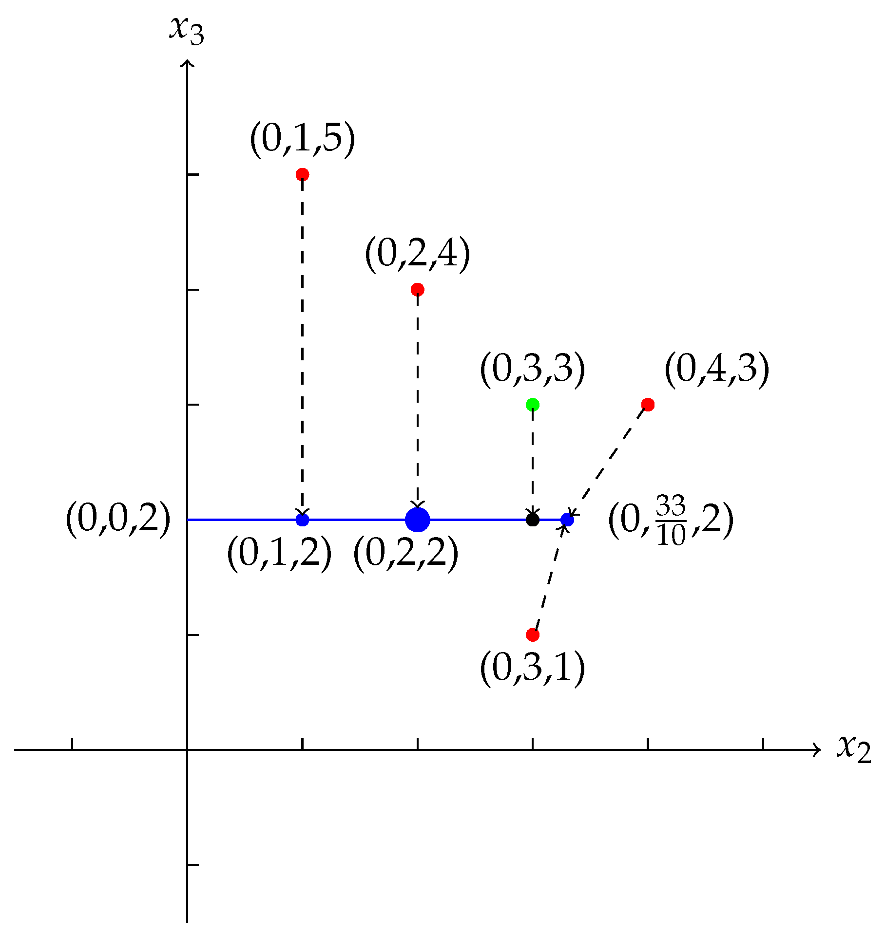
Note that $(0,2,2)$ is the unique Fermat-Weber point of P, while the projection of a Fermat-Weber point $(0,3,3)$ of X is $(0,3,2)$. So we can see that the projection of a Fermat-Weber point of X on $\mathcal{C}$ is not a Fermat-Weber point of the projection. In Figure 2, the red points are the points in X. The green point is a Fermat-Weber point of X. The blue line segment is the tropical convex hull $\mathcal{C}$ generated by $(0,0,2)$ and $(0,\frac{33}{10},2)$. The blue points are the projection P of X. And the biggest blue one $(0,2,2)$ is the Fermat-Weber point of P. The black point $(0,3,2)$ is the projection of the green point.

Example 5.

This example shows that, in ${\mathbb{R}}^n/\mathbb{R}\mathbf{1}$, if a set $\tilde{X}$ is the union of X and a Fermat-Weber point $F_X$ of X, then it is not guaranteed that the projection of the Fermat-Weber point $F_X$ of $\tilde{X}$ is a Fermat-Weber point of the projection of $\tilde{X}$. Besides, whether the projection of the Fermat-Weber point $F_X$ of $\tilde{X}$ is a Fermat-Weber point of the projection of $\tilde{X}$ depends on the choice of the tropical convex hull $\mathcal{C}$.

Suppose we have

$$X=\{(0,1,5),(0,2,4),(0,3,1),(0,4,3)\}\subset {\mathbb{R}}^3/\mathbb{R}\mathbf{1}.$$

(20)

By solving the linear programming (16) in Proposition 1, we obtain that, $(0,3,3)$ is a Fermat-Weber point of X. Then

$$\tilde{X}=X\cup \left\{F_X\right\}=\{(0,1,5),(0,2,4),(0,3,1),(0,4,3),(0,3,3)\}.$$

(21)

Let ${\mathcal{C}}_1=tconv\left(\{(0,0,2),(0,\frac{5}{2},2)\}\right),{\mathcal{C}}_2=tconv\left(\{(0,0,2),(0,4,2)\}\right).$$P_1$ and $P_2$ are the projection of $\tilde{X}$ on ${\mathcal{C}}_1$ and ${\mathcal{C}}_2$ respectively, where

$$P_1=\{(0,1,2),(0,2,2),(0,\frac{5}{2},2)\},P_2=\{(0,1,2),(0,2,2),(0,3,2),(0,4,2)\}.$$

(22)

We remark that, in $P_1$, $(0,1,2)$ is the projection of $(0,1,5)$, $(0,2,2)$ is the projection of $(0,2,4)$, and $(0,\frac{5}{2},2)$ is the projection of $(0,3,1)$, $(0,4,3)$ and $(0,3,3)$ on ${\mathcal{C}}_1$. And in $P_2$, $(0,1,2)$ is the projection of $(0,1,5)$, $(0,2,2)$ is the projection of $(0,2,4)$, $(0,3,2)$ is the projection of $(0,3,3)$, and $(0,4,2)$ is the projection of $(0,3,1)$ and $(0,4,3)$ on ${\mathcal{C}}_2$.

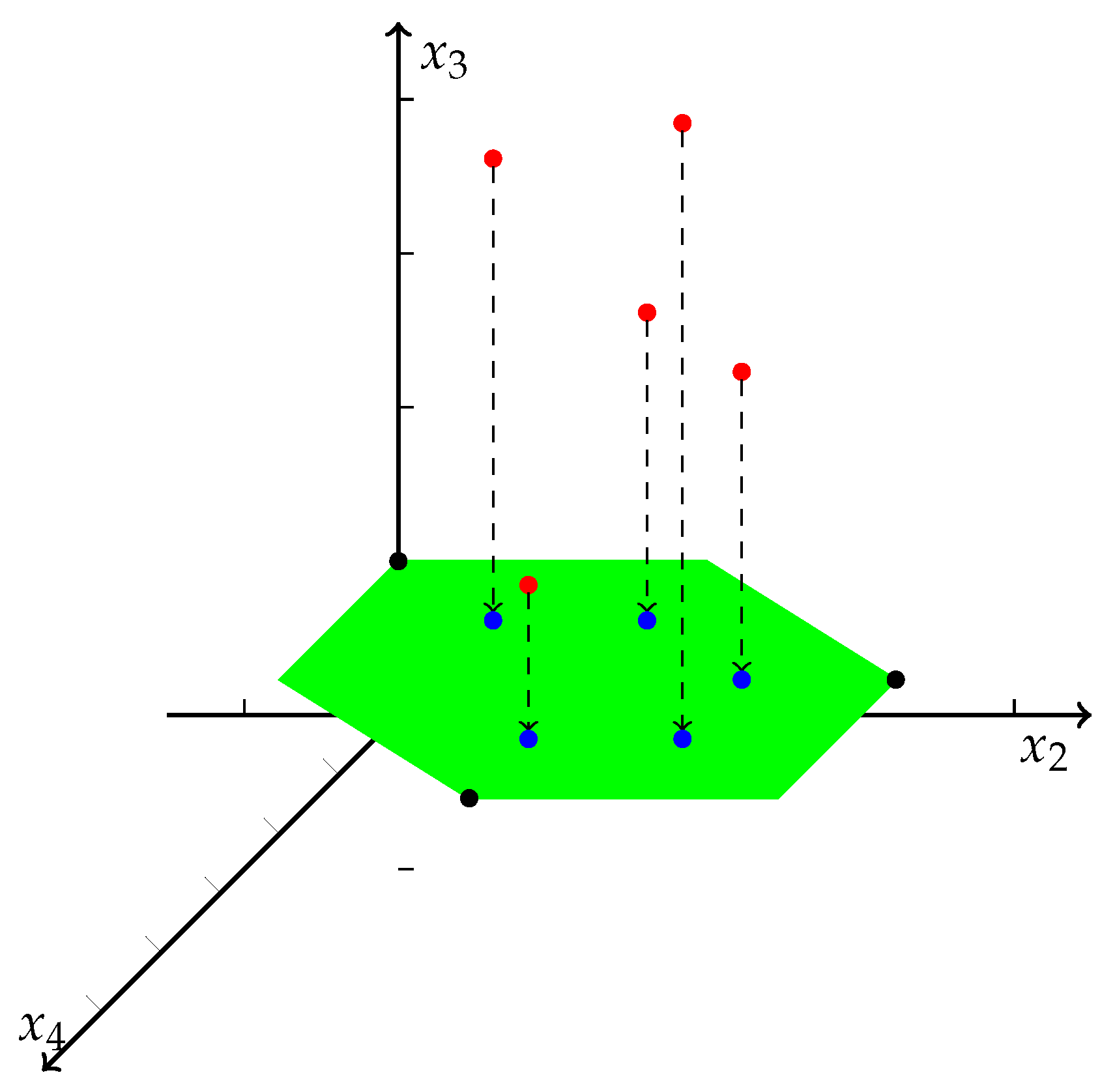
Note that $(0,2,2)$ is the unique Fermat-Weber point of $P_1$, while the projection of the Fermat-Weber point $(0,3,3)$ of $\tilde{X}$ on ${\mathcal{C}}_1$ is $(0,\frac{5}{2},2)$. So we can see that the projection of the Fermat-Weber point of $\tilde{X}$ on ${\mathcal{C}}_1$ is not a Fermat-Weber point of the projection. On the other hand, the projection of the Fermat-Weber point $(0,3,3)$ on ${\mathcal{C}}_2$ is $(0,3,2)$, which is exactly a Fermat-Weber point of the projection. In the panel (a) of Figure 3, the points in $\tilde{X}$ are red. The projection points of $\tilde{X}$ are blue. The blue line segment is the tropical convex hull generated by $(0,0,2)$ and $(0,\frac{5}{2},2)$. The blue points are the projection $P_1$ of $\tilde{X}$. Note that $(0,\frac{5}{2},2)$ is the projection of the Fermat-Weber point $(0,3,3)$ of $\tilde{X}$, and $(0,2,2)$ is the unique Fermat-Weber point of $P_1$. In the panel (b) of Figure 3, the points in $\tilde{X}$ are red. The projection points of $\tilde{X}$ are blue. The blue line segment is the tropical convex hull generated by $(0,0,2)$ and $(0,4,2)$. The blue points are the projection $P_2$ of $\tilde{X}$. Note that $(0,3,2)$ is the projection of the Fermat-Weber point $(0,3,3)$ of $\tilde{X}$, which is a Fermat-Weber point of $P_2$.

3. Theorems

In this section, we introduce Theorems 1 and 2 for proving the correctness of the algorithms developed in the next section.

Lemma 1.

Suppose we have a data set

$$X=\{{\mathbf{x}}^{\left(1\right)}=(x_1^{\left(1\right)},x_2^{\left(1\right)},\dots ,x_n^{\left(1\right)}),\dots ,{\mathbf{x}}^{\left(m\right)}=(x_1^{\left(m\right)},x_2^{\left(m\right)},\dots ,x_n^{\left(m\right)})\}\subset {\mathbb{R}}^n/\mathbb{R}\mathbf{1}.$$

(23)

Let t be a number which is no more than

$$\underset{1\le k\le m}{min}\underset{1\le \ell \le n}{min}\left\{x_{\ell }^{\left(k\right)}\right\}.$$

(24)

For any two fixed integers $d_1\mathrm{and}{d}_2(2\le d_1<d_2\le n)$, we define three points ${\mathbf{u}}^{\left(1\right)},{\mathbf{u}}^{\left(2\right)},{\mathbf{u}}^{\left(3\right)}\in {\mathbb{R}}^n/\mathbb{R}\mathbf{1}$ as follows.

$$\begin{array}{cccc}\mathit{for}k=1,2,3,\hfill & \hfill & \hfill u_1^{\left(k\right)}& :=0,\hfill \end{array}$$

(25)

$$\begin{array}{cccc}\hfill & u_{d_1}^{\left(1\right)}:=\underset{1\le k\le m}{min}\left\{x_{d_1}^{\left(k\right)}\right\}-1,\hfill & \hfill u_{d_2}^{\left(1\right)}& :=\underset{1\le k\le m}{min}\left\{x_{d_2}^{\left(k\right)}\right\}-1,\hfill \end{array}$$

(26)

$$\begin{array}{cccc}\hfill & u_{d_1}^{\left(2\right)}:=\underset{1\le k\le m}{min}\left\{x_{d_1}^{\left(k\right)}\right\}+1,\hfill & \hfill u_{d_2}^{\left(2\right)}& :=\underset{1\le k\le m}{max}\left\{x_{d_2}^{\left(k\right)}\right\}+1,\hfill \end{array}$$

(27)

$$\begin{array}{cccc}\hfill & u_{d_1}^{\left(3\right)}:=\underset{1\le k\le m}{max}\left\{x_{d_1}^{\left(k\right)}\right\}+1,\hfill & \hfill u_{d_2}^{\left(3\right)}& :=\underset{1\le k\le m}{min}\left\{x_{d_2}^{\left(k\right)}\right\}+1,\hfill \end{array}$$

(28)

$$\begin{array}{cccc}\hfill & \mathit{for}k=1,2,3,\mathit{and}\mathit{for}\mathit{all}\ell \ne 1,d_1,d_2,\hfill & \hfill u_{\ell }^{\left(k\right)}& :=t.\hfill \end{array}$$

(29)

Let $\mathcal{C}=tconv\left(\{{\mathbf{u}}^{\left(1\right)},{\mathbf{u}}^{\left(2\right)},{\mathbf{u}}^{\left(3\right)}\}\right)$. Then, the projection of X on $\mathcal{C}$ is

$${\delta }_{\mathcal{C}}\left({\mathbf{x}}^{\left(k\right)}\right)=(0,t,\dots ,t,x_{d_1}^{\left(k\right)},t,\dots ,t,x_{d_2}^{\left(k\right)},t,\dots ,t),\mathrm{for}\mathrm{all}k\in \{1,2,\dots ,m\},$$

(30)

where $x_{d_1}^{\left(k\right)}$ and $x_{d_2}^{\left(k\right)}$ are respectively located at the $d_1$-th and $d_2$-th coordinates of ${\delta }_{\mathcal{C}}\left({\mathbf{x}}^{\left(k\right)}\right)$.

Proof. 

Recall that we assume the first coordinate of every point in ${\mathbb{R}}^n/\mathbb{R}\mathbf{1}$ is 0. For any

$${\mathbf{x}}^{\left(i\right)}=(x_1^{\left(i\right)},x_2^{\left(i\right)},\dots ,x_n^{\left(i\right)})\in X,$$

(31)

by Definition 6, we have that ${\lambda }_i$ in (18) should be:

$${\lambda }_1=0,{\lambda }_2=x_{d_2}^{\left(i\right)}-\underset{1\le k\le m}{max}\left\{x_{d_2}^{\left(k\right)}\right\}-1,{\lambda }_3=x_{d_1}^{\left(i\right)}-\underset{1\le k\le m}{max}\left\{x_{d_1}^{\left(k\right)}\right\}-1.$$

(32)

Then the conclusion follows from (18). □

Suppose X is the data set stated in Lemma 1. For ${\mathbf{u}}^{\left(1\right)}$, ${\mathbf{u}}^{\left(2\right)}$ and ${\mathbf{u}}^{\left(3\right)}$ in Lemma 1, let $\mathcal{C}=tconv\left(\{{\mathbf{u}}^{\left(1\right)},{\mathbf{u}}^{\left(2\right)},{\mathbf{u}}^{\left(3\right)}\}\right)$, we have the following remarks: the equalities (26)–(28) make sure that the tropical triangle $\mathcal{C}$ is big enough; the equalities (25) and (29) make sure that $\mathcal{C}$ parallels with a coordinate plane; the equality (29) makes sure that $\mathcal{C}$ is located under all points in X. Lemma 1 shows that we can project X vertically onto $\mathcal{C}$ (see Example 6 and Figure 4).

Example 6.

Suppose we have

$$X=\{(0,2,3,1),(0,1,4,1),(0,3,3,2),(0,3,5,3),(0,2,2,3)\}\subset {\mathbb{R}}^4/\mathbb{R}\mathbf{1}.$$

(33)

Let $t=1$. Fix $d_1=2,\mathrm{and}{d}_2=4$. By (25)–(29), we can define three points ${\mathbf{u}}^{\left(1\right)},{\mathbf{u}}^{\left(2\right)},\mathrm{and}{\mathbf{u}}^{\left(3\right)}$ as:

$${\mathbf{u}}^{\left(\mathbf{1}\right)}=(0,0,1,0),{\mathbf{u}}^{\left(\mathbf{2}\right)}=(0,2,1,4),{\mathbf{u}}^{\left(\mathbf{3}\right)}=(0,4,1,2).$$

(34)

Let $\mathcal{C}=tconv\left(\{{\mathbf{u}}^{\left(\mathbf{1}\right)},{\mathbf{u}}^{\left(\mathbf{2}\right)},{\mathbf{u}}^{\left(\mathbf{3}\right)}\}\right)$ (see the green region in Figure 4). Then, by Lemma 1, the projection points of X on $\mathcal{C}$ are shown in Figure 4 (see the blue points).

Definition 7 (Data Matrix). 

We define any matrix X with n columns as adata matrix, where each row of X is regarded as a point in ${\mathbb{R}}^n/\mathbb{R}\mathbf{1}$.

Below we denote by $X_{m\times n}$ the data matrix X with size $m\times n$.

Definition 8 (Fermat-Weber Points of a Data Matrix). 

For a given data matrix $X_{m\times n}$, suppose the i-th row of X is ${\mathbf{x}}^{\left(i\right)}$ ($i\in \{1,\dots ,m\}$). We define theFermat-Weber point ofX as the Fermat-Weber point of $\{{\mathbf{x}}^{\left(1\right)},\dots ,{\mathbf{x}}^{\left(m\right)}\}$. We still denote by $F_X$ the Fermat-Weber point of X.

Definition 9 (Projection Matrix). 

For a given data matrix $X_{m\times n}$, and for any two fixed integers $d_1\mathrm{and}{d}_2(2\le d_1<d_2\le n)$, we define the projection matrix of X (denoted by $P_{d_1,d_2}\left(X\right)$) as a matrix with size $m\times n$, such that for all $k\in \{1,\dots ,m\}$, the $k-th$ row of $P_{d_1,d_2}\left(X\right)$ is

$$(0,t,\dots ,t,x_{d_1}^{\left(k\right)},t,\dots ,t,x_{d_2}^{\left(k\right)},t,\dots ,t),$$

(35)

where

• $x_{d_1}^{\left(k\right)}$ and $x_{d_2}^{\left(k\right)}$ are respectively the $(k,d_1)$-entry and the $(k,d_2)$-entry of X, and are respectively located at the $(k,d_1)$-entry and the $(k,d_2)$-entry of of $P_{d_1,d_2}\left(X\right)$.
• t is a fixed number, such that $t=\underset{1\le k\le m}{min}\underset{1\le \ell \le n}{min}\left\{(k,\ell )-\mathrm{entry}\mathrm{of}X\right\}$.

Note that the projection matrix $P_{d_1,d_2}\left(X\right)$ is still a data matrix.

Recall the Proposition 2 tells that, if $F_X$ is a Fermat-Weber point of $X=\{{\mathbf{x}}^{\left(1\right)},\dots ,{\mathbf{x}}^{\left(m\right)}\}$ $\subset {\mathbb{R}}^n/\mathbb{R}\mathbf{1}$, then $F_X$ is the unique Fermat-Weber point of $\{F_X,{\mathbf{x}}^{\left(1\right)},\dots ,{\mathbf{x}}^{\left(m\right)}\}$.

Theorem 1.

Suppose we have a data matrix $X_{(m+1)\times n}$, where the last row of X is a Fermat-Weber point of the matrix made by the first m rows of X. We fix two integers $d_1$ and $d_2(2\le d_1<d_2\le n)$. Let $\mathbf{r}$ be the last row of $P_{d_1,d_2}\left(X\right)$.

If $\mathbf{r}$ is a Fermat-Weber point of $P_{d_1,d_2}\left(X\right)$, and ${\mathbf{u}}^{\left(1\right)}$, ${\mathbf{u}}^{\left(2\right)}$ and ${\mathbf{u}}^{\left(3\right)}$ are defined by (25)–(29), then the projection of the Fermat-Weber point of X on $tconv\left(\{{\mathbf{u}}^{\left(1\right)},{\mathbf{u}}^{\left(2\right)},{\mathbf{u}}^{\left(3\right)}\}\right)$ is a Fermat-Weber point of the projection of X on $tconv\left(\{{\mathbf{u}}^{\left(1\right)},{\mathbf{u}}^{\left(2\right)},{\mathbf{u}}^{\left(3\right)}\}\right)$.

Proof. 

By Lemma 1 and Definition 9 we know that, the projection of X on

$$\mathcal{C}:=tconv\left(\{{\mathbf{u}}^{\left(1\right)},{\mathbf{u}}^{\left(2\right)},{\mathbf{u}}^{\left(3\right)}\}\right)$$

(36)

is $P_{d_1,d_2}\left(X\right)$. Note that the last row of X is the unique Fermat-Weber point of X. Also note that $\mathbf{r}$ is the projection of the last row of X. Then by the assumption that $\mathbf{r}$ is a Fermat-Weber point of $P_{d_1,d_2}\left(X\right)$ we know that, the projection of the Fermat-Weber point of X on $\mathcal{C}$ is a Fermat-Weber point of the projection of X on $\mathcal{C}$. □

Theorem 2.

Suppose we have a data matrix $X_{m\times n}$. We fix two integers $d_1$ and $d_2(2\le d_1<d_2\le n)$. Let $\mathbf{r}$ be a point

$$(0,t,\dots ,t,r_{d_1},t,\dots ,t,r_{d_2},t,\dots ,t),$$

(37)

where $r_{d_1}$ and $r_{d_2}$ are undetermined numbers, and t is the smallest entry of X. Let $\mathbf{f}$ be a Fermat-Weber point of $P_{d_1,d_2}\left(X\right)$. If $r_{d_1}=f_{d_1},$ and $r_{d_2}=f_{d_2},$ then $\mathbf{r}$ is a Fermat-Weber point of $P_{d_1,d_2}\left(X\right)$.

Proof. 

By Definition 9, the i-th row of $P_{d_1,d_2}\left(X\right)$ has the form

$${\mathbf{p}}^{\left(\mathbf{i}\right)}:=(0,t,\dots ,t,x_{d_1}^{\left(i\right)},t,\dots ,t,x_{d_2}^{\left(i\right)},t,\dots ,t),\mathrm{for}\mathrm{all}i\in \{1,\dots ,m\}.$$

(38)

Assume that $\mathbf{f}=(0,f_2,\dots ,f_n)$ is a Fermat-Weber point of $P_{d_1,d_2}\left(X\right)$. Suppose there exists $k\in S:=\{1,\dots ,n\}\backslash \{1,d_1,d_2\},$ such that $f_k\ne t.$ For any $i\in \{1,\dots ,m\}$, let

$$\begin{array}{cc}\hfill & A_i=min\{0,f_{d_1}-x_{d_1}^{\left(i\right)},f_{d_2}-x_{d_2}^{\left(i\right)}\},\hfill \end{array}$$

(39)

$$\begin{array}{cc}\hfill & B_i=max\{0,f_{d_1}-x_{d_1}^{\left(i\right)},f_{d_2}-x_{d_2}^{\left(i\right)}\}.\hfill \end{array}$$

(40)

Then we have

$$\begin{array}{c}\hfill \sum _{i=1}^m{d}_{tr}({\mathbf{p}}^{\left(i\right)},\mathbf{r})=\sum _{i=1}^m(B_i-A_i),\sum _{i=1}^m{d}_{tr}({\mathbf{p}}^{\left(i\right)},\mathbf{f})=\sum _{i=1}^m\left(\underset{k\in S}{max}\{B_i,f_k-t\}-\underset{k\in S}{min}\{A_i,f_k-t\}\right).\end{array}$$

(41)

It is easy to see that ${\displaystyle \sum _{i=1}^m}{d}_{tr}({\mathbf{p}}^{\left(i\right)},\mathbf{f})\ge {\displaystyle \sum _{i=1}^m}{d}_{tr}({\mathbf{p}}^{\left(i\right)},\mathbf{r}).$ So, by Definition 5, $\mathbf{r}$ is a Fermat-Weber point of $P_{d_1,d_2}\left(X\right).$ □

4. Algorithms

In this section, we develop Algorithms 1 and 2, such that for a given data set $X\subset {\mathbb{R}}^n/\mathbb{R}\mathbf{1}$, these two algorithms output a tropical triangle $\mathcal{C}$, on which the projection of a Fermat-Weber point of X is a Fermat-Weber point of the projection of X.

The input of Algorithms 1 and 2 is a data set

$$\{{\mathbf{x}}^{\left(1\right)},\dots ,{\mathbf{x}}^{\left(m\right)}\}\subset {\mathbb{R}}^n/\mathbb{R}\mathbf{1}.$$

(42)

Algorithms 1 and 2 output three points

$${\mathbf{u}}^{\left(1\right)},{\mathbf{u}}^{\left(2\right)},{\mathbf{u}}^{\left(3\right)}\in {\mathbb{R}}^n/\mathbb{R}\mathbf{1},$$

(43)

such that the projection of a Fermat-Weber point of $\{{\mathbf{x}}^{\left(1\right)},\dots ,{\mathbf{x}}^{\left(m\right)}\}$ on

$$\mathcal{C}:=tconv\left(\{{\mathbf{u}}^{\left(1\right)},{\mathbf{u}}^{\left(2\right)},{\mathbf{u}}^{\left(3\right)}\}\right)$$

(44)

is a Fermat-Weber point of the projection of $\{{\mathbf{x}}^{\left(1\right)},\dots ,{\mathbf{x}}^{\left(m\right)}\}$ on $\mathcal{C}$.

There are two main steps in each algorithm as follows.

• Step 1. We define a data matrix X, such that for all $i\in \{1,\dots ,m\},$ the i-th row of X is ${\mathbf{x}}^{\left(i\right)}.$ We obtain a Fermat-Weber point $F_X$ by solving the linear programming (16). We define a matrix $\tilde{X}$ with size $(m+1)\times n$, such that the last row of $\tilde{X}$ is $F_X$, and the first m rows of $\tilde{X}$ come from X.
• Step 2. We traverse all pairs $(d_1,d_2)$ such that $2\le d_1<d_2\le n$, and we calculate the projection matrix $P_{d_1,d_2}\left(\tilde{X}\right)$ by Definition 9. Check if the last row of $P_{d_1,d_2}\left(\tilde{X}\right)$ is a Fermat-Weber point of $P_{d_1,d_2}\left(\tilde{X}\right)$. If so, we calculate the three points ${\mathbf{u}}^{\left(1\right)},{\mathbf{u}}^{\left(2\right)}\mathrm{and}{\mathbf{u}}^{\left(3\right)}$ by (25)–(29) in Lemma 1, return the output, and terminate. By Theorem 1 we know that, the projection of a Fermat-Weber point of X on $\mathcal{C}=tconv\left(\{{\mathbf{u}}^{\left(1\right)},{\mathbf{u}}^{\left(2\right)},{\mathbf{u}}^{\left(3\right)}\}\right)$ is a Fermat-Weber point of the projection of X on $\mathcal{C}.$ If for all $(d_1,d_2)$, the last row of $P_{d_1,d_2}\left(\tilde{X}\right)$ is not a Fermat-Weber point of $P_{d_1,d_2}\left(\tilde{X}\right)$, then return FAIL.

Remark 1.

It is not guaranteed that Algorithms 1 and 2 will always succeed (return the tropical triangle). If the algorithms succeed, then by Theorem 1, Algorithm 1 is correct, and by Theorems 1 and 2, Algorithm 2 is correct.

Algorithms 1 and 2 always succeed or fail simultaneously. But our experimental results in the next section show that, Algorithm 1 or Algorithm 2 succeeds with a much higher probability than choosing tropical triangles randomly. Our experimental results also show that, if Algorithms 1 and 2 succeed, then with the probability more than $50\%$, Algorithm 2 would terminate in less traversal steps than Algorithm 1 does (see Section 5).

Remark that, the difference between Algorithms 1 and 2 is the traversal strategy, i.e., the Step 2. is different. Below we give more details about Step 2.

Let

$$L=\left\{\right(2,3),(2,4),\dots ,(2,n),(3,4),(3,5),\dots ,(3,n),\dots ,(n-1,n\left)\right\}.$$

(45)

1.

In Algorithm 1: Step 2.,we traverse all pairs $(d_1,d_2)$ ($2\le d_1<d_2\le n$) in L one by one, i.e., we traverse the pairs in the lexicographical order.

2.

In Algorithm 2: Step 2., we consider the same L defined in (45). Note that $\left|L\right|=\frac{(n-1)(n-2)}{2}$. Let W and S be two empty sets. In the future, we will record in W some indices that will be traversed in priority, and record in S the pairs that have been traversed. Let ${\mathbf{u}}^{\left(1\right)}$, ${\mathbf{u}}^{\left(2\right)}$ and ${\mathbf{u}}^{\left(3\right)}$ be null vectors.

Now we start a loop (see lines 2–2 in Algorithm 2). In this loop, we traverse all pairs in L while $\left|S\right|<\frac{(n-1)(n-2)}{2}$, and ${\mathbf{u}}^{\left(1\right)}$, ${\mathbf{u}}^{\left(2\right)}$ and ${\mathbf{u}}^{\left(3\right)}$ are null. For each pair $(d_1,d_2)\in L$, if $(d_1,d_2)\in S$, then we skip the pair. If $(d_1,d_2)\notin S$, then we add the pair into S, and calculate the projection matrix $P_{d_1,d_2}\left(\tilde{X}\right)$ by Definition 9. Let $\mathbf{r}$ be the last row of $P_{d_1,d_2}\left(\tilde{X}\right)$. If $\mathbf{r}$ is a Fermat-Weber point of $P_{d_1,d_2}\left(\tilde{X}\right)$, then we calculate ${\mathbf{u}}^{\left(1\right)}$, ${\mathbf{u}}^{\left(2\right)}$ and ${\mathbf{u}}^{\left(3\right)}$ by formulas (25)–(29) in Lemma 1, return the output and terminate. By Theorem 1 we know that, the projection of a Fermat-Weber point of X on $\mathcal{C}:=tconv\left(\{{\mathbf{u}}^{\left(1\right)},{\mathbf{u}}^{\left(2\right)},{\mathbf{u}}^{\left(3\right)}\}\right)$ is a Fermat-Weber point of the projection of X on $\mathcal{C}.$ If $\mathbf{r}$ is not a Fermat-Weber point of $P_{d_1,d_2}\left(\tilde{X}\right)$, then by Theorem 2, at most one of the following two equalities holds:

$$\begin{array}{cc}\hfill & r_{d_1}=f_{d_1},\hfill \end{array}$$

(46)

$$\begin{array}{cc}\hfill & r_{d_2}=f_{d_2},\hfill \end{array}$$

(47)

where $\mathbf{f}$ is a Fermat-Weber point of $P_{d_1,d_2}\left(\tilde{X}\right).$ So we have 3 cases.

• (Case 1) If only (46) holds, then we add $d_1$ into W, and stop doing the traversal of L.
• (Case 2) If only (47) holds, then we add $d_2$ into W, and stop doing the traversal of L.
• (Case 3) If neither (46) nor (47) holds, then we move on to the next pair in L.

Now we explain what we do if (Case 1) happens ((Case 2) is similar). Note that W is nonempty at this time, and ${\mathbf{u}}^{\left(1\right)}$, ${\mathbf{u}}^{\left(2\right)}$ and ${\mathbf{u}}^{\left(3\right)}$ are null. For each element $\omega \in W$, we define

$$L_{\omega }=\{({\omega }_1,{\omega }_2)\in L|{\omega }_1=\omega \mathrm{or}{\omega }_2=\omega \}.$$

(48)

We start traversing all pairs in $L_{\omega }$. For each pair $({\omega }_1,{\omega }_2)\in L_{\omega }$, if $({\omega }_1,{\omega }_2)\in S$, then we skip the pair. If $({\omega }_1,{\omega }_2)\notin S$, then we add the pair into S, and calculate the projection matrix $P_{{\omega }_1,{\omega }_2}\left(\tilde{X}\right)$ by Definition 9. Let $\mathbf{r}$ be the last row of $P_{{\omega }_1,{\omega }_2}\left(\tilde{X}\right)$. If $\mathbf{r}$ is a Fermat-Weber point of $P_{{\omega }_1,{\omega }_2}\left(\tilde{X}\right)$, then calculate ${\mathbf{u}}^{\left(1\right)}$, ${\mathbf{u}}^{\left(2\right)}$ and ${\mathbf{u}}^{\left(3\right)}$ by formulas (25)–(29) in Lemma 1, output ${\mathbf{u}}^{\left(1\right)}$, ${\mathbf{u}}^{\left(2\right)}$ and ${\mathbf{u}}^{\left(3\right)}$, and terminate. If $\mathbf{r}$ is not a Fermat-Weber point of $P_{{\omega }_1,{\omega }_2}\left(\tilde{X}\right)$, then by Theorem 2, at most one of the following two equalities holds:

$$\begin{array}{cc}\hfill & r_{{\omega }_1}=f_{{\omega }_1},\hfill \end{array}$$

(49)

$$\begin{array}{cc}\hfill & r_{{\omega }_2}=f_{{\omega }_2},\hfill \end{array}$$

(50)

where $\mathbf{f}$ is a Fermat-Weber point of $P_{{\omega }_1,{\omega }_2}\left(\tilde{X}\right).$ So we have 2 cases.

• (Case 1.1) If only (49) holds, then add ${\omega }_1$ into W.
• (Case 1.2) If only (50) holds, then add ${\omega }_2$ into W.

We move on to the next pair in $L_{\omega }$. If for any pair $({\omega }_1,{\omega }_2)\in L$, we have $({\omega }_1,{\omega }_2)\in S$, and the last row of $P_{{\omega }_1,{\omega }_2}\left(\tilde{X}\right)$ is not a Fermat-Weber point of $P_{{\omega }_1,{\omega }_2}\left(\tilde{X}\right)$, then we remove this $\omega$ from W. If W becomes empty again, then we continue the traversal of L we paused in (Case 1). If W is still nonempty after one element in W has been removed, then for the next $\omega \in W,$ we traverse $L_{\omega }$.

Now we give two examples to better explain how Algorithms 1 and 2 work.

Example 7.

This example explains how Algorithm 1 works. Suppose we have a data matrix

$$X=\left(\begin{array}{ccccc}\hfill 0& \hfill 211& \hfill 45& \hfill -33& \hfill 10\\ \hfill 0& \hfill -365& \hfill 23& \hfill 35& \hfill 64\\ \hfill 0& \hfill -40& \hfill -59& \hfill 63& \hfill 14\\ \hfill 0& \hfill 65& \hfill 257& \hfill 39& \hfill -35\\ \hfill 0& \hfill 13& \hfill 5& \hfill -261& \hfill 21\\ \hfill 0& \hfill -1& \hfill 91& \hfill 355& \hfill 7\\ \hfill 0& \hfill -644& \hfill 21& \hfill 58& \hfill 36\\ \hfill 0& \hfill 59& \hfill 4& \hfill 362& \hfill 15\end{array}\right).$$

(51)

By running the packagelpSolve [26] inRto solve the linear programming (16), we obtain a Fermat-Weber point of X, which is

$$F_X=(0,-40,4,89,15).$$

(52)

Define a matrix $\tilde{X}$ with size $(m+1)\times n$, such that the last row of $\tilde{X}$ is $F_X$, and the first m rows of $\tilde{X}$ come from X. We have

$$\tilde{X}=\left(\begin{array}{ccccc}\hfill 0& \hfill 211& \hfill 45& \hfill -33& \hfill 10\\ \hfill 0& \hfill -365& \hfill 23& \hfill 35& \hfill 64\\ \hfill 0& \hfill -40& \hfill -59& \hfill 63& \hfill 14\\ \hfill 0& \hfill 65& \hfill 257& \hfill 39& \hfill -35\\ \hfill 0& \hfill 13& \hfill 5& \hfill -261& \hfill 21\\ \hfill 0& \hfill -1& \hfill 91& \hfill 355& \hfill 7\\ \hfill 0& \hfill -644& \hfill 21& \hfill 58& \hfill 36\\ \hfill 0& \hfill 59& \hfill 4& \hfill 362& \hfill 15\\ \hfill 0& \hfill -40& \hfill 4& \hfill 89& \hfill 15\end{array}\right).$$

(53)

Now we start traversing all pairs $(d_1,d_2)(2\le d_1<d_2\le 5)$ in L, where

$$L=\left\{\right(2,3),(2,4),(2,5),(3,4),(3,5),(4,5\left)\right\}.$$

(54)

1. 

The first pair is $(2,3)$. Note that by Definition 9 we have

$$P_{2,3}\left(\tilde{X}\right)=\left(\begin{array}{ccccc}\hfill 0& \hfill 211& \hfill 45& \hfill -644& \hfill -644\\ \hfill 0& \hfill -365& \hfill 23& \hfill -644& \hfill -644\\ \hfill 0& \hfill -40& \hfill -59& \hfill -644& \hfill -644\\ \hfill 0& \hfill 65& \hfill 257& \hfill -644& \hfill -644\\ \hfill 0& \hfill 13& \hfill 5& \hfill -644& \hfill -644\\ \hfill 0& \hfill -1& \hfill 91& \hfill -644& \hfill -644\\ \hfill 0& \hfill -644& \hfill 21& \hfill -644& \hfill -644\\ \hfill 0& \hfill 59& \hfill 4& \hfill -644& \hfill -644\\ \hfill 0& \hfill -40& \hfill 4& \hfill -644& \hfill -644\end{array}\right).$$

(55)

We can compute a Fermat-Weber point of $P_{2,3}\left(\tilde{X}\right)$: $F_{P_{2,3}\left(\tilde{X}\right)}=(0,-23,21,-644,-644).$ The last row of $P_{2,3}\left(\tilde{X}\right)$ is $\mathbf{r}=(0,-40,4,-644,-644)$. By Definition 5 we can check that, $\mathbf{r}$ is not a Fermat-Weber point of $P_{2,3}\left(\tilde{X}\right)$. We move on to the next pair.

2. 

Similarly, we pass $(2,4)$, $(2,5)$ and $(3,4)$. For the pair $(3,5)$, note that

$$P_{3,5}\left(\tilde{X}\right)=\left(\begin{array}{ccccc}\hfill 0& \hfill -644& \hfill 45& \hfill -644& \hfill 10\\ \hfill 0& \hfill -644& \hfill 23& \hfill -644& \hfill 64\\ \hfill 0& \hfill -644& \hfill -59& \hfill -644& \hfill 14\\ \hfill 0& \hfill -644& \hfill 257& \hfill -644& \hfill -35\\ \hfill 0& \hfill -644& \hfill 5& \hfill -644& \hfill 21\\ \hfill 0& \hfill -644& \hfill 91& \hfill -644& \hfill 7\\ \hfill 0& \hfill -644& \hfill 21& \hfill -644& \hfill 36\\ \hfill 0& \hfill -644& \hfill 4& \hfill -644& \hfill 15\\ \hfill 0& \hfill -644& \hfill 4& \hfill -644& \hfill 15\end{array}\right).$$

(56)

We can compute a Fermat-Weber point of $P_{3,5}\left(\tilde{X}\right)$: $F_{P_{3,5}\left(\tilde{X}\right)}=(0,-644,4,-644,15)$, which is exactly the last row of $P_{3,5}\left(\tilde{X}\right)$. By (25)–(29) in Lemma 1, we make three points:

$$\begin{array}{cc}\hfill {\mathbf{u}}^{\left(1\right)}& =(0,-644,-60,-644,-36),\hfill \end{array}$$

(57)

$$\begin{array}{cc}\hfill {\mathbf{u}}^{\left(2\right)}& =(0,-644,-58,-644,65),\hfill \end{array}$$

(58)

$$\begin{array}{cc}\hfill {\mathbf{u}}^{\left(3\right)}& =(0,-644,258,-644,-34).\hfill \end{array}$$

(59)

Then, output ${\mathbf{u}}^{\left(1\right)},{\mathbf{u}}^{\left(2\right)},\mathrm{and}{\mathbf{u}}^{\left(3\right)}$, and terminate.

Example 8.

This example explains how Algorithm 2 works. Suppose we have a data matrix

$$X=\left(\begin{array}{ccccc}\hfill 0& \hfill 211& \hfill 45& \hfill -33& \hfill 10\\ \hfill 0& \hfill -365& \hfill 23& \hfill 35& \hfill 64\\ \hfill 0& \hfill -40& \hfill -59& \hfill 63& \hfill 14\\ \hfill 0& \hfill 65& \hfill 257& \hfill 39& \hfill -35\\ \hfill 0& \hfill 13& \hfill 5& \hfill -261& \hfill 21\\ \hfill 0& \hfill -1& \hfill 91& \hfill 355& \hfill 7\\ \hfill 0& \hfill -644& \hfill 21& \hfill 58& \hfill 36\\ \hfill 0& \hfill 59& \hfill 4& \hfill 362& \hfill 15\end{array}\right).$$

(60)

By solving the linear programming (16), we obtain a Fermat-Weber point of X, which is $F_X=(0,-40,4,89,15).$ Define a matrix $\tilde{X}$ with size $(m+1)\times n$, such that the last row of $\tilde{X}$ is $F_X$, and the first m rows of $\tilde{X}$ come from X. We have

$$\tilde{X}=\left(\begin{array}{ccccc}\hfill 0& \hfill 211& \hfill 45& \hfill -33& \hfill 10\\ \hfill 0& \hfill -365& \hfill 23& \hfill 35& \hfill 64\\ \hfill 0& \hfill -40& \hfill -59& \hfill 63& \hfill 14\\ \hfill 0& \hfill 65& \hfill 257& \hfill 39& \hfill -35\\ \hfill 0& \hfill 13& \hfill 5& \hfill -261& \hfill 21\\ \hfill 0& \hfill -1& \hfill 91& \hfill 355& \hfill 7\\ \hfill 0& \hfill -644& \hfill 21& \hfill 58& \hfill 36\\ \hfill 0& \hfill 59& \hfill 4& \hfill 362& \hfill 15\\ \hfill 0& \hfill -40& \hfill 4& \hfill 89& \hfill 15\end{array}\right).$$

(61)

Let L be a list that contains all pairs $(d_1,d_2)(2\le d_1<d_2\le 5)$ in the lexicographical order, that is $L=\left\{\right(2,3),(2,4),(2,5),(3,4),(3,5),(4,5\left)\right\}.$ Also let W and S be two empty sets. We will record in W some indices that will be traversed in priority, and record in S the pairs that have been traversed. Now we start the traversal.

1. 

We first start traversing pairs in L. The first pair in L is $(2,3)$. Add $(2,3)$ into S. Note that

$$P_{2,3}\left(\tilde{X}\right)=\left(\begin{array}{ccccc}\hfill 0& \hfill 211& \hfill 45& \hfill -644& \hfill -644\\ \hfill 0& \hfill -365& \hfill 23& \hfill -644& \hfill -644\\ \hfill 0& \hfill -40& \hfill -59& \hfill -644& \hfill -644\\ \hfill 0& \hfill 65& \hfill 257& \hfill -644& \hfill -644\\ \hfill 0& \hfill 13& \hfill 5& \hfill -644& \hfill -644\\ \hfill 0& \hfill -1& \hfill 91& \hfill -644& \hfill -644\\ \hfill 0& \hfill -644& \hfill 21& \hfill -644& \hfill -644\\ \hfill 0& \hfill 59& \hfill 4& \hfill -644& \hfill -644\\ \hfill 0& \hfill -40& \hfill 4& \hfill -644& \hfill -644\end{array}\right).$$

(62)

We can compute a Fermat-Weber point of $P_{2,3}\left(\tilde{X}\right)$: $\mathbf{f}=(0,-23,21,-644,-644).$ The last row of $P_{2,3}\left(\tilde{X}\right)$ is $\mathbf{r}=(0,-40,4,-644,-644)$. By Definition 5 we can check that, $\mathbf{r}$ is not a Fermat-Weber point of $P_{2,3}\left(\tilde{X}\right)$. We have $r_2=-40\ne -23=f_2,$ and $r_3=4\ne 21=f_3.$ Now(Case 3)happens, so we move on to the next pair in L.

2. 

The next pair in L is $(2,4)$. Add $(2,4)$ into S. Note that

$$P_{2,4}\left(\tilde{X}\right)=\left(\begin{array}{ccccc}\hfill 0& \hfill 211& \hfill -644& \hfill -33& \hfill -644\\ \hfill 0& \hfill -365& \hfill -644& \hfill 35& \hfill -644\\ \hfill 0& \hfill -40& \hfill -644& \hfill 63& \hfill -644\\ \hfill 0& \hfill 65& \hfill -644& \hfill 39& \hfill -644\\ \hfill 0& \hfill 13& \hfill -644& \hfill -261& \hfill -644\\ \hfill 0& \hfill -1& \hfill -644& \hfill 355& \hfill -644\\ \hfill 0& \hfill -644& \hfill -644& \hfill 58& \hfill -644\\ \hfill 0& \hfill 59& \hfill -644& \hfill 362& \hfill -644\\ \hfill 0& \hfill -40& \hfill -644& \hfill 89& \hfill -644\end{array}\right).$$

(63)

We can compute a Fermat-Weber point of $P_{2,4}\left(\tilde{X}\right)$: $\mathbf{f}=(0,-40,-644,63,-644)$. The last row of $P_{2,4}\left(\tilde{X}\right)$ is $\mathbf{r}=(0,-40,-644,89,-644)$. By Definition 5 we can check that, $\mathbf{r}$ is not a Fermat-Weber point of $P_{2,4}\left(\tilde{X}\right)$. We have $r_2=-40=f_2,$ and $r_4=63\ne 89=f_4.$ Now(Case 1)happens, so we add 2 into W, and pause the traversal in L. Note that, now $W=\left\{2\right\}$ is nonempty, and the first element in W is 2. By (48), we have $L_2=\{(2,3),(2,4),(2,5)\}.$ We start traversing pairs in $L_2.$

3. 

Note that now $S=\left\{\right(2,3),(2,4\left)\right\}.$ The first pair in $L_2$ is $(2,3)$, which is in S already, so we skip it. Similarly we skip $(2,4)$. The third pair in $L_2$ is $(2,5)$, which is not in S, so we do the following steps. Add $(2,5)$ into S. Note that

$$P_{2,5}\left(\tilde{X}\right)=\left(\begin{array}{ccccc}\hfill 0& \hfill 211& \hfill -644& \hfill -644& \hfill 10\\ \hfill 0& \hfill -365& \hfill -644& \hfill -644& \hfill 64\\ \hfill 0& \hfill -40& \hfill -644& \hfill -644& \hfill 14\\ \hfill 0& \hfill 65& \hfill -644& \hfill -644& \hfill -35\\ \hfill 0& \hfill 13& \hfill -644& \hfill -644& \hfill 21\\ \hfill 0& \hfill -1& \hfill -644& \hfill -644& \hfill 7\\ \hfill 0& \hfill -644& \hfill -644& \hfill -644& \hfill 36\\ \hfill 0& \hfill 59& \hfill -644& \hfill -644& \hfill 15\\ \hfill 0& \hfill -40& \hfill -644& \hfill -644& \hfill 15\end{array}\right).$$

(64)

We can compute a Fermat-Weber point of $P_{2,5}\left(\tilde{X}\right)$: $\mathbf{f}=(0,-1,-644,-644,15)$. The last row of $P_{2,5}\left(\tilde{X}\right)$ is $\mathbf{r}=(0,-40,-644,-644,15)$. By Definition 5 we can check that, $\mathbf{r}$ is not a Fermat-Weber point of $P_{2,5}\left(\tilde{X}\right)$. We have $r_2=-40\ne -1=f_2,$ and $r_5=15=f_5.$ Now(Case 1.2)happens, so we add 5 into W, and now $W=\{2,5\}$. Note that $S=\left\{\right(2,3),(2,4),(2,5\left)\right\}$. Since for every pair $({\omega }_1,{\omega }_2)\in L_2$, $({\omega }_1,{\omega }_2)$ is in S, and the last row of $P_{{\omega }_1,{\omega }_2}\left(\tilde{X}\right)$ is not a Fermat-Weber point of $P_{{\omega }_1,{\omega }_2}\left(\tilde{X}\right)$, we remove 2 from W.

4. 

Note that, now $W=\left\{5\right\}$ is nonempty. By (48), we have $L_5=\{(2,5),(3,5),(4,5)\}.$ The first pair in $L_5$ is $(2,5)$, which is in S already, so we skip it. The second pair in $L_5$ is $(3,5)$, which is not in S, so we do the following steps. Add $(3,5)$ into S. Note that

$$P_{3,5}\left(\tilde{X}\right)=\left(\begin{array}{ccccc}\hfill 0& \hfill -644& \hfill 45& \hfill -644& \hfill 10\\ \hfill 0& \hfill -644& \hfill 23& \hfill -644& \hfill 64\\ \hfill 0& \hfill -644& \hfill -59& \hfill -644& \hfill 14\\ \hfill 0& \hfill -644& \hfill 257& \hfill -644& \hfill -35\\ \hfill 0& \hfill -644& \hfill 5& \hfill -644& \hfill 21\\ \hfill 0& \hfill -644& \hfill 91& \hfill -644& \hfill 7\\ \hfill 0& \hfill -644& \hfill 21& \hfill -644& \hfill 36\\ \hfill 0& \hfill -644& \hfill 4& \hfill -644& \hfill 15\\ \hfill 0& \hfill -644& \hfill 4& \hfill -644& \hfill 15\end{array}\right).$$

(65)

We can compute a Fermat-Weber point of $P_{3,5}\left(\tilde{X}\right)$: $\mathbf{f}=(0,-644,4,-644,15)$, which is the last row of $P_{3,5}\left(\tilde{X}\right)$. By (25)–(29) in Lemma 1, we make three points: ${\mathbf{u}}^{\left(1\right)}=(0,-644,-60,$$-644,-36),$ ${\mathbf{u}}^{\left(2\right)}=(0,-644,-58,-644,65),$ and ${\mathbf{u}}^{\left(3\right)}=(0,-644,258,-644,-34).$ Then, output ${\mathbf{u}}^{\left(1\right)},{\mathbf{u}}^{\left(2\right)},\mathrm{and}{\mathbf{u}}^{\left(3\right)}$, and terminate.

Below we give the pseudo code of Algorithms 1 and 2. Note that, Algorithms 3 and 4 are sub-algorithms of Algorithms 1 and 2. For a given data matrix X, Algorithm 3 calculates the summation of tropical distance between the last row of X and each row of X, and also calculates the summation of tropical distance between a Fermat-Weber point of X and each row of X. We will use Algorithm 3 to check if the last row of X is a Fermat-Weber point of X. Algorithm 4 calculates three points ${\mathbf{u}}^{\left(1\right)}$, ${\mathbf{u}}^{\left(2\right)}$ and ${\mathbf{u}}^{\left(3\right)}$ by (25)–(29).

Algorithm 3: Verify-FW-Point

Input: Data matrix $X_{m\times n}$ Output: TRUE, if the last row of X is a Fermat-Weber point of X; FALSE, if the last row of X is not a Fermat-Weber point of X 1  $\mathbf{r}\leftarrow$ the last row of X 2  $\mathbf{f}\leftarrow$ a Fermat-Weber point of X 3  $d_{\mathbf{r}}\leftarrow \sum _{i=1}^m{d}_{tr}(\mathbf{r},{\mathbf{x}}^{\left(i\right)})$,    $d_{\mathbf{f}}\leftarrow \sum _{i=1}^m{d}_{tr}(\mathbf{f},{\mathbf{x}}^{\left(i\right)})$,   where ${\mathbf{x}}^{\left(i\right)}$ is the i-th row of X 4  if$d_{\mathbf{r}}=d_{\mathbf{f}}$then return TRUE, otherwise, return FALSE

Algorithm 4: Compute-Triangle

Input: $\mathrm{Data}\mathrm{matrix}{X}_{m\times n},\mathrm{and}\mathrm{two}\mathrm{indices}{d}_1,d_2$ Output: ${\mathbf{u}}^{\left(1\right)},{\mathbf{u}}^{\left(2\right)},{\mathbf{u}}^{\left(3\right)}$, where ${\mathbf{u}}^{\left(1\right)}$, ${\mathbf{u}}^{\left(2\right)}$ and ${\mathbf{u}}^{\left(3\right)}$ are defined by (25)–(29) 1  ${\mathbf{u}}^{\left(1\right)},{\mathbf{u}}^{\left(2\right)},{\mathbf{u}}^{\left(3\right)}\leftarrow n$-dimensional null vectors 2  $X_{min}\leftarrow$ the smallest entry of X 3  $v_1^{\left(S\right)},v_2^{\left(S\right)}\leftarrow$ the smallest coordinates in the $d_1$-th and $d_2$-th columns of X respectively 4  $v_1^{\left(L\right)},v_2^{\left(L\right)}\leftarrow$ the largest coordinates in the $d_1$-th and $d_2$-th columns of X respectively 5  $u_1^{\left(i\right)}\leftarrow 0$ for $i=1,2,3$ 6  $u_{d_1}^{\left(1\right)}\leftarrow v_1^{\left(S\right)}-1$,    $u_{d_2}^{\left(1\right)}\leftarrow v_2^{\left(S\right)}-1$ 7  $u_{d_1}^{\left(2\right)}\leftarrow v_1^{\left(S\right)}+1$,    $u_{d_2}^{\left(2\right)}\leftarrow v_2^{\left(L\right)}+1$ 8  $u_{d_1}^{\left(3\right)}\leftarrow v_1^{\left(L\right)}+1$,    $u_{d_2}^{\left(3\right)}\leftarrow v_2^{\left(S\right)}+1$ 9  $\mathrm{all}\mathrm{other}\mathrm{coordinates}\mathrm{of}{\mathbf{u}}^{\left(1\right)},{\mathbf{u}}^{\left(2\right)},{\mathbf{u}}^{\left(3\right)}\leftarrow X_{min}$ 10  return${\mathbf{u}}^{\left(1\right)},{\mathbf{u}}^{\left(2\right)},{\mathbf{u}}^{\left(3\right)}$

5. Implementation and Experiment

We implement Algorithms 1 and 2 in $\mathtt{R}$ language, and test how Algorithms 1 and 2 perform. We also use $\mathtt{R}$ language for numerical computation. Data matrices, R code and computational results in this paper are available in Supplementary Materials.

Now we present four tables and one figure to illustrate how Algorithms 1 and 2 perform. For each table or figure, we provide one paragraph for explaining presented information.

For a fixed data matrix $X_{m\times n}$,

Table 1. The success rate of projecting data onto random tropical triangles.

Size	SucceedRate	Size	SucceedRate	Size	SucceedRate	Size	SucceedRate
$n=5,m=30$	$16\%$	$n=10,m=30$	$4\%$	$n=15,m=30$	$11\%$	$n=20,m=30$	$8\%$
$n=5,m=60$	$8\%$	$n=10,m=60$	$9\%$	$n=15,m=60$	$5\%$	$n=20,m=60$	$6\%$
$n=5,m=90$	$10\%$	$n=10,m=90$	$8\%$	$n=15,m=90$	$2\%$	$n=20,m=90$	$1\%$
$n=5,m=120$	$6\%$	$n=10,m=120$	$5\%$	$n=15,m=120$	$1\%$	$n=20,m=120$	$1\%$

Notes: (i) “size" means the size of data matrix X. More specifically, n represents the dimension of data points in X, and m represents the number of data points in X. (ii) We record the proportion by “success rate". More specifically, for each pair $(m,n)$, we generate one data matrix $X_{m\times n}\sim N(\mathbf{0},diag\left(10\right))$ and 100 random tropical triangles $\mathcal{C}:=tconv\left(\{{\mathbf{u}}^{\left(1\right)},{\mathbf{u}}^{\left(2\right)},{\mathbf{u}}^{\left(3\right)}\}\right)$. Here, for all $i=1,2,3$, we make the first coordinate of ${\mathbf{u}}^{\left(i\right)}$ as 0, and all other coordinates of ${\mathbf{u}}^{\left(i\right)}$ obey the uniform distribution on $[-9999,9999]$. For each triangle $\mathcal{C}$, we test if the projection of a Fermat-Weber point of $X_{m\times n}$ on $\mathcal{C}$ is a Fermat-Weber point of the projection of $X_{m\times n}$ on $\mathcal{C}$.

shows the proportion of random tropical triangles, on which the projection of a Fermat-Weber point of X is a Fermat-Weber point of the projection of X. First, we explain what we mean by “success rate” in Table 1. In fact, we mean the proportion of random tropical triangles, on which the projection of a Fermat-Weber point of X is a Fermat-Weber point of the projection of X. For example, we explain how we calculate the success rate for $n=5$ and $m=30$. We generated a data matrix X with size $30\times 5$, and randomly chose 100 tropical triangles. There were only 16 triangles such that the projection of a Fermat-Weber point of X is a Fermat-Weber point of the projections. So, the success rate is $\frac{16}{100}=16\%$. From Table 1 we can see that, for a given data matrix X, when randomly choosing tropical triangles, the “success rate” is low. For instance, the highest success rate is $16\%$, and the lowest success rate is even only $1\%$. Besides, the success rate is extremely low when m and n are both big.

Table 2. The success rate of the new algorithms when the size of the data is increasing.

Size	Succeed Rate	Size	Succeed Rate	Size	Succeed Rate	Size	Succeed Rate
$n=5,m=30$	$86\%$	$n=10,m=30$	$82\%$	$n=15,m=30$	$89\%$	$n=20,m=30$	$94\%$
$n=5,m=60$	$62\%$	$n=10,m=60$	$67\%$	$n=15,m=60$	$76\%$	$n=20,m=60$	$82\%$
$n=5,m=90$	$53\%$	$n=10,m=90$	$60\%$	$n=15,m=90$	$76\%$	$n=20,m=90$	$76\%$
$n=5,m=120$	$34\%$	$n=10,m=120$	$54\%$	$n=15,m=120$	$61\%$	$n=20,m=120$	$79\%$

Notes: (i) “size" means the size of data matrix X. More specifically, n represents the dimension of data points in X, and m represents the number of data points in X. (ii) We record the proportion as “success rate". More specifically, for each pair $(m,n)$, we generate 100 data matrices $X_{m\times n}\sim N(\mathbf{0},diag\left(10\right))$, run Algorithm 1 or Algorithm 2, and calculate the proportion of that Algorithm 1 or Algorithm 2 succeeds.

shows the success rate of Algorithm 1 or Algorithm 2 (recall Remark 1 tells that, Algorithms 1 and 2 always succeed or fail simultaneously). From Table 1 and Table 2 we can see that, the success rates recorded in Table 2 are much higher than those in Table 1. For instance, the lowest rate in Table 2 is $34\%$, which is still higher than the highest rate in Table 1, and the highest rate in Table 2 is $94\%$, which is close to $100\%$.

We fix $m=120$, and we fix $n=20$.

Table 3. The success rate of the new algorithms when the variance of data points is changing.

v	1	5	10	50	800
$succeedrate$	$67\%$	$65\%$	$73\%$	$66\%$	$67\%$

Notes: (i) v is a real number such that $X_{120\times 20}\sim N(\mathbf{0},diag\left(v\right))$. (ii) We record the proportion as “success rate". More specifically, for each v, we generate 100 random data matrices $X_{120\times 20}\sim N(\mathbf{0},diag\left(v\right))$, run Algorithm 1 or Algorithm 2, and calculate the proportion of that Algorithm 1 or Algorithm 2 succeeds.

shows how high the success rate of Algorithm 1 or Algorithm 2 would be when we change the data matrix $X_{120\times 20}$. In order to change X, we change v, such that $X\sim N(\mathbf{0},diag(v\left)\right)$. We can see from Table 3 that, when v is changing from 1 to 800, the success rate of Algorithm 1 or Algorithm 2 is still around $70\%$. Note that v is the variance of each coordinate of data points, which means that, when the coordinate of data points fluctuates violently, the success rate of Algorithm 1 or Algorithm 2 is still stable.

By “time” we mean the total computational time that Algorithm 1 or Algorithm 2 takes divided by the number of input data matrices. From

Table 4. The average computational time for the new algorithms.

$\mathbf{Size}$	$\mathbf{Time}$		$\mathbf{Size}$	$\mathbf{Time}$		$\mathbf{Size}$	$\mathbf{Time}$		$\mathbf{Size}$	$\mathbf{Time}$
	$\mathbf{A}\mathbf{1}$	$\mathbf{A}\mathbf{4}$		$\mathbf{A}\mathbf{1}$	$\mathbf{A}\mathbf{4}$		$\mathbf{A}\mathbf{1}$	$\mathbf{A}\mathbf{4}$		$\mathbf{A}\mathbf{1}$	$\mathbf{A}\mathbf{4}$
$n=5,m=30$	$0.0549$	$0.0637$	$n=10,m=30$	$0.6007$	$0.5286$	$n=15,m=30$	$3.8845$	$2.5153$	$n=20,m=30$	$15.7162$	$8.9255$
$n=5,m=60$	$0.1216$	$0.1289$	$n=10,m=60$	$2.3137$	$2.1613$	$n=15,m=60$	$17.5981$	$14.1034$	$n=20,m=60$	$96.1014$	$64.3878$
$n=5,m=90$	$0.2066$	$0.2125$	$n=10,m=90$	$5.3013$	$4.974$	$n=15,m=90$	$42.2672$	$35.6299$	$n=20,m=90$	$211.1096$	$174.5119$
$n=5,m=120$	$0.3376$	$0.3406$	$n=10,m=120$	$9.6333$	$8.8836$	$n=15,m=120$	$84.7549$	$76.1394$	$n=20,m=120$	$373.5734$	$291.9031$

Notes: (i) “size" means the size of data matrix X. More specifically, n represents the dimension of data points in X, and m represents the number of data points in X. (ii) We record the average computational time (in seconds) as “time". More specifically, for each pair $(m,n)$, we run Algorithms 1 and 2 for 100 random data matrices $X_{m\times n}\sim N(\mathbf{0},diag\left(10\right))$, and record the average computational time for Algorithm 1 and that for Algorithm 2. (iii) “$A1$" means the average computational time of Algorithm 1, and “$A4$" means the average computational time of Algorithm 2.

we can see that, Algorithms 1 and 2 are both efficient. For instance, when there are 120 data points, and the dimension of each point is 20, the computational timings of Algorithms 1 and 2 are still no more than 7 min (373.5734 s and 291.9031 s). In addition, in most cases, Algorithm 2 takes less time than Algorithm 1 does. For instance, when m is 120, and n is 20, Algorithm 2 takes around one and a half minutes less than Algorithm 1 does.

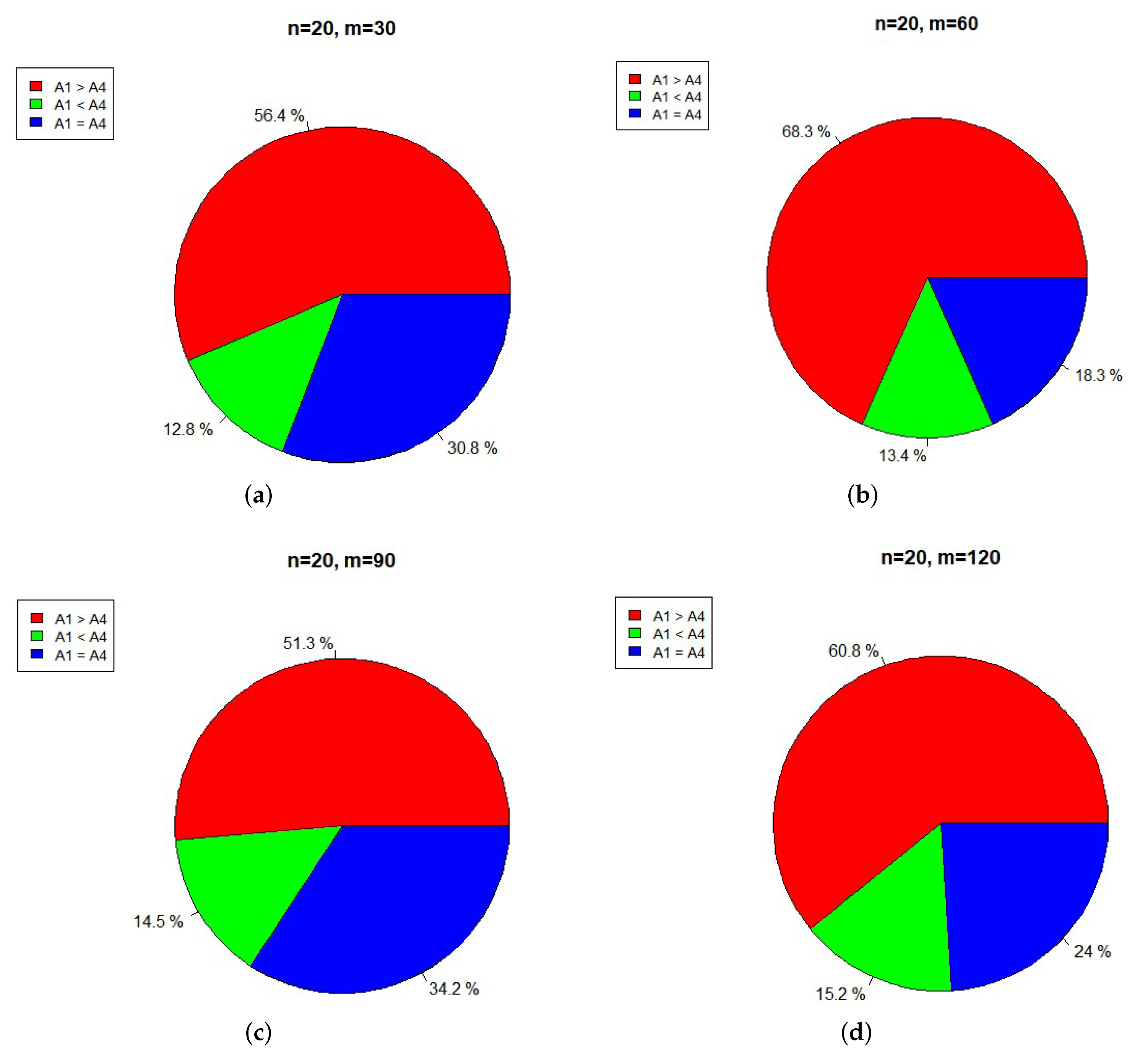
Figure 5 compares the numbers of traversal steps of Algorithms 1 and 2. From Figure 5 we can see that, with the proportion more than $50\%$, Algorithm 1 takes more traversal steps than Algorithm 2 does. In Figure 5, m represents the number of data points in data matrix X; n represents the dimension of data points in data matrix X. “$A1>A4$” means Algorithm 1 takes more steps than Algorithm 2 does. “$A1<A4$” means Algorithm 1 takes less steps than Algorithm 2 does. “$A1=A4$” means Algorithm 1 takes equal steps to Algorithm 2. For each pair $(m,n)$, we run Algorithms 1 and 2 with 100 random data matrices $X_{m\times n}\sim N(\mathbf{0},diag\left(10\right))$. If Algorithms 1 and 2 correctly terminate, then record the number of traversal steps that Algorithms 1 and 2 respectively take.

6. Discussions

Recall that our main focus is the main question: for a given data set X in the tropical projective torus, how to find a tropical polytope $\mathcal{C}$, such that the projection of a Fermat-Weber point of X on $\mathcal{C}$ is a Fermat-Weber point of the projection of X on $\mathcal{C}$? Table 1 and Table 2 shown in Section 5 indicates that Algorithms 1 and 2 can answer the main question with a high success rate, while the success rate of randomly choosing tropical triangles is much lower. For instance, the average success rate of these algorithms in Table 2 is $70.69\%$, and the average success rate of the randomly choosing method in Table 1 is only $6.31\%$. Table 3 shows that the success rate of these two algorithms is stable while the variance is changing with a large range. Compared to Algorithm 1, the advantage of Algorithm 2 is that, Algorithm 2 needs much less computational time, while Algorithm 2 has the same success rate with Algorithm 1 (see Table 4). Figure 5 shows a possible reason for Algorithm 2 being faster: Algorithm 2 usually takes less traversal steps than Algorithm 1 does.

As what has been mentioned in Section 1, this study is motivated by the fact that in tropical PCA [8,9], the variance of the projections might not reach the maximum when the mean squared error reaches the minimum. One possible approach for improving the tropical PCA is using only nice tropical polytopes as the principal component. By “nice tropical polytopes”, we mean the projection of a Fermat-Weber point is a Fermat-Weber point of the projections. Here, our work is the first tool for efficiently computing the nice tropical triangles, which is a potential tool for tropical data analysis. For the users interested in tropical data analysis, we provide the software and system information.

• Software: We implement Algorithms 1 and 2 in R (version 4.0.4) [27], where we use the command lp() in the package lpSolve [26] to implement Line 1 in Algorithm 1 and Line 2 in Algorithm 2 for computing a Fermat-Weber point of a data matrix.
  In our experiments, we use the command rmvnorm() in the package Rfast [28] to generate data matrices that obey multivariate normal distribution.
• Hardware and System: We use a 3.6 GHz Intel Core i9-9900K processor (64 GB of RAM) under Windows 10.

7. Conclusions

In this paper, we develop an Algorithm (Algorithm 1) and its improved version (Algorithm 2), such that for a given data set in the tropical projective torus, these algorithms output a tropical triangle, on which the projection of a Fermat-Weber point of the data set is a Fermat-Weber point of the projections. The experiments presented in Section 5 shows that these algorithms are stable and efficient with high success rate.

We want to highlight that the limitation of the algorithms developed in this paper is that the output of the algorithms is only the tropical convex hull of three points, which means the algorithms cannot be applied to calculate higher dimensional tropical polytopes. In addition, it is not guaranteed that the algorithms will always succeed. In the future, we can continue this study in the following directions. First, in order to generalize the algorithms, one has to generalize Theorem 1 to tropical tetrahedrons or higher dimensional tropical polytopes by studying the relative positions between the points and the polytopes in high dimensional tropical projective torus. Second, one possible way to improve the success rate of the algorithms is to traverse all Fermat-Weber points instead of computing a single Fermat-Weber point in Line 2.