A New Method for Time Normalization Based on the Continuous Phase: Application to Neck Kinematics

Abstract

There is growing interest in analyzing human movement data for clinical, sport, and ergonomic applications. Functional Data Analysis (FDA) has emerged as an advanced statistical method for overcoming the shortcomings of traditional analytic methods, because the information about continuous signals can be assessed over time. This paper takes the current literature a step further by presenting a new time scale normalization method, based on the Hilbert transform, for the analysis of functional data and the assessment of the effect on the variability of human movement waveforms. Furthermore, a quantitative comparison of well-known methods for normalizing datasets of temporal biomechanical waveforms using functional data is carried out, including the linear normalization method and nonlinear registration methods of functional data. This is done using an exhaustive database of human neck flexion-extension movements, which encompasses 423 complete cycles of 31 healthy subjects measured in two trials of the experiment on different days. The results show the advantages of the novel method compared to existing techniques in terms of computational cost and the effectiveness of time-scale normalization on the phase differences of curves and on the amplitude of means, which are assessed by Root Mean Square (RMS) values of functional means of angles, angular velocities, and angular accelerations. Additionally, the confidence intervals are obtained through a bootstrapping process.

1. Introduction

In recent years, the application of nonlinear techniques and advanced statistical methods has received increasing attention for biomechanical analyses. Examples of such biomechanical applications include gait analysis, sit-to-stand movement, sport movements, rehabilitation therapies, and clinical applications, to name but a few (e.g., [1,2,3]). Nowadays, it is easy to collect large amounts of kinematic or dynamic data with motion analysis equipment and labs. In this regard, human movement analysis entails the use of time series of data such as joint angles, velocities, accelerations, forces and moments, mechanical power, landmark positions, etc.

These movement curves may present variations in amplitudes and temporal patterns (phase differences) for different subjects or experimental trials [4,5]. This variability may lead to the statistical cancellation effect related to the aggregation of data [6]. Therefore, the main characteristics of each individual pattern may be hidden when obtaining averaged patterns. Then, the analysis of such data requires some time-scale normalization so that observational curves are comparable. This normalization is intended to match the duration of different registrations, preserve the main features of individual patterns, and reduce variability in the timing of significant events [7].

The most widely used method to normalize time scales in clinical and biomechanical applications is linear normalization, which converts them into a percentage of the duration of the movement analyzed [8]. It is a simple method and can provide good results in many applications [1]. However, it presents some problems that must be considered. On the one hand, it depends on a good estimate of the initial and final moments of the movement, which is not always evident [9]. On the other hand, it implicitly assumes that the duration of the different phases of the movement is scaled to the total duration of the movement. In [7], it is shown that this is not always true, which has important consequences for reducing variability. In fact, it is possible that linear normalization not only does not reduce temporal variability, but actually increases it in cases where there is not a high correlation between the duration of the events and the total duration of the movement.

In the FDA context, other, much more efficient strategies have been developed to reduce phase variability through different nonlinear registration procedures, as reviewed in [10]. Nonlinear time-scale normalization techniques include landmark registration [11], the sequence of states method [12], dynamic time warping [8,13], and curve registration based on correlation criteria [1,9,14] or on the Fisher–Rao Riemannian metric and square-root velocity function (SRVF) [15,16]. Function registration methods could virtually eliminate all phase variability so that the registered curves have the same shape, differing only by the different amplitudes [11,15]. This makes it possible to obtain good estimates of the average curves. However, the temporal information (which in linear normalization is maintained in the lags between curves) does not disappear in this type of rescaling but is maintained in the so-called time warping functions. These functions represent the relationship between the modified time as a function of real time and make it possible to analyze when the movement develops faster or slower than the reference motion.

Despite the attractiveness of these methods, they are not exempt from certain practical limitations. First, their effectiveness in reducing variability depends on the type and characteristics of the functions to be recorded. Thus, when applied to motion curves that have many characteristic points (maxima, minima, inflection points), the reduction in variability is much better than when applied to curves without the existence of such points [1]. In addition, the registration process is complex from a mathematical point of view and presents a high computational cost since the curves must be registered one by one with respect to a reference. Moreover, the registration of curves that differ significantly in the amplitude of their inflection points may distort the functions [17], the so-called pinching effect [10], which causes important distortions in the shape of the curves. In practice, this is equivalent to introducing discontinuities or sudden changes in the warping functions, which is not consistent with the continuous nature of the speed of execution of a movement.

Another drawback of these recording methods is that they are based on the comparison of each curve with a reference standard, usually a mean. This means that they are based on the geometric similarity between pairs of curves, without considering the dynamic nature of the phenomenon they represent, the relationships between the variables and their derivatives. In fact, the results of the registration process can change depending on the order of the derivative used, which is not very consistent from a physical point of view.

This paper presents a novel time-scale normalization method, based on the Hilbert transform (HT), for analyzing functional data and assessing the effect on variability of human movement registrations. This method involves calculating the instantaneous phase of a cyclical movement, which is a concept widely used in nonlinear dynamics. The dynamics of movement are described in terms of the relationships between the variables defining the position of the system and their derivatives, represented in the phase space. Unlike nonlinear recording methods, which are based on comparing each curve with a reference [10], the proposed method exclusively uses the information contained in the curve to be adjusted, providing a generalized phase that varies between 0° and 360° during the execution of a cyclical movement. In this way, it provides a common scale of intrinsic representation of each movement with a mechanical meaning.

Despite its widespread use for describing phases of motor coordination [18], as far as we know, it has never been used as an alternative to time-scale normalization for reducing the variability associated with phase differences. Hence, neither its effectiveness nor its results when normalizing different types of periodic movements have been described. Therefore, a quantitative comparison is made between the proposed method and the two most widely used methods in the field of biomechanics: linear normalization and continuous registration based on correlations [1,9,14]. For this, a comprehensive database of flexion-extension movements of the human neck will be used. The results show the usefulness of the proposed method relative to the current techniques in the literature.

The rest of the paper is organized as follows. Section 2 introduces the materials and methods needed to compare the time-scale normalization methods applied to a human movement database. The data structure is explained in Section 3, while Section 4 presents and discusses the results. Finally, Section 5 draws conclusions from this research.

2. Materials and Methods

A database with flexion-extension movements of the neck will be used to assess the effectiveness of the method. Three normalization procedures have been compared: (a) Linear normalization of the time scale, which is the technique widely used in biomechanical applications; (b) A nonlinear registration method based on correlations; and (c) The method based on the instantaneous phase obtained by the Hilbert transform.

As a nonlinear registration method, we have chosen the one proposed in [9,17]. Although there are more recent alternatives, such as SRVF-based methods [15,16], we have chosen this nonlinear registration method as it is the most widely used in the context of human movement analysis. Since the state of motion of a dynamic system is defined by position and velocity, we have considered two nonlinear registration methods: (b1) using position curves (angles); and (b2) using velocity curves. The characteristics of each of the normalization methods are described below.

2.1. Linear Normalization Method (Scale 0–100%)

Let us consider a set with N temporal functions $x_i\left(t\right)$ representing a position variable associated with a cyclical movement, in our case, the angle of flexion-extension of the neck.

Each curve i can be expressed as a series of values $x_{ij}$, at times $t_{ij}$ sampled in the interval of duration of the movement, $T_i$. All curves are assumed to start at time t = 0, although the durations $T_i$ are different.

$$x_{ij} = x_i\left(t_{ij}\right); i = 1, 2, \dots , N; j = 1, 2, \dots , M_i; t_{i1} = 0; t_{i{M}_i} = T_i$$

(1)

where $M_i$ is the number of samples of the i-th curve. Note that the curves can be sampled at different time intervals ($t_{ij}$ can be different from $t_{kj}$).

The normalization of the time scale from 0 to 100% of the execution time of the movement is performed through a linear transformation, in which the percentage of execution of the movement is calculated with respect to the total duration of the experiment (100% of execution of the movement cycle) for each instant of time. Therefore, the normalized time scale $tn$ is obtained by means of Equation (2).

$$t_{ij}^n = \frac{t_{ij}}{T_i}·100; t_{ij}^n\in \left[0, 100\right]$$

(2)

From the normalized times, the corresponding normalized functions over time, $x^n(t^n)$ are calculated as:

$$x_i^n(t_{ij}^n) = x_i\left(t_{ij}\right)$$

(3)

All $t_{ij}^n$ are defined in the same interval, [0, 100], although they do not necessarily correspond to the same instants. For the normalized curves to be comparable, the last step is to interpolate the $x_i^n$ curves to express them all in the same equispaced values of $t^n$, with a step equal to 1%. In this way, all functions are defined in the same normalized instants [0, 1, 2 … 100]% of the duration of the movement.

It is important to note that linear normalization is performed independently for each $x_i\left(t\right)$ curve. No comparison is made between the curves of the set since each curve only uses a single parameter, the duration of that movement, $T_i$. Note also that the normalized time is the same for the function $x_i\left(t\right)$ or for its first and second derivatives.

2.2. Nonlinear Registration Method of Functional Data Using Angles or Velocities

The procedure used for registering position or velocity curves is described in [9]. Let us consider the set of N curves to be registered, $x_i\left(t\right),$ that correspond to the position variables or their derivatives. In this work, flexion-extension angles and their first derivative have been used. We will assume that all the curves are defined in the same time interval [0, T], which implies a previous process of linear normalization of time.

The registered curves are a new set of curves $x_i^{\ast }\left(t\right) = x_i\left(h_i\left(t\right)\right)$, where $h_i\left(t\right)$ functions are a nonlinear transformation of the time scale called a warping function. The warping functions must minimize the phase differences between each curve, $x_i^{\ast }\left(t\right)$, and a reference curve $x_o\left(t\right)$. Note that the nonlinear registration process involves comparing each curve in the set with a reference curve, usually the functional mean of the set, $\overline{x}\left(t\right)$ [17]:

$$x_0\left(t\right) = \overline{x}\left(t\right) = \frac{1}{N}{{\displaystyle \sum }}_{i=1}^N{x}_i\left(t\right)$$

(4)

Since functional averages are affected by the cancellation effect, the adjustment process cannot be done all at once, but rather, through a Procrustes process, as discussed later.

The calculation of $h_i\left(t\right)$ is associated with an optimization process where the variability associated with the amplitude must be maximized, and the variability associated with the phase differences must be minimized. This cannot be done directly on the differences between a curve before and after the registration procedure because in such a case, the method tries to compress the regions where amplitudes differ [17]. It distorts the shape and temporal patterns of functions since a function minimizes the variability and perfectly fits another function, except in the vicinity of the maxima and minima. Another more rigorous method has been used to overcome this shortcoming, based on some ideas from principal component analysis (PCA) [9]. The method used is based on minimizing the second eigenvalue of the cross-product matrix $L$ given by Equation (5).

$$L = \left(\begin{array}{cc}{\displaystyle \int }{x}_0^2\left(t\right)dt& {\displaystyle \int }{x}_0\left(t\right)x_i\left(h_i\left(t\right)\right)dt\\ {\displaystyle \int }{x}_0\left(t\right)x_i\left(h_i\left(t\right)\right)dt & {\displaystyle \int }{x}_i^2\left(t\right)dt\end{array}\right)$$

(5)

This matrix is symmetric, and hence, has two real eigenvalues. The largest of them (${\mu }_1$) corresponds to the variance associated with the amplitude differences, while the second (${\mu }_2$) is associated with the phase differences [17]. Therefore, the best fit between $x_0\left(t\right)$ and $x_i\left(t\right)$ is obtained by means of a function $h_i\left(t\right)$ that minimizes the smallest eigenvalue of the matrix. In practice, this value is not used directly but rather its logarithm. So that the objective function to optimize is $F\left(h_i\right) = \log {\mu }_2$.

The warping functions are required to have an integrable second derivative and also to be strictly increasing. As explained in [17], such functions can be described by the homogeneous linear differential Equation (6)

$$D^2{h}_i = w_{i}D{h}_i$$

(6)

where $D$ and $D^2$ denote the first and second derivatives, respectively, and $w_i\left(t\right)$ is any unconstrained function. This equation is also subject to the constraints $h\left(0\right) = 0$ and $h\left(T\right) = T$, which makes it possible to obtain its solution as presented in [9].

Then Equation (6) has the solution

$$h_i\left(t\right) = C_i{{\displaystyle \int }}_0^t\exp ({{\displaystyle \int }}_0^u{w}_i\left(v\right)dv)du$$

(7)

where $C_i = T/[{{\displaystyle \int }}_o^{T}exp\{{{\displaystyle \int }}_0^u{w}_i\left(v\right)dv\}du]$.

Note that Equation (6) and the function $w_i\left(t\right)$ are introduced to calculate the function $h_i$ that minimizes $F\left(h_i\right) = \log {\mu }_2$, under the constraint that it is strictly increasing. In this way, the optimization problem is carried out through $w_i$.

As mentioned before, the nonlinear registration is performed by comparing each function $x_i\left(t\right)$ with the functional mean of the set, $x_0\left(t\right)$. Since the original functions are not aligned, the mean $x_0$ will be affected by the cancellation process, which can distort the results. A Procrustes method is used to avoid this. It consists of an iterative process in which the registration of the set of curves is repeated several times so that a new $x_0$ is obtained in each iteration, serving as a reference for the next registration. The process converges in a few iterations. In this work, we have used three iterations [9].

The registration process involves making a comparison of the reference curve with each of the sets, which implies the nonlinear optimization of N functions $h_i\left(t\right)$. Also, it must be repeated three times in the Procrustes process, which means performing 3N nonlinear optimizations. This involves a much longer computation time than methods where curves are not compared, such as nonlinear normalization or the Hilbert transform-based method described in the next subsection.

2.3. Nonlinear Hilbert Transform (HT) Method

The idea of obtaining an instantaneous phase of a movement comes from the description of the dynamics of an oscillatory system through phase portraits, in which velocity versus position is represented. In the case of harmonic motion of amplitude A and angular frequency $w$, that diagram is a centered ellipse. If the motion begins at the point of maximum elongation, then the $x$ and $y$ components are: $x = A\cos \left(wt\right); y = v = -Aw\sin \left(wt\right)$. Normalizing by the amplitudes, the instantaneous phase can be calculated as:

$$\varphi \left(t\right) = \arctan \left(\frac{-y}{wx}\right) = wt$$

(8)

This approach can be extended to the calculation of the phase in other cyclical movements, in which case a phase is obtained that does not depend linearly on time, that is, with a variable angular frequency, $w\left(t\right)$. This approach has been widely used in movement analysis to describe the coordination between the movements of different joints. It is very consistent when it comes to quasi-harmonic periodic signals but offers debatable results in other cases; for example, when there are several relative maxima or minima in each cycle, which lead to a change of direction of the phase velocity. Therefore, we propose to use the Hilbert transform (HT) as a way of obtaining a smoothed phase diagram in the analysis of human movements. HT has been widely used in different engineering applications, mainly in signal analysis [19]. However, its use in Biomechanics is scarce and has been related to the study of motor coordination rather than normalizing the phase of the curves associated with human movement [18,20].

Given that the HT is applied to each curve separately, regardless of the rest of the set, in this section, we will dispense with the subscripts, explaining how the HT of an individual curve is obtained.

The HT is a specific linear operator that takes a function, $x\left(t\right)$, of a real variable and provides another function of a real variable, $\widehat{x}\left(t\right) = H\left[x\left(t\right)\right]$. This linear operator is given by convolution with the function $1/\left(\pi t\right)$, i.e., the HT of $x$ can be considered as the convolution of $x\left(t\right)$ with the function $g\left(t\right) = 1/\left(\pi t\right)$, which is referred to as the Cauchy kernel. Since $1/t$ is not integrable across $t = 0$, the integral defining the convolution does not always converge. Therefore, the HT is defined using the Cauchy principal value (P). The HT of a function $x\left(t\right)$ is traditionally defined by means of an improper integral (Equation (9)), provided this integral exists as a principal value.

$$\widehat{x}\left(t\right) = H\left[x\left(t\right)\right] = \frac{1}{\pi }P{{\displaystyle \int }}_{-\infty }^{+\infty }x\left(\tau \right)\ast \frac{1}{t-\tau }d\tau$$

(9)

The Hilbert transform allows the transformation of any real signal into a complex, analytic signal $X\left(t\right)$ defined as

$$X\left(t\right) = x\left(t\right) + j\widehat{x}\left(t\right) = A\left(t\right)e^{j\varphi \left(t\right)}$$

(10)

From Equation (10), the instantaneous phase, $\varphi \left(t\right)$, is defined as

$$\varphi \left(t\right) = \arctan \left(\frac{\widehat{x}\left(t\right)}{x\left(t\right)}\right)$$

(11)

Subsequently, the derivative of $\varphi$(t) is the angular frequency, ω(t) = d$\varphi /dt$, which can be interpreted as the instantaneous velocity of the execution of the movement, in terms of phase velocity. In this work, the HT has been computed by means of the MATLAB function “hilbert.m”. This function returns the analytic signal $X\left(t\right)$ in Equation (10).

The HT is not directly applied to the $x\left(t\right)$ functions, but rather they must be centered to avoid distortions in the phase associated with a continuous offset between functions. The centering of each curve is calculated by subtracting a certain parameter from each curve, as shown in Equation (12).

$$x_{centered}\left(t\right) = x\left(t\right) - \frac{\left[\max \left(x\left(t\right)\right)+\min \left(x\left(t\right)\right)\right]}{2}$$

(12)

2.4. Procedure to Measure the Effectiveness of Each Time-Scale Normalization Method

Four comparisons are carried out among different normalization methods of functions. The first one is based on the comparison of warping functions, $h_i\left(t\right)$ for nonlinear registration or $\varphi \left(t\right)$ in the case of HT. We analyzed their continuity, absence of singularities, and coherence with the dynamics of the movement. It is assumed that the warping functions must be smooth and must not present discontinuities.

The second one uses the amplitude of the functional mean obtained with each type of normalization. It is assumed that higher RMS (root mean square) values are associated with better control of phase differences by avoiding the cancellation effect associated with the lags between curves, which translates into a flattening of the maxima and minima. There is only one data set and, consequently, a single mean function for the angle, velocity, and acceleration. In order to test the significance of the differences in the RMS values of the means obtained with the different normalization methods, a bootstrap method has been followed to establish the confidence intervals of the means for α = 0.05 (those shown in the

Table 1. Root Mean Square (RMS) values of the functional means of angles, angular velocities, and angular accelerations as a function of the time-scale normalization method. In parentheses, the 95% confidence interval.

Function	Linear Normalization	Registration Using Angles	Registration Using Velocities	Hilbert Transform
RMS value of the functional mean of the angle (°)	45.8 [42.8, 48.6]	45.8 [42.8, 48.6]	45.4 [42.3, 48.3]	45.3 [43.6, 46.9]
RMS value of the functional mean of the angular velocity (°/s)	89.7 * [81.9, 97.1]	94.2 [86.3, 102.1]	95.0 [87.3, 103.5]	95.6 [91.5, 99.8]
RMS value of the functional mean of the angular acceleration (°/s2)	203.8 ** [187.5, 221.6]	218.4 [202.2, 235.6]	237.0 *** [222.6, 253.0]	219.3 [210.4, 228.9]

Differences with respect to the HT method: * p < 0.05; ** p < 0.01; *** p < 0.005 The significance levels have been obtained from confidence intervals of 0.005, 0.01, and 0.05, calculated through a bootstrapping process.

), but also for α = 0.01 and α = 0.005, which allows us to estimate whether the differences correspond to p < 0.05, p < 0.01, or p < 0.005, respectively [21].

Thirdly, the phase differences between the individual signals and the ensemble mean signal for each normalization method are measured directly using the procedure described in [17]. It consists of defining two time series, x and $y$, which are considered as vectors of an n-dimensional space so that the angle they form is obtained through Equation (13).

$$\cos \theta = \frac{dot\left(x,y\right)}{norm\left(x\right)·norm\left(y\right)}$$

(13)

where $dot\left(x,y\right)$ is the dot product of x and y (Euclidean inner product) and $norm\left(x\right)$ is the L² norm ($norm\left(x\right) = \sqrt{dot\left(x,x\right)}$).

When this procedure is applied to harmonic functions, it results in the lag between them. In other types of signals, it is a measure of the phase difference. When the $\cos \theta$ is 1, then the functions are in phase. On the contrary, a null value of (13) represents two orthogonal functions with a phase shift of 90°.

Subsequently, the mean of each variable is calculated for each normalization method, and the phase difference of each curve with respect to that mean is calculated. The discrepancies are generally small since the curves are approximately harmonic, beginning and ending in the same place. This leads to clearly asymmetric distributions, in which the differences are analyzed using the Friedman test [22].

Finally, we measured the computational cost of the four normalization procedures on the same computer.

3. Application to a Case Study. Data Structure

A quantitative comparison of different methods for normalizing temporal patterns using registration of functional data is performed based on an exhaustive database of neck flexion-extension movements. The database corresponds to 31 subjects, each of whom was measured in two different trials, executing between 7 and 10 complete cycles of neck flexion-extension movements in each trial. The subjects were informed regarding the aim of the experiment, and they signed the corresponding informed consent.

The Kinescan/IBV^® v.5.5 photogrammetry system was used to record and analyze the motion data captured using a helmet with eight reflective markers, according to the procedure described in [23]. The movement was recorded at 200 frames per second. The experimental setup is shown in Figure 1. The flexion-extension angles were measured and the angular velocities and accelerations were calculated using the procedures described in [23,24].

The start and end points of each extension-flexion cycle are determined using the procedure described in [23], so that each cycle begins at a point of zero velocity and minimum angle and ends at the next minimum angle. Obviously, each cycle has a different duration due to the differences between subjects and within each subject in different repetitions.

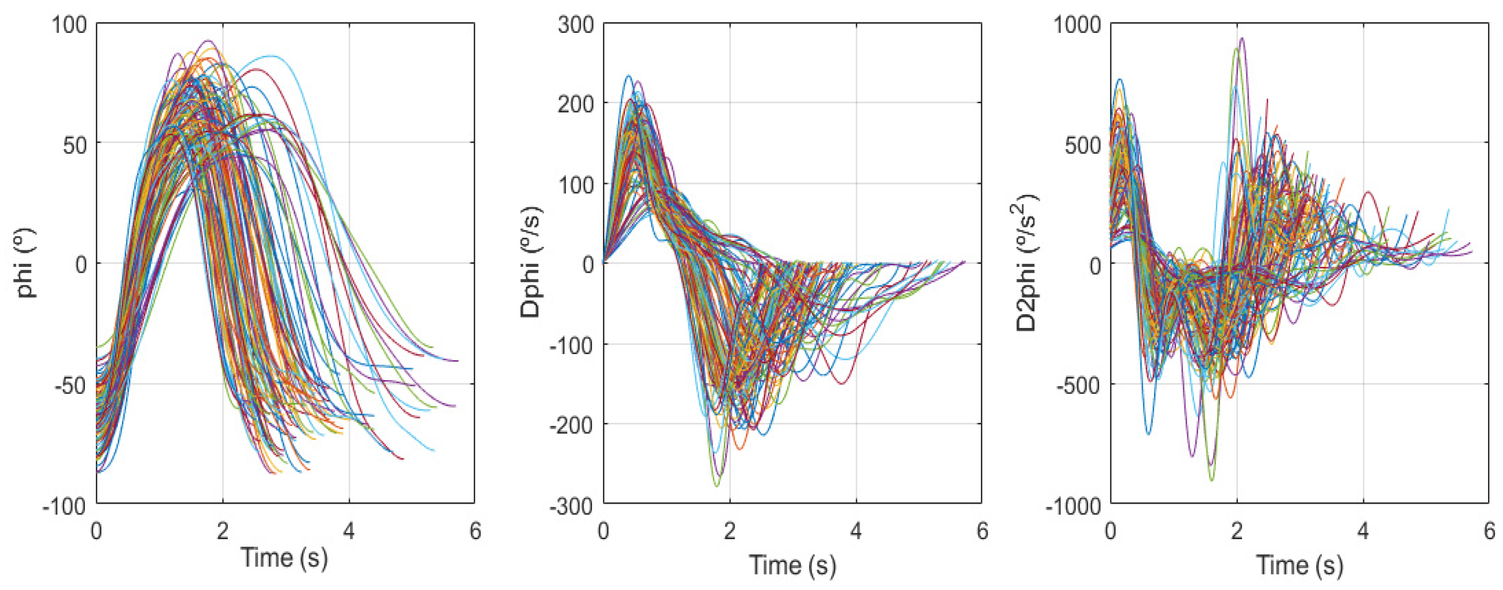
Consequently, the database is made up of matrices with a size of 1254 × 423 for the variables related to angles (phi), angular velocities (Dphi), angular accelerations (D2phi), and absolute times sampled at a frequency of 200 Hz. That is, matrices with dimensions equal to the length required for the longest registration.

The normalized curves are expressed in two different formats. On the one hand, in the case of linear normalization and nonlinear registration (from angles or velocities), the normalized curves are represented with 101 observations, on a time scale between 0 and 1 for each cycle, at intervals of 0.01 steps. On the other hand, for recording using the phase obtained from the Hilbert transform, the X-axis uses a scale between 0 and 360°, at 1° intervals. However, in the figures presented in the following sections, the scale for the continuous phase is divided by 360 in order to compare the results with those obtained with the normalized times, so the scale of the X-axis goes from 0 to 1 in all cases.

As a result, the database is made up of 423 complete cycles, which have been used to perform the quantitative comparison of the different methods.

The database encompasses the following variables:

• philn: angle with linearly normalized time.
• Dphiln: angular velocity with linearly normalized time.
• D2philn: angular acceleration with linearly normalized time.
• phiR0: angle with time registered using angle curves.
• DphiR0: angular velocity with time registered using angle curves.
• D2phiR0: angular acceleration with time registered using angle curves.
• phiR1: angle with time registered using the angular velocity curves.
• DphiR1: angular velocity with time registered using the angular velocity curves.
• D2phiR1: angular acceleration with time registered using the angular velocity curves.
• phiH: angle using the phase obtained with the Hilbert transform (HT).
• DphiH: angular velocity using the phase obtained with the Hilbert transform.
• D2phiH: angular acceleration using the phase obtained with the Hilbert transform.

4. Results and Discussion

Figure 2 shows the absolute time-scale curves for angles (phi), velocities (Dphi), and accelerations (D2phi), which exhibit a large dispersion and show the need for normalizing the temporal patterns.

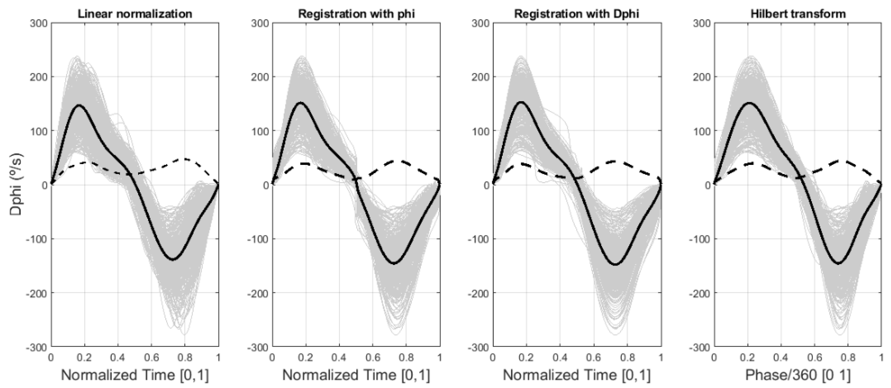
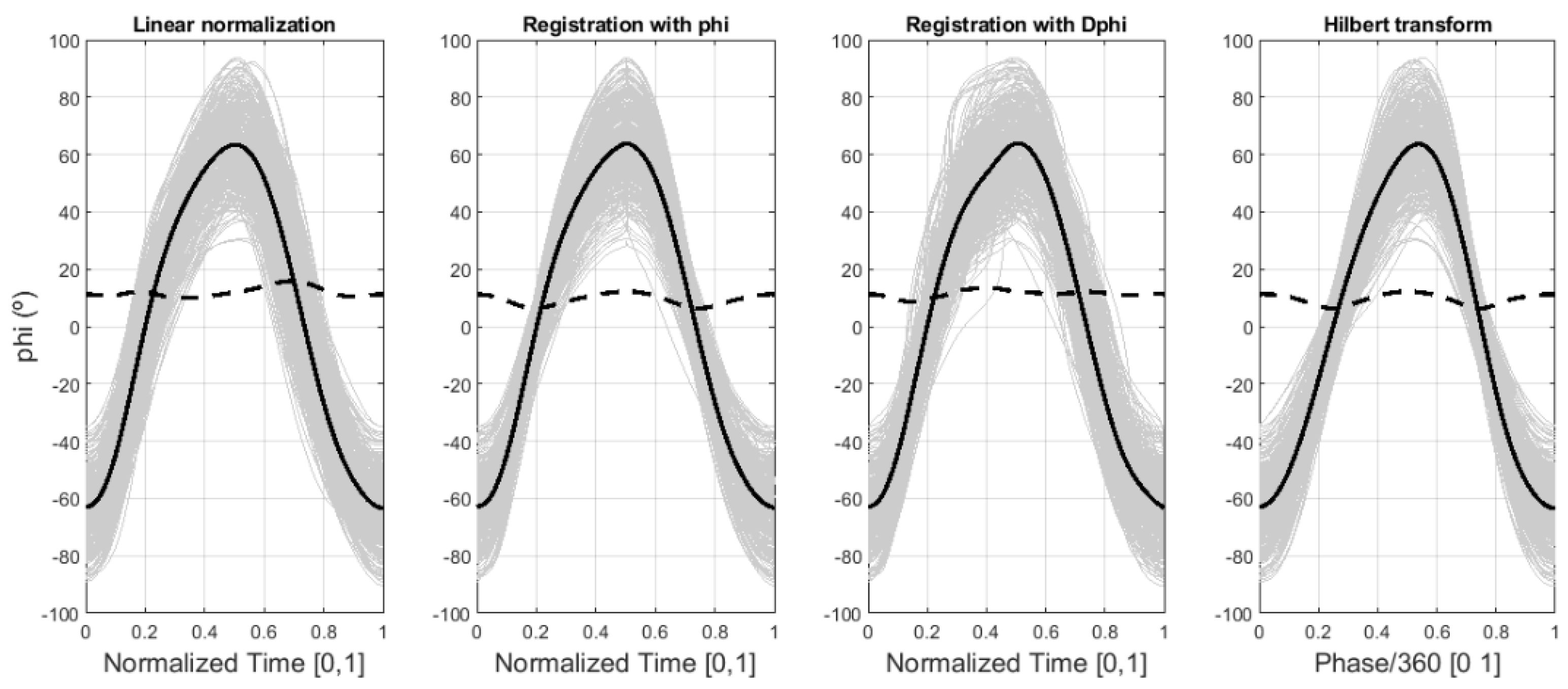
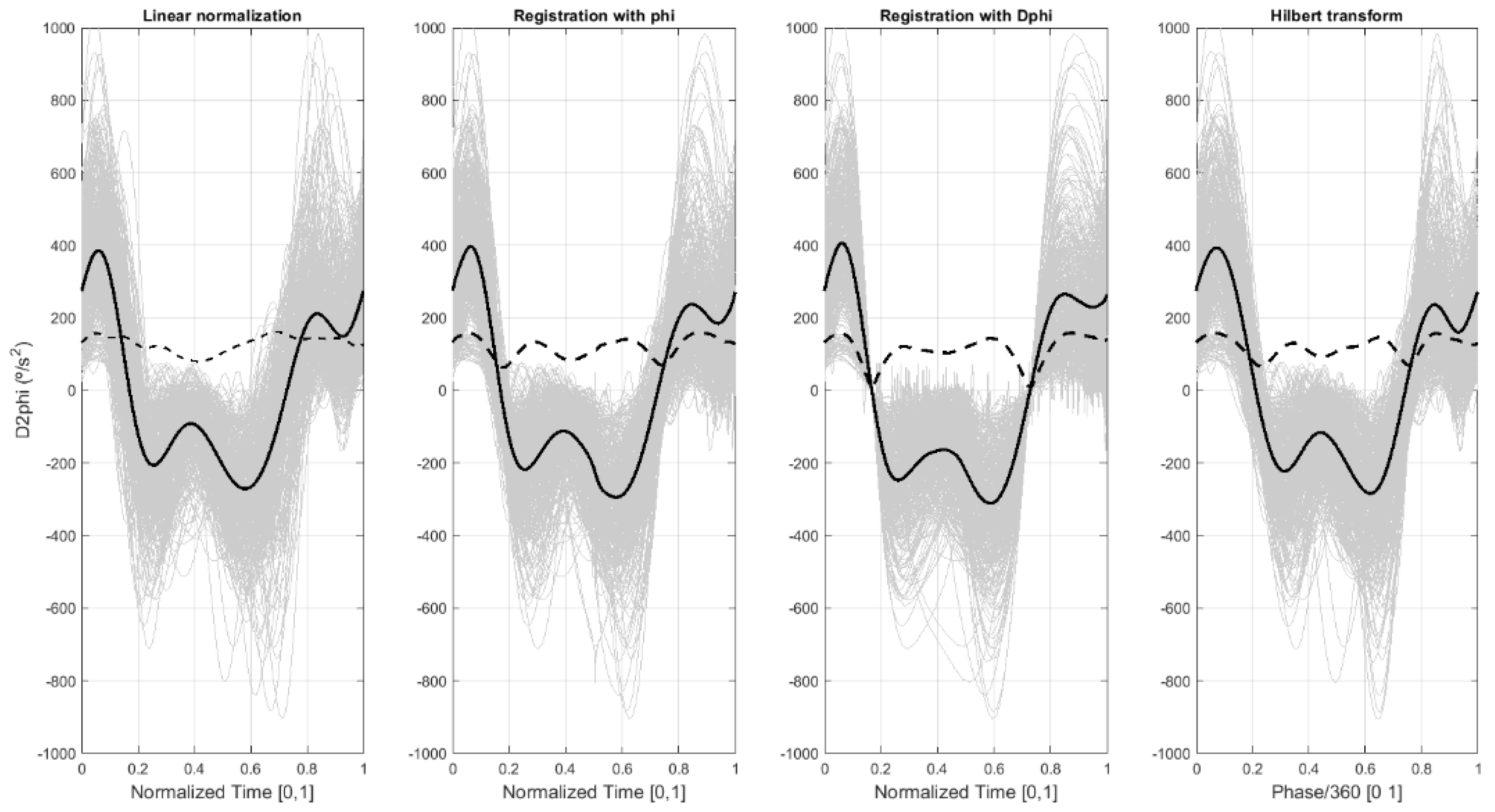
Figure 3 presents the normalized angle (phi) curves obtained by means of the four normalization methods compared, together with their functional means (solid black line) and functional standard deviations (dashed black line). Figure 4 and Figure 5 do the same for the normalized velocities (Dphi) and accelerations (D2phi), respectively. These figures also show the large amplitude dispersion of the human neck flexion-extension movements measured for 31 healthy subjects in the two trials of the experiment. Note that for this figure and the following ones, the phase is divided by 360, so the X-axis scale ranges from 0 to 1, thus making the results comparable among the four methods.

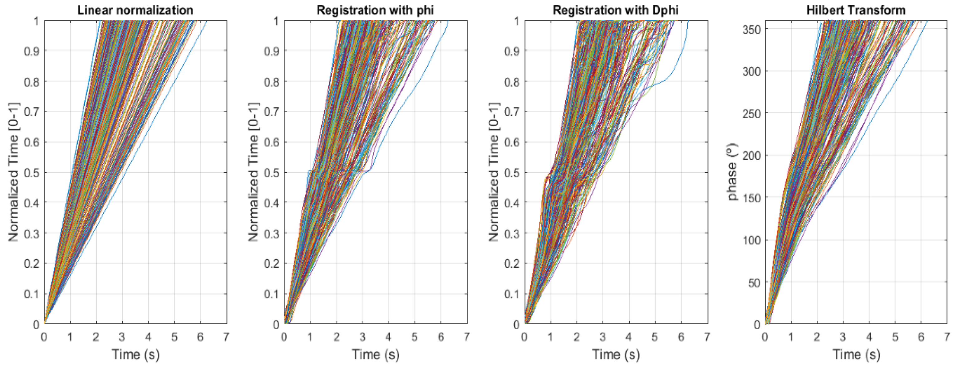
Figure 6 illustrates the time warping functions for the four compared methods, which represent the relationship between the normalized and the absolute times. Based on the results, several conclusions can be drawn:

• On the one hand, for the linear normalization method, the warping functions are straight lines, as expected. On the other hand, for the nonlinear methods (registration of functions and HT method), nonlinear warping functions are achieved.
• The registration of functions method leads to different warping function curves when angles or velocities are used as the registration source.
• Registration using angles tends to present significant variations in the time recorded in the vicinity of the central zone (which corresponds to the maximum angle). This can be observed around the time of 0.5 s in the normalized time (Y-axis of Figure 6), where there are curves in which the absolute time advances but the recorded time does not. This distortion in the shape of the warping functions can appear when the differences in amplitude are optimized at the expense of unnatural alterations over time [17]. In practice, this is equivalent to introducing discontinuities or sudden changes in the warping functions, which is not consistent with the continuous nature of the speed of execution of human neck movements.
• Registration using velocities also leads to distortions in the warping function curves, although to a lesser extent.
• Consequently, these two characteristics (i.e., obtaining different results according to the order of the derivative used for registration; and the existence of singularities in the warping functions) reveal that although it is an effective technique, it is purely geometric and unrelated to the dynamics of the functions.
• The HT method provides nonlinear curves, but they are smoother and without sudden changes. Hence, the differences between the normalized and the absolute times are not significant but have consequences for the mean, phase differences, and dispersion values. Note that we are analyzing a cyclical movement similar to a harmonic one.

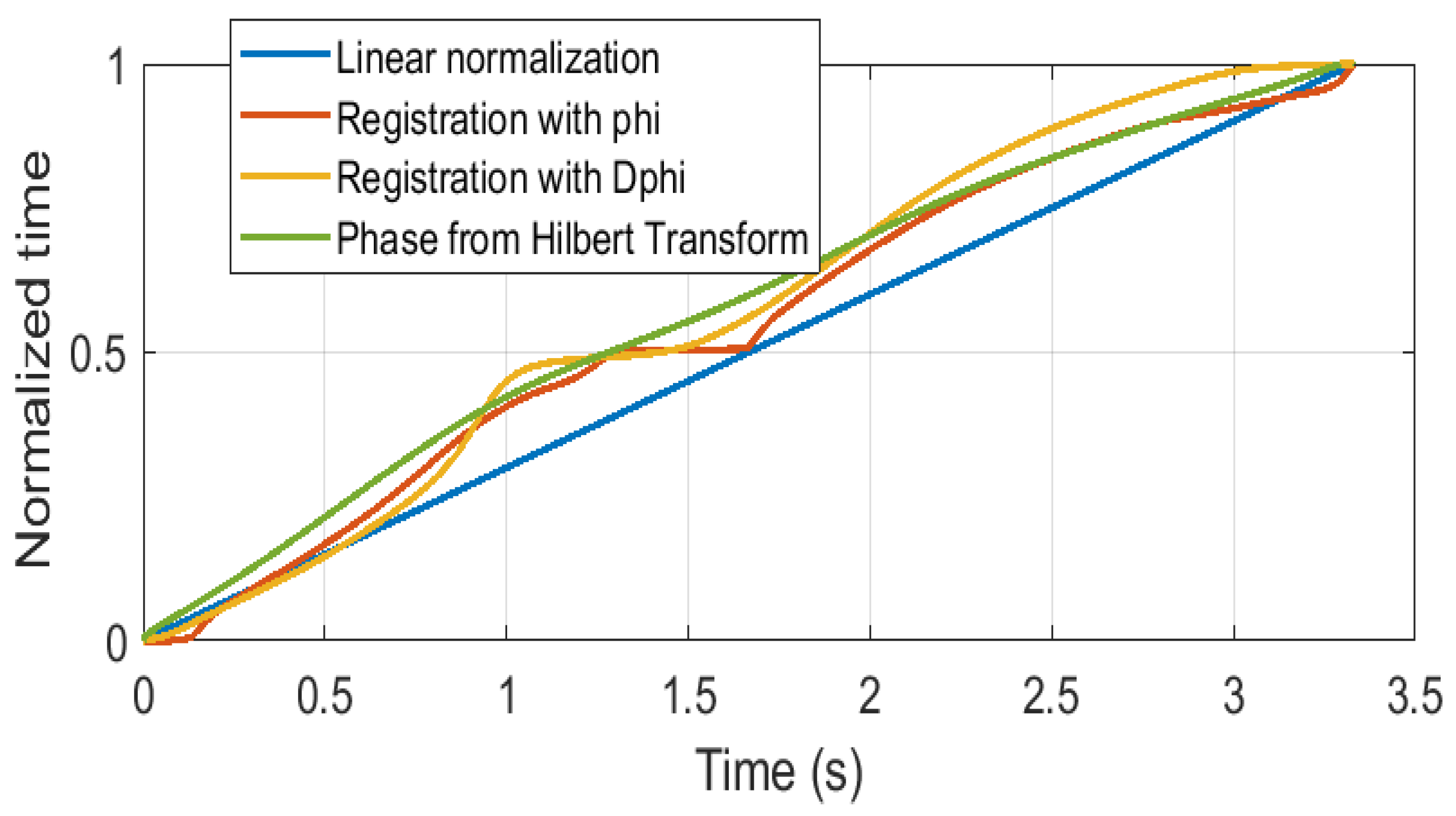
Such differences can be better appreciated in Figure 7, which compares the warping functions of the four methods for a certain registration curve (register number #345). Again, it can be observed that the HT method provides a smooth and nonlinear recording, while the registration of functions methods using either angles or velocities present singularities and give rise to different curves. It is worth mentioning that although the R0 and R1 warping functions are quite similar in this case, in other cases, they may differ substantially.

4.1. Comparison of the Effect of Time-Scale Normalization on the Amplitude of the Means

Table 1 presents the Root Mean Square (RMS) values of the functional means of angles, angular velocities, and angular accelerations for the time-scale normalization methods compared. The results illustrate that when comparing the different time scale normalization methods, there is hardly any difference for angles because the phase differences are small and do not affect the mean or the RMS values.

However, for the angular velocities, the HT method improves the results provided by the linear normalization method since it leads to 6.6% higher RMS values. Conversely, there are no significant differences regarding the RMS values provided by the nonlinear registration method.

With regard to angular accelerations, HT-based normalization is significantly better than the linear normalization method (a 7.6% higher RMS value) and similar to the nonlinear registration method using angles. However, the RMS values obtained when using velocity curves outperform those provided by the HT method. In fact, an improvement of 8% is achieved.

4.2. Comparison of the Effect of Time-Scale Normalization on the Phase Difference

Table 2. Distribution of the phase difference between the individual curves of angles (phi), angular velocities (Dphi), and angular accelerations (D2phi), and their corresponding functional means, for each time-scale normalization method. The median and interquartile range are measured in degrees. The level of significance of the comparison of each normalization method with the Hilbert transform, using Friedman’s test, is presented in brackets.

Variable	Linear Normalization Median (iqr) [p-Value]	Registration Using Angles Median (IQR) [p-Value]	Registration Using Velocities Median (IQR) [p-Value]	Hilbert Transform Median (IQR)
phi	10.7 (8.0) [0.0000]	4.2 (7.5) [0.0000]	9.1 (7.1) [0.0000]	5.5 (6.5)
Dphi	11.0 (6.7) [0.0000]	7.0 (3.4) [0.0000]	4.5 (5.4) [0.000]	7.8 (4.3)
D2phi	23.5 (12.9) [0.0000]	19.4 (8.9) [0.05779]	15.4 (5.7) [0.0000]	19.3 (10.0)

shows the medians and interquartile ranges (IQR) of the phase difference for each time-scale normalization method. IQR is used as a measure of the statistical dispersion, which is equal to the difference between the 75th and 25th percentiles or between the upper and lower quartiles.

The worst results for the three variables are obtained for linear normalization. This is because this process leads to higher phase differences for such variables, which are represented by the median and interquartile range (Table 2). Furthermore, the phase difference presents much worse results for velocities, and even more so for accelerations. This calls into question the usefulness of linear normalization for an adequate representation of the kinematics and dynamics of human movements. Note that we are analyzing a cyclical movement where all cycles start and end at the same values. In contrast, the HT method obtains much better results than the linear normalization method for angles (the phase difference is reduced to almost half). The reductions of the lags in velocities are somewhat smaller but are still important, 29% in the velocities and 18% for the accelerations.

The nonlinear registration method is also clearly better than the linear normalization method, although it provides different results depending on whether position or velocity registration curves are used. Angular curves return the best results with the R0 registration, while the R1 registration, using velocity curves, is better for velocities and accelerations. The fact that the results differ according to the registration curves used for normalization, both in phase differences and in the warping functions, suggests that nonlinear registration is an inconsistent method. That is, the function registration method provides different results for the same data depending on the order of the derivative used in the registration curves. Although this method provides formally suitable results (for both angles and velocities if registration using angles or velocities are used, respectively), it entails a purely geometric adjustment. Therefore, it is questionable that it fulfills the characteristics of the dynamics of the movement. To overcome this drawback [17] proposed to use higher-order derivatives for the registration of functions, assuming that by using more maxima and minima, more temporal information is retained. Unfortunately, this is not true in our case, since the registration using velocities is worse than using angles if we measure the phase angle difference, although better if the phase velocity difference is considered. We have not calculated the registration using accelerations.

Regarding the method of representing kinematic variables as a function of the phase obtained by means of the Hilbert transform, the results exceed those obtained with the linear normalization method in the variables of position, velocity, and acceleration. Nevertheless, the comparison of the Hilbert transform method with the nonlinear registration method leads to somewhat contradictory results. In this sense, the Hilbert transform provides better results than the R1 registration for position and worse for velocity and acceleration curves. When the HT method is compared with the R0 registration, it presents results that are worse for angular curves, slightly worse for velocity curves, and similar for acceleration curves. However, the differences between the HT method and the registration of functions method are considerably smaller than those between HT and the linear normalization method. It is worth mentioning that the HT method involves a lower computational cost than the nonlinear registration method. Furthermore, HT does not alter the dynamic relationships between the angles and their derivatives since the time scale is not changed. Instead, it is replaced by another variable, the phase of the movement, which is related to the relative velocity of execution within the cycle of movement.

As a summary, for the three variables analyzed, the following conclusions can be drawn:

• Phase angle difference (phi): the best method is the registration method using angles. The HT method is much better than linear normalization and nonlinear registration using velocities.
• Angular velocities (Dphi): the smallest lags are obtained with nonlinear registration using velocities. Nonlinear registration using angles and the HT method offer similar values, although slightly better in the former. The worst result is obtained for the linear normalization method.
• Angular accelerations (D2phi): the pattern is repeated for the case of accelerations. That is, the worst method is linear normalization, and the best is registration of functions using velocities. Nonlinear registration using angles and the HT method provide very similar results.

4.3. Comparison of Computational Efficiency

Although the computational cost is not a limiting factor for applying any of the normalization methods, significant differences are appreciated in terms of execution times. The linear normalization method has the lowest computational cost, with an execution time of only 0.21 s. The Hilbert transform method entails a simulation time of 0.61 s (2.9 times higher than linear normalization). Finally, the nonlinear registration method using angles requires a running-time cost of 968.3 s (16.1 min), while registration using velocities takes 1230 s (20.5 min). That is, nonlinear registration reports execution times around 4610.9 and 5857 times higher than the linear normalization method, respectively. As mentioned above, the high computational cost of nonlinear registration methods is due to the fact that in each iteration of the Procrustes process, they must perform a nonlinear optimization for each $h_i$. Linear and HT methods perform normalization only once per curve using fast calculation procedures.

These values reinforce the idea that the HT method provides excellent results with a low computational cost compared to the other time-scale normalization methods.

5. Conclusions

This paper presents a novel method for normalizing human movement patterns using functional data analysis with key applications in the fields of biomechanics and ergonomics. The method is based on the Hilbert transform, and is very useful for the normalization of human movement curves due to its enormous potential in reducing variability among registrations. Furthermore, a quantitative comparison of methods for normalizing time-series data has been carried out based on an exhaustive database of neck flexion-extension movements. It is noteworthy that time-scale normalization methods play a major role in functional averages, since they affect the lag between curves. Moreover, they can alter the shape of the ensemble mean of individual curves and reduce its amplitude. This raises the need to develop appropriate methods to deal with such issues.

The linear normalization method has traditionally been used for reducing phase lags because of its simplicity and low computational cost. However, the results have shown that linear methods do not allow us to fully control phase differences, even in apparently harmonic cyclical movements, such as neck flexion-extension movements. Therefore, the worst of the four methods compared is, by far, linear normalization in terms of reducing phase lags and cancellation effect. The worse behavior of the linear normalization method implies a reduction in the amplitude of the averaged curves, which has been measured through RMS values. Although the differences in angular curves are negligible, they are significant for velocity and acceleration curves. Consequently, the use of linear methods must be avoided.

Several nonlinear registration methods have been proposed in the literature to overcome these drawbacks. However, our results show that these methods can present some problems. Firstly, their results differ depending on the order of the derivative used as the reference for the record. That is, different rescaled times appear for the same dynamic system depending on the order of the derivative of the functions. This does not make much sense from a mechanical point of view, as the position and velocity variables correspond to the same movement, contradicting the assumption that such methods are capable of identifying “system time” from the absolute clock time [10]. In addition, some inconsistencies may arise, such as singularities at certain points, which, although they limit the phase differences, give rise to curves without any physical sense. Finally, nonlinear registration methods are computationally expensive compared to linear or HT methods.

The results have also shown that the proposed method to normalize temporal patterns can improve on the current techniques in the literature in terms of reducing phase differences with good computational efficiency. It consists of replacing the time scale with the instantaneous phase of the movement obtained from the Hilbert transform. We have verified the following advantages of the presented methodology:

• It provides a single result (angle and velocity are used at the same time).
• The results are clearly better than those of the linear time base regarding velocities and accelerations and similar to the nonlinear registration method in terms of velocities. Regarding accelerations, it is similar to registration using angle curves and somewhat worse than registration using velocities.
• From a computational point of view, it is much faster than nonlinear registration by three orders of magnitude.
• It does not give rise to warping functions with singularities, but rather the phase curves are smoother.
• The proposed method uses the information of the movement of each individual curve, obtaining an instantaneous phase with mechanical meaning. Its derivative is an instantaneous angular frequency representing a phase velocity, and it is independent of the curve amplitude.

The results shown here correspond to a relatively harmonic type of cyclical movement, although less harmonic than others described in the literature [1]. To generalize the conclusions on the performance of HT, it would be necessary to compare the methods using other more complex cyclical movements, such as human gait.

On the other hand, we have used the nonlinear registration method proposed in [17], as it is the most widely used in the field of Biomechanics. As indicated above, there are other more recent alternatives, such as those based on SRVF [15], whose application in the field of human movement analysis is limited so far [16], but which should provide better results than those based on correlations.

As further research, the HT method could be applied to movements that are highly sensitive to variability, such as the instantaneous axes of rotation of joints. In addition, the velocity of execution of the movement is currently tackled using parameters such as cadence, frequency of movement, period between cycles, etc., which do not offer continuous information on the instantaneous velocity of execution of the movement. Conversely, this novel normalization technique could lead to new functional assessment systems for analyzing this type of movement through phase velocity and quantifying harmonic motions. Phase velocity could be used for detecting abnormal behaviors associated with acute pain or simulation, which are currently analyzed through other parameters such as the correlation between position and acceleration, jerk, etc. However, these parameters depend on second or third derivatives and are quite sensitive to the derivation method used. We consider that the amplitude of phase velocity is a much simpler indicator for quantifying the deviation between a harmonic movement (with constant phase velocity) and a nonharmonic one (with important oscillations in the phase velocity).