
An Efficient Algorithm for Convex Biclustering


Abstract
:1. Introduction
- We propose an efficient algorithm to solve the convex biclustering model for large-scale N and p. The algorithm is a first-order method with simple subproblems. It only requires calculating the matrix multiplications and simple proximal operators, while the ADMM approaches require matrix inversion.
- Our proposed method does not require as much computation, even when the tuning parameter is large, as the existing approaches do, which means that it is easier to obtain biclustering results simultaneously for several values.
2. Preliminaries
2.1. ADMM and ALM
2.2. Nesterov’s Accelerated Gradient Method
| Algorithm 1 NAGM. |
Input: Lipschitz constant L, initial value , . While (until convergence) do
End while |
2.3. Convex Biclustering
3. The Proposed Method and Theoretical Analysis
3.1. The ALM Formulation
3.2. The Proposed Method
| Algorithm 2 Proposed method. |
Input: Data X, matrices C and D, Lipschitz constant L calculated by (27), penalties and , initial value , , . While (until convergence) do
Output: optimal solution to problem (8), . |
3.3. Lipschitz Constant and Convergence Rate
4. Experiments
4.1. Artificial Data Analysis
- Relative error:
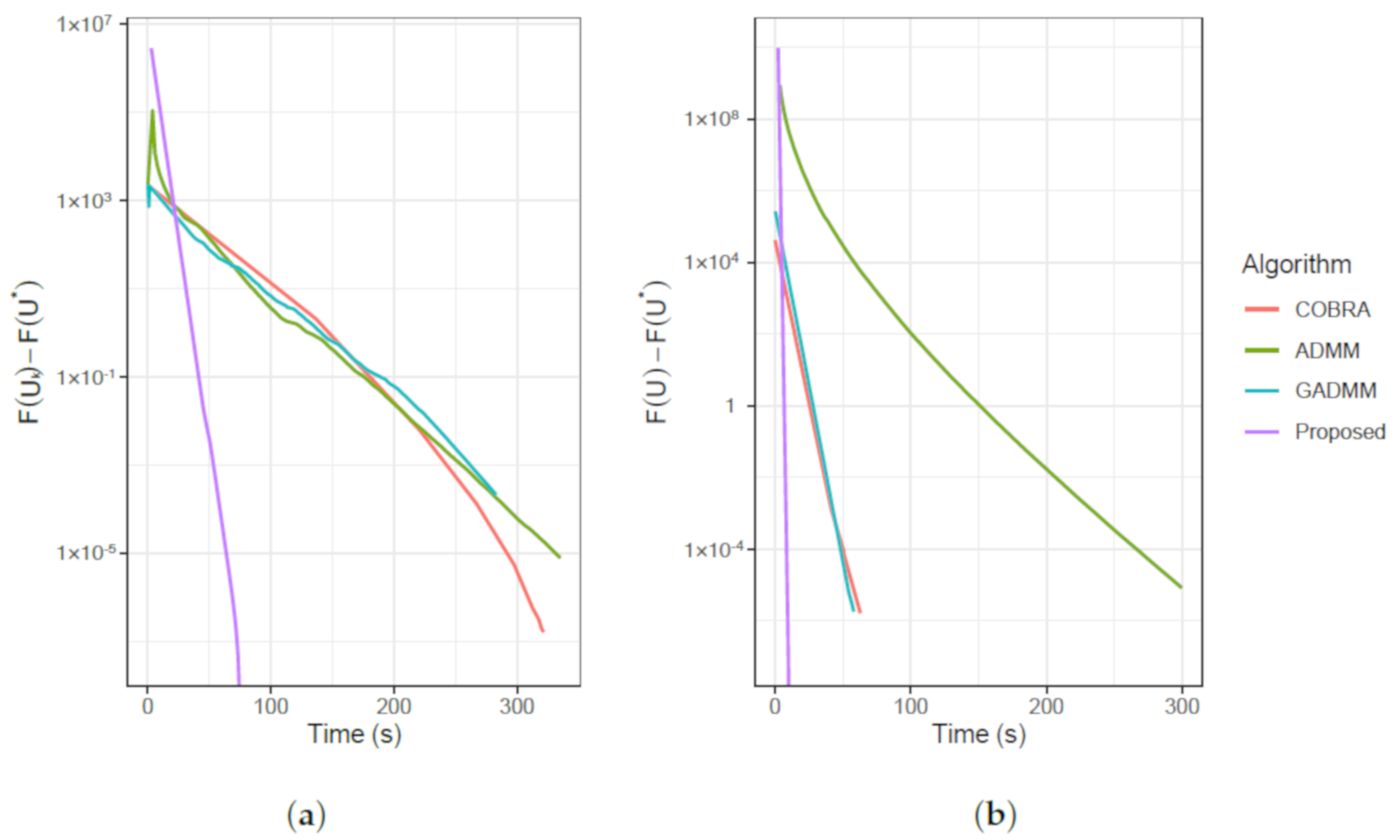
- Objective function error:
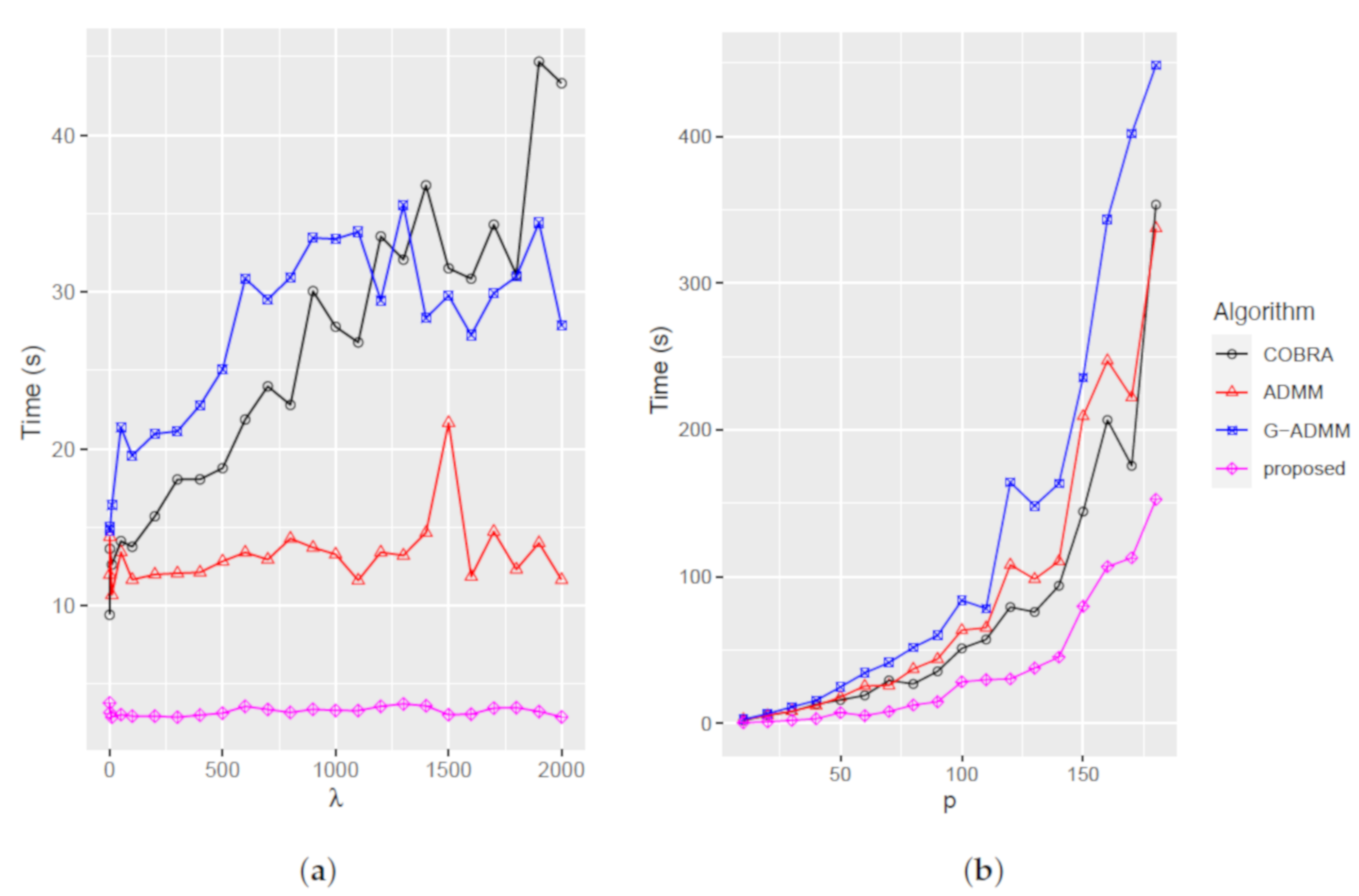
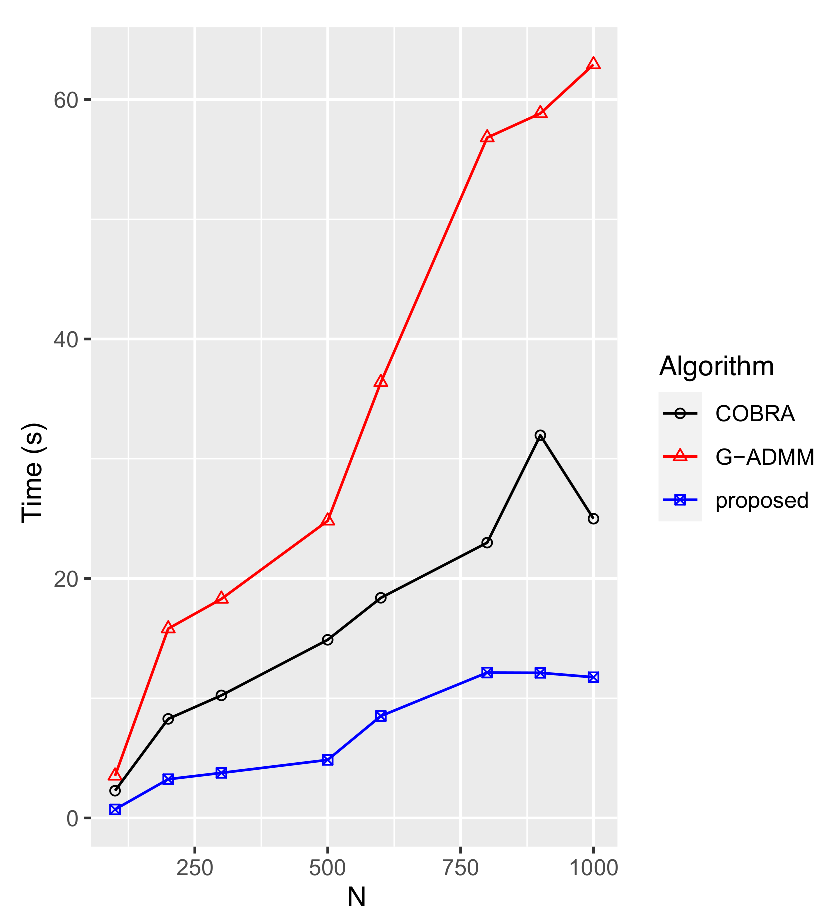
4.1.1. Comparisons
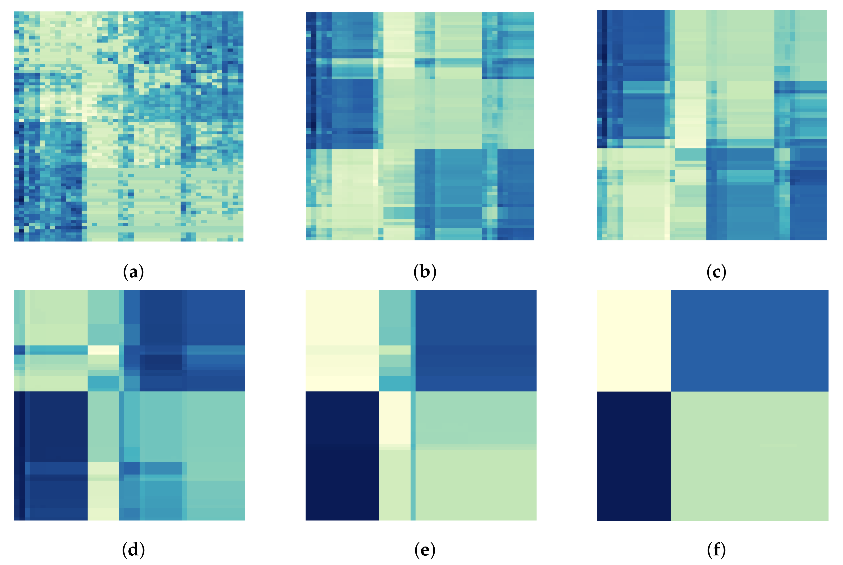
4.1.2. Assessment
4.2. Real Data Analysis
5. Discussion
Author Contributions
Funding
Institutional Review Board Statement
Informed Consent Statement
Data Availability Statement
Acknowledgments
Conflicts of Interest
Abbreviations
| ADMM | alternating direction method of multipliers |
| ALM | augmented Lagrangian method |
| COBRA | convex biclustering algorithm |
| DLBCL | diffuse large-B-cell lymphoma |
| FISTA | fast iterative shrinkage-thresholding algorithm |
| ISTA | iterative shrinkage-thresholding algorithm |
| NAGM | Nesterov’s accelerated gradient method |
| RI | Rand index |
| TCGA | The Cancer Genome Atlas |
Appendix A
Appendix A.1. Proof of Proposition 1
References
- Hartigan, J.A.; Wong, M.A. Algorithm AS 136: A k-means clustering algorithm. J. R. Stat. Soc. Ser. (Appl. Stat.) 1979, 28, 100–108. [Google Scholar] [CrossRef]
- Johnson, S.C. Hierarchical clustering schemes. Psychometrika 1967, 32, 241–254. [Google Scholar] [CrossRef] [PubMed]
- Hastie, T.; Tibshirani, R.; Friedman, J. The Elements of Statistical Learning: Data Mining, Inference, and Prediction; Springer: Berlin/Heidelberg, Germany, 2017. [Google Scholar]
- Hartigan, J.A. Direct clustering of a data matrix. J. Am. Stat. Assoc. 1972, 67, 123–129. [Google Scholar] [CrossRef]
- Cheng, Y.; Church, G.M. Biclustering of expression data. ISMB Int. Conf. Intell. Syst. Mol. Biol. 2000, 8, 93–103. [Google Scholar]
- Tanay, A.; Sharan, R.; Shamir, R. Discovering statistically significant biclusters in gene expression data. Bioinformatics 2002, 18, S136–S144. [Google Scholar] [CrossRef] [Green Version]
- Prelić, A.; Bleuler, S.; Zimmermann, P.; Wille, A.; Bühlmann, P.; Gruissem, W.; Hennig, L.; Thiele, L.; Zitzler, E. A systematic comparison and evaluation of biclustering methods for gene expression data. Bioinformatics 2006, 22, 1122–1129. [Google Scholar] [CrossRef] [PubMed]
- Madeira, S.C.; Oliveira, A.L. Biclustering algorithms for biological data analysis: A survey. IEEE/ACM Trans. Comput. Biol. Bioinform. 2004, 1, 24–45. [Google Scholar] [CrossRef]
- Chi, E.C.; Allen, G.I.; Baraniuk, R.G. Convex biclustering. Biometrics 2017, 73, 10–19. [Google Scholar] [CrossRef]
- Tibshirani, R.; Saunders, M.; Rosset, S.; Zhu, J.; Knight, K. Sparsity and smoothness via the fused lasso. J. R. Stat. Soc. Ser. (Stat. Methodol.) 2005, 67, 91–108. [Google Scholar] [CrossRef] [Green Version]
- Hocking, T.D.; Joulin, A.; Bach, F.; Vert, J.P. Clusterpath an algorithm for clustering using convex fusion penalties. In Proceedings of the 28th International Conference on Machine Learning, ICML 2011, Bellevue, DC, USA, 28 June–2 July 2011; p. 1. [Google Scholar]
- Lindsten, F.; Ohlsson, H.; Ljung, L. Clustering using sum-of-norms regularization: With application to particle filter output computation. In Proceedings of the 2011 IEEE Statistical Signal Processing Workshop (SSP), Nice, France, 28–30 June 2011; pp. 201–204. [Google Scholar]
- Pelckmans, K.; De Brabanter, J.; Suykens, J.A.; De Moor, B. Convex clustering shrinkage. In Proceedings of the PASCALWorkshop on Statistics and Optimization of Clustering Workshop, London, UK, 4–5 July 2005. [Google Scholar]
- Langfelder, P.; Horvath, S. WGCNA: An R package for weighted correlation network analysis. BMC Bioinform. 2008, 9, 1–13. [Google Scholar] [CrossRef] [Green Version]
- Tan, K.M.; Witten, D.M. Sparse biclustering of transposable data. J. Comput. Graph. Stat. 2014, 23, 985–1008. [Google Scholar] [CrossRef] [PubMed] [Green Version]
- Shor, N.Z. Minimization Methods for Non-Differentiable Functions; Springer Science & Business Media: Berlin/Heidelberg, Germany, 2012; Volume 3. [Google Scholar]
- Boyd, S.; Xiao, L.; Mutapcic, A. Subgradient methods. Lect. Notes EE392o Stanf. Univ. Autumn Quart. 2003, 2004, 2004–2005. [Google Scholar]
- Bauschke, H.H.; Combettes, P.L. A Dykstra-like algorithm for two monotone operators. Pac. J. Optim. 2008, 4, 383–391. [Google Scholar]
- Weylandt, M. Splitting methods for convex bi-clustering and co-clustering. In Proceedings of the 2019 IEEE Data Science Workshop (DSW), Minneapolis, MN, USA, 2–5 June 2019; pp. 237–242. [Google Scholar]
- Glowinski, R.; Marroco, A. Sur l’approximation, par éléments finis d’ordre un, et la résolution, par pénalisation-dualité d’une classe de problèmes de Dirichlet non linéaires. ESAIM Math. Model. Numer. Anal.-ModéLisation MathéMatique Anal. NuméRique 1975, 9, 41–76. [Google Scholar] [CrossRef]
- Gabay, D.; Mercier, B. A dual algorithm for the solution of nonlinear variational problems via finite element approximation. Comput. Math. Appl. 1976, 2, 17–40. [Google Scholar] [CrossRef] [Green Version]
- Deng, W.; Yin, W. On the global and linear convergence of the generalized alternating direction method of multipliers. J. Sci. Comput. 2016, 66, 889–916. [Google Scholar] [CrossRef] [Green Version]
- Chi, E.C.; Lange, K. Splitting methods for convex clustering. J. Comput. Graph. Stat. 2015, 24, 994–1013. [Google Scholar] [CrossRef] [PubMed] [Green Version]
- Suzuki, J. Sparse Estimation with Math and R: 100 Exercises for Building Logic; Springer: Berlin/Heidelberg, Germany, 2021. [Google Scholar]
- Bartels, R.H.; Stewart, G.W. Solution of the matrix equation AX+ XB= C [F4]. Commun. ACM 1972, 15, 820–826. [Google Scholar] [CrossRef]
- Goldstein, T.; O’Donoghue, B.; Setzer, S.; Baraniuk, R. Fast alternating direction optimization methods. Siam J. Imaging Sci. 2014, 7, 1588–1623. [Google Scholar] [CrossRef] [Green Version]
- Boyd, S.; Parikh, N.; Chu, E. Distributed Optimization and Statistical Learning via the Alternating Direction Method of Multipliers; Now Publishers Inc.: Boston, MA, USA, 2011. [Google Scholar]
- Abualigah, L.; Diabat, A.; Mirjalili, S.; Abd Elaziz, M.; Gandomi, A.H. The arithmetic optimization algorithm. Comput. Methods Appl. Mech. Eng. 2021, 376, 113609. [Google Scholar] [CrossRef]
- Shimmura, R.; Suzuki, J. Converting ADMM to a Proximal Gradient for Convex Optimization Problems. arXiv 2021, arXiv:2104.10911. [Google Scholar]
- Beck, A.; Teboulle, M. A fast iterative shrinkage-thresholding algorithm for linear inverse problems. Siam J. Imaging Sci. 2009, 2, 183–202. [Google Scholar] [CrossRef] [Green Version]
- Moreau, J.J. Proximité et dualité dans un espace hilbertien. Bull. Soc. Math. France 1965, 93, 273–299. [Google Scholar] [CrossRef]
- Hestenes, M.R. Multiplier and gradient methods. J. Optim. Theory Appl. 1969, 4, 303–320. [Google Scholar] [CrossRef]
- Rockafellar, R.T. The multiplier method of Hestenes and Powell applied to convex programming. J. Optim. Theory Appl. 1973, 12, 555–562. [Google Scholar] [CrossRef]
- Nocedal, J.; Wright, S. Numerical Optimization; Springer Science & Business Media: Berlin/Heidelberg, Germany, 2006. [Google Scholar]
- Nesterov, Y.E. A method for solving the convex programming problem with convergence rate O (1/k2). Dokl. Akad. Nauk Sssr 1983, 269, 543–547. [Google Scholar]
- Boyd, S.; Boyd, S.P.; Vandenberghe, L. Convex Optimization; Cambridge University Press: Cambridge, UK, 2004. [Google Scholar]
- Beck, A. First-Order Methods in Optimization; SIAM: Philadelphia, PA, USA, 2017. [Google Scholar]
- Nemirovski, A.; Yudin, D. Problem Complexity and Method Efficiency in Optimization; John Wiley: Hoboken, NJ, USA, 1983. [Google Scholar]
- Combettes, P.L.; Wajs, V.R. Signal recovery by proximal forward-backward splitting. Multiscale Model. Simul. 2005, 4, 1168–1200. [Google Scholar] [CrossRef] [Green Version]
- Rand, W.M. Objective criteria for the evaluation of clustering methods. J. Am. Stat. Assoc. 1971, 66, 846–850. [Google Scholar] [CrossRef]
- Weylandt, M.; Nagorski, J.; Allen, G.I. Dynamic visualization and fast computation for convex clustering via algorithmic regularization. J. Comput. Graph. Stat. 2020, 29, 87–96. [Google Scholar] [CrossRef] [Green Version]
- Koboldt, D.; Fulton, R.; McLellan, M.; Schmidt, H.; Kalicki-Veizer, J.; McMichael, J.; Fulton, L.; Dooling, D.; Ding, L.; Mardis, E.; et al. Comprehensive molecular portraits of human breast tumours. Nature 2012, 490, 61–70. [Google Scholar]
- Rosenwald, A.; Wright, G.; Chan, W.C.; Connors, J.M.; Campo, E.; Fisher, R.I.; Gascoyne, R.D.; Muller-Hermelink, H.K.; Smeland, E.B.; Giltnane, J.M.; et al. The use of molecular profiling to predict survival after chemotherapy for diffuse large-B-cell lymphoma. N. Engl. J. Med. 2002, 346, 1937–1947. [Google Scholar] [CrossRef] [PubMed]
- Lee, M.; Shen, H.; Huang, J.Z.; Marron, J. Biclustering via sparse singular value decomposition. Biometrics 2010, 66, 1087–1095. [Google Scholar] [CrossRef] [PubMed]
- Wang, M.; Allen, G.I. Integrative generalized convex clustering optimization and feature selection for mixed multi-view data. J. Mach. Learn. Res. 2021, 22, 1–73. [Google Scholar]


| Differentiable | Non-Differentiable | |
|---|---|---|
| Ordinary | Gradient descent | Proximal gradient descent (e.g., ISTA [30]) |
| Accelated | NAGM [35] | FISTA [30] |
| Setting | Algorithm | Rand Index | |||
|---|---|---|---|---|---|
| Setting 1 | COBRA | 0.874 | 0.875 | 0.999 | 0.931 |
| ADMM | 0.872 | 0.875 | 0.999 | 0.931 | |
| G-ADMM | 0.874 | 0.875 | 0.874 | 0.872 | |
| Proposed | 0.875 | 0.875 | 0.999 | 0.931 | |
| Setting 2 | COBRA | 0.928 | 0.932 | 0.994 | 0.999 |
| ADMM | 0.928 | 0.935 | 0.994 | 0.999 | |
| G-ADMM | 0.928 | 0.934 | 0.981 | 0.936 | |
| Proposed | 0.928 | 0.934 | 0.994 | 0.999 | |
| Setting 3 | COBRA | 0.959 | 0.962 | 0.962 | 0.999 |
| ADMM | 0.961 | 0.962 | 0.962 | 0.998 | |
| G-ADMM | 0.959 | 0.962 | 0.967 | 0.967 | |
| Proposed | 0.961 | 0.962 | 0.962 | 0.999 | |
| Setting 4 | COBRA | 0.870 | 0.870 | 0.870 | 0.935 |
| ADMM | 0.870 | 0.868 | 0.871 | 0.933 | |
| G-ADMM | 0.870 | 0.870 | 0.871 | 0.871 | |
| Proposed | 0.870 | 0.870 | 0.871 | 0.935 | |
| Setting 5 | COBRA | 0.934 | 0.934 | 0.934 | 0.964 |
| ADMM | 0.934 | 0.932 | 0.934 | 0.964 | |
| G-ADMM | 0.934 | 0.934 | 0.932 | 0.932 | |
| Proposed | 0.934 | 0.934 | 0.934 | 0.964 | |
| Setting 6 | COBRA | 0.960 | 0.960 | 0.962 | 0.962 |
| ADMM | 0.961 | 0.962 | 0.962 | 0.962 | |
| G-ADMM | 0.960 | 0.962 | 0.962 | 0.960 | |
| Proposed | 0.961 | 0.962 | 0.962 | 0.962 | |
Publisher’s Note: MDPI stays neutral with regard to jurisdictional claims in published maps and institutional affiliations. |
© 2021 by the authors. Licensee MDPI, Basel, Switzerland. This article is an open access article distributed under the terms and conditions of the Creative Commons Attribution (CC BY) license (https://creativecommons.org/licenses/by/4.0/).
Share and Cite
Chen, J.; Suzuki, J. An Efficient Algorithm for Convex Biclustering. Mathematics 2021, 9, 3021. https://doi.org/10.3390/math9233021
Chen J, Suzuki J. An Efficient Algorithm for Convex Biclustering. Mathematics. 2021; 9(23):3021. https://doi.org/10.3390/math9233021
Chicago/Turabian StyleChen, Jie, and Joe Suzuki. 2021. "An Efficient Algorithm for Convex Biclustering" Mathematics 9, no. 23: 3021. https://doi.org/10.3390/math9233021
APA StyleChen, J., & Suzuki, J. (2021). An Efficient Algorithm for Convex Biclustering. Mathematics, 9(23), 3021. https://doi.org/10.3390/math9233021