Optimal Control Applied to Vaccination and Testing Policies for COVID-19

Abstract

In this paper, several policies for controlling the spread of SARS-CoV-2 are determined under the assumption that a limited number of effective COVID-19 vaccines and tests are available. These policies are calculated for different vaccination scenarios representing vaccine supply and administration restrictions, plus their impacts on the disease transmission are analyzed. The policies are determined by solving optimal control problems of a compartmental epidemic model, in which the control variables are the vaccination rate and the testing rate for the detection of asymptomatic infected people. A combination of the proportion of threatened and deceased people together with the cost of vaccination of susceptible people, and detection of asymptomatic infected people, is taken as the objective functional to be minimized, whereas different types of algebraic constraints are considered to represent several vaccination scenarios. A direct transcription method is employed to solve these optimal control problems. More specifically, the Hermite–Simpson collocation technique is used. The results of the numerical experiments show that the optimal control approach offers healthcare system managers a helpful resource for designing vaccination programs and testing plans to prevent COVID-19 transmission.

1. Introduction

In this paper, the problem of finding the best policies for controlling the transmission of the COVID-19 is formulated as an optimal control problem (OCP). In particular, the optimal vaccination rate and the optimal testing rate for the detection of asymptomatic infected people must be determined. Several scenarios are considered, each of which is represented by a distinct algebraic constraint in the OCP, in which the number of vaccine accessible every day is limited or the overall number of vaccine supplies along the time period considered is restricted. In the formulation of the OCP, a compartmental epidemic model is used to model the SARS-CoV-2 transmission dynamics and its interaction with the control policies. A combination of the proportion of threatened and deceased people with the cost of vaccination of susceptible people and detection of asymptomatic infected people is employed as the objective functional in the OCP.

Various compartmental models have been formulated, which analyze different aspects of the COVID-19 disease. In [1], a taxonomy of models is considered, and their contributions to the analysis of the disease are explored. In [2], the spread of the disease is studied, in which the number of susceptible individuals does not decrease monotonically and the total population is not kept constant per se. The transmissibility of super-spreaders individuals is analyzed in [3]. A climate-dependent epidemic model is developed in [4] in order to determine whether climate can affect transmission of SARS-CoV-2. In [5], several simulations are presented that used a population pharmacokinetic model to predict plasma concentration-time profiles after single or repeated fasted administrations of ivermectin. In [6], containment measures are modeled by considering a time-dependent modulation of bare infectivity and simulating the combined effect of asymptomatic onset, testing policies, and quarantine. In [7], an extended susceptible–exposed–infected–recovered (SEIR) model is proposed that accounts for social and non-pharmaceutical prevention interventions in order to estimate the size of an epidemic and forecast the extent of public health risks associated with epidemics. In [8,9], a modified SEIR model is proposed which predicts the effect of the strategies used to flatten the power-law curves. A model with eight stages of infection is presented in [10], in which several strategies are considered, including social distancing, testing, and contact tracing. In [11], the effects of major interventions are studied using a model that calculates backwards from observed deaths to estimate transmission that occurred weeks before. In [12], several regional-scale models are presented with the aim of measuring and forecasting the impacts of social distancing in the absence of a vaccine or antiviral therapies. The individual’s behavior in spreading and controlling the epidemic is analyzed in [13] using a model that includes a vaccinated term in order to predict how vaccination could control the epidemic. In [14], a generalized SEIR model is considered, in which vaccination and quarantining strategies are modeled as controllers that are derived using the Lyapunov theory.

The optimal control approach has been extensively employed for compartmental epidemic models. For the sake of brevity, the research we mention in the following is limited, and these studies deal with different issues related to the COVID-19 pandemic. The impacts of non-pharmaceutical interventions on the dynamics of COVID-19 transmission are analyzed in [15] by means of a case study. Non-pharmaceutical measures such as isolation, quarantine, and public health education are studied as time-dependent interventions in [16] to identify their contributions to the COVID-19 transmission dynamics. An OCP with free terminal time of the SARS-CoV-2 transmission dynamics is defined in [17], with the goal of reducing the sizes of susceptible, infected, exposed, and asymptomatic proportions to eradicate the infection via quarantine and treatment of infected people. A susceptible–infected–recovered (SIR) model of the COVID-19 pandemic is considered in [18], in which the transmission rate of the disease and the efficiency of treatments are subject to uncertainty. The impacts of delays in applying preventive precautions against the spread of the COVID-19 pandemic are assessed in [19] through a mathematical model with multiple delays. The dynamics of an SIR model of SARS-CoV-2 transmission with interacting populations is approximated in [20], in which the optimal vaccine allocation problem is reduced to a knapsack problem. An OCP for a fractional system of the COVID-19 transmission dynamics is designed in [21], in which several non-pharmaceutical intervention policies are incorporated. An OCP of a SEIR model of the COVID-19 outbreak in Ireland is formulated in [22], in which the costs of various non-pharmaceutical interventions are minimized, subject to hospital admissions never exceeding a threshold value corresponding to health service capacity. An OCP with mixed constraints is formulated in [23] to describe vaccination schedules, in which the solution minimizes the burden of COVID-19 quantified by the number of disability-adjusted years of life lost. The optimal vaccine allocation for four optimality criteria, namely, deaths, symptomatic infections, and maximum intensive care units (ICU) and non-ICU hospitalizations is determined under several scenarios in [24] using an age-stratified mathematical model. The impact of COVID-19 vaccine optimization and prioritization policies based on cumulative incidence, mortality, and years of life lost is quantified in [25]. In [26], the OCP of a susceptible–exposed–infected–quarentined–recovered (SEIQR) model is considered, which incorporates three types of control strategies, namely, the use of face-masks, hand sanitizer, and social distancing; the treatment of COVID-19 patients and active screening with testing; and prevention against recurrence and reinfection of humans who have recovered from COVID-19. The OCP of an epidemic model that simultaneously considers multiple viral strains and reinfection due to waning immunity is formulated in [27], which seeks a trade-off between the societal and economic costs of mitigation.

This paper addresses the problem of finding and comparing the best vaccination and testing policies for an epidemic model of COVID-19 transmission developed from the compartmental model presented in [10]. These policies are determined by stating OCPs with different types of algebraic constraints that are solved using a direct transcription technique, which allows inequality and equality constraints to be easily incorporated. More specifically, the Hermite–Simpson collocation method [28] is employed, which turns the OCP into a nonlinear programming (NLP) problem, which is solved using the NLP solver IPOPT [29]. The results of the numerical experiments show that this optimal control approach offers healthcare system managers a helpful resource for designing vaccination programs and testing plans to prevent COVID-19 transmission.

The paper is organized as follows: The mathematical model of the SARS-CoV-2 virus transmission dynamics with vaccination and testing policies is presented in Section 2.1. Various vaccination scenarios described by different kinds of constraints are introduced in Section 2.2, along with the formulation of the corresponding OCP of the COVID-19 epidemic model. The technique used to solve the OCP numerically is described in Section 2.3. The results of several numerical experiments are reported and analyzed in Section 3. Finally, some conclusions are drawn in Section 5.

2. Materials and Methods

2.1. Mathematical Model

The mathematical model with vaccination and testing policies considered in this paper was derived from the compartmental epidemic model proposed in [10], which allows the possibility of including social distancing policies and testing campaigns to detect infected people. This model, denoted as SIDARTHE, consists of 8 compartments: susceptible (S), infected (I), diagnosed (D), ailing (A), recognized (R), threatened (T), healed (H), and extinct (E) people. In addition, the model used in this paper contains an immunity loss term and a vaccination term as shown in Figure 1.

The state-space representation of the SIDARTHE model is given by the following set of ordinary differential equations (ODEs):

$$\begin{array}{ccc}\hfill \dot{S}\left(t\right)& = & -S\left(t\right)\left(\alpha I\left(t\right)+\beta D\left(t\right)+\gamma A\left(t\right)+\delta R\left(t\right)\right)+\iota H\left(t\right)-\varphi v\left(t\right)S\left(t\right),\hfill \end{array}$$

(1)

$$\begin{array}{ccc}\hfill \dot{I}\left(t\right)& = & S\left(t\right)\left(\alpha I\left(t\right)+\beta D\left(t\right)+\gamma A\left(t\right)+\delta R\left(t\right)\right)-(\epsilon \left(t\right)+\zeta +\lambda )I\left(t\right),\hfill \end{array}$$

(2)

$$\begin{array}{ccc}\hfill \dot{D}\left(t\right)& = & \epsilon \left(t\right)I\left(t\right)-(\eta +\rho )D\left(t\right),\hfill \end{array}$$

(3)

$$\begin{array}{ccc}\hfill \dot{A}\left(t\right)& = & \zeta I\left(t\right)-(\theta +\mu +\kappa )A\left(t\right),\hfill \end{array}$$

(4)

$$\begin{array}{ccc}\hfill \dot{R}\left(t\right)& = & \eta D\left(t\right)+\theta A\left(t\right)-(\nu +\xi )R\left(t\right),\hfill \end{array}$$

(5)

$$\begin{array}{ccc}\hfill \dot{T}\left(t\right)& = & \mu A\left(t\right)+\nu R\left(t\right)-(\sigma +\tau )T\left(t\right),\hfill \end{array}$$

(6)

$$\begin{array}{ccc}\hfill \dot{H}\left(t\right)& = & \lambda I\left(t\right)+\rho D\left(t\right)+\kappa A\left(t\right)+\xi R\left(t\right)+\sigma T\left(t\right)-\iota H\left(t\right)+\varphi v\left(t\right)S\left(t\right),\hfill \end{array}$$

(7)

$$\begin{array}{ccc}\hfill \dot{E}\left(t\right)& = & \tau T\left(t\right).\hfill \end{array}$$

(8)

The ODE system (1)–(8) consists of 8 state variables, 2 control inputs, and 17 parameters. The variables with time derivatives are the state variables of the system. In particular, $S\left(t\right)$ represents the proportion of people susceptible to infection, $I\left(t\right)$ represents the proportion of asymptomatic or paucisymptomatic infected people that remain undetected, $D\left(t\right)$ represents the proportion of asymptomatic infected people that are detected, $A\left(t\right)$ represents the proportion of symptomatic infected people that remain undetected, $R\left(t\right)$ represents the proportion of symptomatic infected people that are detected, $T\left(t\right)$ represents the proportion of infected people with life-threatening symptoms that are detected, $H\left(t\right)$ represents the proportion of people which are infected but recover or susceptible people who become immune through vaccination, and $E\left(t\right)$ represents the proportion of deceased people.

As shown in [10], the SIDARTHE model is a compartmental system, which demonstrates the mass conservation property, namely,

$$\begin{array}{c}\hfill \dot{S}\left(t\right)+\dot{I}\left(t\right)+\dot{D}\left(t\right)+\dot{A}\left(t\right)+\dot{R}\left(t\right)+\dot{T}\left(t\right)+\dot{H}\left(t\right)+\dot{E}\left(t\right) = 0.\end{array}$$

Hence, the sum of the compartments, which represents the total population, is constant. More specifically, since the variables denote population fractions, it is assumed that

$$\begin{array}{c}\hfill S\left(t\right)+I\left(t\right)+D\left(t\right)+A\left(t\right)+R\left(t\right)+T\left(t\right)+H\left(t\right)+E\left(t\right) = 1,\end{array}$$

where 1 represents the total population. Therefore, in the formulation of the infection force the total population is assumed to be 1, and $\alpha$, $\beta$, $\gamma$, and $\delta$, respectively, denote the probability of disease transmission in a single contact multiplied by the average number of contacts per person due to contacts between a susceptible subject and an infected, a diagnosed, an ailing, and a recognized subject, respectively. Moreover the possibility of presymptomatic transmission of the disease is assumed. For this reason, a compartment of exposed people is not included in the formulation of the model.

The control variables of the ODE system (1)–(8) are $v\left(t\right)$ and $\epsilon \left(t\right)$. The control variable $v\left(t\right)$ denotes the vaccination rate, which ranges from 0 to $v_{\mathbf{u}}$, where $v_{\mathbf{u}}$ is an upper bound that must be provided by the designers of the optimal control model. Therefore, the vaccination policy in model (1)–(8) is represented by the term $\varphi v\left(t\right)S\left(t\right)$, where parameter $\varphi$ represents the vaccine efficacy level. Thus, in this model, only the susceptible people are assumed to be vaccinated. The control variable $\epsilon \left(t\right)$ denotes the testing rate for the detection of asymptomatic infected people, which ranges from ${\epsilon }_L$ to ${\epsilon }_{\mathbf{u}}$, where ${\epsilon }_L$ and ${\epsilon }_{\mathbf{u}}$ represent a lower and an upper bound, respectively, which must be provided by the designers of the optimal control model. Notice that, in [10], $\epsilon$ is considered as a constant parameter of the SIDARTHE model.

The other symbols of the ODE system (1)–(8) are parameters. The parameters $\alpha ,\beta ,\gamma$, and $\delta$ represent the transmission rate due to contacts between a susceptible person and an infected, a diagnosed, an ailing, and a recognized person, respectively. The parameter $\theta$ represents the testing rate for the detection of symptomatic infected people. The parameters $\zeta$ and $\eta$ represent the rate at which an infected person, unaware and aware of being infected, respectively, develops clinically relevant symptoms. The parameters $\mu$ and $\nu$ represent the rates at which undetected and detected infected people, respectively, develop life-threatening symptoms. The parameter $\tau$ represents the mortality rate for infected people with life-threatening symptoms. The parameters $\lambda ,\kappa ,\xi ,\rho$, and $\sigma$ represent the recovery rates for the infected, diagnosed, ailing, recognized, and threatened people, respectively.

As shown in [10], the parameters $\alpha ,\beta ,\gamma$, and $\delta$ can be modified according to social distancing actions, such as closing schools, remote working, and lockdown. Moreover, $\theta$ reflects the number of tests performed on the symptomatic infected people and can be increased by enforcing a massive testing campaign. The parameters $\zeta ,\eta ,\mu ,\nu ,\tau ,\lambda ,\kappa ,\xi ,\rho$, and $\sigma$ are disease-dependent. The parameters $\zeta$, $\eta$, $\mu$, $\nu$, and $\tau$ may be reduced by means of improved therapies, whereas $\lambda ,\kappa ,\xi ,\rho$, and $\sigma$ can be increased through improved treatments. Notice that, in model (1)–(8), the risk of contagion due to a contact between a susceptible person and a threatened person, and the probability rate of becoming susceptible again, after having recovered from the infection, are assumed negligible.

As mentioned above, in this paper, an immunity loss term and an immunization term are added to the model proposed in [10] and various OCPs are formulated for different vaccination scenarios modeled using different types of algebraic constraints, in which the vaccination rate $v\left(t\right)$ and the testing rate for the detection of asymptomatic infected people $\epsilon \left(t\right)$ are the control variables. The immunity loss is represented by the term $\iota H\left(t\right)$, which allows the proportion of people susceptible to reinfection to be modeled, where parameter $\iota$ represents the immunity loss rate of recovered people. The duration of immunity against COVID-19 is still an open research question. In the last year, several works have proposed different epidemic models, including a wide variety of immunity loss rates, which assume a duration of the immunity ranging from a few months to several years [30,31,32,33,34,35]. In this work, the sensitivity of the OCP to the immunity loss rate is analyzed, in which the duration of the immunity is assumed to be between 6 months and 3 years [36,37].

2.2. Vaccination Scenarios

Vaccination and testing policies to control the spread of COVID-19 are obtained in this paper solving OCPs in which the dynamical system is described by model (1)–(8). Different vaccination scenarios are studied, which are represented by constraints of the OCP. Depending on the vaccination scenario and the objective functional of the OCP, it is possible to obtain distinct vaccination and testing policies. In particular, the following three scenarios are considered in this paper:

• Scenario 1: During the time period under consideration, the total number of administered vaccines is assumed to be fixed. Thus, in this scenario, all vaccine supplies must be used.
• Scenario 2: During the time period under consideration, the total number of administered vaccines is limited. Thus, in this scenario, the use of all vaccine supplies is not mandatory.
• Scenario 3: The number of vaccines administered daily is limited.

Notice that the first scenario can be represented by an isoperimetric constraint, the second scenario corresponds to a state constraint, and a mixed state-control constraint can be used to model the third scenario.

A combination of the proportion of threatened and deceased people, together with the cost of vaccination of susceptible people and detection of asymptomatic infected people, is considered as the objective functional to be minimized in all the three scenarios, namely,

$$\begin{array}{c}\hfill J(T\left(t\right),E\left(t\right),v\left(t\right),\epsilon \left(t\right)) = {\int }_{t_I}^{t_F}\left(C_1\left(T\left(t\right)+E\left(t\right)\right)+C_2{v}^2\left(t\right)+C_3{\epsilon }^2\left(t\right)\right)dt,\end{array}$$

(9)

where $C_i\in [0,1],i = 1,2,3$, are weighting parameters. They are non-dimensional quantities that range between 0 and 1, which must be provided by the designers of the optimal control model according to their preferences. For example, larger values of $C_2$ give more importance to the vaccination cost, whereas larger values of $C_3$ give more importance to the cost associated with testing for the detection of asymptomatic infected people.

2.2.1. Scenario 1

It is assumed in this case that the number of vaccines available during the time period under consideration is known and that they are all administered. Therefore, the number of vaccines administered during the time period $[t_I,t_F]$ is fixed. Following [38], this scenario can be represented by the isoperimetric constraint

$$\begin{array}{c}\hfill {\int }_{t_I}^{t_F}v\left(t\right)S\left(t\right) = V_T,\end{array}$$

(10)

where $V_T$ denotes the total number of susceptible people that are vaccinated over the time period $[t_I,t_F]$. The integral constraint (10) can be handled by creating a new state variable $W\left(t\right)$ and a new differential equation with its associated boundary conditions, as shown below:

$$\begin{array}{ccc}\hfill \dot{W}\left(t\right)& = & v\left(t\right)S\left(t\right),\hfill \\ \hfill W\left(t_I\right)& = & 0,\hfill \\ \hfill W\left(t_F\right)& = & V_T.\hfill \end{array}$$

2.2.2. Scenario 2

Unlike scenario 1, where it is assumed that the number of vaccines available during the time period under consideration is known and they are all administered, in this case it is assumed that they can all be administered or not. Following [39], this condition can be represented by the inequality constraint

$$\begin{array}{c}\hfill W\left(t_F\right)\le V_T.\end{array}$$

(11)

Notice that the inequality constraint (11) is a state constraint, which represents an overall upper limit on vaccine supplies over the given time period. Moreover, if inequality constraint (11) is saturated in the solution of the corresponding OCP, then scenarios 1 and 2 will provide the same vaccination policy.

2.2.3. Scenario 3

It is assumed in this case that the number of vaccines available each day is known and that they can all be administered or none at all.Following [39], this scenario can be represented by the inequality constraint

$$\begin{array}{c}\hfill v\left(t\right)S\left(t\right)\le V_0,\mathrm{with}t\in [t_I,t_F].\end{array}$$

(12)

Notice that the inequality constraint (12) is a mixed state-control constraint, in which the parameter $V_0$ denotes an upper bound on the number of susceptible people vaccinated daily.

Therefore, the optimal control of the SIDARTHE model (1)–(8) with mixed state-control constraint is formulated as follows:

$$\begin{array}{ccc}& & \underset{v\left(t\right),\epsilon \left(t\right)}{min}J(T\left(t\right),E\left(t\right),v\left(t\right),\epsilon \left(t\right)),\hfill \\ & & \mathrm{subject}\mathrm{to}:\hfill \end{array}$$

(13)

$$\begin{array}{ccc}& & \dot{S}\left(t\right) = -S\left(t\right)\left(\alpha I\left(t\right)+\beta D\left(t\right)+\gamma A\left(t\right)+\delta R\left(t\right)\right)+\iota H\left(t\right)-\varphi v\left(t\right)S\left(t\right),\hfill \end{array}$$

(14)

$$\begin{array}{ccc}& & \dot{I}\left(t\right) = S\left(t\right)\left(\alpha I\left(t\right)+\beta D\left(t\right)+\gamma A\left(t\right)+\delta R\left(t\right)\right)-(\epsilon \left(t\right)+\zeta +\lambda )I\left(t\right),\hfill \end{array}$$

(15)

$$\begin{array}{ccc}& & \dot{D}\left(t\right) = \epsilon \left(t\right)I\left(t\right)-(\eta +\rho )D\left(t\right),\hfill \end{array}$$

(16)

$$\begin{array}{ccc}& & \dot{A}\left(t\right) = \zeta I\left(t\right)-(\theta +\mu +\kappa )A\left(t\right),\hfill \end{array}$$

(17)

$$\begin{array}{ccc}\hfill & & \dot{R}\left(t\right) = \eta D\left(t\right)+\theta A\left(t\right)-(\nu +\xi )R\left(t\right),\hfill \end{array}$$

(18)

$$\begin{array}{ccc}\hfill & & \dot{T}\left(t\right) = \mu A\left(t\right)+\nu R\left(t\right)-(\sigma +\tau )T\left(t\right),\hfill \end{array}$$

(19)

$$\begin{array}{c}\dot{H}\left(t\right) = \lambda I\left(t\right)+\rho D\left(t\right)+\kappa A\left(t\right)+\xi R\left(t\right)+\sigma T\left(t\right)-\iota H\left(t\right)+\varphi v\left(t\right)S\left(t\right),\hfill \end{array}$$

(20)

$$\begin{array}{ccc}\hfill & & \dot{E}\left(t\right) = \tau T\left(t\right),\hfill \end{array}$$

(21)

$$\begin{array}{ccc}\hfill & & \mathbf{u}\left(t\right)S\left(t\right)-V_0\le 0,\hfill \end{array}$$

(22)

$$\begin{array}{ccc}\hfill & & S\left(t_I\right) = S_I,I\left(t_I\right) = I_I,D\left(t_I\right) = D_I,A\left(t_I\right) = A_I,\hfill \end{array}$$

(23)

$$\begin{array}{ccc}\hfill & & R\left(t_I\right) = R_I,T\left(t_I\right) = T_I,H\left(t_I\right) = H_I,E\left(t_I\right) = E_I,\hfill \end{array}$$

(24)

where $J\left(T\right(t),E(t),v(t),\epsilon (t\left)\right)$ is defined as in (9), $v\left(t\right)\in [0,v_{\mathbf{u}}]$, and $\epsilon \left(t\right)\in [{\epsilon }_L,{\epsilon }_{\mathbf{u}}]$. Notice that the OCPs with isoperimetric and state constraints can be stated in a similar way.

2.3. Numerical Resolution of the Optimal Control Problem

The OCP with isoperimetric, state, and mixed state-control constraints presented in Section 2.2 can be all expressed in the following more general form:

$$\begin{array}{ccc}& & \underset{\mathbf{u}\left(t\right)}{min}\mathcal{J}(\mathbf{x}\left(t\right),\mathbf{u}\left(t\right)) = \mathcal{M}\left(\mathbf{x}\left(t_F\right)\right)+{\int }_{t_I}^{t_F}\mathcal{L}(\mathbf{x}\left(t\right),\mathbf{u}\left(t\right))dt,\hfill \\ & & \mathrm{subject}\mathrm{to}:\hfill \end{array}$$

(25)

$$\begin{array}{ccc}& & \dot{\mathbf{x}}\left(t\right) = \mathbf{f}(\mathbf{x}\left(t\right),\mathbf{u}\left(t\right)),\hfill \end{array}$$

(26)

$$\begin{array}{ccc}& & \mathbf{g}(\mathbf{x}\left(t\right),\mathbf{u}\left(t\right)) \le 0,\hfill \end{array}$$

(27)

$$\begin{array}{ccc}& & \mathbf{x}\left(t_I\right) = {\mathbf{x}}_I,\mathbf{x}\left(t_F\right) = {\mathbf{x}}_F.\hfill \end{array}$$

(28)

In (25)–(28), the independent variable t represents the time, with $t_I$ and $t_F$ being the initial and final times, whereas $\mathbf{x}\left(t\right)$ and $\mathbf{u}\left(t\right)$ represent the vectors of state and control variables, respectively. The vectors ${\mathbf{x}}_I$ and ${\mathbf{x}}_F$ represent the initial and final states, respectively. The objective functional $\mathcal{J}(·)$ in (25) is given in Bolza form, which combines a Mayer term $\mathcal{M}(·)$ and a Lagrange term $\mathcal{L}(·)$. The set of differential Equation (26) describes the dynamical system, Equation (27) represents the set of algebraic constraints, and Equation (28) denotes the boundary conditions. Notice that the Lagrange term can be rewritten as a Mayer term by introducing a new state variable, $x_M\left(t\right)$, and adding a new differential equation with its associated initial condition:

$$x_M\left(t\right) = \mathcal{L}\left(\mathbf{x}\right(t),\mathbf{u}\left(t\right)),$$

$$x_M\left(t_I\right) = 0.$$

A direct transcription approach is used to obtain numerical solutions of the OCP (25)–(28), which makes it easy to deal with inequality and equality constraints. Specifically, the Hermite–Simpson collocation method [28] is employed to transcribe the OCP (25)–(28) into a NLP problem, the constraints of which consist of the Hermite–Simpson system constraints that correspond to the differential constraint (26), the algebraic constraints (27), and the boundary conditions (28). The resulting NLP problem is then solved by means of the open-source IPOPT solver [29].

3. Results

To illustrate the application of the proposed approach to the computation of the optimal vaccination and testing policies for the SIDARTHE compartmental model (1)–(8), several numerical experiments have been carried out assuming the testing policy for the detection of asymptomatic infected people and the use of the different vaccination strategies introduced in Section 2.2. It has been assumed that two doses of vaccine are required to develop immunity, and following the Government of Spain’s vaccination plan [40], in which 1 million vaccinations per week have been scheduled using the approximately 13,000 available public health centers, the upper bound on the vaccination rate has been set to $v_{\mathbf{u}} = 0.0035$. Moreover, the following initial conditions have been assumed: $S_0 = 0.8474,$$I_0 = 0.0008,D_0 = 0.0008,A_0 = 0.0002,R_0 = 0.00017,T_0 = 0.00003,H_0 = 0.1489$, and $E_0 = 0.0017$, which reflect the epidemiological situation of COVID-19 described in the ENE-COVID seroprevalence study (data ending December 2020) [41], according to which almost 15% of the Spanish population overcame the disease, and the Government of Spain reports daily [40] regarding the numbers of hospitalizations, UCI admisssions, deaths, and (detected) infected people.

Notice that, in [10], a best-fit approach was adopted to find the values of the parameters of the SIDARTHE model. More specifically, using real data, several sets of parameters were estimated in [10] under the assumptions of different scenarios of implementation of countermeasures adopted by policymakers, which ranged from milder to stronger mitigation measures.

In this work, Spain was considered the focus, and the chosen parameters reflect the countermeasures proposed by the Government of Spain and the situation in Spain at the end of December 2020. Thus, the numerical experiments have been conducted assuming the implementation of mild countermeasures to reduce the transmission of the SARS-CoV-2, such as basic social distancing, hygiene, and behavioral recommendations; screening of symptomatic people; and partial mobility restrictions. More specifically, according to [10], the values of the parameters of the SIDARTHE model used in the numerical experiments are reported in

Table 1. Values of the parameters of the SIDARTHE model used in the numerical experiments.

Parameter	Value	Unit
$\alpha$	$0.330$	people per day
$\beta$	$0.005$	people per day
$\gamma$	$0.110$	people per day
$\delta$	$0.005$	people per day
$\theta$	$0.371$	dimensionless
$\zeta$	$0.025$	days${}^{-1}$
$\eta$	$0.025$	days${}^{-1}$
$\mu$	$0.008$	days${}^{-1}$
$\nu$	$0.015$	days${}^{-1}$
$\tau$	$0.010$	days${}^{-1}$
$\lambda$	$0.080$	days${}^{-1}$
$\kappa$	$0.020$	days${}^{-1}$
$\xi$	$0.020$	days${}^{-1}$
$\rho$	$0.020$	days${}^{-1}$
$\sigma$	$0.010$	days${}^{-1}$
$\iota$	$0.0009,0.0014,0.0028,0.0056$	days${}^{-1}$
$\varphi$	$0.50,0.75,0.95$	dimensionless

.

3.1. Optimal Vaccination and Testing Policies

Three solutions of the OCP for the SIDARTHE compartmental model (1)–(8) have been computed considering the three vaccination scenarios described in Section 2.2, in which the values of the weighting parameters of the objective functional were set to $C_1 = 1,C_2 = 0.1$, and $C_3 = 0.0001$, and the vaccine efficacy level was set to $\varphi = 0.95$. Moreover, the value of the immunity loss rate was set to $\iota = 0.0009$ and the lower and upper bounds of the testing rate for the detection of asymptomatic infected people were set to ${\epsilon }_L = 0$ and ${\epsilon }_{\mathbf{u}} = 0.20$, respectively.

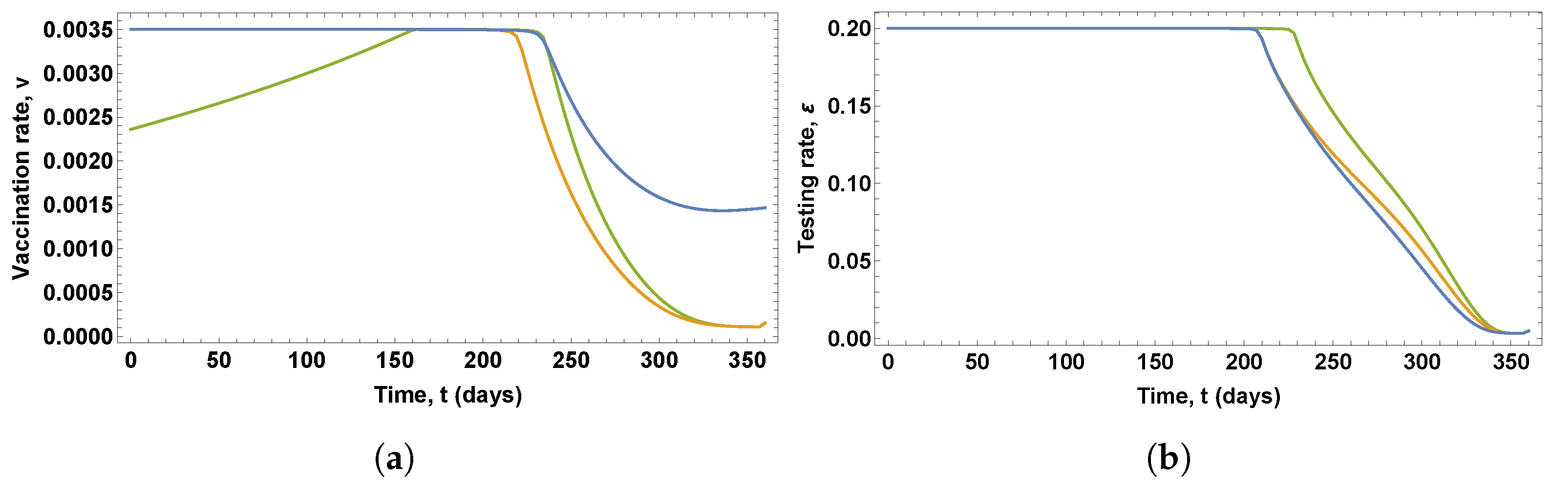
The OCP for scenario 3 was solved in the first place for the sake of comparison, in which, the upper bound of the proportion of susceptible daily vaccinated subjects was set to $V_0 = 0.002$. Then, the upper limit of the OCPs formulated for scenarios 1 and 2 was set to $V_T = 0.6$. Figure 2 shows the control variables obtained in these solutions, which give the optimal vaccination and testing rates, whereas Figure 3 shows the eight state variables corresponding to these optimal control policies.

It can be seen in Figure 2a that the optimal vaccination policies obtained in the solutions of the three OCPs differs considerably. Notice that different optimal vaccination policies were obtained for scenarios 1 and 2, since the state constraint (11) is not saturated in scenario 2, which means that the total number of vaccines is not administered at the end of the time period under consideration. More specifically, $11.17\%$ of the total vaccines are not used. In scenario 1, the optimal vaccination rate is at the maximum value during the first 230 days, then gradually decreases until it reaches $0.0015$, when vaccine stocks are exhausted. In scenario 2, the optimal vaccination rate is at the maximum value during the first 215 days, and then gradually decreases at a higher rate until it reaches zero at the end of the time period under consideration. In scenario 3, the optimal vaccination rate gradually increases during the first 160, takes the maximum value during 80 days, and then decreases at a higher rate until it reaches zero at the end of the time period under consideration.

It can be seen in Figure 2b that the optimal testing policy for the detection of asymptomatic infected people obtained in the solution of the OCP for scenario 3 differs from the optimal testing policy obtained in the solutions of the OCPs for scenarios 1 and 2, which show similar profiles. In the case of scenario 3, the optimal testing rate is at the maximum value during the first 230 days, and then decreases gradually until it reaches zero at the end of the time period under consideration. In the case of scenarios 1 and 2, the optimal testing rate is at the maximum value during the first 210 days, and then decreases gradually, at a slower rate, until it reaches zero at the end of the time period under consideration.

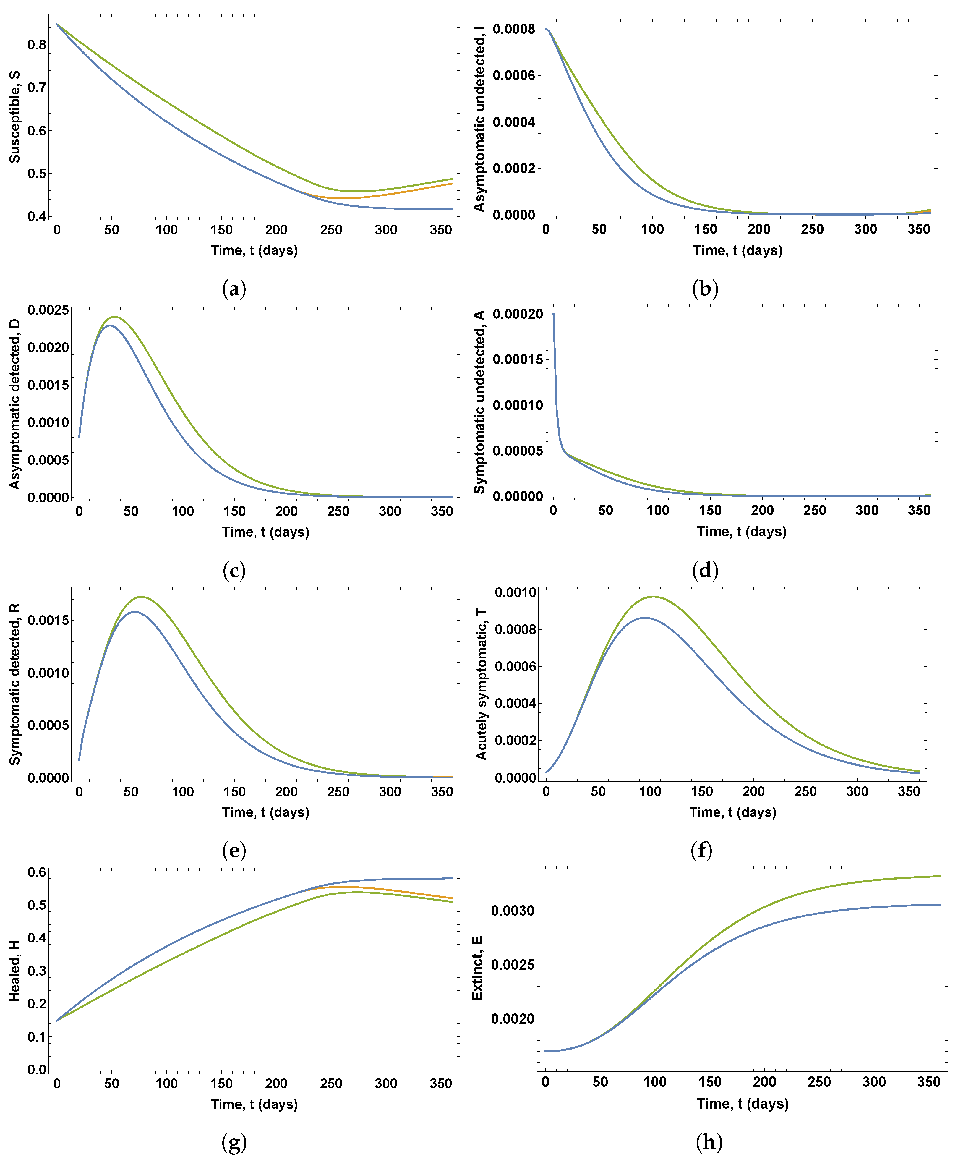
As shown in Figure 3, the different vaccination policies lead to the same behavior for the state variables $I,D,A,R$, and T in the solutions of the OCPs for scenarios 1 and 2, whereas the state variables S and H show a different behavior during the last 120 days. Due to the effect of the immunity loss, one can observe in scenario 2 a new increase in the proportion of people susceptible to infection. Moreover, higher and delayed values for state variables $I,D,A,R$, and T can be observed when the optimal vaccination and testing policies corresponding to scenario 3 are applied. For example, in scenarios 1 and 2, the percentage of threatened people on the worst day is 0.0863%, whereas in scenario 3, it is 0.0977%. If, in the first case, the percentage of threatened people could put a lot of strain on a strong enough healthcare system, in the second case, the percentage of threatened people could exacerbate the situation even further. Similarly, in scenarios 1 and 2, the percentage of deceased people is 0.3056%, whereas in scenario 3, this percentage is 0.3318%, which is close to the value of the upper bound of the vaccination rate, $v_{\mathbf{u}}$. Notice that the effect of the immunity loss can be observed also for scenario 3, and the percentages of immunized people at the end of the time period under consideration are 58%, 52%, and 51% for scenarios 1, 2, and 3, respectively.

For the sake of comparison, Figure 4 shows in dashed red lines the solution obtained by solving the ODE system (1)–(8) while assuming that the vaccination term is omitted and considering the testing rate $\epsilon \left(t\right)$ as a parameter. More specifically, the testing rate was set to $\epsilon = 0.200$. It can be seen that the lack of vaccination resulted in dramatic increases of the proportions of infectious and deceased people.

Notice that the proportion of susceptible people that should be vaccinated each day can be easily obtained by calculating $v\left(t\right)S\left(t\right)$ for every $t\in [t_i,t_F]$, as shown in Figure 5a. Similarly, the proportion of infected people that should be tested can be obtained calculating $\epsilon \left(t\right)I\left(t\right)$ for every $t\in [t_i,t_F]$, as shown in Figure 5b. For instance, the percentages of susceptible people that should be vaccinated on day 280 would be 0.0818%, 0.0346%, and 0.0486% for scenarios 1, 2, and 3, respectively.

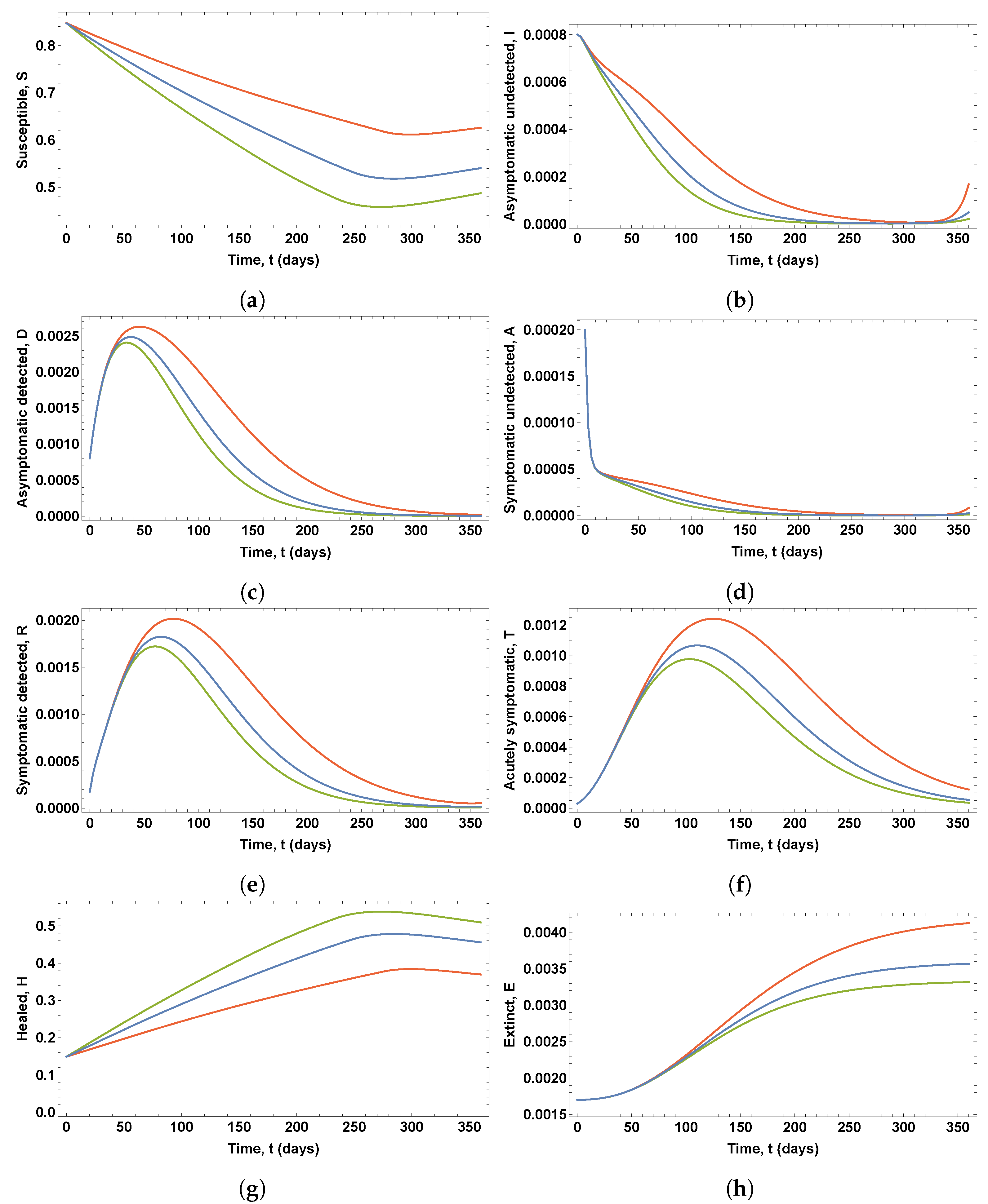
3.2. Sensitivity of the Optimal Policies to the Vaccine Efficacy

Three solutions of the OCP for the SIDARTHE compartmental model (1)–(8) were computed for vaccination scenario 3 assuming vaccine efficacy levels $\varphi = 0.50$, $\varphi = 0.75$, and $\varphi = 0.85$. Moreover, in all these OCPs, the value of the immunity loss rate was set to $\iota = 0.0009$; the lower and upper bounds of the testing rate for the detection of asymptomatic infected people were set to ${\epsilon }_L = 0$ and ${\epsilon }_{\mathbf{u}} = 0.20$, respectively; and the weighting parameters of the objective functional were set to $C_1 = 1,C_2 = 0.1$, and $C_3 = 0.0001$.

Figure 6 shows the optimal control variables obtained in these solutions, which give the optimal vaccination rate and the optimal testing rate for the detection of asymptomatic infected people, whereas Figure 7 shows the eight state variables associated with these optimal control policies.

It can be seen in Figure 6 that changes in vaccine efficacy lead to solutions that show significant variations in both the optimal vaccination rate and the optimal testing rate for the detection of asymptomatic infected people. The lower the efficacy of the vaccine, the longer the duration of the period of growth of the vaccination rate and the shorter the duration of the peak value of the vaccination rate profile. Similarly, the lower the vaccine efficacy, the longer the duration of the period of testing at the maximum rate.

It can be seen in Figure 7 that changes in vaccine efficacy lead to solutions that show noticeable variations in the proportion of susceptible, infected, diagnosed, recognized, threatened, healed, and deceased people. Lower values of the vaccine efficacy imply a delay in the peaks of the curves of diagnosed, recognized, and threatened people, which also reach higher peak values. For example, the percentage of threatened people on the worst day rises to 0.1243%, 0.1067%, and 0.0977%, for vaccine efficacy levels 50%, 75%, and 95%, respectively. Thus, the number of threatened subjects on a single day could increase by approximately 12500 people as the vaccine efficacy varies from 95% to 50% in a country like Spain. Moreover, in these solutions, the percentage of healed people would be 38.41%, 47.83%, and 53.82%, for vaccine efficacy levels 50%, 75%, and 95%, respectively. Finally, a new increase in the proportion of asymptomatic undetected people can be observed in Figure 7b at the end of the period under consideration, which could imply a new outbreak of the disease.

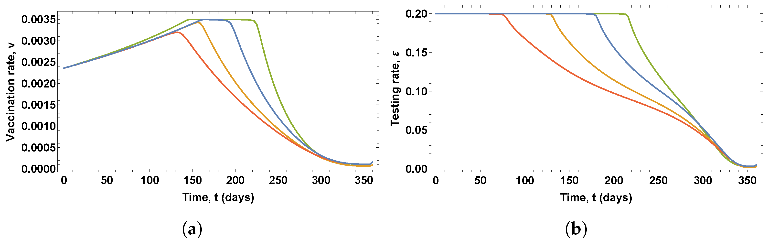
3.3. Sensitivity of the Optimal Policies to the Weighting Parameters of the Objective Functional

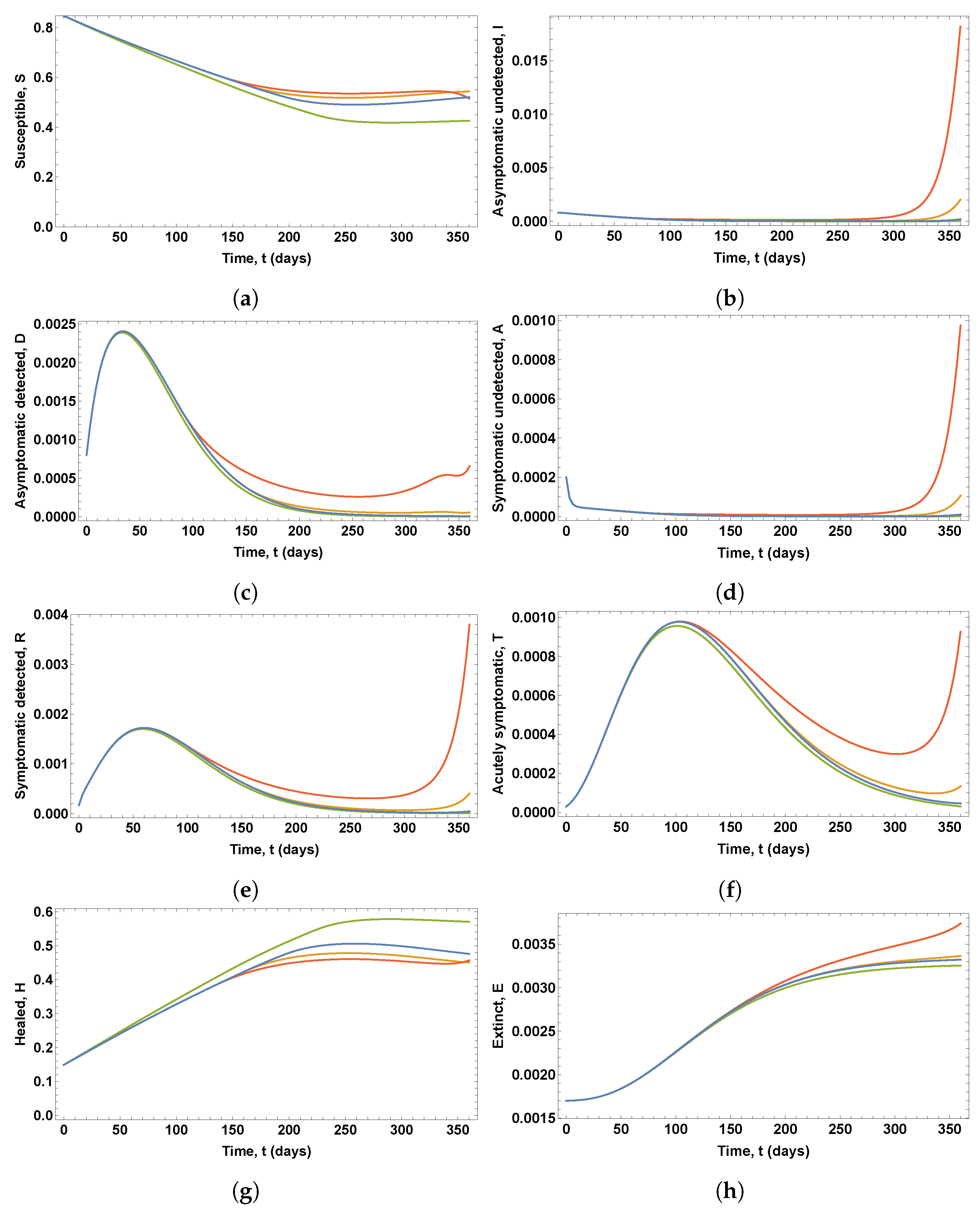
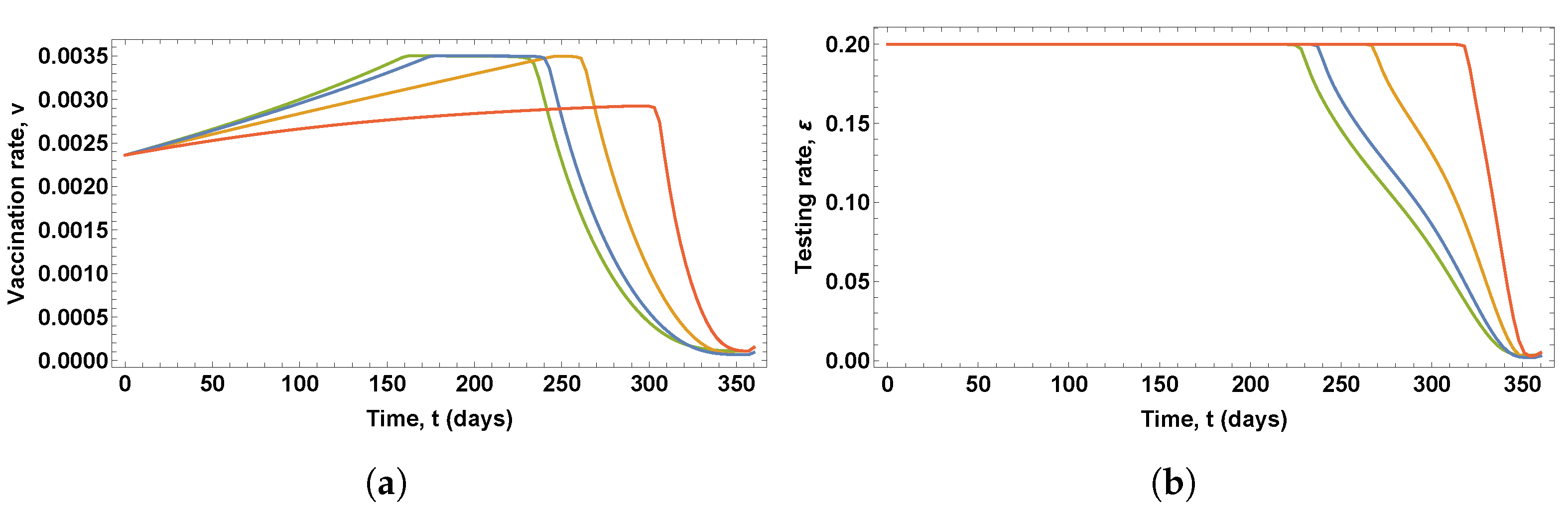
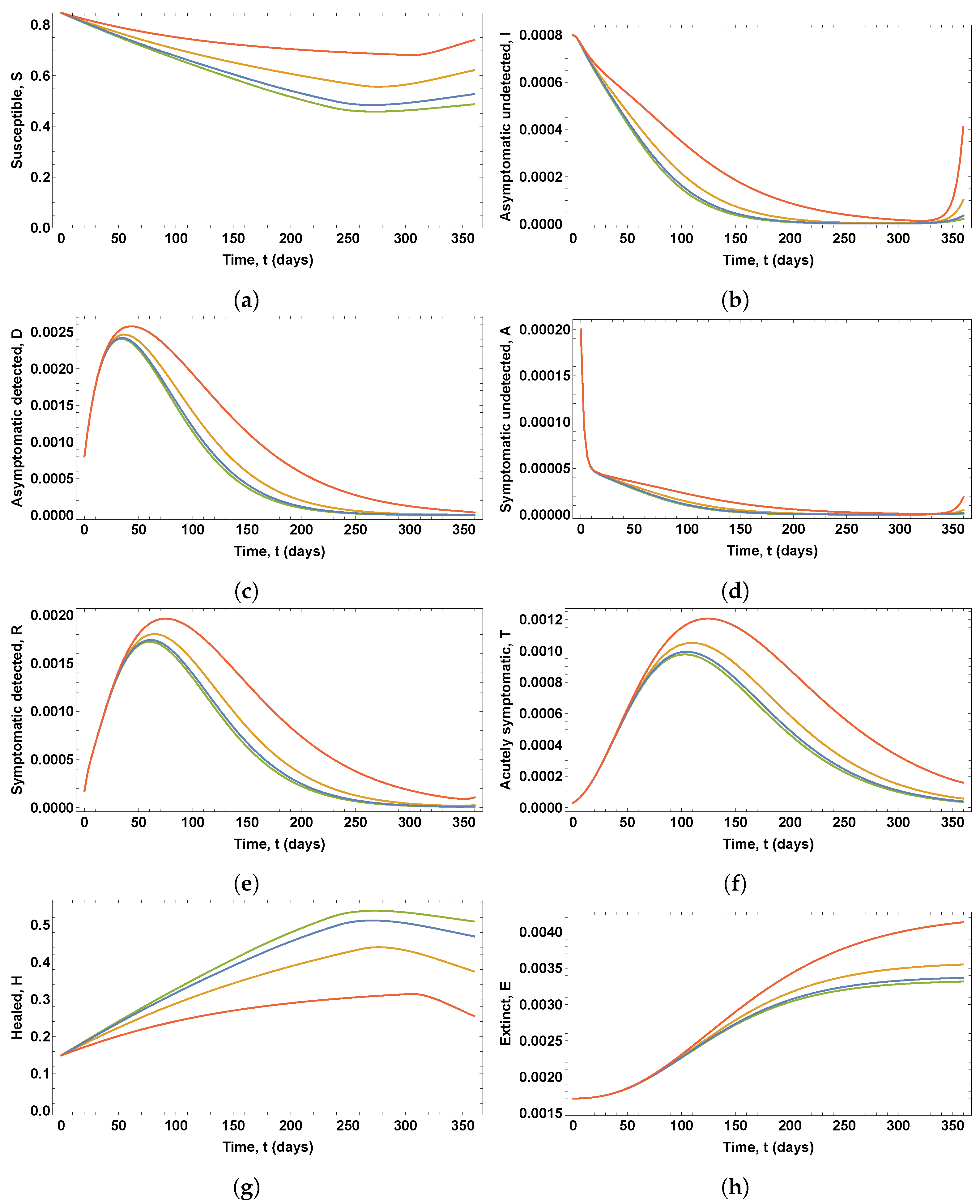
Several solutions of the OCP for the SIDARTHE compartmental model (1)–(8) have been computed using vaccination scenario 3 with different values of the weighting parameters of the objective functional, assuming that $C_1 = 1$, $C_2 = 0.1$, and $C_3 = 0.0001$ are the reference set of weighting parameters. Moreover, in all these OCPs, the value of the immunity loss rate was set to $\iota = 0.0009$, the lower and upper bounds of the testing rate for the detection of asymptomatic infected people were set to ${\epsilon }_L = 0$ and ${\epsilon }_{\mathbf{u}} = 0.20$, respectively, and the vaccine efficacy level was set to $\varphi = 0.95$.

Figure 8 shows the optimal control variables obtained in the solutions of four OCPs, in which four different values of the parameter $C_1$ were used, namely, $C_1 = 0.001$ (red), $C_1 = 0.01$ (orange), $C_1 = 0.1$ (blue), and $C_1 = 1$ (green). Figure 9 shows the eight state variables associated with these optimal control variables.

It can be seen in Figure 8 that changes in parameter $C_1$ lead to noticeable variations in both the optimal vaccination rate and the testing rate for the detection of asymptomatic infected people. The lower the values of parameter $C_1$, the longer the duration of the peak value of the vaccination rate profile and the longer the duration of the period of testing at the maximum rate. However, as shown in Figure 9, only for $C_1 = 0.001$ and $C_1 = 0.01$ are there significant changes in the proportions of infected, diagnosed, ailing, recognized, threatened, and deceased people, with a new outbreak occurring.

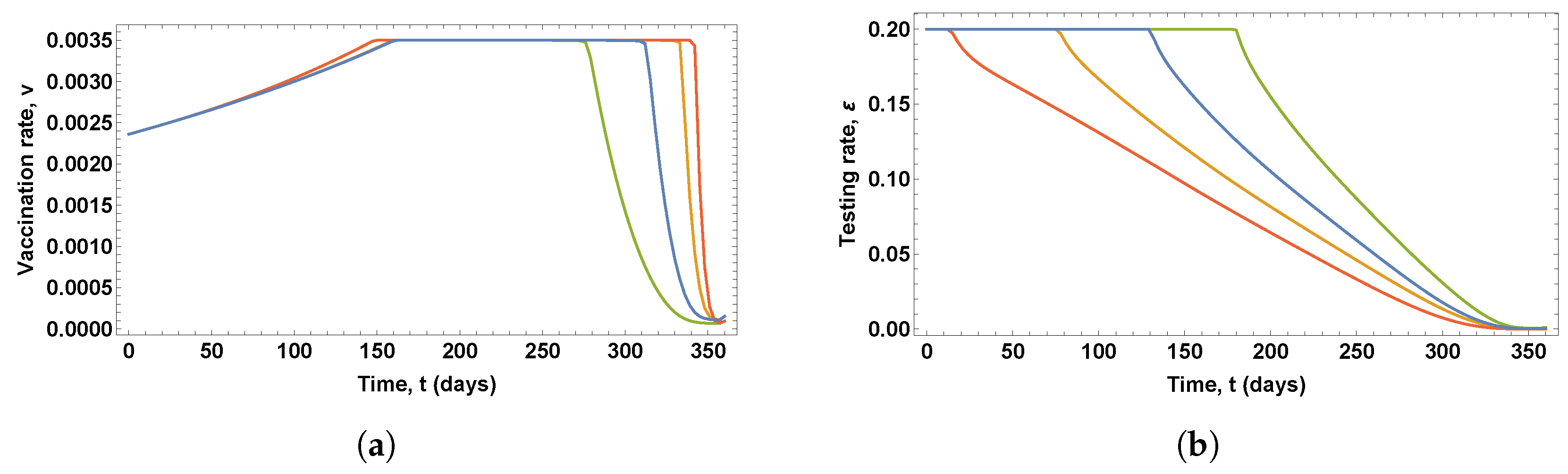
Figure 10 shows the optimal control variables and the corresponding proportions of susceptible and healed people obtained in the solutions of four OCPs, in which four different values of the parameter $C_2$ were used, namely, $C_2 = 0.001$ (red), $C_2 = 0.01$ (orange), $C_2 = 0.1$ (blue), and $C_2 = 1$ (green). It can be seen that changes in the parameter $C_2$ led to noticeable variations in the optimal vaccination rate, whereas slight differences can be observed in the optimal testing rate for the detection of asymptomatic infected people. The lower the values of parameter $C_2$, the longer the duration of the period of vaccination at a maximum rate. However, very similar proportions of infected, diagnosed, ailing, recognized, threatened, and deceased people were obtained in these solutions. Significant differences were only found in the proportions of susceptible and healed people due to the different vaccination profiles, as shown in Figure 10c,d.

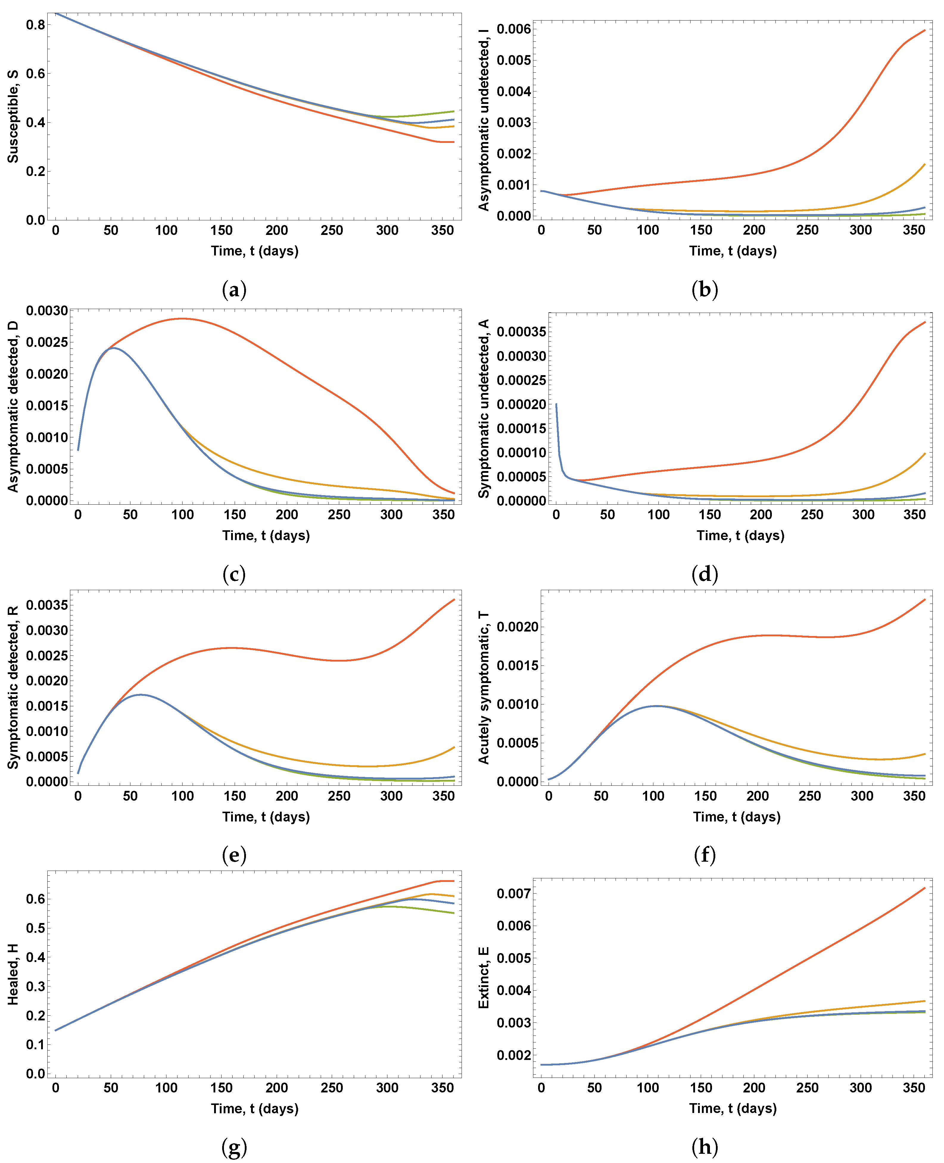
Figure 11 shows the optimal control variables obtained in the solutions of four OCPs, in which four different values of the parameter $C_3$ were used, namely, $C_3 = 1$ (red), $C_3 = 0.1$ (orange), $C_3 = 0.01$ (blue), and $C_3 = 0.001$ (green). Figure 12 shows the eight state variables associated with these optimal control policies.

It can be seen in Figure 11 that changes in parameter $C_3$, in general, lead to significant variations in both the optimal vaccination rate and the optimal testing rate for the detection of asymptomatic infected people. The lower the values of parameter $C_3$, the shorter the duration of the period of vaccination at the highest rate and the longer the duration of the period of testing at the maximum rate.

As shown in Figure 12 noticeable increases in the proportions of infected, diagnosed, ailing, recognized, threatened, and deceased people resulted for $C_3 = 1$. This is due to the low optimal testing rate obtained in the solution, even though the duration of the period of vaccination at the maximum rate is longer than in the rest of the cases. Similarly, due to the low testing rate, new increases in the proportions of infected and ailing people at the end of the period under consideration are shown for $C_3 = 0.1$, which could imply a new outbreak of the disease.

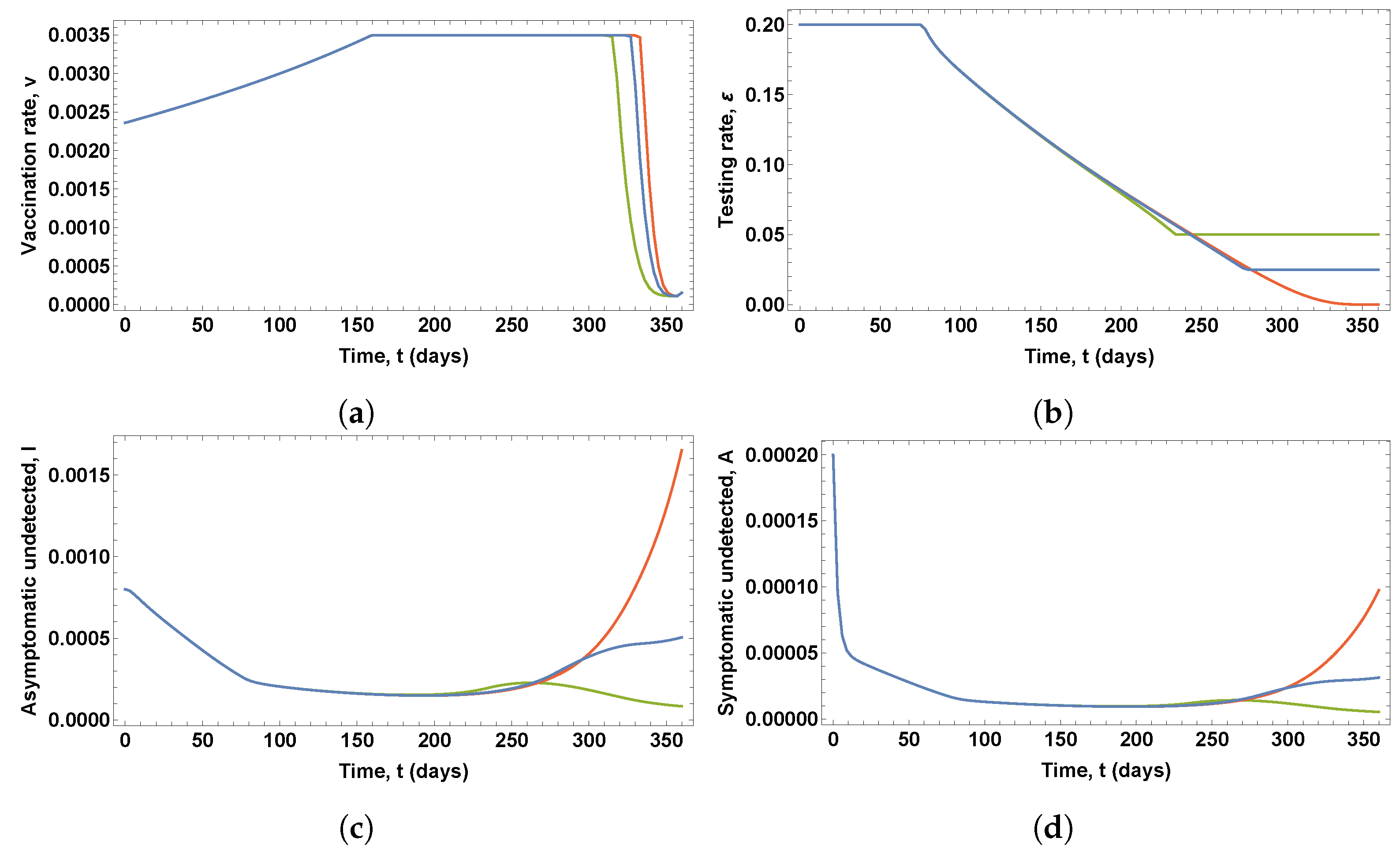
3.4. Sensitivity of the Optimal Policies to the Lower Bound of the Testing Rate

Three solutions of the OCP for the SIDARTHE compartmental model (1)–(8) have been computed for vaccination scenario 3, in which the weighting parameters of the objective functional were set to $C_1 = 1,C_2 = 0.1$, and $C_3 = 0.1$, the value of the immunity loss rate was set to $\iota = 0.0009$, and the vaccine efficacy level was set to $\varphi = 0.95$.

Figure 13 shows the optimal control variables and the corresponding proportions of infected and ailing people obtained in the solutions of three OCP, in which three different values of the lower bound of the testing rate for the detection of asymptomatic infected people were used, namely, ${\epsilon }_L = 0$ (red), ${\epsilon }_L = 0.025$ (blue), and ${\epsilon }_L = 0.05$ (green); and the upper bound was set to ${\epsilon }_{\mathbf{u}} = 0.20$.

Very similar proportions of susceptible, diagnosed, recognized, threatened, healed, and deceased people were obtained in these solutions. However, significant differences can be observed in the proportions of infected and ailing people due to the different values of the lower bound ${\epsilon }_L$, as shown in Figure 13c,d. Therefore, increasing the lower bound ${\epsilon }_L$ may prevent new increases in the proportions of symptomatic and asymptomatic people, and thus a potential new outbreak may be avoided.

3.5. Sensitivity of the Optimal Policies to the Immunity Loss Rate

Four solutions of the OCP for the SIDARTHE compartmental model (1)–(8) have been computed for vaccination scenario 3 assuming immunity loss rates $\iota = 0.0009$, $\iota = 0.0014$, $\iota = 0.0028$, and $\iota = 0.0056$. Moreover, in all these OCPs, the vaccine efficacy level was set to $\varphi = 0.95$; the lower and upper bounds of the testing rate for the detection of asymptomatic infected people were set to ${\epsilon }_L = 0$ and ${\epsilon }_{\mathbf{u}} = 0.20$, respectively; the weighting parameters of the objective functional were set to $C_1 = 1,C_2 = 0.1$, and $C_3 = 0.0001$.

Figure 14 shows the optimal control variables obtained in these solutions, which give the optimal vaccination rate and the optimal testing rate for the detection of asymptomatic infected people, whereas Figure 15 shows the eight state variables associated with these optimal control policies.

It can be seen in Figure 14 that similar optimal vaccination and testing rates were obtained for immunity loss rates $\iota = 0.0028$ and $\iota = 0.0056$. However, significant differences can be observed for immunity loss rates $\iota = 0.0009$ and $\iota = 0.0014$. The higher the immunity loss rate, the longer the duration of the period of growth of the vaccination rate and the shorter the duration of the peak value of the vaccination rate profile. Similarly, the higher the immunity loss rate, the longer the duration of the period of testing at the maximum rate.

It can be seen in Figure 15, that there are slight variations in all the state variables for immunity loss rate $\iota = 0.0028$, which imply a delay in the peaks of the curves of diagnosed, recognized, and threatened people and higher peak values. Moreover, new increases in the proportions of symptomatic and asymptomatic undetected people can be observed, and thus a potential new outbreak might occur. Notice that these same variations are more noticeable for immunity loss rate $\iota = 0.0056$, which imply significant delays and higher peak values.

4. Discussion

Regarding the input controls used in the formulation of the corresponding OCPs, some previous works have considered only non-pharmaceutical interventions against COVID-19, such as isolation of the population [27]; quarantining, hospitalization interventions, and treatment of infected people [15,17]; isolation, quarantine, and public health education [16], sensitization, quarantine, diagnosis, and monitoring and psychological support [19]; public health education, treatment of infected individuals, and health care measures for asymptomatic infectious people [21]; and use of face-masks, hand sanitizer, and social distancing; treatment of patients and active screening with testing; and prevention against recurrence and reinfection of people who have recovered [26]. Fewer works have focused on pharmaceutical measures, such as allocation of the treatment [18] and vaccine administration [20,23,24,25]. In this paper, both kinds of measures, pharmaceutical and non-pharmaceutical, have been considered as the input controls of the proposed OCPs. More specifically, various vaccination and testing policies for controlling COVID-19 have been proposed for three vaccination scenarios represented by different constraints related to vaccine availability and administration. Their impacts on the spread of this disease have also been compared.

Regarding the objective functional used in the formulation of the corresponding OCPs, some previous works have considered just a single optimality criterion, such as the minimization of the number of infected people [18], the number of deaths [27], or the years of life lost due to premature mortality and the years lost due to disability [23]. Some other works have considered and compared several optimality criteria, such as minimizing the number of new infections, the number of deaths, the life years lost, and the quality-adjusted life years lost due to death [20], or minimizing the number of symptomatic infections, the number of deaths, the number of cases requiring non-ICU hospitalization, and the number of cases requiring ICU hospitalization [24]. Finally, other works have combined different optimality criteria with the cost of applying the controls, such us the number of infected people [16,21], the numbers of exposed and infected people [26], or the numbers of susceptible, infected, exposed, and asymptomatic people [15,17,19]. Similarly, in this paper, a combination of the proportions of threatened and deceased people together with the cost of vaccination of susceptible people and detection of asymptomatic infected people were taken as the objective functional to be minimized.

The results of the numerical experiments indicate that different vaccination policies are recommended for the three proposed scenarios, whereas similar testing policies were obtained for scenarios 1 and 2. In scenario 1, the maximum vaccination rate is applied from the very first day and then gradually decreases to 0.0015, when vaccine stocks are exhausted. Similarly, in scenario 2, the maximum vaccination rate is applied from the very first day. However, the optimal vaccination rate gradually decreases at a higher rate until it reaches zero at the end of the time period under consideration, when vaccine supplies are not exhausted. The optimal vaccination policy for scenario 3 differs considerably from those found for the other two scenarios. The solution for scenario 3 implies a vaccination policy in which the vaccination rate gradually increases, reaches the maximum level for 3 months, and then gradually decreases to zero. Despite the differences in the optimal vaccination strategies, scenarios 1 and 2 provide the same proportions of infected, threatened, and deceased people, but different proportions of susceptible and recovered people. Moreover, the proportions of infected, threatened, and deceased people are significantly higher for scenario 3, which supports the hypothesis that early control interventions help to reduce the effects of the pandemic.

The sensitivity analysis of the optimal solutions revealed that a decrease in vaccine efficacy might result in considerable increases in the proportions of threatened and deceased people. Moreover, changes in the values of the weighting parameters of the objective functional related to the proportion of threatened and deceased people and the testing rate for the detection of asymptomatic infected people might lead to a new outbreak, despite the vaccination policy. However, this potential new outbreak could be prevented by setting a large enough threshold on the testing rate, which supports the idea that, in addition to vaccination, the testing for the detection of asymptomatic infected people might be crucial to overcoming the COVID-19 pandemic. Finally, similar results are obtained when the duration of the immunity is assumed to be 2 or more years, whereas slight changes appear when the duration of the immunity is assumed to be 1 year. These changes become noticeable when the duration is assumed to be 6 months, in which a significant increase in the proportion of threatened and deceased people is observed, and the beginning of a new outbreak.

Notice that, at the time this article was written, October 2021, 78% of the Spanish population had been vaccinated, which represents a considerably higher percentage than that provided by any of the three proposed strategies. These differences are due to several factors. First, at the beginning of the summer of 2021 the vaccination plan underwent a drastic change due to the reception of a much greater number of vaccines than that initially scheduled and the use of large vaccination facilities in addition to the public health centers. Secondly, almost 8% of the population has been vaccinated with a single dose of the Janssen vaccine. Moreover, a percentage of the recovered people, those under 65, has also been vaccinated with a single dose, although this percentage has not been reported yet by the Spanish Government, since the eighth version of the vaccination strategy against COVID-19 in Spain has not been updated since June 2021. Lastly, due to the increase in the stock of vaccines that occurred during the summer of 2021, which was actually a scenario with unlimited resources, the Spanish vaccination policy was maximizing the number of vaccinations, unlike the strategies proposed in this work, which, under the hypothesis of limited resources, minimized combinations of the number of vaccinations, the number of tests, and the numbers of threatened and deceased people. Moreover, in the last few months, the ENE-COVID study has not been updated, and therefore the percentage of Spanish people who might have lost their immunity is unknown.

5. Conclusions

Various strategies for preventing the spread of SARS-CoV-2 have been proposed in this paper, based on the premise that a limited supply of effective COVID-19 vaccines and tests are available. These strategies have been devised for a variety of vaccination scenarios that include vaccine supply and administration constraints, and their impacts on COVID-19 transmission have been assessed. The strategies have been determined through the numerical solutions of optimal control problems of a compartmental model that allows social distancing policies, vaccine efficacy, and reinfection due to waning immunity to be represented. The Hermite–Simpson collocation method has been used to solve the formulated optimal control problems, in which several kinds of algebraic constraints have been used to represent different vaccination scenarios, with the control variables being the vaccination rate and the testing rate for asymptomatic infected people, and with the objective functional being a combination of the proportion of threatened and deceased people together with the cost of vaccination of susceptible people and detection of asymptomatic infected people. According to the findings of the numerical experiments, the proposed optimal control-based approach provides healthcare system administrators with a useful mathematical tool for scheduling vaccination plans and testing strategies to manage the COVID-19 pandemic.