On the Estimation of the Initial Stock in the Problem of Resource Extraction

Abstract

We consider a differential game of non-renewable resource extraction, in which the players do not know the precise value of the resource stock and, thus, have to make an estimate. We define the value of information about the initial stock and give recommendations for the choice of the estimate depending on the parameters of the problem. Further, we consider the situation where the players only know the bounds for the stock of the resource and solve the problem of computing the optimal estimate, such that it minimizes the players’ losses in the worst-case scenario. The analysis allows us to give a simple rule for the choice of the optimal estimate of the resource stock.

1. Introduction

In the problems surrounding resource exploitation—accuracy of information about the initial stock of the resource, or its availability, plays a crucial role, as it influences the future profit of the company [1,2]. To characterize the profit that can be gained based on precise information, one may look at the notion of value of information (VoI). Based on this characteristic, the decision maker may make a decision on whether it is profitable to invest in acquiring more precise information or not. An overview of the recent results devoted to VoI can be found in [3,4], while the papers by [5,6] detail the use of value of information in resource extraction applications.

In this paper, we continue the line of research initiated in [7], and consider the problem of determining the value of information in a continuous time differential game of non-renewable resource extraction with n agents (players). Specifically, we compute the value of information on the initial stock of the resource. We first define the value of information for a cooperative scenario and later extend it to the case of the Nash equilibrium solution.

While the computation of the value of information about the initial stock of resource is of great importance, in most situations one does not know how much the initial estimate differs from the exact value. This implies that the exact value of information cannot be computed. In this case, both the initial stock estimate and the value of information are considered within the probabilistic framework, by assuming an a priori probability distribution for the different values of the resource stock. In contrast to that, we present an approach aimed at determining the optimal estimate from purely deterministic considerations.

The rest of the paper is structured as follows. In Section 2, we describe the problem statement, compute the cooperative solution for the considered differential game, and define the normalized value of information. In Section 3, it is shown that, under certain conditions, on the parameters of the system, the previously computed value of information equals the value of information computed for each individual player. Section 4 is devoted to the problem of computing the optimal estimate for the initial resource stock if the only available information is about the lower and upper bounds of the resource stock. Finally, Section 5 concludes the paper.

2. Problem Statement

Below we consider a classical game–the theoretic model of the non-renewable resource extraction. A similar problem was studied by Dockner et al. [8] [Sec. 12.1]. Our problem differs from the one presented in the cited reference in that we consider asymmetric players and finite time-horizon. Moreover, the results related to the computation of the value of information and the optimal estimation of the resource stock are completely new.

Let n players (firms or countries) exploit simultaneously a non-renewable natural resource. We will denote the set of all players by N, i.e., $N=\{1,\dots ,n\}$. Further, $x\left(t\right)$ denotes the state corresponding to the resource stock at time t available to the extraction. The dynamics of the stock is given by the following differential equation with the initial condition $x_0>0$:

$$\dot{x}\left(t\right)=-\sum _{i\in N}{k}_i{u}_i\left(t\right),x\left(t_0\right)=x_0.$$

(1)

Here, $u_i\left(t\right)$ denotes the extraction effort of player i at time t, and the coefficient $k_i$ is used to convert the ith player’s effort into the extraction intensity.

In compliance with the physical nature of the problem, we require that $u_i\left(t\right)\ge 0$ and $x\left(t\right)\ge 0$ for all $t\ge t_0$, and that, if $x\left(t\right)=0$, then the only feasible rate of extraction is $u_i\left(t\right)=0$ for all $i=1,\dots ,n$.

Further, it is assumed that the game is played over a finite time interval $[t_0,T]$, the instantaneous payoff is discounted at a constant rate $r>0$, and the utility function has a constant elasticity of the marginal utility $0<\mu <1$ (see, e.g., Amigues and Moreaux [9]). The latter implies that the marginal utility not only decreases, but its relative change, with respect to the relative change of extraction u, is constant, and is equal to $-\mu$. The parameter $\mu$ is typically interpreted as the measure of risk-aversion, see, e.g., Arrow [10]. The values of $\mu$ within the range $(0,1)$ correspond to the risk averse model of utility.

The objective function of the ith player is defined as

$$J_i(x_0,u_1,\dots ,u_n)=\underset{t_0}{\overset{T}{\int }}{e}^{-rt}\frac{u_i^{1-\mu }\left(t\right)}{1-\mu }dt.$$

(2)

We consider the situation when the game is played in a cooperative mode and the players cooperate in order to achieve the maximum total payoff:

$$\sum _{i\in N}{J}_i(x_0,u_1,\dots ,u_n)=\sum _{i\in N}\underset{t_0}{\overset{T}{\int }}{e}^{-rt}\frac{u_i^{1-\mu }\left(t\right)}{1-\mu }dt.$$

(3)

The optimal open-loop cooperative strategies of players $\overline{u}\left(t\right)=({\overline{u}}_1\left(t\right),\dots ,{\overline{u}}_n\left(t\right))$, $t\in [t_0;T]$ are found from solving the optimization problem:

$$\overline{u}\left(t\right)=\underset{u_1\left(t\right),\dots ,u_n\left(t\right)}{arg\; max}\sum _{i\in N}\underset{t_0}{\overset{T}{\int }}{e}^{-rt}\frac{u_i^{1-\mu }\left(t\right)}{1-\mu }dt.$$

(4)

Note that the problem (1), (4) is well defined for $\mu \in (0,1)$.

The trajectory corresponding to the optimal cooperative strategies $\overline{u}\left(t\right)$ is called the optimal cooperative trajectory and is denoted by $\overline{x}\left(t\right)$.

Following Pontryagin et al. [11], we define the Hamiltonian function as

$$H=\sum _{i\in N}{e}^{-rt}\frac{u_i^{1-\mu }\left(t\right)}{1-\mu }-\psi \left(t\right)\sum _{i\in N}{k}_i{u}_i.$$

Taking into account that $x\left(t\right)\ge 0$ and $u\left(t\right)\ge 0$, the optimal controls ${\overline{u}}_i$ are obtained from the first-order optimality conditions $\frac{\partial H}{\partial u_i}=0$ as

$${\overline{u}}_i\left(t\right)={\left(\frac{e^{-rt}}{\psi \left(t\right)k_i}\right)}^{\frac{1}{\mu }}.$$

Solving the respective canonical system with the transversality condition $\psi \left(T\right)x\left(T\right)=0$, and noting that the adjoint variable is constant, $\psi \left(t\right)=\psi$ and, furthermore, has to satisfy $\psi >0$ so that the expression for ${\overline{u}}_i$ is well-defined, we obtain

$$\psi ={\left[\frac{\mu K\left(e^{\frac{-r{t}_0}{\mu }}-e^{\frac{-rT}{\mu }}\right)}{r{x}_0}\right]}^{\mu },$$

where $K=\sum _{i\in N}{k}_i^{1-\frac{1}{\mu }}$. The optimal state trajectory is thus

$$\overline{x}\left(t\right)=x_0+\frac{x_0\left(e^{\frac{-rt}{\mu }}-e^{\frac{-r{t}_0}{\mu }}\right)}{\left(e^{\frac{-r{t}_0}{\mu }}-e^{\frac{-rT}{\mu }}\right)}.$$

The optimal value of the total payoff then equals

$$\sum _{i\in N}{J}_i(x_0,\overline{u})=\frac{x_0^{1-\mu }}{1-\mu }{\left(\frac{K\mu }{r}\right)}^{\mu }{\left(e^{\frac{-r{t}_0}{\mu }}-e^{\frac{-rT}{\mu }}\right)}^{\mu }.$$

Suppose that the information about the initial resource stock $x_0$ is not available to the players and they overestimate the initial value of the resource stock to be equal to ${\widehat{x}}_0>x_0$. In this case, the controls chosen by the players would have the form

$${\widehat{u}}_i\left(t\right)=\frac{r{\widehat{x}}_0{e}^{\frac{-rt}{\mu }}}{\mu K{k}_i^{\frac{1}{\mu }}\left(e^{\frac{-r{t}_0}{\mu }}-e^{\frac{-rT}{\mu }}\right)},$$

and the trajectory corresponding to these controls is

$$\widehat{x}\left(t\right)=x_0+\frac{{\widehat{x}}_0\left(e^{\frac{-rt}{\mu }}-e^{\frac{-r{t}_0}{\mu }}\right)}{\left(e^{\frac{-r{t}_0}{\mu }}-e^{\frac{-rT}{\mu }}\right)}.$$

Should the players use the controls ${\widehat{u}}_i\left(t\right)$, the resource stock will be exhausted by the time $\widehat{t}<T$, which satisfies

$$e^{\frac{-r{t}_0}{\mu }}-e^{\frac{-r\widehat{t}}{\mu }}=\frac{x_0}{{\widehat{x}}_0}\left(e^{\frac{-r{t}_0}{\mu }}-e^{\frac{-rT}{\mu }}\right).$$

Taking in account that

$$J_i(x_0,\widehat{u})=\underset{t_0}{\overset{\widehat{t}}{\int }}{e}^{-rt}\frac{{\widehat{u}}_i^{1-\mu }\left(t\right)}{1-\mu }dt=\frac{{\widehat{x}}_0^{1-\mu }}{1-\mu }{\left(\frac{\mu }{r}\right)}^{\mu }\frac{x_0{\left(e^{\frac{-r{t}_0}{\mu }}-e^{\frac{-rT}{\mu }}\right)}^{\mu }{k}_i^{1-\frac{1}{\mu }}}{{\widehat{x}}_0{K}^{1-\mu }},$$

(5)

we obtain the following relation:

$$J_i(x_0,\widehat{u})={\left(\frac{x_0}{{\widehat{x}}_0}\right)}^{\mu }{J}_i(x_0,\overline{u}).$$

(6)

It is obvious that the total payoff obtained under the assumption of exact information will never be less than the payoff obtained for imprecise information. To characterize the impact of the accuracy of the available information on the amount of the obtained payoff, we introduce the notion of value of information (VoI).

Definition 1.

The (normalized) value of information in a cooperative game is defined as

$${\mathcal{V}}^C=\frac{{\displaystyle \sum _{i\in N}}{J}_i(x_0,\overline{u})-{\displaystyle \sum _{i\in N}}{J}_i(x_0,\widehat{u})}{{\displaystyle \sum _{i\in N}}{J}_i(x_0,\overline{u})},$$

where ${\sum }_{i\in N}{J}_i(x_0,\overline{u})$ is the total payoff obtained for the exact information about the values of parameters, while ${\sum }_{i\in N}{J}_i(x_0,\widehat{u})$ is the total payoff obtained for an imprecise estimation of the values.

VoI characterizes the maximal amount, the decision maker may wish to pay to achieve the precise information about the value of the parameter of interest. To put it differently, the larger the value of ${\mathcal{V}}^C$ is, the bigger the amount that the decision maker looses when using imprecise information. We have chosen to normalize ${\mathcal{V}}^C$, such that it belongs to the interval $[0,1]$.

Taking into account (6), the value of information about the initial resource stock is computed as

$${\mathcal{V}}^C=\frac{{\widehat{x}}_0^{\mu }-x_0^{\mu }}{{\widehat{x}}_0^{\mu }}=1-{\left(\frac{x_0}{{\widehat{x}}_0}\right)}^{\mu }.$$

In the case when the players underestimate the initial stock, i.e., use the value ${\widehat{x}}_0<x_0$ as an initial condition, the ith player’s payoff is

$$J_i(x_0,\widehat{u})=\frac{{\widehat{x}}_0^{1-\mu }}{1-\mu }{\left(\frac{K\mu }{r}\right)}^{\mu }{\left(e^{\frac{-r{t}_0}{\mu }}-e^{\frac{-rT}{\mu }}\right)}^{\mu }={\left(\frac{{\widehat{x}}_0}{x_0}\right)}^{1-\mu }{J}_i(x_0,\overline{u}).$$

(7)

and the value of information is

$${\mathcal{V}}^C=\frac{x_0^{1-\mu }-{\widehat{x}}_0^{1-\mu }}{x_0^{1-\mu }}=1-{\left(\frac{{\widehat{x}}_0}{x_0}\right)}^{1-\mu }.$$

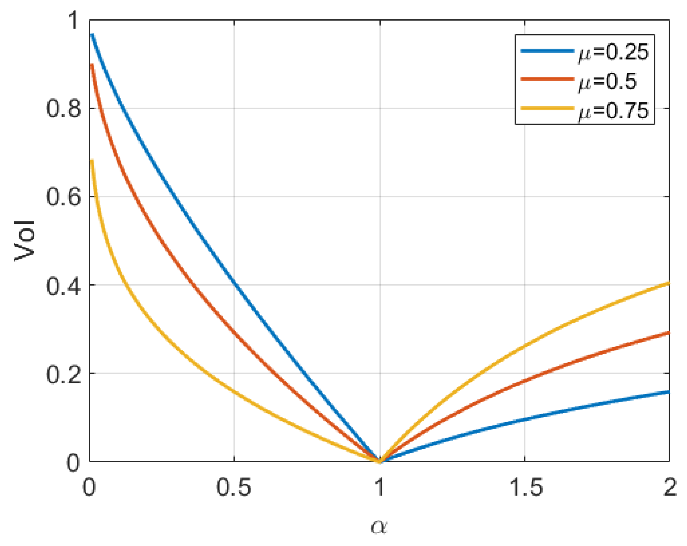
To illustrate the obtained relations, we write ${\widehat{x}}_0$ in terms of $x_0$ as ${\widehat{x}}_0=\alpha x_0$. Here, $\alpha <1$ corresponds to an underestimation of the resource stock, while $\alpha >1$ corresponds to an overestimation thereof. The resulting expression for the value of information thus reads

$$\mathcal{V}=\left\{\begin{array}{cc}1-{\alpha }^{1-\mu },\hfill & \alpha <1,\hfill \\ 0,\hfill & \alpha =1,\hfill \\ 1-{\alpha }^{-\mu },\hfill & \alpha >1.\hfill \end{array}\right.$$

Figure 1 plots the normalized values of information as a function of $\alpha$ for different values of $\mu$.

One can see that if $\alpha =1$, the decision maker possesses the exact information and is not willing to pay anything to improve this knowledge. However, as the information becomes more imperfect (i.e., $\alpha$ deviates from 1), the value of perfect information grows.

One can easily observe that when $\mu$ is small, it is cheaper to overestimate the resource stock, while for larger values of $\mu$, one pays less when underestimating. Let, for instance, $\mu =0.25$. Then an estimation of the available stock of resource to be the half of the actual value would cost approximately $2.5$ times more than if one assumes that the resource stock is twice the actual value (for $\alpha =0.5$, ${\mathcal{V}}^C\approx 0.4$, while for $\alpha =2$, ${\mathcal{V}}^C\approx 0.16$). If, in turn, the value of $\mu$ is close to $\frac{1}{2}$, both overestimation and underestimation result in approximately equivalent losses.

3. Nash Equilibrium

While the notion of VoI was previously introduced for a coalition, one can define value of information for an individual player. In this case, the definition of VoI would be based upon the use of the Nash equilibrium solution. We wish to study the relation between these two notions (cooperative and individual VoI) for the considered problem.

To approach this question, we need to check whether the cooperative solution in this game can be achieved as a Nash equilibrium. It was shown in [8] for an infinite horizon resource extraction game that the answer depends on the values of parameters. Here, we obtain a similar result for the game with finite duration. Similar to the cooperative case, we consider Nash equilibria within the class of open-loop solutions.

Assume that the player i deviates from the optimal cooperative strategy ${\overline{u}}_i\left(t\right)$. Such behavior can be beneficial only if the resource is exhausted by some time $T_i<T$, which means that the deviating player chooses to extract beyond the allocated limit. To illustrate this, suppose that the game ends at the time $T_i>T$. This implies that the ith player extracted less by the time T, which is clearly not optimal. The case $T_i=T$ cannot happen as well, as it would imply that the previously obtained cooperative solution can be improved.

Thus, the player i solves the following optimization problem:

$$\begin{array}{cc}\hfill & \underset{u_i}{max}{J}_i(x_0,{\overline{u}}_1,\dots ,{\overline{u}}_{i-1},u_i,{\overline{u}}_{i+1},\dots ,{\overline{u}}_n),\hfill \\ \hfill & \dot{x}\left(t\right)=-k_i{u}_i\left(t\right)-\sum _{j\ne i}{k}_j{\overline{u}}_j\left(t\right),x\left(t_0\right)=x_0,x\left(T_i\right)=0.\hfill \end{array}$$

(8)

Let, further, ${\tilde{u}}_i$ denote the solution to (8). To find ${\tilde{u}}_i\left(t\right)$, consider the Hamiltonian function for the player i:

$$H_i=e^{-rt}\frac{u_i^{1-\mu }\left(t\right)}{1-\mu }-{\psi }_i\left(t\right)(-k_i{u}_i\left(t\right)-\sum _{j\ne i}{k}_j{\overline{u}}_j\left(t\right)).$$

Solving the respective canonical system we obtain ${\tilde{u}}_i={\overline{u}}_{i}d$, where

$$d=\frac{K\left(e^{\frac{-r{t}_0}{\mu }}-e^{\frac{-rT}{\mu }}\right)-\sum _{j\ne i}{k}_j^{\frac{\mu -1}{\mu }}\left(e^{\frac{-r{t}_0}{\mu }}-e^{\frac{-r{T}_i}{\mu }}\right)}{k_i^{\frac{\mu -1}{\mu }}\left(e^{\frac{-r{t}_0}{\mu }}-e^{\frac{-r{T}_i}{\mu }}\right)}.$$

Then the corresponding value of the i player’s payoff function is

$$J_i(x_0,{\overline{u}}_1,\dots ,{\overline{u}}_{i-1},{\tilde{u}}_i,{\overline{u}}_{i+1},\dots ,{\overline{u}}_n)=\left(e^{\frac{-r{t}_0}{\mu }}-e^{\frac{-r{T}_i}{\mu }}\right){\left(\frac{\mu }{r}\right)}^{\mu }{\left(\frac{x_{0}d}{K\left(e^{\frac{-r{t}_0}{\mu }}-e^{\frac{-rT}{\mu }}\right)}\right)}^{1-\mu }.$$

(9)

The expression (9) attains its maximal value at $T_i=T$ if

$$\mu \ge \frac{1}{K}\sum _{j\ne i}{k}_j^{\frac{\mu -1}{\mu }}$$

(10)

This yields the following.

Lemma 1.

Let the parameters μ and $k_i$ satisfy (10) for each $i\in N$. Then the cooperative solution in this game is a Nash equilibrium.

This result implies that value of information computed on the basis of this particular Nash equilibrium solution will coincide with the value of information obtained for the cooperative case: ${\mathcal{V}}_i^{NE}={\mathcal{V}}^C$ for all $i\in N$.

4. Optimal Estimate for the Initial Resource Stock

Now return to the cooperative game and suppose that the players do not have the information about the exact value of the initial resource stock $x_0$, but they have an a priori estimate that $x_0\in [x_1,x_2]$. Thus the players may decide to agree upon a guess ${\widehat{x}}_0\in [x_1,x_2]$ that would minimize the possible loss in a worst-case scenario. To do so, one solves the following minimax problem:

$$\underset{{\widehat{x}}_0\in [x_1,x_2]}{min}\underset{x_0\in [x_1,x_2]}{max}\left(\sum _{i\in N}{J}_i(x_0,\overline{u})-\sum _{i\in N}{J}_i(x_0,\widehat{u})\right),$$

(11)

where ${\widehat{x}}_0$ is the guess of the initial condition, and $x_0$ is the actual value thereof.

First consider the maximization problem. We rewrite it as

$$\begin{array}{l}\underset{x_0\in [x_1,x_2]}{max}\left(\sum _{i\in N}{J}_i(x_0,\overline{u})-\sum _{i\in N}{J}_i(x_0,\widehat{u})\right)\hfill \\ \hspace{1em}\hspace{1em}\hspace{1em}\hspace{1em}\hspace{1em}\hspace{1em}=max\left\{\underset{x_0\in [x_1,{\widehat{x}}_0]}{max}\left(\sum _{i\in N}{J}_i(x_0,\overline{u})-\sum _{i\in N}{J}_i(x_0,\widehat{u})\right),\right.\\ \hfill \hspace{1em}\hspace{1em}\hspace{1em}\hspace{1em}\hspace{1em}\hspace{1em}\hspace{1em}\hspace{1em}\left.\underset{x_0\in [{\widehat{x}}_0,x_2]}{max}\left(\sum _{i\in N}{J}_i(x_0,\overline{u})-\sum _{i\in N}{J}_i(x_0,\widehat{u})\right)\right\}.\end{array}$$

(12)

Taking into account (6) and (7), we obtain

$$\underset{x_0\in [x_1,x_2]}{max}\left(\sum _{i\in N}{J}_i(x_0,\overline{u})-\sum _{i\in N}{J}_i(x_0,\widehat{u})\right)=Cmax\left((x_1^{1-\mu }-x_1{\widehat{x}}_0^{-\mu }),(x_2^{1-\mu }-{\widehat{x}}_0^{1-\mu })\right),$$

(13)

where $C={\left(\frac{K\mu }{r}\right)}^{\mu }\frac{1}{1-\mu }{\left(e^{\frac{-r{t}_0}{\mu }}-e^{\frac{-rT}{\mu }}\right)}^{\mu }.$

The above optimization problem can be interpreted as a game against nature. For each initial guess ${\widehat{x}}_0$ that the players make, nature chooses the value of $x_0$ that minimizes the total payoff of the players. It turns out that when the admissible range of values for $x_0$ is $[x_1,x_2]$, the best value nature can take would be either $x_1$ or $x_2$, depending on ${\widehat{x}}_0$.

Thus, the best in the sense of loss minimization estimate of the initial condition is given by

$$x_0^{*}=\underset{{\widehat{x}}_0}{arg\; min}\left(max\{(x_1^{1-\mu }-x_1{\widehat{x}}_0^{-\mu }),(x_2^{1-\mu }-{\widehat{x}}_0^{1-\mu })\}\right).$$

The following theorem provides a characterization of the sought-for solution.

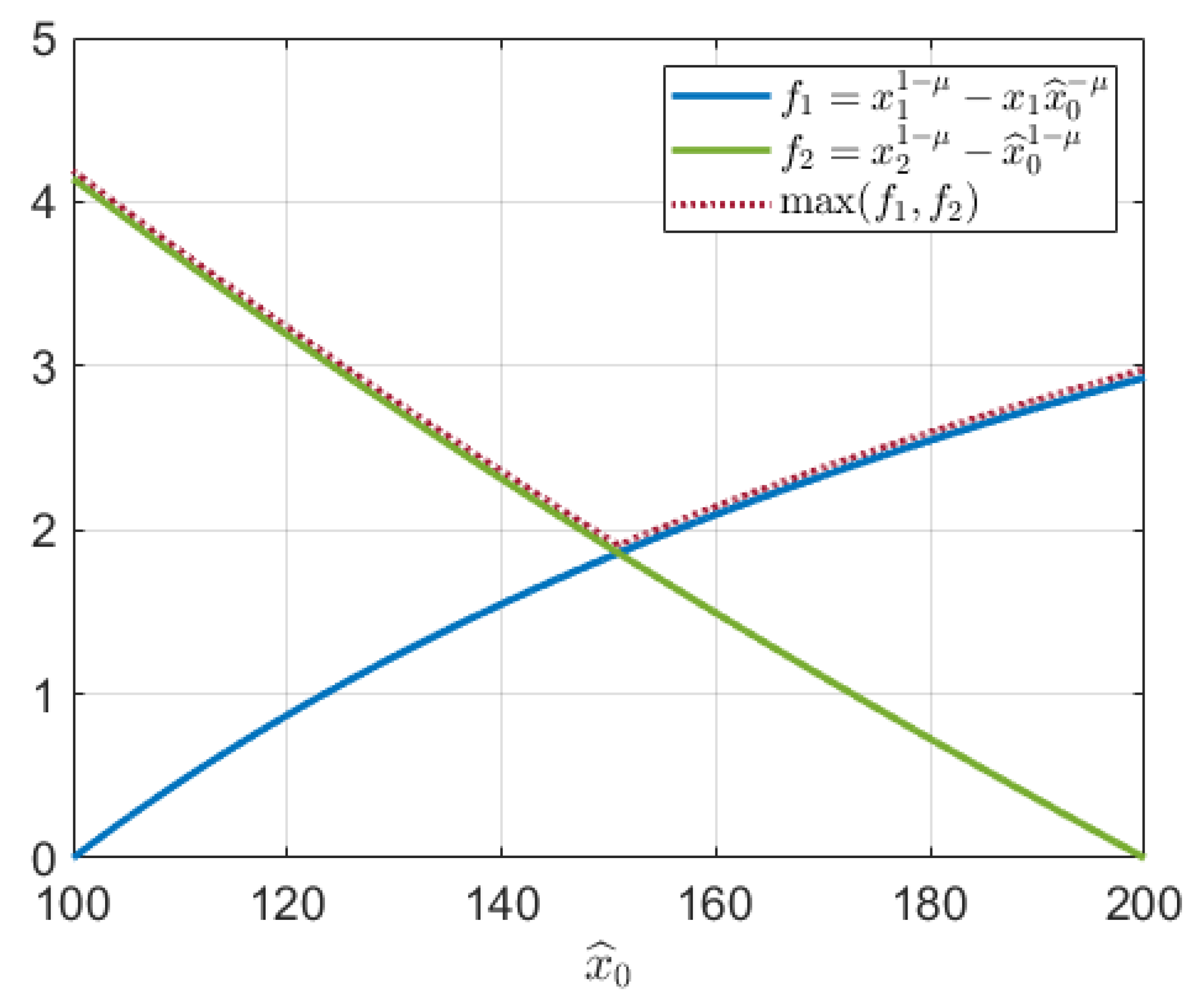
Theorem 1.

The optimal estimate of the initial stock of resource $x_0^{*}$ that solves (11) is given as the solution of the equation

$$x_1^{1-\mu }-x_1{\left(x_0^{*}\right)}^{-\mu }=x_2^{1-\mu }-{\left(x_0^{*}\right)}^{1-\mu }.$$

(14)

Proof. 

Note that over the interval $[x_1,x_2]$, $x_1^{1-\mu }-x_1{\left({\widehat{x}}_0\right)}^{-\mu }$ is an increasing function of ${\widehat{x}}_0$ that changes from 0 to $x_1^{1-\mu }-x_1{\left(x_2\right)}^{-\mu }>0$, while $x_2^{1-\mu }-{\left({\widehat{x}}_0\right)}^{1-\mu }$ is a decreasing function of ${\widehat{x}}_0$ that changes from $x_2^{1-\mu }-x_1^{1-\mu }>0$ to 0.

Thus, we conclude that the graphs of these functions intersect on the interval $[x_1,x_2]$. Therefore, the solution of problem (11) corresponds to the minimum of the upper envelope of both graphs, which is the point of their intersection. □

When $\mu =\frac{1}{2}$, $x_0^{*}$ can be expressed explicitly as

$$x_0^{*}={\left(\frac{\sqrt{x_2}-\sqrt{x_1}+\sqrt{5x_1+x_2-2\sqrt{x_1{x}_2}}}{2}\right)}^2.$$

To illustrate the formulated theorem, we assume the following values of parameters: $x_1=100$, $x_2=200$. Figure 2 demonstrates the graphs of both $x_1^{1-\mu }-x_1{\left({\widehat{x}}_0\right)}^{-\mu }$ and $x_2^{1-\mu }-{\left({\widehat{x}}_0\right)}^{1-\mu }$ as well as their upper envelope for $\mu =\frac{1}{2}$.

Theorem 1 allows us to correct the intuitive rule: if the sought-for value is confined to the interval $[x_1,x_2]$, take the value at the center of the interval. In our case, the “center” of the interval is computed as a solution to a nonlinear equation and its location depends on the value of the elasticity of the marginal utility $\mu$. To analyze this dependence, observe that (14) can be expressed through the fractions as follows:

$${\left(\frac{x_2}{x_1}\right)}^{1-\mu }-1={\left(\frac{x_0^{*}}{x_1}\right)}^{1-\mu }-{\left(\frac{x_0^{*}}{x_1}\right)}^{-\mu }.$$

(15)

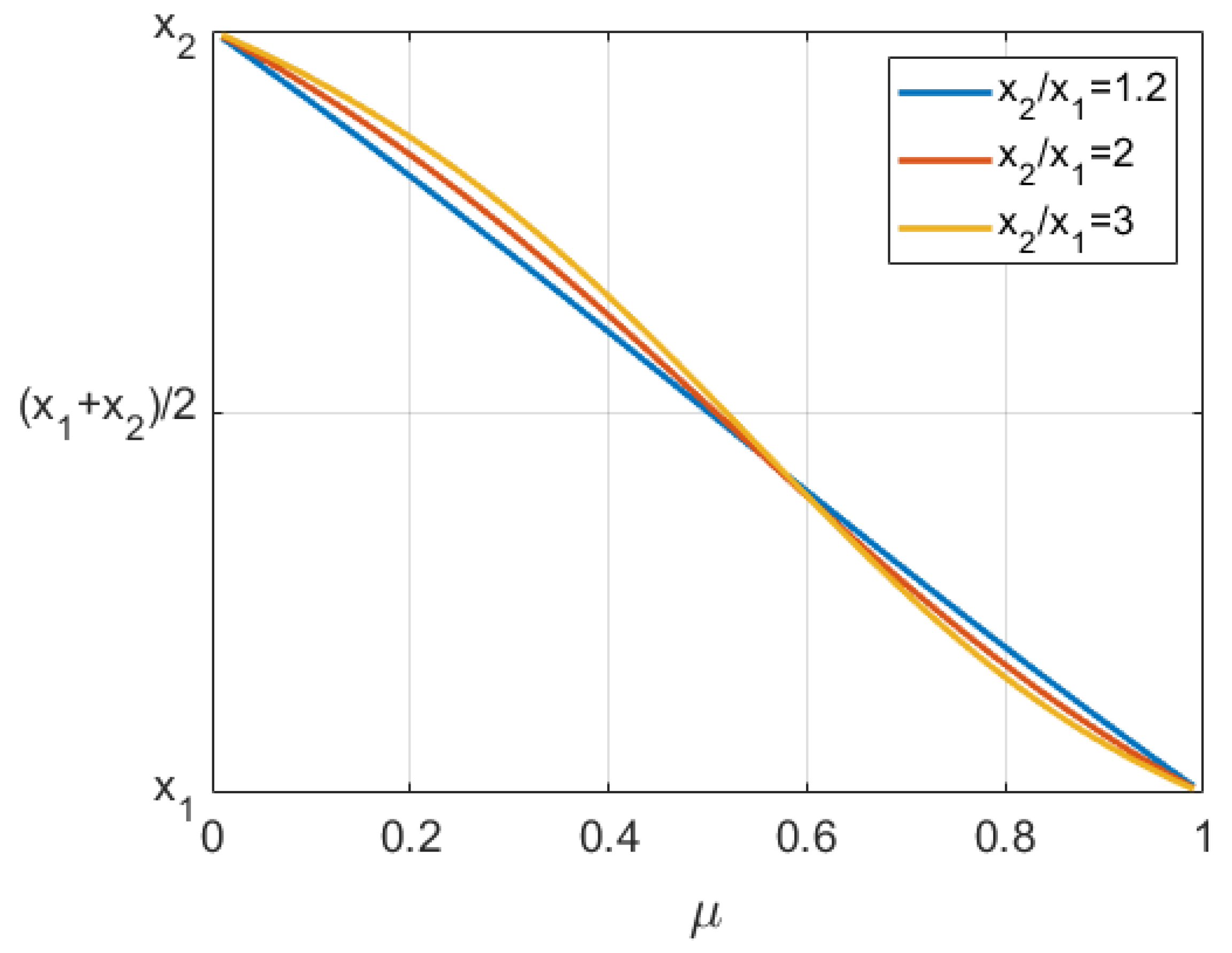
This equation demonstrates that the exact values of $x_1$ and $x_2$ are not substantial, but rather their ratio $x_2/x_1$. The same is true for $x_0^{*}$: Equation (15) specifies it in relation to $x_1$. Figure 3 shows the location of $x_0^{*}$ relative to $x_1$ and $x_2$ for different values of $\mu$ and for different ratios $x_2/x_1$.

One can easily observe that the exact value of the ratio $\frac{x_2}{x_1}$ has no substantial influence on the choice of the estimate $x_0^{*}$. For small values of $\mu$, the estimate of the initial stock should be chosen close to the upper bound $x_2$, while for the values of $\mu$ sufficiently close to 1, one should choose the value of ${\widehat{x}}_0$ that is close to $x_1$. For $\mu =1/2$, the estimate should be taken as the center of the interval, $(x_1+x_2)/2$.

It is instructive to see how the choice of the optimal initial guess affects the value of information. Let $x_1=100$ and $x_2=200$ and assume that the initial guess ${\widehat{x}}_0=x_0^{*}$ is obtained as the solution to (14). In Figure 4, we show the value of information computed for different $\mu$ and for different actual values of the resource stock $x_0$. The points where the value of information is equal to 0 correspond to the case $x_0=x_0^{*}$, while the largest values of ${\mathcal{V}}^C$ are attained at the endpoints of the interval.

5. Conclusions

The carried out analysis can be summarized as follows. If there is no information about the actual resource stock and $\mu$ is small, it is safe to overestimate, while for the values of $\mu$ closer to 1, one should rather underestimate the initial resource stock. If one has an estimation of the bounds of the resource stock, the optimal estimate can be chosen along a straight line that goes from $x_2$ at $\mu \approx 0$ to $x_1$ at $\mu \approx 1$.

While the advantage of the obtained results consists in their deterministic nature, it would be interesting to establish a connection to the results obtained within a probabilistic framework. This will be the subject of our future research.