Distributed Mechanism for Detecting Average Consensus with Maximum-Degree Weights in Bipartite Regular Graphs

Abstract

In recent decades, distributed consensus-based algorithms for data aggregation have been gaining in importance in wireless sensor networks since their implementation as a complementary mechanism can ensure sensor-measured values with high reliability and optimized energy consumption in spite of imprecise sensor readings. In the presented article, we address the average consensus algorithm over bipartite regular graphs, where the application of the maximum-degree weights causes the divergence of the algorithm. We provide a spectral analysis of the algorithm, propose a distributed mechanism to detect whether a graph is bipartite regular, and identify how to reconfigure the algorithm so that the convergence of the average consensus algorithm is guaranteed over bipartite regular graphs. More specifically, we identify in the article that only the largest and the smallest eigenvalues of the weight matrix are located on the unit circle; the sum of all the inner states is preserved at each iteration despite the algorithm divergence; and the inner states oscillate between two values close to the arithmetic means determined by the initial inner states from each disjoint subset. The proposed mechanism utilizes the first-order forward and backward finite-difference of the inner states (more specifically, five conditions are proposed) to detect whether a graph is bipartite regular or not. Subsequently, the mixing parameter of the algorithm can be reconfigured the way it is identified in this study whereby the convergence of the algorithm is ensured in bipartite regular graphs. In the experimental part, we tested our mechanism over randomly generated bipartite regular graphs, random graphs, and random geometric graphs with various parameters, thereby identifying its very high detection rate and proving that the algorithm can estimate the arithmetic mean with high precision (like in error-free scenarios) after the suggested reconfiguration.

1. Introduction

1.1. Theoretical Insight into Wireless Sensor Networks

Several decades ago, it was predicted that embedded networked devices would be massively integrated into our daily lives shortly in order to substitute widespread personal computers [1]. Wireless sensor networks (WSNs), a technology applicable to the low-power measurement and controlling, pose a substantial contribution in completing this magnificent technological shift [1,2]. This technology is formed by tiny affordable autonomous sensor devices (often referred to as sensor nodes/sensors) able to concurrently sense physical quantities of interest, process the sensed information, and wirelessly exchange messages with each other [3,4]. The general architecture of the sensor nodes (see Figure 1) consists of the following five basic components, namely,  [3,5]:

□

Communication device: used to transfer/to receive messages to/from other sensor nodes in the network.

□

Sensors/actuators: their goals are to sense physical quantities from the adjacent environment, to subsequently convert the sensed information into a digital value, and to affect the surroundings.

□

Controller: responsible for processing all the data and for controlling other architecture components.

□

Memory: employed as data storage.

□

Energy source: supplies other components with electric power.

Over the last decades, we have been witnesses to the rapid development of WSNs, mainly due to their high cost-effectiveness and convenience in comparison with traditional wire-based communication technologies [6,7]. As stated in [8,9], the recent progress in wireless communication and micro/nanoelectronic technologies allows WSNs to cooperatively monitor large-scale geographical areas with high accuracy, rapidly process real-time field data, and effectively transmit the relevant information to the end-users through the base station (see Figure 2 for the general architecture of WSNs [10]). In addition, modern sensor nodes present significantly versatile devices, thereby having the ability to sense various dynamically changing physical quantities such as seismic events, light, temperature, humidity, etc. [8,11]. Moreover, the application of WSNs results in other practical benefits such as the possibility to detect tracked events online, simple and fast deployment of the monitoring infrastructure, etc. [12]. Therefore, WSNs (in various modifications) have been significantly attracting the attention of both scientific communities and the industry over recent years [9], thereby finding a wide application in various areas, as shown in Figure 3 [6,7,13,14,15]. In many applications, WSNs can be formed by hundreds to thousands of sensor nodes manually/randomly deployed in hardly accessible and inhospitable terrains; therefore, they are required to reliably operate in the long term despite no technical supervision [3]. So, the algorithms applied in WSNs are intended to be energy efficient and robust to potential failures since the sensor nodes are very prone to numerous negative environmental factors (e.g., temperature, electromagnetic noise, radiation, etc.) [16]. Besides, the measured data can be potentially highly correlated or even duplicated due to a small distance between the sensor nodes distributed over the working area [16]. For these reasons, in many modern WSN-based applications, algorithms for data aggregation are applied to suppress the impact of the mentioned threats on the quality of service (QoS) of the applications executed in WSNs [16].

1.2. Data Aggregation in Wireless Sensor Networks

The term “data aggregation” generally refers to any multi-level data-mining process (executed either manually or by software tools) of integrating a large amount of raw data from independent sources into a report-based summarized form for further statistical processing [17]. The mechanisms for data aggregation are mainly applied to process a data mass that does not provide meaningful information to its owner in the current inconsistent form [5]. As stated in [18], raw data can be classified as either numerical (e.g., temperature, pressure, etc.) or categorical (mineral color, city names, etc.), and the results of data aggregation includes various aggregate functions such as arithmetic mean, extreme, median, mode, range, count, sum, etc. The general architecture of data aggregation in WSNs is shown in Figure 4 [19].

As a literature review shows [5,20,21], the application of data aggregation is beneficial in a wide range of industries, e.g., technical sectors, investments, the travel industry, etc. As further provided, it is usually applied in multi-agent systems whenever the exact value/estimate of some parameter is required to be effectively obtained [17]. As data aggregation poses a multidisciplinary field of science that includes numerous various sub-areas, the author of [17] defines five classification criteria for distinguishing among data-aggregation mechanisms (see Figure 5).

In the following part of this article, we turn the reader’s attention to the fifth classification criterion, i.e., the classification based on the architecture type. In many studies, their authors [22,23,24] have defined two categories of data aggregation in terms of the system architecture, namely, the centralized and the distributed data aggregation schemes (however, as seen in [17], there are also more comprehensive ways of classifying data aggregation mechanisms in terms of the fifth classification criterion). In the centralized scheme, a central node(s) for performing data aggregation is/are present in a network/clusters [22]. As stated in [23], data aggregation in these schemes can be divided into three execution steps:

□

Gathering step: all the sensor nodes in a network/cluster transmit their raw data to a central node [22]. The data are transmitted to this node via wireless channels either directly or by a multi-hop relay [22].

□

Compressing step: in this phase, a central node removes data redundancy caused by high data correlation from the collected data and integrates the raw data into a more applicable summary form.

□

Broadcasting step: the integrated data are distributed among the sensor nodes in the network/clusters in this phase.

Theoretically, the centralized schemes pose an optimal approach, but their implementation in real-world scenarios results in many drawbacks, e.g., a large bandwidth amount, a significant time delay, necessary application of routing mechanisms, high energy requirements, etc. [17]. Moreover, these schemes are generally not appropriate for WSNs with mobile/energy-constrained sensor nodes [22]. Therefore, modern WSN-based applications prefer distributed data aggregation schemes, where no central node for aggregating data is required to be present in a network (unlike the centralized approaches), and the sensor nodes execute data aggregation cooperatively [22]. Besides, data aggregation, in this case, is executed without the need to know the network topology. As stated in [23], the execution of these schemes may be split into two steps:

□

Gathering step: each sensor node broadcasts its local data to its neighbors, i.e., the nodes situated in its transmission range.

□

Compressing step: in contrast to the previous schemes, data compression and integration are executed locally at each sensor node in this phase.

Compared to the centralized approach, these schemes are characterized by decreased communication and computation requirements, higher scalability, higher robustness to potential lapses, etc., thereby finding the usage in a wide range of applications over recent years [25,26,27,28]. As seen in the literature [29,30,31], distributed consensus-based algorithms for data aggregation have been gaining in popularity over the past decades.

1.3. Consensus Problem

Reaching consensus, a sub-field of computer science with a rich history, is understood as a process of achieving agreement in a distributed manner among a group of autonomous entities with non-uniform initial opinions on some abstract fact [22]. As stated in [32], the basic idea of a consensus problem is to share relevant information among entities forming the same system in fault-tolerant ways. The theory of a consensus problem has been widely studied over the last decades, and the distributed consensus algorithms, therefore, find the application in numerous areas (e.g., WSNs, the Internet of Things, cloud computing, etc.) and many various scenarios (e.g., detecting failures, leader election, access to critical resources, clock synchronization, the configuration of a system, etc.) [32,33]. The distributed consensus algorithms pose fault-tolerant and resilient solutions for data aggregation and can guarantee that an accurate and real-time status of the monitored physical quantity is obtained [34]. Therefore, as stated in [34], they are highly recommended for infrastructure-less technologies with severely energy-constrained entities such as WSNs. As the sensor nodes in WSNs are significantly constrained in sensing capabilities, each sensor node is only partially aware of the global status of the observed physical quantity. Therefore, the application of a distributed consensus algorithm ensures that the sensor nodes can easily exchange local information about the observed quantity, update their local observations, and eventually obtain a precise estimate (or even the exact value) about the global status of the observed physical quantity in WSNs [22]. Thus, as found in the literature [35,36,37], distributed consensus algorithms for data aggregation have been becoming a fundamental complement in many WSNs over the past years.

1.4. Our Contribution

In this article, we focus our attention on the average consensus algorithm (AC) with the maximum-degree (MD) weights, which is a distributed iterative consensus scheme for estimating various aggregate functions (namely, the arithmetic mean, the sum, and the network size). More specifically, we deal with AC with MD weights for distributed averaging over bipartite regular graphs, where this algorithm diverges, as identified in [38]. In the first part of our contribution, we provide a spectral analysis of AC with MD weights in bipartite regular graphs. Then, we propose a distributed mechanism for detecting whether or not the algorithm is executed in graphs that are bipartite regular and identify how to properly reconfigure the algorithm in these graphs. This allows ensuring the convergence of AC with MD weights in these critical topologies whereby AC is able to estimate the desired aggregate function after reconfiguration. The proposed distributed mechanism is tested in three scenarios (i.e., the inner states are rounded to either decimals, hundreds, or thousands) over bipartite regular graphs with various degrees as well as in random graphs (RGs) and random geometric graphs (RGGs) with various parameters. In the experimental part, very high detection precision of our mechanism is proven in comprehensive experiments, and it is identified that our proposed mechanism can ensure that the inner states converge to the arithmetic mean although AC with MD weights is executed in bipartite regular graphs. As the literature review shows, our contribution poses a significant novelty compared to other manuscripts from the field, where no similar approach for the mentioned purpose is presented.

1.5. Paper Organization

This article is formatted into seven sections, and several subsections as follows:

□

Related Work (Section 2): this section is concerned with the most recent and most relevant manuscripts from other authors addressing AC or a consensus problem in graphs that are either bipartite regular/bipartite/regular.

□

Theoretical Background (Section 3): this section is divided into two subsections, where the applied mathematical model of WSNs and AC are introduced.

□

Proposal of Mechanism for Detecting Whether Graphs Are Bipartite Regular (Section 4): in this section, which is formed by two subsections, we provide a spectral analysis of AC with MD weights over bipartite regular graphs, propose a novel distributed mechanism for detecting whether a graph representing WSN is bipartite regular or not, and explain how to reconfigure the algorithm after detection.

□

Experimental Section (Section 5): this section consists of two subsections, in which the applied research methodology is introduced, and the experimental results are provided and subsequently discussed. Moreover, it is experimentally identified how to optimally round the inner states for our mechanism.

□

Future Plans (Section 6): here, we reveal what our plans related to the proposed mechanism include.

□

Conclusions (Section 7): in this section, we briefly summarize the contribution presented in this article.

2. Related Work

In this section, we turn the readers’ attention to the most recent and most relevant (in our opinion) studies addressing AC or a consensus problem in graphs that are either bipartite regular/bipartite/regular.

In the first discussed study [38], Schwarz et al. provide an analysis of AC with MD weights/the generalized Metropolis–Hastings algorithm and formulate the sufficient and necessary conditions for convergence of the mentioned algorithms. In the presented research, it is identified that AC with MD weights and the generalized Metropolis–Hastings algorithm with the optimal mixing parameter (as their weight matrices are identical) do not converge in bipartite regular graphs.

The authors of [39] provide some results from the spectral graph theory for graph structures that are regular and connected and determine the lower bound of the ratio: the second smallest Laplacian eigenvalue/the largest Laplacian eigenvalue for Ramanujan graphs. In the presented research, the authors always refer to regular graphs that are non-bipartite. Regular Ramanujan graphs are also extensively addressed in another manuscript [40].

In [41], a heterogeneous diffusion-based communication protocol for improving the convergence rate of AC is proposed. The authors exploit a high rate of heterogeneous diffusion dynamics to improve the performance of AC. The proposed algorithm is (among others) evaluated over bipartite regular graphs, where its convergence rate is greater compared to concurrent approaches.

In [5], it is identified that the best constant weights of a complete graph on an arbitrary number of vertices guarantee the convergence in all its spanning subgraphs without reconfiguration of the edge weights. As a consequence, AC is significantly simplified over WSNs with mobile sensor nodes. Moreover, it is proven in the study that the convergence is also guaranteed in bipartite regular graphs and disconnected graphs the components of which are bipartite regular graphs.

The authors of [42] provide studies on consensus algorithms in triangular regular graphs, where the convergence time, the network coherence, and the maximum communication time delay are analyzed. In the presented study, it is identified that the proposed graph topology is vulnerable to time delay and noise.

The study [43] is concerned with the observability issue in a consensus network with the topology that is either strongly regular or distance regular. The main contribution of the study is that the observability condition does not require that the rank of the observability matrix be computed.

The study [44] is concerned with the effect of the graph size on the convergence rate of AC, and the overall communication costs are examined in regular and irregular graphs. The authors found out that the upper and the lower bound of the convergence rate is only affected by the vertex degree in regular graphs. Besides, it is stated in the article that an increase in the degree ensures a higher convergence rate of the algorithm. The authors furthermore discover a “Magic Number”—the optimum node degree.

In [45], the authors examine the finite-time bipartite consensus problem in multi-agent systems with detail-balanced structure and propose a new weighted signed AC protocol framework.

The study [46] is focused on bipartite consensus in multi-agent systems. It is identified there that bipartite consensus is achieved in multi-agent systems on structurally/vacuously balanced systems in heterogenous signed networks. On the other hand, it is identified in homogeneous signed networks that bipartite consensus forms on all negative bipartite graphs.

The authors of [47] focus their attention on the impact of disturbances on bipartite averaging tracking in multi-agent systems. They propose a non-smooth algorithm to reach the finite-time bipartite averaging tracking. Additionally, two distributed bipartite averaging tracking control algorithms are introduced in this study.

The authors of [48] propose a robust distributed consensus-based algorithm for determining a spectral radius in a network (the largest eigenvalue of the adjacency matrix in this case). The algorithm is based on a log-sum-exp update rule and local communication ensuring that the nodes in a network achieve a consensus on the value of the spectral radius. The authors examine their proposed algorithm in bipartite, non-bipartite, regular, and irregular graphs.

Thus, we can see that only several studies address a consensus problem in graphs that are bipartite regular. Many of the studies provided above (including those that are not provided in this section due to the limited range of the paper) deal with graphs that are either bipartite or regular, and none of them (except for [38]) address AC with MD weights in bipartite regular graphs. In that study, it is, however, only stated that AC with MD weights diverges in this critical topology, a comprehensive analysis of this issue is missing, and no solution of how to overcome it is provided. Thus, our solution poses a significant novelty compared to related studies. See a comparison table (

Table 1. Comparison of our approach to related work—summary.

Paper	Primary Focus of Paper	Applied Graphs of Our Interest
[38]	Formulating the necessary and sufficient convergence conditions for MD weights and the generalized Metropolis–Hastings algorithm	Bipartite regular
[39]	Determining the lower bound for the Laplacian eigenvalues	Ramanujan non-bipartite
[40]	A proposal of an algorithm for finite bit-rate communication	Ramanujan
[41]	A proposal of a diffusion-based communication protocol for improving the convergence rate of AC	Bipartite regular
[5]	A proposal of an algorithm for simplifying AC over mobile systems	Bipartite regular Bipartite regular components
[42]	An analysis of consensus algorithms	Triangular regular
[43]	Addressing the observability issue in a consensus network	Strongly regular Distance regular
[44]	An analysis of AC, discovering the Magic Number	Regular Irregular
[45]	An analysis of the finite-time bipartite consensus problem; a proposal of a new weighted signed AC	Bipartite
[46]	An analysis of the bipartite consensus problem in multi-agent systems	Bipartite
[47]	An analysis of the impact of disturbances on bipartite averaging tracking, a proposal of an algorithm to reach the finite-time bipartite averaging tracking	Bipartite
[48]	A proposal of a distributed algorithm for determining a spectral radius	Bipartite Non-bipartite Regular Irregular
Ours	A proposal of a distributed algorithm for detecting AC with MD weights in bipartite regular graphs, identifying how to reconfigure the mixing parameter	Bipartite regular

) in section Appendix, where the novelty of our study compared to the others is highlighted.

3. Theoretical Background

This section focused on theoretical insight into the topic is split into two subsections, namely:

□

Mathematical Model of Wireless Sensor Networks (Section 3.1): this subsection introduces the graphs of our interest in this article and the tools to describe a network/graph topology.

□

Definition of Average Consensus Algorithm with Maximum-degree Weights (Section 3.2): in this subsection, we provide the definition of AC, its convergence conditions, and the definition of MD weights.

3.1. Mathematical Model of Wireless Sensor Networks

In this article, we consider WSNs formed by homogeneous sensor nodes in terms of the transmission range that can be modeled as undirected simple finite graphs (G = (V(G), E(G))) defined as follows (see an example of an undirected simple finite connected graph (Figure 6)) [5]:

Definition 1. 

An undirected simple finite graph G is a connected/disconnected graph with a finite number of both the vertices and the edges as well as without any multiple edges and loops. Besides, all the edges in G are bidirectional.

The size of WSN is represented by the graph order n, a natural number with a constant value in our analyses/experiments and equal to the cardinality of the vertex set V(G), which contains all the graph vertices (i.e., n = ∣V(G)∣). Each vertex v${}_i$∈V(G), a representative of a particular sensor node, is allocated a unique index, a non-zero natural number i to distinguish the vertices in G from each other (i.e., V(G) = {v${}_1$, v${}_2$, …, v${}_n$ }). Furthermore, the direct connection between two vertices v${}_i$∈V(G) and v${}_j$∈V(G) is represented by the existence of an edge between these two vertices in the edge set E(G) (i.e., e${}_{ij}$∈ E(G)). Thus, the edge set E(G) ⊂V(G)×V(G), whose cardinality determines the graph size, consists of all the graph edges. In what follows, we always refer to an undirected simple finite graph as a graph.

In the literature, one can find many tools to describe the network/graph topologies. Later in this article, we refer to two frequently applied tools, namely, the adjacency matrix A(G) (see (1) for its definition) and the Laplacian matrix L(G) (see (2) for its definition) [49].

$${\left[\mathit{A}\left(G\right)\right]}_{ij}=\left\{\begin{array}{cc}1,\hfill & \mathit{if}{\mathit{e}}_{\mathit{ij}}\in \mathit{E}\left(\mathit{G}\right)\hfill \\ 0,\hfill & \mathrm{otherwise}\hfill \end{array}\right.$$

(1)

$${\left[\mathit{L}\left(G\right)\right]}_{ij}=\left\{\begin{array}{cc}-1,\hfill & \mathit{if}{\mathit{e}}_{\mathit{ij}}\in \mathit{E}\left(\mathit{G}\right)\hfill \\ \phantom{-}{\mathit{d}}_i,\hfill & \mathit{if}i=j\hfill \\ \phantom{-}0,\hfill & \mathrm{otherwise}\hfill \end{array}\right.$$

(2)

As mentioned earlier in this article, we address AC with MD weights over bipartite regular graphs; therefore, let us turn our attention to the two following definitions [50,51]:

Definition 2. 

A graph G is bipartite (sometimes referred to as a bigraph) in the case that its vertex set $\mathit{V}\left(G\right)$ can be partitioned into two disjoint subsets ${\mathit{V}}_1\left(G\right)$ and ${\mathit{V}}_2\left(G\right)$ (sometimes referred to as parts of G) in such a way that any two vertices within the same subset are not adjacent, i.e.,:

$${\mathit{V}}_1\left(G\right)\cup {\mathit{V}}_2\left(G\right)=\mathit{V}\left(G\right)$$

(3)

$${\mathit{V}}_1\left(G\right)\cap {\mathit{V}}_2\left(G\right)=\varnothing$$

(4)

$${\mathit{v}}_i\in {\mathit{V}}_1\left(G\right)\wedge {\mathit{v}}_j\in {\mathit{V}}_1\left(G\right)\Rightarrow {\mathit{e}}_{ij}\notin \mathit{E}\left(\mathit{G}\right)$$

(5)

$${\mathit{v}}_i\in {\mathit{V}}_2\left(G\right)\wedge {\mathit{v}}_j\in {\mathit{V}}_2\left(G\right)\Rightarrow {\mathit{e}}_{ij}\notin \mathit{E}\left(\mathit{G}\right)$$

(6)

In other words, the ends of each edge in G are in different subsets.

Definition 3. 

A graph G is regular in the case that the degree of all the vertices in G is the same. If the degrees are equal to d, G is said to be d–regular (and its size $\mid \mathit{E}\left(\mathit{G}\right)\mid$ = nd).

Thus, bipartite regular graphs, the primary object of our interest, are such graphs that meet both Definitions 2 and 3. In the following text, the value of d is not relevant in the given context (i.e., we refer to regular graphs regardless of the value of d) unless the explicit definition of this value is provided. See Figure 7 for an example of an arbitrary bipartite 2—regular graph with the graph order n = 8.

Later in the article, we also refer to semiregular graphs defined as follows [52]:

Definition 4. 

A graph G is semiregular (also referred to as biregular) in the case that it is bipartite, and all the vertices in the same subset have the same degree. Thus, there are two values of the degrees: ${\mathit{d}}_{{\mathit{V}}_1}$ and ${\mathit{d}}_{{\mathit{V}}_2}$ (we refer to a graph as semiregular only if ${\mathit{d}}_{{\mathit{V}}_1}$≠${\mathit{d}}_{{\mathit{V}}_2}$).

3.2. Definition of Average Consensus Algorithm with Maximum-Degree Weights

In this section, we draw the readers’ attention to AC, a multi-functional distributed iterative scheme for data aggregation in multi-agent systems. The algorithm is mainly designed and frequently applied for distributed averaging (we focus on this functionality in this article) but can also estimate other aggregate functions after minor modifications (the sum and the network size) [5]. In this algorithm, each sensor node initiates its inner state with (for example) a locally measured value and iteratively exchanges it with its neighbors [5]. Besides, it applies the update rule that can be expressed from the global view as the difference Equation (7) in order to determine its inner state for the next iteration [33].

$$\mathbf{x}(\mathit{k}+1)=\mathbf{W}\left(G\right)\mathbf{x}\left(\mathit{k}\right)$$

(7)

Here, x(k) is a variant column vector gathering the inner states of all the sensor nodes in a network (x(0) represents the initial inner states), k is the label of an iteration, and W(G) is a square weight matrix of AC affecting numerous algorithm parameters such as the convergence rate, the robustness to potential threads, the convergence/the divergence of the algorithm, the estimation precision under quantized communication, etc. [5]. As stated in [33], the convergence of AC is only conditioned by the entries of the weight matrix W(G). Thus, the algorithm convergences for weight matrices W(G) with time-unvaried entries (e.g., static error-free networks), provided that all these three convergence conditions are met [53]:

$${\mathbf{1}}^{\mathrm{T}}\mathbf{W}\left(G\right)={\mathbf{1}}^{\mathrm{T}}$$

(8)

$$\mathbf{W}\left(G\right)\mathbf{1}=\mathbf{1}$$

(9)

$$\rho \left(\mathbf{W}\left(G\right)-\frac{1}{\mathit{n}}\mathbf{1}{\mathbf{1}}^{\mathrm{T}}\right)<1$$

(10)

Here, $\rho$(·) is the spectral radius of the provided matrix/vector, 1 is a column all-ones vector, and 1${}^{\mathrm{T}}$ is its transpose [5]. As stated in [33], meeting all these three conditions ensures that the limit provided in (11) exists, i.e., the inner state x${}_i$(k) of each v${}_i$∈ V asymptotically converges to the value of the arithmetic mean (thus, the algorithm is only for determining an estimate of the desired aggregate function and not its exact value).

$$\underset{k\to \infty }{lim}\mathbf{x}\left(\mathit{k}\right)=\underset{k\to \infty }{lim}\mathbf{W}{\left(G\right)}^{\mathit{k}}\mathbf{x}\left(0\right)=\frac{1}{\mathit{n}}\mathbf{1}{\mathbf{1}}^{\mathrm{T}}\mathbf{x}\left(0\right)$$

(11)

One of the most common alternatives of the analyzed algorithm is AC with the Perron matrix (i.e., all the edge weights are equal to the same value determined by the mixing parameter), which is defined as follows [54]:

$$\mathbf{W}\left(G\right)=\mathbf{I}-ϵ\mathbf{L}\left(G\right)$$

(12)

Here, I is an identity matrix, and $ϵ$ represents the mixing parameter. As mentioned earlier in this article, we focus our attention on AC with MD weights, whose weight matrix is Perron and defined as follows [22]:

$${\left[\mathit{W}\left(G\right)\right]}_{ij}=\left\{\begin{array}{cc}\frac{1}{\Delta },\hfill & \mathit{if}{\mathit{e}}_{\mathit{ij}}\in \mathit{E}\left(\mathit{G}\right)\hfill \\ 1-\frac{d_i}{\Delta },\hfill & \mathit{if}\mathit{i}=\mathit{j}\hfill \\ 0,\hfill & \mathrm{otherwise}\hfill \end{array}\right.$$

(13)

Here, the parameter $\Delta$ represents the maximum degree, i.e., the degree of the best-connected vertex in a graph, and d${}_i$ is the degree of a vertex v${}_i$. The parameter $\Delta$ can be easily determined/estimated by applying various techniques (e.g., the max-consensus algorithm, distributed flooding schemes, etc.) whereby AC with MD weights has been finding a wide application in WSNs over the last years [55,56,57].

4. Proposal of Mechanism for Detecting Whether Graphs Are Bipartite Regular

In this section, we provide a spectral analysis of AC with MD weights in bipartite regular graphs, propose a novel distributed mechanism for detecting whether a graph is bipartite regular or not, and examine how to reconfigure the algorithm after successful detection. This section is divided into two parts:

□

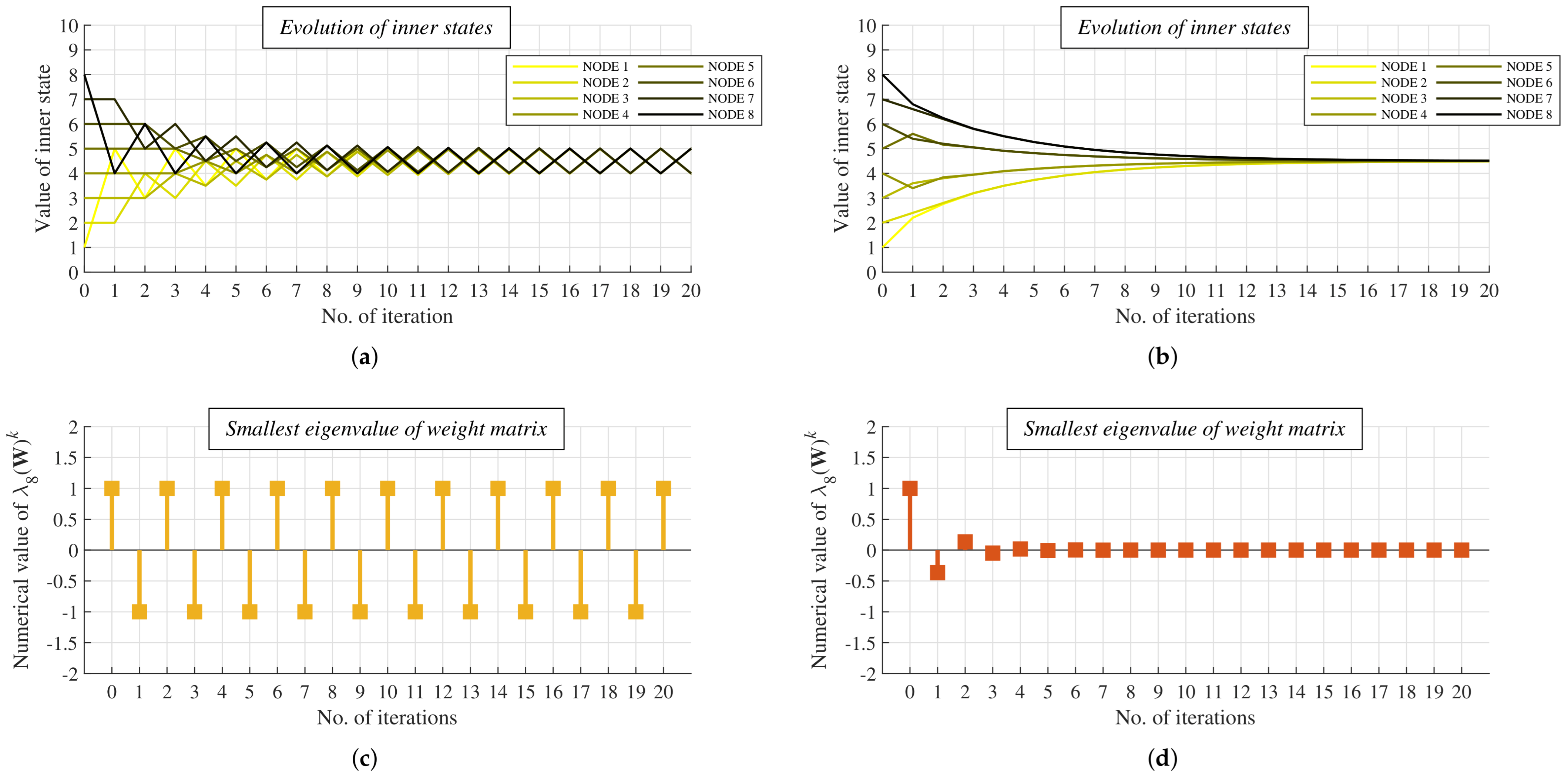
Spectral Analysis of AC with MD weights in Bipartite Regular Graphs (Section 4.1): in this subsection, we analyze the spectrum of the adjacency matrix A(G), the Laplacian spectrum L(G), and the spectrum of the weight matrix W(G), provided AC with MD weights is executed in bipartite regular graphs. We identify in this subsection that only the largest eigenvalue (${\lambda }_1$(W(G)) and the smallest eigenvalue (${\lambda }_n$(W(G)) of the weight matrix W(G) are on the unit circle, causing that the inner states oscillate between two values close to the arithmetic means determined by the initial inner states from each disjoint set, and the sum of all the inner states is preserved at each iteration despite the divergence of the algorithm.

□

Proposed Mechanism for Detecting Bipartite Regular Graphs in Distributed Fashion (Section 4.2): in this subsection, we propose and present five conditions according to which a sensor node can classify whether or not a graph is bipartite regular. Moreover, it is identified in this subsection how to reconfigure the mixing parameter $ϵ$ so that the algorithm converges to the arithmetic mean in bipartite regular graphs after reconfiguration.

4.1. Spectral Analysis of AC with MD Weights in Bipartite Regular Graphs

In this subsection, we present a spectral analysis of AC with MD weights in bipartite regular graphs, as stated above. Specifically, we provide an analysis of the spectrum of the adjacency matrix A(G), the Laplacian spectrum L(G), and the spectrum of the weight matrix W(G) (if AC with MD weights is applied) in bipartite regular graphs. In what follows, we always assume that the eigenvalues of a spectrum are sorted in descending order, i.e.,   

$$SPECTRUM=\{{\lambda }_1(·),{\lambda }_2(·),...,{\lambda }_n(·)\}$$

(14)

Thus, we refer to the largest eigenvalue of the corresponding spectrum as ${\lambda }_1$(·) and the smallest one as ${\lambda }_n$(·).

In our analysis, we firstly focus our attention on Theorem 1, which is concerned with ${\lambda }_1$(W(G)) and ${\lambda }_n$(W(G)) when AC with MD weights is executed in bipartite regular graphs.

Theorem 1. 

Let G be an arbitrary bipartite regular graph with the graph order n. Then, in the case of applying AC with MD weights in G, ${\lambda }_1$(W(G)) and ${\lambda }_n$(W(G)) are always located on the unit circle, taking the values 1 and -1, respectively.

Proof of Theorem 1. 

At first, let us recall that the relation between the Laplacian eigenvalues L(G) and the eigenvalues of the weight matrix W(G) can be expressed as (15), provided that AC with the Perron matrix (12) is applied [33]. Note that the formula (15) is also valid for the weight matrix W(G) of AC with MD weights as the edge weights are the same for each edge in this case ($ϵ=\frac{1}{\Delta }$ in the case of MD weights).

$${\lambda }_i\left(\mathbf{W}\left(G\right)\right)=1-ϵ{\lambda }_{n-i+1}\left(\mathbf{L}\left(\mathit{G}\right)\right)=1,fori=1,2,...,n$$

(15)

Furthermore, by the definition, each Laplacian matrix L(G) is always positive semidefinite L(G) ≽ 0, i.e., all its eigenvalues are non-negative, and one of its Laplacian eigenvalues is always equal to zero (the smallest one is always zero (${\lambda }_n\left(\mathbf{L}\left(\mathit{G}\right)\right)$ = 0) as the matrix is positive semidefinite) [58]. The algebraic multiplicity of the zero eigenvalue is equal to one in the connected graphs, meanwhile, it is greater than one in disconnected graphs. Thus, ${\lambda }_1\left(\mathbf{W}\left(\mathit{G}\right)\right)$ is always equal to one when AC with MD weights is applied since (note that ${\lambda }_1\left(\mathbf{W}\left(\mathit{G}\right)\right)$ is one regardless of the value of the mixing parameter $ϵ$):

$${\lambda }_n\left(\mathbf{L}\left(G\right)\right)=0\Rightarrow {\lambda }_1\left(\mathbf{W}\left(G\right)\right)=1-\frac{1}{\Delta }{\lambda }_n\left(\mathbf{L}\left(G\right)\right)=1$$

(16)

Now, let us focus our attention on ${\lambda }_n\left(\mathbf{W}\left(\mathit{G}\right)\right)$. At first, let us turn our attention to the upper bound of the largest Laplacian eigenvalue ${\lambda }_1\left(\mathbf{L}\left(\mathit{G}\right)\right)$, which can be determined as follows [59]:

$${\lambda }_1\left(\mathbf{L}\left(\mathit{G}\right)\right)\le max\left\{\frac{(d_i+d_j)+\sqrt{{(d_i-d_j)}^2+4{\mathit{m}}_i{\mathit{m}}_j}}{2}:e_{ij}\in \mathbf{E}\left(\mathit{G}\right)\right\}$$

(17)

Here, m${}_i$ represents the average calculated from the degrees of the vertices adjacent to v${}_i$. Moreover, the equality in (17) holds iff a graph is bipartite regular/semiregular [59]. Therefore, the upper bound of ${\lambda }_1(\mathbf{L}$(G)) can be reformulated for bipartite regular graphs as follows [5]:

$${\lambda }_1\left(\mathbf{L}\left(\mathit{G}\right)\right)=2d$$

(18)

As d is also equal to the maximum degree $\Delta$ in regular graphs, Formula (18) can be expressed for these graphs as follows:

$${\lambda }_1\left(\mathbf{L}\left(\mathit{G}\right)\right)=2\Delta$$

(19)

Thus, in the case of AC with MD weights in bipartite regular graphs, ${\lambda }_n$(W(G)) is always equal to minus one since:

$${\lambda }_1\left(\mathbf{L}\left(G\right)\right)=2\Delta \Rightarrow {\lambda }_n\left(\mathbf{W}\left(G\right)\right)=1-\frac{1}{\Delta }{\lambda }_1\left(\mathbf{L}\left(G\right)\right)=-1$$

(20)

   □

In Figure 8, we graphically illustrate the position of both ${\lambda }_1$(W(G)) and ${\lambda }_n$(W(G)) on the unit circle, provided AC with MD weights is applied in bipartite regular graphs.

In the following part, we turn our attention to the other remaining eigenvalues of the weight matrix W(G), provided that AC with MD weights is executed in bipartite regular connected graphs (i.e., {${\lambda }_{n-1}\left(\mathbf{W}\left(\mathit{G}\right)\right)$, ${\lambda }_{n-2}\left(\mathbf{W}\left(\mathit{G}\right)\right)$, …, ${\lambda }_2\left(\mathbf{W}\left(\mathit{G}\right)\right)$}). We do not include disconnected graphs in our analyses since the algorithm cannot estimate the global average in these graphs—the algorithm estimates the local arithmetic mean in each component instead.

Theorem 2. 

In an arbitrary bipartite regular connected graph G with the graph order n, every eigenvalue of the weight matrix W(G) except for ${\lambda }_1\left(\mathit{W}\left(\mathit{G}\right)\right)$ and ${\lambda }_n\left(\mathit{W}\left(\mathit{G}\right)\right)$ is located inside the unit circle, provided AC with MD weights is applied.

Proof. 

As stated in Theorem 1, ${\lambda }_n\left(\mathbf{L}\left(\mathit{G}\right)\right)$ is equal to zero, causing that ${\lambda }_1\left(\mathbf{W}\left(\mathit{G}\right)\right)$ is always one. Additionally, it is identified that ${\lambda }_n\left(\mathbf{W}\left(\mathit{G}\right)\right)$ is minus one as ${\lambda }_1\left(\mathbf{L}\left(\mathit{G}\right)\right)$ is equal to 2$\Delta$ (if AC with MD weights is applied in bipartite regular graphs). The remaining problem to solve is whether the other eigenvalues of the weight matrix W(G) are located on/inside/outside the unit circle if AC with MD weights is applied in the mentioned graphs. In the following part, we identify that all the other eigenvalues of the weight matrix W(G) are inside the unit circle, provided that AC with MD weights is executed in bipartite regular connected graphs. At first, let us turn our attention to how the eigenvalues of the adjacency matrix A(G) and the Laplacian eigenvalues L(G) interlace in regular graphs [39]:

$${\lambda }_i\left(\mathbf{A}\left(G\right)\right)=\Delta -{\lambda }_{n-i+1}\left(\mathbf{L}\left(G\right)\right),\mathrm{for}\mathit{i}=1,2,...,\mathit{n}$$

(21)

$${\lambda }_i\left(\mathbf{L}\left(G\right)\right)=\Delta -{\lambda }_{n-i+1}\left(\mathbf{A}\left(G\right)\right),\mathrm{for}\mathit{i}=1,2,...,\mathit{n}$$

(22)

Therefore, the values of the largest eigenvalue ${\lambda }_1$(A(G)) and the second-largest eigenvalue ${\lambda }_2$(A(G)) of the adjacency matrix A(G) can be determined in regular graphs as follows:

$${\lambda }_1\left(\mathbf{A}\left(G\right)\right)=\Delta -{\lambda }_n\left(\mathbf{L}\left(G\right)\right)$$

(23)

$${\lambda }_2\left(\mathbf{A}\left(G\right)\right)=\Delta -{\lambda }_{n-1}\left(\mathbf{L}\left(G\right)\right)$$

(24)

Analogically for the largest Laplacian eigenvalue ${\lambda }_1$(L(G)) and the second-largest Laplacian eigenvalue ${\lambda }_2$(L(G)), the following can be stated:

$${\lambda }_1\left(\mathbf{L}\left(G\right)\right)=\Delta -{\lambda }_n\left(\mathbf{A}\left(G\right)\right)$$

(25)

$${\lambda }_2\left(\mathbf{L}\left(G\right)\right)=\Delta -{\lambda }_{n-1}\left(\mathbf{A}\left(G\right)\right)$$

(26)

Thus, ${\lambda }_1$(A(G)) is equal to the maximum degree $\Delta$ in regular graphs since:

$${\lambda }_n\left(\mathbf{L}\left(G\right)\right)=0\Rightarrow {\lambda }_1\left(\mathbf{A}\left(G\right)\right)=\Delta -0=\Delta$$

(27)

Subsequently, we show that ${\lambda }_2$(A(G)) is certainly smaller than ${\lambda }_1$(A(G)) in regular connected graphs. However, at first, let us recall that ${\lambda }_2$(L(G)) is greater than zero in connected graphs since the algebraic multiplicity of the zero eigenvalue in the Laplacian spectrum L(G) is always one in the connected graphs, and the Laplacian matrix L(G) is positive semidefinite. Thus, we can state the following:

$$\begin{array}{c}{\lambda }_{n-1}\left(\mathbf{L}\left(G\right)\right)>0\wedge {\lambda }_1\left(\mathbf{A}\left(G\right)\right)=\Delta \Rightarrow {\lambda }_2\left(\mathbf{A}\left(G\right)\right)=\Delta -{\lambda }_{n-1}\left(\mathbf{L}\left(G\right)\right)<{\lambda }_1\left(\mathbf{A}\left(G\right)\right)\end{array}$$

(28)

As stated in [60], the spectrum of the adjacency matrix A(G) is symmetric in bipartite graphs; therefore, the second smallest eigenvalue ${\lambda }_{n-1}$(A(G)) of the adjacency matrix A(G) is always greater than ${\lambda }_n$(A(G)) in bipartite regular connected graphs as:

$$\begin{array}{c}{\lambda }_1\left(\mathbf{A}\left(G\right)\right)=-{\lambda }_n\left(\mathbf{A}\left(G\right)\right)\wedge {\lambda }_2\left(\mathbf{A}\left(G\right)\right)=-{\lambda }_{n-1}\left(\mathbf{A}\left(G\right)\right)\wedge {\lambda }_2\left(\mathbf{A}\left(G\right)\right)<{\lambda }_1\left(\mathbf{A}\left(G\right)\right)\Rightarrow \\ {\lambda }_n\left(\mathbf{A}\left(G\right)\right)<{\lambda }_{n-1}\left(\mathbf{A}\left(G\right)\right)\end{array}$$

(29)

Subsequently, we can prove that ${\lambda }_2$(L(G)) is always smaller than ${\lambda }_1$(L(G)) in bipartite regular connected graphs since:

$$\begin{array}{c}{\lambda }_n\left(\mathbf{A}\left(G\right)\right)<{\lambda }_{n-1}\left(\mathbf{A}\left(G\right)\right)\Rightarrow \Delta -{\lambda }_n\left(\mathbf{A}\left(G\right)\right)>\Delta -{\lambda }_{n-1}\left(\mathbf{A}\left(G\right)\right)\Rightarrow \\ {\lambda }_1\left(\mathbf{L}\left(G\right)\right)>{\lambda }_2\left(\mathbf{L}\left(G\right)\right)\end{array}$$

(30)

Thus, the second smallest eigenvalue ${\lambda }_{n-1}$(W(G)) of the weight matrix W(G) is greater than ${\lambda }_n$(W(G)) and therefore greater than minus one if AC with MD weights is applied in bipartite regular connected graphs as:

$$\begin{array}{c}{\lambda }_1\left(\mathbf{L}\left(G\right)\right)>{\lambda }_2\left(\mathbf{L}\left(G\right)\right)\Rightarrow 1-\frac{1}{\Delta }{\lambda }_1\left(\mathbf{L}\left(G\right)\right)<1-\frac{1}{\Delta }{\lambda }_2\left(\mathbf{L}\left(G\right)\right)\Rightarrow \\ {\lambda }_n\left(\mathbf{W}\left(G\right)\right)<{\lambda }_{n-1}\left(\mathbf{W}\left(G\right)\right)\Rightarrow {\lambda }_{n-1}\left(\mathbf{W}\left(G\right)\right)>-1\end{array}$$

(31)

It is still missing to prove that the second-largest eigenvalue ${\lambda }_2\left(\mathbf{W}\left(\mathit{G}\right)\right)$ of the weight matrix W(G) is always lower than ${\lambda }_1\left(\mathbf{W}\left(\mathit{G}\right)\right)$ (and therefore lower than one) in bipartite regular connected graphs. Thus, we can state the following as the second smallest Laplacian eigenvalue ${\lambda }_{n-1}\left(\mathbf{L}\left(\mathit{G}\right)\right)$ (often referred to as the Fiedler eigenvalue) is always greater than zero in connected graphs:

$$\begin{array}{c}{\lambda }_{n-1}\left(\mathbf{L}\left(G\right)\right)>0\wedge {\lambda }_1\left(\mathbf{W}\left(G\right)\right)=1\Rightarrow \\ {\lambda }_2\left(\mathbf{W}\left(G\right)\right)=1-\frac{1}{\Delta }{\lambda }_{n-1}\left(\mathbf{L}\left(G\right)\right)<{\lambda }_1\left(\mathbf{W}\left(G\right)\right)\end{array}$$

(32)

   □

In the following figures (Figure 9, Figure 10 and Figure 11), we show the spectrum of the adjacency matrix A(G) of a bipartite regular connected and a non-bipartite non-regular connected graph with the graph order n = 8. So, from the Figure 9a,b, we can see that the spectrum of the adjacency matrix A(G) of the bipartite regular connected graph is symmetric in contrast to the non-bipartite non-regular connected graph. Besides, we depict the Laplacian spectrum L(G) of this bipartite regular connected graph (see Figure 10), from which it is seen that ${\lambda }_1$(L(G)) is equal to double the maximum degree $\Delta$. Additionally, it is seen that the difference between the eigenvalues of the adjacency matrix A(G) and the Laplacian eigenvalues L(G) is equal to the maximum degree $\Delta$, which is equal to two in this case. In the last two figures (see Figure 11a,b), the difference in the spectra of W(G) is shown—we can see from the figures that ${\lambda }_n$(W(G)) in the bipartite regular connected graph is equal to minus one, meanwhile, it takes a greater value in the non-bipartite non-regular connected graph (whereby the third convergence condition (10) is met).

In the following lemma, we identify that ${\lambda }_n$(W(G)) is greater than minus one in semiregular graphs, implicating ${\lambda }_n$(W(G)) is only equal to minus one in bipartite regular graphs (since the equality in (17) holds only for bipartite regular/semiregular graphs).

Lemma 1. 

In an arbitrary semiregular graph G with the graph order n, ${\lambda }_n\left(\mathit{W}\left(G\right)\right)$ is always greater than -1, provided that AC with MD weights is applied.

Proof. 

As stated above, the equality in formula (17) holds iff a graph is either bipartite regular or semiregular. In the case of semiregular graphs, formula (17) can be reformulated as follows:   

$${\lambda }_1\left(\mathbf{L}\left(\mathit{G}\right)\right)=\frac{d_{V_1}+d_{V_2}+\sqrt{{(d_{V_1}-d_{V_2})}^2+4d_{V_2}{d}_{V_1}}}{2}=d_{V_1}+d_{V_2}$$

(33)

As mentioned above, we only refer to a graph as semiregular in the case that $d_{V_1}\ne d_{V_2}$, and so:

$$d_{V_1}>d_{V_2}\vee d_{V_1}<d_{V_2}\Rightarrow 2\Delta >d_{V_1}+d_{V_2}$$

(34)

Thus, ${\lambda }_n$(W(G)) is greater than minus one in semiregular graphs since:

$${\lambda }_1\left(\mathbf{L}\left(G\right)\right)=d_{V_1}+d_{V_2}\wedge 2\Delta >d_{V_1}+d_{V_2}\Rightarrow {\lambda }_n\left(\mathbf{W}\left(G\right)\right)=1-\frac{1}{\Delta }{\lambda }_1\left(\mathbf{L}\left(G\right)\right)>-1$$

(35)

   □

In the next part of the article, we focus our attention on Lemma 2, where it is proven why AC with MD weights diverges in bipartite regular connected graphs.

Lemma 2. 

In an arbitrary bipartite regular connected graph G with the graph order n, the mixing parameter ϵ = $\frac{1}{\Delta }$ causes AC with the Perron matrix to diverge in G.

Proof. 

As stated in [33], the third convergence condition (10) can be expressed as follows:

$$\rho \left(\mathbf{W}\left(G\right)-\frac{1}{\mathit{n}}\mathbf{1}{\mathbf{1}}^{\mathrm{T}}\right)=max\{{\lambda }_2\left(\mathbf{W}\left(G\right)\right),-{\lambda }_n\left(\mathbf{W}\left(G\right)\right)\}$$

(36)

So, the application of AC with MD weights ($ϵ$ = $\frac{1}{\Delta }$) results in the divergence of the algorithm in bipartite regular connected graphs as the third convergence condition (10) is not met:

$$\begin{array}{c}{\lambda }_n\left(\mathbf{W}\left(G\right)\right)=-1\wedge {\lambda }_n\left(\mathbf{W}\left(G\right)\right)<{\lambda }_2\left(\mathbf{W}\left(G\right)\right)<1\Rightarrow \\ max\{{\lambda }_2\left(\mathbf{W}\left(G\right)\right),-{\lambda }_n\left(\mathbf{W}\left(G\right)\right)\}=1\end{array}$$

(37)

Therefore, the third convergence condition (10) is broken for the mixing parameter $ϵ$ = $\frac{1}{\Delta }$, and the algorithm diverges in G.    □

In Theorem 3, we identify that the sum of all the inner states is preserved at each iteration even though the algorithm diverges when AC with MD weights is applied in bipartite regular connected graphs. Besides, the inner states oscillate as the number of iterations increases. The algorithm can, therefore, achieve the convergence after our proposed mechanism is applied due to the findings presented in Theorem 3.

Theorem 3. 

In an arbitrary bipartite regular connected graph G with the graph order n, the sum of all the inner states at each iteration is equal to the sum of all the initial inner states (when AC with MD weights is applied) even though the convergence condition (10) is not met. Moreover, the inner states oscillate between two values closed to the arithmetic means determined by the initial inner states from each disjoint subset.

Proof. 

The weight matrix W(G) defined in (13) is a Hermitian matrix, meaning it is equal to its conjugate transpose [61]. Thus, this weight matrix is diagonalizable whereby it can be factorized into a canonical form as:

$$\mathbf{W}{\left(G\right)}^k=\mathbf{Q}{\mathsf{\Lambda }}^k{\mathbf{Q}}^{-1}$$

(38)

Here, Q is a matrix containing all the eigenvectors, and $\mathsf{\Lambda }$ is a diagonal matrix, whose entries are equal to the eigenvalues of the weight matrix W(G). Thus, it is defined as follows:   

$$\mathsf{\Lambda }=\left(\begin{array}{c}{\lambda }_n\left(\mathbf{W}\left(G\right)\right)\\ \phantom{0}& {\lambda }_{n-1}\left(\mathbf{W}\left(G\right)\right)\\ \phantom{0}& \phantom{0}& \ddots \\ \phantom{0}& \phantom{0}& \phantom{0}& {\lambda }_2\left(\mathbf{W}\left(G\right)\right)\\ \phantom{0}& \phantom{0}& \phantom{0}& \phantom{0}& {\lambda }_1\left(\mathbf{W}\left(G\right)\right)\end{array}\right)$$

(39)

By definition, the eigenvectors are orthogonal; therefore, the eigendecomposition (38) can be reformulated as follows [62]:

$$\mathbf{W}{\left(G\right)}^k=\mathbf{Q}{\mathsf{\Lambda }}^k{\mathbf{Q}}^{\mathrm{T}}$$

(40)

Thus, the weight matrix W(G) can be decomposed as follows:

$$\begin{array}{c}\mathbf{W}{\left(G\right)}^k=\mathbf{Q}{\left(\begin{array}{c}{\lambda }_n\left(\mathbf{W}\left(G\right)\right)\\ \phantom{0}& {\lambda }_{n-1}\left(\mathbf{W}\left(G\right)\right)\\ \phantom{0}& \phantom{0}& \ddots \\ \phantom{0}& \phantom{0}& \phantom{0}& {\lambda }_2\left(\mathbf{W}\left(G\right)\right)\\ \phantom{0}& \phantom{0}& \phantom{0}& \phantom{0}& {\lambda }_1\left(\mathbf{W}\left(G\right)\right)\end{array}\right)}^k{\mathbf{Q}}^{\mathrm{T}}=\\ \phantom{\mathbf{W}{\left(G\right)}^k}=\mathbf{Q}\left(\begin{array}{c}{\lambda }_n{\left(\mathbf{W}\left(G\right)\right)}^k\\ \phantom{0}& {\lambda }_{n-1}{\left(\mathbf{W}\left(G\right)\right)}^k\\ \phantom{0}& \phantom{0}& \ddots \\ \phantom{0}& \phantom{0}& \phantom{0}& {\lambda }_2{\left(\mathbf{W}\left(G\right)\right)}^k\\ \phantom{0}& \phantom{0}& \phantom{0}& \phantom{0}& {\lambda }_1{\left(\mathbf{W}\left(G\right)\right)}^k\end{array}\right){\mathbf{Q}}^{\mathrm{T}}\end{array}$$

(41)

At first, let us turn our attention to the case when the convergence conditions (8)–(10) are met. In this case, all the eigenvalues of the weight matrix W(G) except for the largest one are smaller than one in magnitude [33]. Thus:

$$\underset{k\to \infty }{lim}\mathbf{W}{\left(G\right)}^k=\mathbf{Q}\left(\begin{array}{c}0\\ \phantom{0}& 0\\ \phantom{0}& \phantom{0}& \ddots \\ \phantom{0}& \phantom{0}& \phantom{\ddots }& 0\\ \phantom{0}& \phantom{0}& \phantom{\ddots }& \phantom{0}& 1\end{array}\right){\mathbf{Q}}^{-\mathrm{T}}=\mathbf{Q}{\mathbf{Q}}^{-\mathrm{T}}=\frac{{\mathbf{1}}^{\mathrm{T}}\mathbf{1}}{n}$$

(42)

So, it can be seen that each entry of the weight matrix W(G) approaches the value $\frac{1}{n}$. In bipartite regular connected graphs, the entries of the matrix $\mathsf{\Lambda }$ are, however, determined as (43), provided that AC with MD weights is applied:

$${\mathsf{\Lambda }}^k=\left(\begin{array}{c}{(-1)}^k\\ \phantom{0}& {\lambda }_{n-1}{\left(\mathbf{W}\left(G\right)\right)}^k\\ \phantom{0}& \phantom{0}& \ddots \\ \phantom{0}& \phantom{0}& \phantom{\ddots }& {\lambda }_2{\left(\mathbf{W}\left(G\right)\right)}^k\\ \phantom{0}& \phantom{0}& \phantom{\ddots }& \phantom{0}& {\left(1\right)}^k\end{array}\right)$$

(43)

Here, as stated in Theorem 2, each eigenvalue except for the largest and the smallest one is inside the unit circle, i.e., its value in magnitude is smaller than one. Thus, we can state the following:

$$\underset{k\to \infty }{lim}{\lambda }_i\left(\mathbf{W}\left(G\right)\right)=0,fori=2,...,n-1$$

(44)

As further seen, the series ($-1$)${}^k$ is divergent, oscillating between two values as k grows, and the series (1)${}^k$ is equal to one for each k:   

$${(-1)}^k=\left\{\begin{array}{cc}-1,\hfill & fork=1,3,5,...\hfill \\ \phantom{-}1,\hfill & fork=0,2,4,...\hfill \end{array}\right.$$

(45)

$${\left(1\right)}^k=1,fork=1,2,3,...$$

(46)

Thus, the entries in the weight matrix W(G) approach the values given in (47) and (48) (in contrast to the scenario when all the three convergence conditions are met—see Formula (42)) for higher values of k, provided that AC with MD weights is executed in bipartite regular connected graphs.

For even values of k and ∀v${}_i$∈ V(G):

$${\left[W\left(G\right)\right]}_{ij}^k=\left\{\begin{array}{cc}\frac{2}{n},\hfill & if{v}_i\in {\mathbf{V}}_1\left(G\right)\wedge v_j\in {\mathbf{V}}_1\left(G\right)\vee v_i\in {\mathbf{V}}_2\left(G\right)\wedge v_j\in {\mathbf{V}}_2\left(G\right)\vee i=j\hfill \\ 0,\hfill & if{v}_i\in {\mathbf{V}}_1\left(G\right)\wedge v_j\in {\mathbf{V}}_2\left(G\right)\vee v_i\in {\mathbf{V}}_2\left(G\right)\wedge v_j\in {\mathbf{V}}_1\left(G\right)\hfill \end{array}\right.$$

(47)

For odd values of k and ∀v${}_i$∈ V:

$${\left[W\left(G\right)\right]}_{ij}^k=\left\{\begin{array}{cc}0,\hfill & if{v}_i\in {\mathbf{V}}_1\left(G\right)\wedge v_j\in {\mathbf{V}}_1\left(G\right)\vee v_i\in {\mathbf{V}}_2\left(G\right)\wedge v_j\in {\mathbf{V}}_2\left(G\right)\vee i=j\hfill \\ \frac{2}{n},\hfill & if{v}_i\in {\mathbf{V}}_1\left(G\right)\wedge v_j\in {\mathbf{V}}_2\left(G\right)\vee v_i\in {\mathbf{V}}_2\left(G\right)\wedge v_j\in {\mathbf{V}}_1\left(G\right)\hfill \end{array}\right.$$

(48)

Thus, due to (47), (48), the inner state of each vertex ${\mathit{v}}_i\in \mathbf{V}\left(\mathit{G}\right)$ approaches the following values as the number of iterations grows when AC with MD weights is executed in bipartite regular connected graphs. For even values of k and ∀v${}_i$∈ V:

$$x_i\left(k\right)=\left\{\begin{array}{cc}\mathrm{averaged}\mathrm{initial}\mathrm{inner}\mathrm{states}\mathrm{of}\mathrm{all}\mathrm{vertices}\mathrm{from}{\mathbf{V}}_1\left(G\right),\hfill & if{v}_i\in {\mathbf{V}}_1\left(G\right)\hfill \\ \mathrm{averaged}\mathrm{initial}\mathrm{inner}\mathrm{states}\mathrm{of}\mathrm{all}\mathrm{vertices}\mathrm{from}{\mathbf{V}}_2\left(G\right),\hfill & if{v}_i\in {\mathbf{V}}_2\left(G\right)\hfill \end{array}\right.$$

(49)

For odd values of k and ∀v${}_i$∈ V:

$$x_i\left(k\right)=\left\{\begin{array}{cc}\mathrm{averaged}\mathrm{initial}\mathrm{inner}\mathrm{states}\mathrm{of}\mathrm{all}\mathrm{vertices}\mathrm{from}{\mathbf{V}}_2\left(G\right),\hfill & if{v}_i\in {\mathbf{V}}_1\left(G\right)\hfill \\ \mathrm{averaged}\mathrm{initial}\mathrm{inner}\mathrm{states}\mathrm{of}\mathrm{all}\mathrm{vertices}\mathrm{from}{\mathbf{V}}_1\left(G\right),\hfill & if{v}_i\in {\mathbf{V}}_2\left(G\right)\hfill \end{array}\right.$$

(50)

So, it is seen that the inner states oscillate between the values close to those given in Formulas (49) and (50) whereby the sum of all the inner states is preserved in spite of the divergence of the algorithm and equal to the sum determined by the initial inner states of all the vertices in a graph.    □

In the following figures, we show the difference between AC with MD weights in a bipartite regular connected graph and a non-bipartite non-regular connected graph. Namely, we compare the evolution of the inner states (see Figure 12a,b) and the evolution of ${\lambda }_n$(W(G)) (see Figure 12c,d). From the figures, it can be seen that the inner states oscillate as the iteration number grows in the bipartite regular connected graph (Figure 12a) in contrast to the non-bipartite non-regular connected graph (Figure 12b), where the inner states asymptotically converge to the arithmetic mean. From the two other figures, we can see that the value of the examined eigenvalue oscillates between one and minus one in the bipartite regular connected graph (Figure 12c) but approaches zero as the number of iterations increases.

4.2. Proposed Mechanism for Detecting Bipartite Regular Graphs in Distributed Fashion

The subsection is concerned with our proposed mechanism for distributively detecting whether or not a graph is bipartite regular. In all the following parts, we exclude disconnected graphs from our assumptions since AC cannot estimate the global arithmetic mean, as mentioned earlier. As further stated above in this article, it is fundamental to know whether AC with MD weights is executed in bipartite regular as the algorithm diverges in this critical topology (whereby the arithmetic mean from all the initial inner states cannot be estimated). As the literature review provided above shows, there is no similar approach for overcoming this issue even though ignoring it has a fatal impact on AC with MD weights. In this article, we, therefore, introduce a novel distributed mechanism for solving this issue whereby AC with MD weights can be reconfigured during its execution, and the arithmetic mean can be estimated just like in error-free scenarios. The most fundamental benefits of our mechanism can be summarized as:

□

No. 1: the detection is only made according to the difference in inner states of a sensor node whereby no further information (compared to default AC) has to be transmitted. Thus, our proposal is efficient in terms of energy consumption, which is significantly beneficial in energy-constrained technologies such as WSNs. Each node only stores the values of the inner states from previous iterations, based on which it can detect whether or not a graph is bipartite regular.

□

No. 2: as identified in Section 4.1, the sum of all the inner states is preserved although the algorithm diverges. This fact ensures that the inner states can begin to converge to the arithmetic mean (the mean square error (MSE) of the inner states converges to zero) once the detection is completed. Thus, the algorithm does not have to start once again but continues in its execution after reconfiguration.

□

No. 3: the application of our mechanism guarantees a very high detection precision (as shown later in this article) in a short time despite its computational ease.

□

No. 4: it can be applied not only for AC with MD weights but also for the generalized Metropolis–Hastings algorithm with the mixing parameter $ϵ$ = 0 (as their weight matrices are identical [38]). We do not pay further attention to this algorithm in this article due to the limited range of the study. However, analyzing this algorithm is included in our plans.

In this part, we turn our attention to our proposed distributed mechanism (see Algorithm 1 for a pseudo-code of the algorithm if our mechanism is applied). It operates in such a way that each sensor node verifies the validity of five conditions and can then detect whether a graph is bipartite regular or not. The principle of our mechanism is to distributively detect undamped oscillation between the values close to (49) and (50) at each sensor node. The graph is classified by a sensor node (the detection is executed by each sensor node independently) as bipartite regular, provided all these conditions are met. In contrast, the graph is not considered by this node as bipartite regular unless at least one of these five conditions is met. The mentioned five conditions can be mathematically expressed as follows:

$${▿}_2^1{x}_i(k+1)=0$$

(51)

$${▿}_2^1{x}_i\left(k\right)=0$$

(52)

$${\Delta }^1{x}_i\left(k\right)={▿}^1{x}_i(k-1)$$

(53)

$${\Delta }^1{x}_i\left(k\right)\ne 0$$

(54)

$${▿}^1{x}_i(k-1)\ne 0$$

(55)

Here, ${\Delta }_{\Delta \mathit{k}}^1$ and ${▿}_{\Delta \mathit{k}}^1$ are the first-order forward/backward finite difference defined as [63]:

$${\Delta }_{\Delta \mathit{k}}^1{x}_i\left(k\right)=\frac{x_i(k+\Delta \mathit{k})-x_i\left(k\right)}{\Delta \mathit{k}}$$

(56)

$${▿}_{\Delta \mathit{k}}^1{x}_i\left(k\right)=\frac{x_i\left(k\right)-x_i(k-\Delta \mathit{k})}{\Delta \mathit{k}}$$

(57)

The parameter $\Delta$k determines the difference in the values of k, and its value is omitted from the formula if $\Delta$k = 1. As mentioned earlier in this article, the inner states only approach the values (49) and (50); therefore, the values of $x_i(k+\Delta \mathit{k})$, $x_i\left(k\right)$, and $x_i(\Delta \mathit{k}-k)$ have to be rounded for our mechanism (in the experimental part, we analyze how to round these values optimally). In the case that AC with MD weights is executed in bipartite regular graphs, it is assumed that the mixing parameter $ϵ$ of the algorithm is reconfigured after successful detection made by all the nodes. Thus, the remaining issue is how to reconfigure the mixing parameter $ϵ$ to ensure the convergence of the algorithm. In the following lemma, we focus our attention on the values of the mixing parameter $ϵ$ that guarantee the convergence in bipartite regular graphs.

Algorithm 1 AC with MD weights—proposed mechanism is applied

Input: x(0) 1: for$\mathit{k}=0,1,\dots$do 2:     x(k+1) = W(G)x(k) 3:     k = k + 1 4:     if mechanism is applicable at k, and algorithm has not been reconfigured then 5:         for $i=1,2,\dots ,n$ do 6:            if (51), (52), (53), (54), and (55) are true then 7:                v${}_i$ classifies graph as bipartite regular 8:            else 9:                v${}_i$ does not classify graph as bipartite regular 10:            end if 11:         end for 12:     end if 13:     if all vertices have classified graph as bipartite regular at least once during current run of algorithm, and algorithm has not been reconfigured then 14:         mixing parameter $ϵ$ is reconfigured according to Lemma 3 15:     end if 16: end for      Output: x(k) ≈$\overline{\mathbf{x}\left(0\right)}$1

Lemma 3. 

In an arbitrary bipartite regular connected graph G with the graph order n, the mixing parameter 0 < ϵ < $\frac{1}{\Delta }$ ensures that AC with the Perron matrix converges in G.

Proof. 

As stated in Lemma 2, the third convergence condition (10) can be reformulated

$$\rho \left(\mathbf{W}-\frac{1}{\mathit{n}}\mathbf{1}{\mathbf{1}}^{\mathrm{T}}\right)=max\{{\lambda }_2\left(\mathbf{W}\left(G\right)\right),-{\lambda }_n\left(\mathbf{W}\left(G\right)\right)\}$$

(58)

Let us recall that it is further stated in Lemma 2 that the mixing parameter $ϵ$ = $\frac{1}{\Delta }$ results in the divergence of the algorithm in G. Now, let us turn our attention to the value of ${\lambda }_n$(W(G)) if 0 < $ϵ$ < $\frac{1}{\Delta }$:

$${\lambda }_1\left(\mathbf{L}\left(G\right)\right)=2\Delta \wedge 0<ϵ<\frac{1}{\Delta }\Rightarrow {\lambda }_n\left(\mathbf{W}\left(\mathit{G}\right)\right)=1-ϵ{\lambda }_1\left(\mathbf{L}\left(G\right)\right)>-1$$

(59)

Thus, the mixing parameter 0 < $ϵ$ < $\frac{1}{\Delta }$ ensures the third convergence condition (10) is met as:

$$\begin{array}{c}{\lambda }_n\left(\mathbf{W}\left(G\right)\right)>-1\wedge {\lambda }_n\left(\mathbf{W}\left(G\right)\right)<{\lambda }_2\left(\mathbf{W}\left(G\right)\right)<1\Rightarrow \\ max\{{\lambda }_2\left(\mathbf{W}\left(G\right)\right),-{\lambda }_n\left(\mathbf{W}\left(G\right)\right)\}<1\end{array}$$

(60)

Thus, the mixing parameter 0 < $ϵ$ < $\frac{1}{\Delta }$ ensures the convergence in bipartite regular connected graphs. The first and the second conditions (8), (9) are also met, which results from the definition of the matrix (12). □

In Figure 13, we provide a valid example of Lemma 3, i.e., we show the evolution of the inner states and MSE in bipartite regular connected graph—the mixing parameter $ϵ$ is reconfigured from $ϵ$ = $\frac{1}{\Delta }$ to either 0 < $ϵ$ < $\frac{1}{\Delta }$ and $ϵ$ > $\frac{1}{\Delta }$ at k = 13. From the figures, we can see that the inner states oscillate before the reconfiguration of the mixing parameter $ϵ$ in both the cases (see Figure 13a,b). Once the mixing parameter $ϵ$ is reconfigured, the inner states converge to the arithmetic mean in the first case, meanwhile, the algorithm diverges for $ϵ$ > $\frac{1}{\Delta }$. Besides, it is observed that MSE approaches a constant value before the algorithm is reconfigured. After the reconfiguration, MSE decreases as the number of the iteration grows for $ϵ$ < $\frac{1}{\Delta }$ in contrast to $ϵ$ > $\frac{1}{\Delta }$, when MSE increases with the growth of k.

5. Experimental Section

This section, where the precision of our proposed mechanism is evaluated, is divided into two subsections, namely:

□

Applied Research Methodology (Section 5.1): in this subsection, we introduce the applied research methodology (i.e., specification of the executed experiments, the used graph types, the analyzed scenarios, and how the initial inner states are generated) and the metrics applied to evaluate the performance of our mechanism.

□

Experiments and Discussion (Section 5.2): this part consists of three sets of figures (22 figures overall) demonstrating how precisely our mechanism can detect whether or not AC with MD weights is executed over a graph that is bipartite regular and how MSE of the inner states evolves when our mechanism is applied. Subsequently, a discussion about observable phenomena is provided.

5.1. Applied Research Methodology

In this subsection, we turn the reader’s attention to the applied research methodology and the metrics for performance evaluation. All the experiments, the results of which are presented in Section 5.2, were carried out in Matlab2018b (Producer: MathWorks, Location: Natick, Massachusetts, USA). In this article, WSNs were modeled as either random bipartite regular graphs, RGs (that are not bipartite regular), or RGGs (that are not bipartite regular)—all with the graph order n = 30.

In the case of bipartite regular graphs, we varied the value of the parameter d in order to generate graphs of various connectivity. Its greater value ensures that the graph connectivity is higher. In our experiments, this parameter took these values:

□

d = {2, 3, 4, 5, 6, 7, 10, 15}

For each value of d, 100 unique graphs were generated; therefore, the precision of our mechanism was tested over 800 bipartite regular graphs overall. In these graphs, it was verified how precisely our mechanism can detect that a graph where AC with MD weights is executed is bipartite regular.

The next applied graph type are RGs generated in such a way that an edge between each pair vertices exists with the probability p [64]. Its higher values cause graphs to be better connected. In the experiments, its value is equal to the following values:

□

p = {5%, 10%, 15%, 20%}

Again, 100 unique graphs were generated for each p; therefore, our mechanism was tested over 400 RGs overall. The purpose of these graphs is to evaluate the precision of how our mechanism can detect that AC with MD weights is not executed in bipartite regular graphs.

The last graph type applied in our experiments is RGGs, where each vertex is placed uniformly at random in a free position over a square working area [64]. Once all the vertices are placed, two vertices are linked to one another, provided that their distance is not greater than their transmission radius [64]. In our experiments, we assumed two categories of these graphs, namely, densely and sparsely connected—see Figure 14 for their representatives. Different connectivity was ensured by changing the value of the transmission radius. For each connectivity, 100 graphs with a unique topology were generated whereby the performance of our mechanism was evaluated over 200 RGGs. Just like in the case of RGs, it was also tested in these graphs how precisely our mechanism detects that AC with MD weights is not executed in bipartite regular graphs.

As the inner states only approach the values provided in (49), (50), their values had to be rounded for our mechanism (note that the rounded values were only used by our mechanism—AC exploits non-rounded values). Therefore, we defined and mutually compared three scenarios that differ from each other as follows:

□

Scenario 1: the inner states exploited by the proposed mechanism are rounded to decimals.

□

Scenario 2: the inner states exploited by the proposed mechanism are rounded to hundreds.

□

Scenario 3: the inner states exploited by the proposed mechanism are rounded to thousands.

As mentioned earlier in this paper, we examined how precisely our proposed mechanism can detect that AC with MD weights is executed in both bipartite regular graphs and graphs that are not bipartite regular as well as the impact of the application of the mechanism on MSE of the inner states. The experimental part in this article is, therefore, divided into three parts:

□

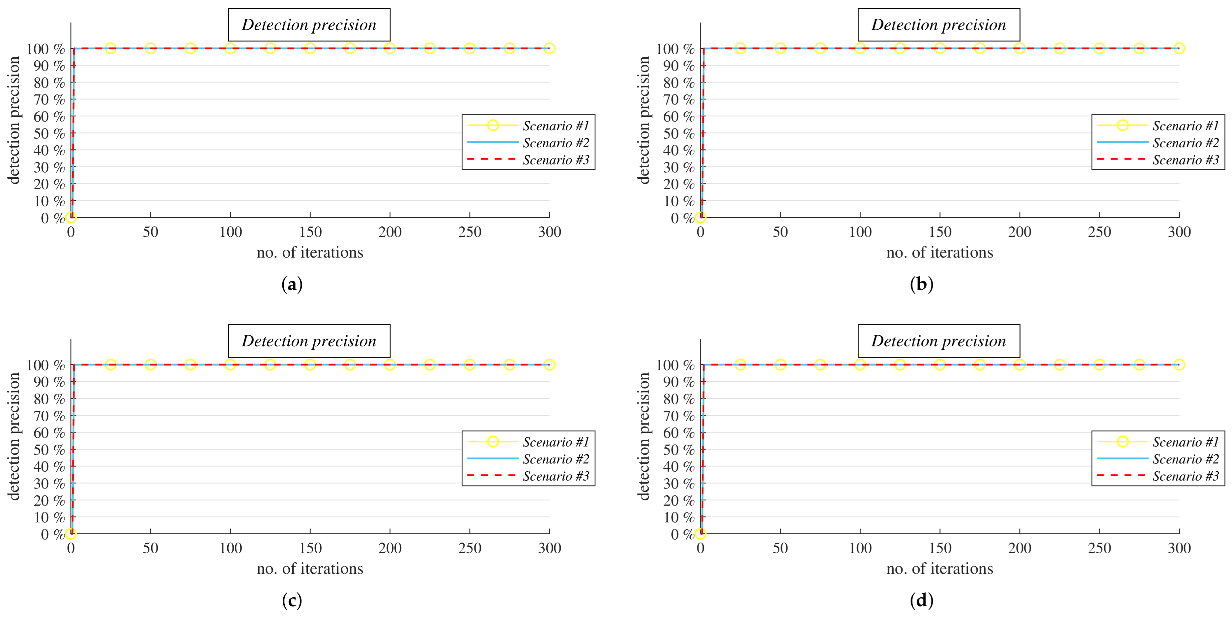
Analysis I. (see Figure 15): in this part, we test how precisely our mechanism can detect that AC with MD weights is executed over bipartite regular graphs. To evaluate the performance of the proposed mechanism, we analyzed how many sensor nodes correctly detect (at each iteration) that a graph is bipartite regular (an incorrect detection means that the mechanism detects that the graph is not bipartite regular in this case). The detection precision is expressed as the ratio: the correct detections in the whole network at an iteration/all the executed detections in the whole network at the same iteration, and this precision is expressed in percentages. In the figures shown below, we only depict the precision averaged over 100 graphs for each d.

□

Analysis II. (see Figure 16 and Figure 17): the second part is concerned with how precisely the mechanism that detects that AC with MD weights is executed over graphs that are not bipartite regular. The performance is just like in the previous analysis evaluated by applying the ratio: the correct detections in the whole network at an iteration/all the detections in the whole network at the same iteration—expressed in the percentages again. However, in this case, a correct detection means that our mechanism classifies that a graph is not bipartite regular. In this part, AC with MD weights was evaluated over both RGs and RGGs, as mentioned above. Like in Analysis I., we only depict the detection precision averaged over 100 graphs for each p and each connectivity of RGGs, respectively.

□

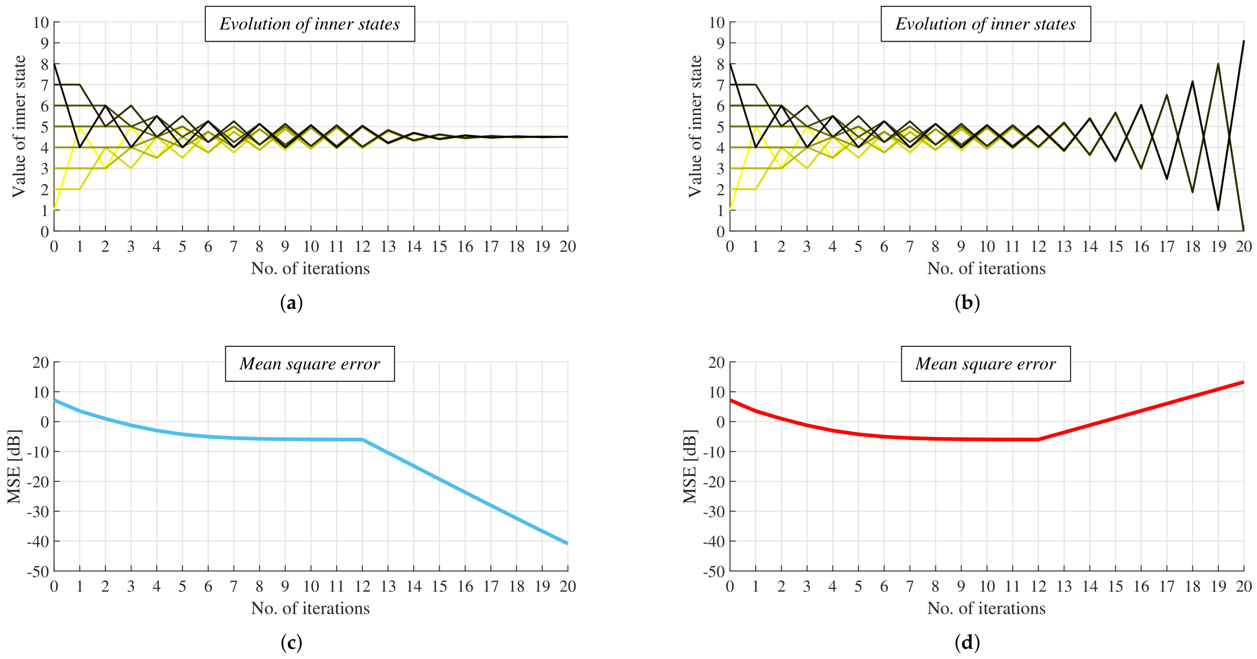
Analysis III. (see Figure 18): the last analysis provided in this article is focused on MSE-based analysis, i.e., we examined how MSE evolves when our mechanism is applied. The mixing parameter $ϵ$ is reconfigured to the value equaling 0.9$\frac{1}{\Delta }$ immediately after all the sensor nodes detect that a graph is bipartite regular. The goal of this analysis was to demonstrate that AC with MD weights can converge in bipartite regular graphs when our proposed mechanism is applied and to identify in which scenario high performance of the algorithm is achieved (thus, we found out how to round the inner states optimally). To quantify the deviation of the inner states from the arithmetic mean, we applied MSE over iterations defined as follows [65]:

$$\mathrm{MSE}\left(k\right)=\frac{1}{\mathit{n}}\sum _{i=1}^{\mathit{n}}{\left(x_i\left(k\right)-{\mathbf{1}}^{\mathrm{T}}\frac{\mathbf{x}\left(0\right)}{\mathit{n}}\right)}^2$$

(61)

Again, averaged MSE over 100 graphs for each d is only depicted in the figures.

Furthermore, the initial inner states in each experiment are independent and identically distributed (IID) random values (representatives of independent local measurements) of the standard Gaussian distribution, which can be expressed as follows:

$${\mathit{x}}_{\mathit{i}}\left(0\right)\sim \mathit{N}(0,1),\phantom{.}for\phantom{.}\forall {\mathit{v}}_{\mathit{i}}\in \mathbf{V}$$

(62)

5.2. Experiments and Discussion

In this section, we present the experimental results from three extensive analyses and provide a discussion about observable phenomena.

The first analysis (Analysis I) was concerned with how precisely our mechanism can detect that AC with MD weights is executed in bipartite regular graphs without any knowledge about the graph topology. As mentioned earlier in this article, we examined three scenarios and tested our mechanism over randomly generated bipartite regular graphs with various d. From the results shown in Figure 15, it was seen that the precision of our mechanism grows with an increased iteration number for each value of d and in each examined scenario (with a few exceptions). As further seen from the figures, the precision was low for lower values of iterations but rapidly grew with an increase in the iteration number. Besides, it was seen that the growth rate increased with an increase in d. For a higher number of iterations, it was observed that the precision of our proposed mechanism was equal to or greater than 87% in Scenario 1, 96% in Scenario 2, and even more than 98.7% in Scenario 3. On the other hand, its precision did not exceed the value equal to 97% at any iteration in Scenario 1 in contrast to the two other scenarios, in which the precision of 100% was observed at numerous iterations. It can be further seen from the presented results that rounding the inner states to decimals ensures very high detection precision for a lower number of iterations compared to the cases of rounding to hundreds or thousands. However, the mechanism in Scenario 1 did not achieve as high a precision as in Scenario 2/3. The highest precision of our proposed mechanism was achieved in Scenario 3 but was reached the slowest. The only exception are the results for d = 15, when very high precision was achieved at each iteration when the mechanism can be applied in each analyzed scenario. Thus, in these graphs, it is not essential whether the inner states are rounded to decimals, hundreds, or thousands. Moreover, it can be further seen from the results that an increase in d causes that the mechanism achieves a very high precision for a lower number of iterations in each scenario. The difference between the examined scenarios in terms of the rate of achieving high detection precision decreased as d grows, and no difference in this aspect was observed for d = 15. Thus, our mechanism achieved very high precision (especially in Scenario 3) as seen from the experimental results; therefore, it was identified based on the presented experimental results that it had a very high detection precision in the first analysis.

The next analysis (Analysis II) was focused on how our mechanism can detect that the algorithm is executed in graphs that are not bipartite regular with no knowledge about the graph topology again. From the experimentally obtained results depicted in Figure 16 (RGs) and Figure 17 (RGGs), we can see that its precision was almost 100% at each iteration when it can be applied. Therefore, it also achieved very high precision for a lower number of iterations (in contrast to the previous analysis) in each examined scenario, in both RGs and RGGs, and for each graph connectivity. As further seen from the results, the choice of a scenario had just a marginal impact on the detection precision in this analysis. Thus, the proposed mechanism performed even better than in the previous analysis, where its precision was identified to be very high.

In the last analysis (Analysis III), we turn the reader’s attention to how MSE of AC with MD weights evolves in bipartite regular graphs, provided our mechanism is applied. We compared all the three analyzed scenarios with the scenario when our proposed mechanism was not used (i.e., the algorithm diverges). As mentioned earlier in this article, the mixing parameter $ϵ$ of the algorithm was reconfigured to 0.9$\frac{1}{\Delta }$ in our experiments immediately after all the sensor nodes detected that the algorithm was executed in a bipartite regular graph. From the results presented in Figure 18, we can see that MSE cannot drop below a certain value (as the inner states do not converge to the arithmetic mean in bipartite regular graphs) unless our mechanism is applied. However, when it is used, the sensor nodes can detect in a distributed way that the algorithm is executed in bipartite regular graphs. Thus, the mixing parameter $ϵ$ can be subsequently reconfigured to the value 0 < $ϵ$ < $\frac{1}{\Delta }$ (as identified in Lemma 3) whereby the inner states begin to converge to the arithmetic mean (and MSE starts approaching zero as the iteration number increases). Our mechanism ensures that the algorithm with MD weights can estimate the arithmetic mean determined by the initial inner states of all the sensor nodes and so operates correctly in bipartite regular graphs. From the presented results shown in Figure 18, we can further see that the algorithm achieved low MSE (i.e., values very close to zero) faster in Scenario 1 than in the two other scenarios (in Scenario 3, low MSE was reached the slowest). The graphs with d = 15 were the only exception since MSE was identical for each scenario at every examined iteration. Thus, rounding the inner states to decimals guarantees the high performance of the algorithm the fastest even though the detection precision in Scenario 1 was the lowest, as shown in the first analysis. Besides, it can be seen from the figures that an increase in d often ensures that the detection is completed sooner. The most important identified fact is that the inner states converge to the exact value of the arithmetic mean (i.e., with no deviation) due to the application of our mechanism. Thus, as identified in this section, our mechanism represents a high-accuracy distributed mechanism for detecting whether or not a graph is bipartite regular and ensures that AC with MD weights operates correctly and without decreasing the estimation precision in these graphs.

6. Future Plans

Our plans include comprehensive analyses of the proposed mechanism, namely, its analysis in mobile/hybrid and faulty systems (e.g., communication breakdowns, dead nodes, misbehaving nodes, fixed update, synchronization issues, etc.), an examination of its precision under various noises (e.g., quantization noise, incorrect sensor readings, etc.), its applicability in systems with bounded execution, etc. Moreover, we also plan to examine the presented mechanism, provided the generalized Metropolis–Hastings algorithm is applied in bipartite regular graphs. Furthermore, findings from the study [48] can be applied to detect bipartite regular graphs. Therefore, our plans also involve a deep analysis of the mentioned study in order to review its applicability for this purpose.

7. Conclusions

In this article, we proposed a novel distributed mechanism for detecting whether a graph representing WSN is bipartite regular or not. This can ensure that AC with MD weights can be reconfigured during the algorithm execution without any error in estimation precision. At first, we provided an analysis of three spectra (namely, the spectrum of the adjacency matrix, the Laplacian spectrum, and the spectrum of the weight matrix), thereby identifying that only the largest and the smallest eigenvalues of the weight matrix are located on the unit circle when AC with MD weights is applied in bipartite regular connected graphs. Additionally, it was proven that the sum of all the inner states is preserved at each iteration in spite of the divergence of the algorithm, and the inner states oscillate between two values close to the arithmetic means determined by the initial inner states from each disjoint subset. Subsequently, we defined five conditions for distributively classifying whether or not a graph is bipartite regular and identified how to reconfigure the mixing parameter so that the convergence of AC is ensured. In the experimental section, it was proven that our mechanism achieves a very high detection precision under various conditions, and the arithmetic mean was estimated with no error (compared to default AC) after reconfiguration. Besides, it was identified that rounding the inner states to decimals ensures high precision of the inner states (i.e., low values of MSE) in the shortest time even though the detection precision in this scenario is the lowest among the analyzed scenarios.

References

1. Tudose, D.; Gheorghe, L.; Tapus, N. Radio transceiver consumption modeling for multi-hop wireless sensor networks. Univ. Politeh. Buchar. Ser. C 2013, 75, 17–26. [Google Scholar]
2. Sattar, M.A.; Ali, M.A. A Survey on Harnessing Renewable Energy Sources to Power Wireless Sensor Networks for Agriculture. Int. J. Innov. Res. Comput. Commun. Eng. 2017, 5, 458–471. [Google Scholar]
3. Al-Karaki, A.; Kamal, A.E. Routing Techniques in Wireless Sensor networks: A Survey. Secur. Netw. 2004, 11, 6–28. [Google Scholar] [CrossRef] [Green Version]
4. Anastasi, G.; Conti, M.; Di Francesco, M.; Passarella, A. Energy conservation in wireless sensor networks: A survey. Ad Hoc Netw. 2009, 7, 537–568. [Google Scholar] [CrossRef]
5. Kenyeres, M.; Kenyeres, J. Average Consensus over Mobile Wireless Sensor Networks: Weight Matrix Guaranteeing Convergence without Reconfiguration of Edge Weights. Sensors 2020, 20, 3677. [Google Scholar] [CrossRef]
6. Dey, N.; Ashour, A.S.; Shi, F.; Fong, S.J.; Sherratt, R.S. Developing residential wireless sensor networks for ECG healthcare monitoring. IEEE Trans. Consum. Electron. 2017, 63, 3677. [Google Scholar] [CrossRef] [Green Version]
7. Stamatescu, G.; Stamatescu, I.; Arghira, N.; Fagarasan, I. Data-driven modelling of smart building ventilation subsystem. J. Sens. 2019, 2019, 3572019. [Google Scholar] [CrossRef]
8. Lieschnegg, M.; Fuchs, A.; Lechner, B.; Mariani, O. Autonomous sensor platform for environmental monitoring applications. Lect. Notes Electr. Eng. 2012, 146, 187–200. [Google Scholar]
9. Lino, M.; Leao, E.; Soares, A.; Montez, C.; Vasques, F.; Moraes, R. Dynamic Reconfiguration of Cluster-Tree Wireless Sensor Networks to Handle Communication Overloads in Disaster-Related Situations. Sensors 2020, 20, 4707. [Google Scholar] [CrossRef]
10. Buzura, S.; Iancu, B.; Dadarlat, V.; Peculea, A.; Cebuc, E. Optimizations for Energy Efficiency in Software-Defined Wireless Sensor Networks. Sensors 2020, 20, 4779. [Google Scholar] [CrossRef]
11. Mahmood, M.A.; Seah, W.K.G.; Welch, I. Reliability in wireless sensor networks: A survey and challenges ahead. Comput. Netw. 2015, 79, 166–187. [Google Scholar] [CrossRef]
12. Zade, N.D.; Deshpande, S.; Iyer, R.K. A review on object tracking wireless sensor network an approach for smart surveillance. In Proceedings of the International Conference On Computational Vision and Bio Inspired Computing, Coimbatore, India, 25–27 November 2018; pp. 909–921. [Google Scholar]
13. Popescu, D.; Stoican, F.; Stamatescu, G.; Ichim, L.; Dragana, C. Advanced UAV–WSN system for intelligent monitoring in precision agriculture. Sensors 2020, 20, 817. [Google Scholar] [CrossRef] [Green Version]
14. Ordaz-García, O.O.; Ortiz-López, M.; Quiles-Latorre, F.J.; Arceo-Olague, J.G.; Solís-Robles, R.; Bellido-Outeiriño, F.J. DALI Bridge FPGA-Based Implementation in a Wireless Sensor Node for IoT Street Lighting Applications. Electronics 2020, 9, 1803. [Google Scholar] [CrossRef]
15. Muduli, L.; Mishra, D.P.; Jana, P.K. Application of wireless sensor network for environmental monitoring in underground coal mines: A systematic review. J. Netw. Comput. Appl. 2018, 106, 48–67. [Google Scholar] [CrossRef]
16. Izadi, D.; Abawajy, J.H.; Ghanavati, S.; Herawan, T. A data fusion method in wireless sensor networks. Sensors 2015, 15, 2964–2979. [Google Scholar] [CrossRef]
17. Castanedo, F. A review of data fusion techniques. Sci. World J. 2013, 13, 704504. [Google Scholar] [CrossRef]
18. Wen, T. Data Aggregation; Morgan Kaufmann Publishers, Inc.: San Francisco, CA, USA, 1997. [Google Scholar]
19. Pourghebleh, B.; Navimipour, N.J. Data aggregation mechanisms in the Internet of things: A systematic review of the literature and recommendations for future research. J. Netw. Comput. Appl. 2017, 97, 23–34. [Google Scholar] [CrossRef]
20. Waldo, J.; Lin, H.; Millett, L.I. Engaging Privacy and Information Technology in a Digital Age; National Academies Press: Washington, DC, USA, 2007. [Google Scholar]
21. Gordon, S. Costs of adjustment, the aggregation problem and investment. Syst. Control. Lett. 1992, 74, 422–429. [Google Scholar] [CrossRef]
22. Xiao, L.; Boyd, S.; Lall, S. A Scheme for robust distributed sensor fusion based on average consensus. In Proceedings of the International Symposium on Information Processing in Sensor Networks, Los Angeles, CA, USA, 25–27 April 2005; pp. 63–70. [Google Scholar]
23. Gao, Q.; Zuo, Y.; Zhang, J.; Peng, X.-H. Improving energy efficiency in a wireless sensor network by combining cooperative MIMO with data aggregation. IEEE Trans. Veh. Technol. 2010, 59, 3956–3965. [Google Scholar] [CrossRef] [Green Version]
24. Xiao, S.; Huang, J.; Pan, L.; Cheng, Y.; Liu, J. On centralized and distributed algorithms for minimizing data aggregation time in duty-cycled wireless sensor networks. Wirel. Netw. 2013, 20, 1729–1741. [Google Scholar] [CrossRef]
25. Merezeanu, D.; Nicolae, M. Consensus control of discrete-time multi-agent systems. Univ. Politeh. Buchar. Ser. A 2017, 79, 167–174. [Google Scholar]
26. Antal, C.; Cioara, T.; Anghel, I.; Antal, M.; Salomie, I. Distributed Ledger Technology Review and Decentralized Applications Development Guidelines. Future Internet 2021, 13, 62. [Google Scholar] [CrossRef]
27. Merezeanu, D.; Vasilescu, G.; Dobrescu, R. Context-aware control platform for sensor network integration. Stud. Inform. Control 2016, 25, 489–498. [Google Scholar] [CrossRef]
28. Vladyko, A.; Khakimov, A.; Muthanna, A.; Ateya, A.A.; Koucheryavy, A. Distributed Edge Computing to Assist Ultra-Low-Latency VANET Applications. Future Internet 2019, 11, 128. [Google Scholar] [CrossRef] [Green Version]
29. Mustafa, A.; Islam, M.N.U.; Ahmed, S. Dynamic Spectrum Sensing under Crash and Byzantine Failure Environments for Distributed Convergence in Cognitive Radio Networks. IEEE Access 2021, 11, 23153–23167. [Google Scholar] [CrossRef]
30. Xiao, Y.; Zhang, N.; Lou, W.; Hou, Y.T. A Survey of Distributed Consensus Protocols for Blockchain Networks. IEEE Commun. Surv. Tutor. 2020, 22, 1432–1465. [Google Scholar] [CrossRef] [Green Version]
31. Wang, H.; Ren, W.; Yu, W.; Zhang, D. Fully distributed consensus control for a class of disturbed second-order multi-agent systems with directed networks. Automatica 2021, 132, 109816. [Google Scholar] [CrossRef]
32. Barborak, M.; Malek, M.; Dahbura, A. The Consensus Problem in Fault-Tolerant Computing. ACM Comput. Surv. 1993, 25, 171–220. [Google Scholar] [CrossRef]
33. Xiao, L.; Boyd, S. Fast linear iterations for distributed averaging. Syst. Control. Lett. 2004, 53, 65–78. [Google Scholar] [CrossRef]
34. Chen, C.; Zhu, S.; Guan, X.; Shen, X.S. Wireless Sensor Networks: Distributed Consensus Estimation; Springer International Publishing: Berlin/Heidelberg, Germany, 2014. [Google Scholar]
35. Chang, J.; Liu, F. A Byzantine Sensing Network Based on Majority-Consensus Data Aggregation Mechanism. Sensors 2021, 21, 248. [Google Scholar] [CrossRef] [PubMed]
36. Guyeux, C.; Haddad, M.; Hakem, M.; Lagacherie, M. A Efficient distributed average consensus in wireless sensor networks. Comput. Commun. 2020, 150, 115–121. [Google Scholar] [CrossRef]
37. Muniraju, G.; Tepedelenlioglu, C.; Spanias, A. Analysis and Design of Robust Max Consensus for Wireless Sensor Networks. IEEE Trans. Signal Inf. Process. Netw. Signal 2019, 5, 779–791. [Google Scholar] [CrossRef] [Green Version]
38. Schwarz, V.; Hannak, G.; Matz, G. On the convergence of average consensus with generalized Metropolis-Hasting weights. In Proceedings of the IEEE International Conference on Acoustics, Speech, and Signal Processing, Florence, Italy, 4–9 May 2014; pp. 5442–5446. [Google Scholar]
39. Kar, S.; Moura, J.M.F. Topology for global average consensus. In Proceedings of the 40th Asilomar Conference on Signals, Systems, and Computers, Pacific Grove, CA, USA, 29 October–1 November 2006; pp. 276–280. [Google Scholar]
40. Li, T.; Fu, M.; Xie, L.; Zhang, J.-F. Distributed consensus with limited communication data rate. IEEE Trans. Autom. Control 2011, 56, 279–292. [Google Scholar] [CrossRef] [Green Version]
41. Pandey, P.K.; Singh, R. Fast Average-consensus on Networks using Heterogeneous Diffusion. IEEE Trans. Circuits Syst. II Express Briefs 2021, 68, 1–5. [Google Scholar] [CrossRef]
42. Dhuli, S.; Atik, J.M. Analysis of Distributed Average Consensus Algorithms for Robust IoT networks. arXiv 2021, arXiv:2104.10407. [Google Scholar]
43. Kibangou, A.Y.; Commault, C. Observability in connected strongly regular graphs and distance regular graphs. IEEE Trans. Control. Netw. Syst. 2014, 1, 360–369. [Google Scholar] [CrossRef]
44. Kar, S.; Moura, J.M. Consensus based detection in sensor networks: Topology optimization under practical constraints. In Proceedings of the 1st International Workshop on Information Theory in Sensor Networks, Santa Fe, NM, USA, 18–20 June 2007; pp. 1–12. [Google Scholar]
45. Yu, J.; Yu, J.; Zhang, P.; Yang, T.; Chen, X. A unified framework design for finite-time bipartite consensus of multi-agent systems. IEEE Access 2021, 9, 48971–48979. [Google Scholar] [CrossRef]
46. Hu, J.; Zheng, W.X. Bipartite consensus for multi-agent systems on directed signed networks. In Proceedings of the IEEE Conference on Decision and Control, Firenze, Italy, 10–13 December 2013; pp. 3451–3456. [Google Scholar]
47. Han, T.; Guan, Z.-H.; Xiao, B.; Yan, H. Bipartite Average Tracking for Multi-Agent Systems with Disturbances: Finite-Time and Fixed-Time Convergence. IEEE Trans. Circuits Syst. I Regul. Pap. 2021, 68, 4393–4402. [Google Scholar] [CrossRef]
48. Muniraju, G.; Tepedelenlioglu, C.; Spanias, A. Consensus Based Distributed Spectral Radius Estimation. IEEE Signal Process. Lett. 2020, 27, 1045–1049. [Google Scholar] [CrossRef]
49. Mosquera, C.; Lopez-Valcarce, R.; Jayaweera, S.K. Step-size sequence design for distributed average consensus. IEEE Trans. Signal Process. 2010, 17, 169–172. [Google Scholar] [CrossRef]
50. Ma, X.; Dong, L.; Wang, Y.; Li, Y.; Sun, M. AIRC: Attentive Implicit Relation Recommendation Incorporating Content Information for Bipartite Graphs. Mathematics 2020, 8, 2132. [Google Scholar] [CrossRef]
51. Gao, W.; Aamir, M.; Iqbal, Z.; Ishaq, M.; Aslam, A. On Irregularity Measures of Some Dendrimers Structures. Mathematics 2019, 7, 271. [Google Scholar] [CrossRef] [Green Version]
52. Li, D.; Hou, Y.; Wang, D. The Ihara zeta function of the complement of a semiregular bipartite graph. Discret. Math. 2021, 344, 112598. [Google Scholar] [CrossRef]
53. Macua, S.V.; Leon, C.M.; Romero, J.S.; Pereira, S.S.; Zazo, J.; Page-Zamora, A.; Lopez-Valcarce, R.; Zazo, S. How to implement doubly-stochastic matrices for consensus-based distributed algorithms. In Proceedings of the IEEE Sensor Array and Multichannel Signal Processing Workshop, A Coruna, Spain, 22–25 June 2014; pp. 333–336. [Google Scholar]
54. Olfati-Saber, R.; Fax, J.A.; Murray, R.M. Consensus and cooperation in networked multi-agent systems. Proc. IEEE 2007, 95, 215–233. [Google Scholar] [CrossRef] [Green Version]
55. Schwarz, V.; Matz, G. Average consensus in wireless sensor networks: Will it blend? In Proceedings of the IEEE International Conference on Acoustics, Speech and Signal Processing, Vancouver, BC, Canada, 26–31 May 2013; pp. 4584–4588. [Google Scholar]
56. Stamatescu, G.; Stamatescu, I.; Popescu, D. Consensus-based data aggregation for wireless sensor networks. Control Eng. Appl. Inf. 2017, 19, 43–50. [Google Scholar]
57. Khosravi, A.; Kavian, Y.S. Challenging issues of average consensus algorithms in wireless sensor networks. IET Wirel. Sens. Syst. 2016, 6, 60–66. [Google Scholar] [CrossRef]
58. Chung, F.R.; Graham, F.C. Spectral Graph Theory; American Mathematical Society: Providence, RI, USA, 1996. [Google Scholar]
59. Das, K.C. A characterization on graphs which achieve the upper bound for the largest Laplacian eigenvalue of graphs. Linear Algebra Appl. 2004, 376, 173–186. [Google Scholar] [CrossRef] [Green Version]
60. Brouwer, A.E.; Haemers, W.H. Spectra of Graphs; Springer Science + Business Media: Berlin/Heidelberg, Germany, 2011. [Google Scholar]
61. Grone, R.; Johnson, C.R.; Sa, E.M.; Wolkowicz, H. Positive definite completions of partial Hermitian matrices. Linear Algebra Appl. 1984, 58, 109–124. [Google Scholar] [CrossRef] [Green Version]
62. Lovasz, L. Eigenvalues of Graphs; Technical Report; Eotvos Lorand University: Budapest, Hungary, 2007. [Google Scholar]
63. Boole, G.A. A Treatise on the Calculus of Finite Differences; Cambridge University Press: Cambridge, UK, 1872. [Google Scholar]
64. Frieze, A.; Karonski, M. Introduction to Random Graphs; Cambridge University Press: Cambridge, UK, 2016. [Google Scholar]
65. Skorpil, V.; Stastny, J. Back-propagation and k-means algorithms comparison. In Proceedings of the 2006 8th International Conference on Signal Processing, ICSP 2006, Guilin, China, 16–20 November 2006; pp. 374–378. [Google Scholar]
Figure 1. General architecture of sensor node-forming wireless sensor networks.
Mathematics 09 03020 g001
Figure 2. General architecture of wireless sensor network.
Mathematics 09 03020 g002
Figure 3. List of common applications of wireless sensor networks.
Mathematics 09 03020 g003
Figure 4. General architecture of data aggregation in wireless sensor networks.
Mathematics 09 03020 g004
Figure 5. Classification of mechanisms for data aggregation by F. Castanedo.
Mathematics 09 03020 g005
Figure 6. Example of undirected simple finite connected graph with graph order equal to 6 and graph size equal to 7.
Mathematics 09 03020 g006
Figure 7. Example of bipartite 2-regular graph formed by eight vertices.
Mathematics 09 03020 g007
Figure 8. Location of largest and smallest eigenvalue of weight matrix if maximum-degree weights are applied.
Mathematics 09 03020 g008
Figure 9. Spectrum of adjacency matrix of bipartite regular connected graph and non-bipartite non-regular connected graph formed by eight vertices−example. (a) Bipartite regular connected graph. (b) Non-bipartite non-regular connected graph.
Mathematics 09 03020 g009
Figure 10. Laplacian spectrum of bipartite regular connected graph formed by eight vertices and with maximum degree equal to two−example.
Mathematics 09 03020 g010
Figure 11. Spectrum of weight matrix of bipartite regular connected graph and non-bipartite non-regular graph formed by eight vertices and with mixing parameter equal to 1/ Δ −example. (a) Bipartite regular connected graph. (b) Non-bipartite non-regular connected graph.
Mathematics 09 03020 g011
Figure 12. Comparison of evolution of inner states and smallest eigenvalue of weight matrix in bipartite regular connected and non-bipartite non-regular connected graph formed by eight vertices and with mixing parameter equal to 1/ Δ −example. (a) Evolution of inner states in bipartite regular connected graph. (b) Evolution of inner states in non-bipartite non-regular connected graph. (c) Evolution of smallest eigenvalue in bipartite regular connected graph. (d) Evolution of smallest eigenvalue of weight matrix in non-bipartite non-regular connected graph.
Mathematics 09 03020 g012
Figure 13. Comparison of evolution of inner states and MSE in bipartite regular connected and non-bipartite non-regular connected graph formed by eight vertices; provided mixing parameter is reconfigured during algorithm execution−example. (a) Evolution of inner states in bipartite regular connected graph, mixing parameter reconfigured to value lower than 1/ Δ . (b) Evolution of inner states in non-bipartite non-regular connected graph, mixing parameter reconfigured to value greater than 1/ Δ . (c) Evolution of MSE in bipartite regular connected graph, mixing parameter reconfigured to value lower than 1/ Δ . (d) Evolution of MSE in non-bipartite non-regular connected graph, mixing parameter reconfigured to value greater than 1/ Δ .
Mathematics 09 03020 g013
Figure 14. Example of densely and sparsely connected random geometric graphs. (a) Dense graph connectivity. (b) Sparse graph connectivity.
Mathematics 09 03020 g014
Figure 15. Evaluation of detection precision of proposed mechanism in bipartite regular graphs with various degrees under three scenarios. (a) Bipartite 2-regular graphs. (b) Bipartite 3-regular graphs. (c) Bipartite 4-regular graphs. (d) Bipartite 5-regular graphs. (e) Bipartite 6-regular graphs. (f) Bipartite 7-regular graphs. (g) Bipartite 10-regular graphs. (h) Bipartite 15-regular graphs.
Mathematics 09 03020 g015
Figure 16. Evaluation of detection precision of proposed mechanism in random graphs with various connectivity under three scenarios. (a) Random graphs with p = 5%. (b) Random graphs with p = 10%. (c) Random graphs with p = 20%. (d) Random graphs with p = 30%.
Mathematics 09 03020 g016
Figure 17. Evaluation of detection precision of proposed mechanism in random geometric graphs with various connectivity under three scenarios. (a) Densely connected random geometric graphs. (b) Sparsely connected random geometric graphs.
Mathematics 09 03020 g017
Figure 18. Evolution of mean square error in bipartite regular graphs with various degrees under four various scenarios. (a) Bipartite 2-regular graphs. (b) Bipartite 3-regular graphs. (c) Bipartite 4-regular graphs. (d) Bipartite 5-regular graphs. (e) Bipartite 6-regular graphs. (f) Bipartite 7-regular graphs. (g) Bipartite 10-regular graphs. (h) Bipartite 15-regular graphs.
Mathematics 09 03020 g018aMathematics 09 03020 g018b