Numerical Modeling of the Leak through Semipermeable Walls for 2D/3D Stokes Flow: Experimental Scalability of Dual Algorithms

Abstract

The paper deals with the Stokes flow subject to the threshold leak boundary conditions in two and three space dimensions. The velocity–pressure formulation leads to the inequality type problem that is approximated by the P1-bubble/P1 mixed finite elements. The resulting algebraic system is nonsmooth. It is solved by the path-following variant of the interior point method, and by the active-set implementation of the semi-smooth Newton method. Inner linear systems are solved by the preconditioned conjugate gradient method. Numerical experiments illustrate scalability of the algorithms. The novelty of this work consists in applying dual strategies for solving the problem.

1. Introduction

The no-slip condition is the standard boundary condition in mathematical fluid flow models. It expresses the fact that a fluid adheres to the surface S, i.e., the velocity $u=0$ on S. Nevertheless, in many situations a motion of the fluid on S such as a slip along impermeable S or a leak through semipermeable S can be observed. The Navier slip condition is the simplest one [1]: ${\sigma }_t=-k{u}_t$, where $k>0$ is the adhesive coefficient, ${\sigma }_t$, $u_t$ denotes the shear stress, and the tangential component of u, respectively. From its form we see that the fluid starts to slip whenever ${\sigma }_t\ne 0$. However, this is not the case, in general. For example, a water drop on an inclined plane which is coated by a non-wetting (hydrophobic) material (teflon, e.g.,) slips only if the angle inclination reaches a specific value. Similarly, a leak of a fluid through semipermeable S may occur only if the magnitude of the stress vector $\sigma$ (or some of its components) on S attains a certain critical value. The true slip or leak boundary conditions should reflect this threshold behavior. To this end one can use tools of convex analysis and write them in a compact form as inclusions for set-valued mappings, defined by the subgradient of appropriate convex functionals [2]. The overview of different threshold slip laws is presented and discussed in [3]. Since “slip” in fluid mechanics is a synonym for “friction” in solid mechanics (in particular in contact mechanics), it is not surprising that friction and slip models use the same terminology. The weak form of mathematical models under threshold slip or leak conditions leads to a variational inequality type problem, intricacy of which depends on the used law. The simplest one is the threshold slip and leak condition of the Tresca type defined by:

$$\begin{array}{cccc}\left(\mathrm{slip}\right)\hfill & |{\sigma }_t|\le g,u_t\ne 0\hfill & \mathrm{then}\hfill & {\displaystyle {\sigma }_t=-g\frac{u_t}{|u_t|}\mathrm{on}S,}\hfill \end{array}$$

(1)

and

$$\begin{array}{cccc}\left(\mathrm{leak}\right)\hfill & |{\sigma }_n|\le g,u_n\ne 0\hfill & \mathrm{then}\hfill & {\displaystyle {\sigma }_n=-g\frac{u_n}{|u_n|}\mathrm{on}S,}\hfill \end{array}$$

(2)

respectively, where g is an a-priori given threshold bound, $|·|$ stands for the absolute value of a real number or the Euclidean norm in (1) for 3D problems. The Stokes system under (1) and (2) has been studied by Fujita [4,5] and by Roux [6] who considered more general slip models, in which the bound g may depend on $|u_t|$. Despite the fact that the mathematical analysis of this class of problems began relatively late (compared with friction problems of contact mechanics), a lot of theoretical papers on this topic has appeared during past twenty years. Results have been extended to other fluid models and slip conditions such as the steady and unsteady Stokes and Navier–Stokes equations, Coulomb’s type friction law [7,8,9,10,11] and the references therein. The Signorini unilateral boundary conditions [12]:

$$\begin{array}{ccc}{u}_n+g\ge 0,{\sigma }_n+{\sigma }^{\ast }\ge 0,(u_n+g)({\sigma }_n+{\sigma }^{\ast })=0\hfill & \mathrm{on}\hfill & S,\hfill \end{array}$$

(3)

with given g, ${\sigma }^{\ast }$ is another type of conditions which leads to an inequality formulation. The authors used (3) in [13,14] as the artificial outflow conditions prescribed on a part of the boundary to model the blood flow in large arteries.

One of difficulties we face in numerical solution of variational inequalities is the fact that problems are generally nonsmooth and consequently, appropriate computational methods have to be used [15,16]. For the Stokes or Navier–Stokes system with slip or leak conditions nonsmoothness is caused by the presence of the nondifferentiable functional j whose subgradient defines (1) or (2). In the case of the Signorini conditions nonsmoothness is due to the kinematical constraint $u_n+g\ge 0$ on S which imposes additional restrictions on the set of admissible velocity fields. The velocity–pressure formulation of such problems is discretized using a pair of finite element spaces satisfying the Babuska–Brezzi condition [17,18]. One way to handle the nondifferentiable term j, the kinematical constraint in (3), is to use a regularization of j and a smooth penalization of the constraint, respectively in order to transform originally the nonsmooth problem into a sequence of smooth ones, which can be solved by standard methods. The regularization of j has been used in [19], and the penalty method in [13]. Another and the most frequent way of releasing constraints and the nonsmooth character of mathematical models is based on a dualization approach. In the case of the Stokes and Navier–Stokes system, this leads to the weak velocity–pressuretype formulation which is enhanced by the additional Lagrange multipliers. The resulting weak formulation is formally the same as the Karush–Kuhn–Tucker conditions in saddle point problems. The majority of papers devoted to the convergence/error analysis of this class of problems uses just the dualization approach [20,21,22,23,24,25,26,27]. Moreover, there exists a wide range of numerical methods for efficient computational realization of the resulting algebraic models [16].

The present paper is devoted to computational aspects of the Stokes problem with threshold leak conditions. We use the dual strategy, i.e., the velocity component is eliminated from an appropriate mixed finite element discretization of 2D and 3D problems. Our aim is to develop efficient algorithms for solving resulting algebraic systems which are satisfied by the dual variables, namely by the discrete pressure, shear and the normal stress on S, in our case. Let us note that this approach is frequently used in contact problems of solid mechanics. However, its simple transfer to problems of fluid mechanics is not possible due to the presence of the incompressibility condition prescribed in the whole computational domain. The modified path–following (PF) variant of the interior point method has been used in [27] for solving 2D Stokes system with threshold slip conditions, and in [28] for 3D problems. In addition, the latter paper uses also the semi-smooth Newton (SSN) and compares it with the PF method. Although numerical experiments demonstrated the scalable behavior of both approaches, the SSN method turned out to be more efficient because of its simpler implementation. Similar numerical tests and comparisons of SSN and PF will be done in the present paper. It is hard to predict the computational efficiency in advance, since the discrete threshold leak conditions in 2D and 3D problems always lead to simple box constraints unlike the separable spherical constraints in the case of the threshold slip in 3D. Another important feature is the fact that the dual algebraic formulations involve relatively a small number of constrained unknowns. This excludes the efficient use of some types of algorithms such as strictly feasible minimization methods based on an active-set strategy [29]. It has been found in [27] for 2D problems that they are less efficient than the PF method. The inefficiency is more significant for large-scale 3D problems. The main benefit of this work is an application of dual strategies for solving the problem. The methods presented in this paper may be easily modified for parallelization based on the FETI domain decomposition technique [30].

The paper is organized as follows. In Section 2 we present the classical and several weak formulations of the problem. The mixed finite element approximation based on the P1-bubble/P1 finite element pair is introduced in Section 3. The resulting algebraic problems are starting point for constructing of algorithms in Section 4. Finally, Section 5 contains results of numerical experiments, including the problems with non-unique solutions. Concluding remarks are summarized in Section 6.

The following notation is used in the paper: $H^k\left(\mathsf{\Omega }\right)$, $k\ge 0$ integer, stands for the Sobolev space of functions defined in $\mathsf{\Omega }$ which are together with their generalized derivatives up to order k square integrable in a domain $\mathsf{\Omega }\subset {\mathrm{ℝ}}^d$$(H^0\left(\mathsf{\Omega }\right)=L^2\left(\mathsf{\Omega }\right))$. The scalar product in $L^2\left(\mathsf{\Omega }\right)$ will be denoted by $(,)$. $L_{+}^2\left(\mathsf{\Omega }\right)$ denotes the set of non-negative functions from $L^2\left(\mathsf{\Omega }\right)$. If $\gamma$ is a part of the boundary of $\mathsf{\Omega }$ then $H^{\frac{1}{2}}\left(\gamma \right)$ is the trace space on $\gamma$ of functions belonging to $H^1\left(\mathsf{\Omega }\right)$. The space of $p\times q$ matrices is denoted by ${\mathrm{ℝ}}^{p\times q}$, ${\mathrm{ℝ}}^p:={\mathrm{ℝ}}^{p\times 1}$ is the space of p-dimensional vectors, and ${\mathrm{ℝ}}_{+}^p$ denotes the non-negative orthant of ${\mathrm{ℝ}}^p$. Bold characters are used for vectors and matrices. By $\mathbf{0}$ we denote the zero matrix, or vector. Further $\mathbf{I}\in {\mathrm{ℝ}}^{p\times p}$ stands for the identity matrix. The scalar product of two vectors $\mathbf{a},\mathbf{b}\in {\mathrm{ℝ}}^p$, is denoted by $\mathbf{a}·\mathbf{b}$. If $\mathbf{A}=\left(a_{ij}\right)\in {\mathrm{ℝ}}^{p\times q}$, $\mathbf{B}=\left(b_{ij}\right)\in {\mathrm{ℝ}}^{p\times q}$ are two matrices then $\mathbf{A}:\mathbf{B}=a_{ij}{b}_{ij}$ (summation convention is used). Caligraphic symbols will be used for index sets, for instance: $\mathcal{N}=\{1,2,\cdots ,n\}$ and $\mathcal{A},\mathcal{I}\subseteq \mathcal{N}$. If $\mathbf{N}\in {\mathrm{ℝ}}^{p\times q}$ and $\mathcal{A}\ne \varnothing$, then ${\mathbf{N}}_{\mathcal{A}}\in {\mathrm{ℝ}}^{\left|\mathcal{A}\right|\times q}$ stands for the matrix given by the rows of $\mathbf{N}$ whose indices belong to $\mathcal{A}$. If $\mathbf{A}\in {\mathrm{ℝ}}^{p\times p}$ is symmetric, positive definite with the smallest, and largest eigenvalues $0<{\alpha }_{min}\le {\alpha }_{max}$, respectively, then the spectral condition number of $\mathbf{A}$ is $cond\left(\mathbf{A}\right)={\alpha }_{max}/{\alpha }_{min}$. The indicator matrix of a subset $\mathcal{S}\subseteq \mathcal{N}$ is the diagonal matrix $\mathbf{D}\left(\mathcal{S}\right)=diag(s_1,s_2,\cdots ,s_p)\in {\mathrm{ℝ}}^{p\times p}$, where $s_i=1$ for $i\in \mathcal{S}$ and $s_i=0$ if $i\notin \mathcal{S}$. Finally, the symbol $\parallel ·\parallel$ stands for the Euclidean norm in ${\mathrm{ℝ}}^p$, $p\ge 2$.

2. Setting of the Problem

The aim of this section is to recall the classical formulation of the Stokes system with leak boundary conditions and to present several weak formulations of this problem together with main existence/uniqueness results.

Let $\mathsf{\Omega }\subset {\mathrm{ℝ}}^d$, $d\in \{2,3\}$ be a bounded domain with the Lipschitz boundary $\partial \mathsf{\Omega }$ which is decomposed into two nonempty, nonoverlapping parts $\mathsf{\Gamma }$ and S both open in $\partial \mathsf{\Omega }$. The classical formulation of the problem reads as follows: find the velocity vector $u:\mathsf{\Omega }\to {\mathrm{ℝ}}^d$ and the pressure $p:\mathsf{\Omega }\to \mathrm{ℝ}$ satisfying the following system of differential equations and boundary conditions:

$$\left.\begin{array}{ccccc}\hfill -2\mu \mathrm{div}\left(𝔻u\right)+\nabla p& =& f\hfill & \hfill \mathrm{in}& \mathsf{\Omega },\hfill \\ \hfill \mathrm{div}u& =& 0\hfill & \hfill \mathrm{in}& \mathsf{\Omega },\hfill \\ \hfill u& =& 0\hfill & \hfill \mathrm{on}& \mathsf{\Gamma },\hfill \\ \hfill u_t& =& 0\hfill & \hfill \mathrm{on}& S,\hfill \\ \hfill |{\sigma }_n|& \le & g\hfill & \hfill \mathrm{on}& S,\hfill \\ \hfill u_n\ne 0\Rightarrow \left|{\sigma }_n\right|=g\&u_n{\sigma }_n& \le & 0\hfill & \hfill \mathrm{on}& S.\hfill \end{array}\right\}$$

(4)

Here $\mu >0$ is the viscosity of the fluid, $f:\mathsf{\Omega }\to {ℝ}^d$, $g:S\to {ℝ}_{+}$ denote an external force, and a nonnegative leak threshold, respectively. Further $𝔻u=\frac{1}{2}(\nabla u+{(\nabla u)}^{\top })$ is the symmetric part of the gradient of u, n stands for the unit, outward normal vector to $\partial \mathsf{\Omega }$, $u_n=u·n$, $u_t=u-u_{n}n$ is the normal, and the tangential component of u on $\partial \mathsf{\Omega }$, respectively. Similarly, ${\sigma }_n=2\mu 𝔻un·n-p$ is the normal component of the stress vector $\sigma =2\mu 𝔻un-pn$ on $\partial \mathsf{\Omega }$. It is worth noticing that unlike the shear stress ${\sigma }_t=\sigma -{\sigma }_{n}n$, the normal component ${\sigma }_n$depends explicitly on the pressure p. The boundary conditions on S express the fact that there is no slip along S and the fluid can escape from $\mathsf{\Omega }$ only if the threshold g is attained, i.e., $|{\sigma }_n|=g$. In addition, the sign of ${\sigma }_n$ is opposite to the one of $u_n$.

Remark 1.

The last two conditions in (4) can be written in the following equivalent way:

$$\begin{array}{ccc}\hfill |{\sigma }_n|\le g,& {\sigma }_n{u}_n+g\left|u_n\right|=0& \mathrm{on}S\hfill \end{array}$$

(5)

or

$$\begin{array}{ccc}\hfill & -{\sigma }_n\in g\partial |u_n|& \mathrm{on}S,\hfill \end{array}$$

where the symbol ∂ stands for the subgradient of convex functions.

To present variational formulations of (4) we shall need the following function spaces and forms:

$$\begin{array}{ccc}\hfill W\left(\mathsf{\Omega }\right)& =& \{v\in {\left(H^1\left(\mathsf{\Omega }\right)\right)}^d|v=0\mathrm{on}\mathsf{\Gamma }\},\hfill \\ \hfill V\left(\mathsf{\Omega }\right)& =& \{v\in W\left(\mathsf{\Omega }\right)|v_t=0\mathrm{on}S\},\hfill \\ \hfill V_{\mathrm{div}}\left(\mathsf{\Omega }\right)& =& \{v\in V(\mathsf{\Omega }\left)\right|\mathrm{div}v=0\mathrm{in}\mathsf{\Omega }\},\hfill \end{array}$$

and

$$\begin{array}{cc}\hfill & a(u,v)=2\mu {\int }_{\mathsf{\Omega }}𝔻u:𝔻vdx,u,v\in {\left(H^1\left(\mathsf{\Omega }\right)\right)}^d,\hfill \\ \hfill & b(v,q)=-{\int }_{\mathsf{\Omega }}q\mathrm{div}vdx,q\in L^2\left(\mathsf{\Omega }\right),v\in {\left(H^1\left(\mathsf{\Omega }\right)\right)}^d,\hfill \\ \hfill & (f,v)={\int }_{\mathsf{\Omega }}f·vdx,f\in {\left(L^2\left(\mathsf{\Omega }\right)\right)}^d,v\in {\left(H^1\left(\mathsf{\Omega }\right)\right)}^d,\hfill \\ \hfill & j\left(v_n\right)={\int }_{S}g\left|v_n\right|ds,g\in L_{+}^2\left(S\right),v\in {\left(H^1\left(\mathsf{\Omega }\right)\right)}^d.\hfill \end{array}$$

By the weak velocity–pressure formulation of (4) we call a problem of finding a pair $(u,p)\in V\left(\mathsf{\Omega }\right)\times L^2\left(\mathsf{\Omega }\right)$ such that

$$\left.\begin{array}{c}a(u,v-u)+b(v-u,p)+j\left(v_n\right)-j\left(u_n\right)\ge (f,v-u)\forall v\in V\left(\mathsf{\Omega }\right),\hfill \\ b(u,q)=0\forall q\in L^2\left(\mathsf{\Omega }\right).\hfill \end{array}\right\}$$

(6)

From Green’s formula with an appropriate choice of test functions v one can verify that the classical and weak velocity–pressure formulations are equivalent for sufficiently smooth solutions $(u,p)$ ([5]).

Restricting to test functions $v\in V_{div}\left(\mathsf{\Omega }\right)$ we arrive at the weak velocity formulation of (4):

$$\begin{array}{c}u\in V_{\mathrm{div}}\left(\mathsf{\Omega }\right):a(u,v-u)+j\left(v_n\right)-j\left(u_n\right)\ge (f,v-u)v\in V_{\mathrm{div}}\left(\mathsf{\Omega }\right),\hfill \end{array}$$

(7)

which is equivalent to the following minimization problem:

$$u\in \mathrm{argmin}\{J\left(v\right),v\in V_{div}\left(\mathsf{\Omega }\right)\},$$

(8)

where

$$J\left(v\right)=\frac{1}{2}a(v,v)+j\left(v_n\right)-(f,v).$$

Problem (8) is the variational inequality of the second kind and it has a unique solution u [15].

The following existence/uniqueness result has been established in [4,5].

Theorem 1.

Problem (6) has a solution $(u,p)$ for any $f\in {\left(L^2\left(\mathsf{\Omega }\right)\right)}^d$ and $g\in L_{+}^2\left(S\right)$. The velocity vector u is unique. If there is a set $\omega \subseteq S$, $mea{s}_{d-1}\omega >0$ such that $|{\sigma }_n|=g$ on ω then the pressure p is unique, as well, otherwise p is determined up to constants c satisfying $|{\sigma }_n+c|\le g$ a.e. on S.

Remark 2.

If, besides Γ and S there is a portion ${\mathsf{\Gamma }}_N\subseteq \partial \mathsf{\Omega }$, $mea{s}_{d-1}{\mathsf{\Gamma }}_N>0$, where the value of σ is prescribed, i.e., $\sigma ={\sigma }_N\in {\left(L^2\left({\mathsf{\Gamma }}_N\right)\right)}^d$ given, then also p is unique.

Remark 3.

It has been shown in [5] that, if p is not unique, then the range of the admissible constants c satisfying $|{\sigma }_n+c|\le g$ a.e. on S is the interval $⟨k_1,k_2⟩$, where $k_1={sup}_S({\sigma }_n-g)$, $k_2={inf}_S({\sigma }_n+g)$, provided that the solution $(u,p)$ is smooth enough.

The last formulation presented in this section is the variant of the velocity–pressure formulation (6) in which the Lagrange multipliers are used to release the no-slip condition $u_t=0$ on S and to regularize the nonsmooth term j. To this end we shall need the following trace spaces:

$$\begin{array}{ccc}\hfill X_t& =& \{\varphi \in {\left(L^2\left(S\right)\right)}^{d-1}|\exists v\in W\left(\mathsf{\Omega }\right):\varphi =v_t\mathrm{on}S\},\hfill \\ \hfill X_n& =& \{\mu \in L^2\left(S\right)|\exists v\in W\left(\mathsf{\Omega }\right):\mu =v_n\mathrm{on}S\}\hfill \end{array}$$

and their duals $X_t^{{}^{\prime }}$, $X_n^{{}^{\prime }}$. If $\mathsf{\Omega }$ is the domain with a smooth boundary $(C^{1,1}$, e.g.,), then $X_t={\left(H^{\frac{1}{2}}\left(S\right)\right)}^{d-1}$ and $X_n=H^{\frac{1}{2}}\left(S\right)$.

Remark 4.

If the solution $(u,p)$ is sufficiently smooth, then the normal and shear components of σ on S have been defined pointwisely at the beginning of this section. If no regularity assumptions are imposed on $(u,p)$ then ${\sigma }_n$ and ${\sigma }_t$ have to be understood as elements of $X_n^{{}^{\prime }}$ and $X_t^{{}^{\prime }}$, respectively, defined by

$$\begin{array}{cccc}⟨{\sigma }_t,v_t⟩\hfill & \hfill :=& a(u,v)+b(v,p)-(f,v)\hfill & \forall v\in W\left(\mathsf{\Omega }\right),v_n=0\mathrm{on}S,\hfill \end{array}$$

(9)

$$\begin{array}{cccc}⟨{\sigma }_n,v_n⟩\hfill & :=\hfill & a(u,v)+b(v,p)-(f,v)\hfill & \forall v\in W\left(\mathsf{\Omega }\right),v_t=0\mathrm{on}S,\hfill \end{array}$$

(10)

where the $⟨,⟩$ stands for the duality pairings. It is easy to see that the right hand sides of (9) and (10) depend only on $v_t$, and $v_n$ on S, respectively, since $(u,p)\in V_{\mathrm{div}}\left(\mathsf{\Omega }\right)\times L^2\left(\mathsf{\Omega }\right)$ solves the Stokes system in a weak sense. Moreover, ${\sigma }_n$ belongs to $L^2\left(S\right)$ and it satisfies the last two conditions on S in (4). Indeed,

$$j\left(v_n\right)-j\left(u_n\right)\ge ⟨-{\sigma }_n,v_n-u_n⟩\forall v\in V\left(\mathsf{\Omega }\right)\iff -{\sigma }_n\in \partial j\left(u_n\right)a.e.onS.$$

The duality pairing $⟨{\sigma }_n,v_n⟩$ is defined by the $L^2\left(S\right)$-scalar product in this case.

Finally, let

$$K=\{\nu \in L^2\left(S\right)|\left|\nu \right|\le ga.e.onS\}$$

be a closed, convex subset of $L^2\left(S\right)$. To derive the new formulation we use the saddle-point approach. It holds:

$$\begin{array}{ccc}\hfill J\left(u\right)=\underset{v\in V_{div}\left(\mathsf{\Omega }\right)}{min}J\left(v\right)& =& \underset{v\in V\left(\mathsf{\Omega }\right)}{min}\underset{q\in L^2\left(\mathsf{\Omega }\right)}{sup}\{J\left(v\right)+b(v,q)\}\hfill \\ \hfill & =& \underset{v\in W\left(\mathsf{\Omega }\right)}{min}\underset{q\in L^2\left(\mathsf{\Omega }\right)}{sup}\underset{\begin{array}{c}\tau \in X_t^{{}^{\prime }}\\ \nu \in K\end{array}}{sup}\{J\left(v\right)+b(v,q)-⟨\tau ,v_t⟩-⟨\nu ,v_n⟩\}\hfill \\ \hfill & :=& \underset{v\in W\left(\mathsf{\Omega }\right)}{min}\underset{q\in L^2\left(\mathsf{\Omega }\right)}{sup}\underset{\begin{array}{c}\tau \in X_t^{{}^{\prime }}\\ \nu \in K\end{array}}{sup}\mathcal{L}(v,q,\tau ,\nu ),\hfill \end{array}$$

where $\mathcal{L}:Q\to ℝ,Q=W\left(\mathsf{\Omega }\right)\times L^2\left(\mathsf{\Omega }\right)\times X_t^{{}^{\prime }}\times K$ is the Lagrangian. Suppose there exists a saddle-point $(u^{\ast },p^{\ast },{\tau }^{\ast },{\nu }^{\ast })\in Q$ of $\mathcal{L}$ on Q:

$$\mathcal{L}(u^{\ast },q,\tau ,\nu )\le \mathcal{L}(u^{\ast },p^{\ast },{\tau }^{\ast },{\nu }^{\ast })\le \mathcal{L}(v,p^{\ast },{\tau }^{\ast },{\nu }^{\ast }),$$

that holds for every $(v,p,\tau ,\nu )\in Q$.

It is known (see [2]) that the necessary and sufficient condition for $(u^{\ast },p^{\ast },{\tau }^{\ast },{\nu }^{\ast })$ to be a saddle-point of $\mathcal{L}$ on Q is the satisfaction of the Karush–Kuhn–Tucker conditions:

$$\left.\begin{array}{ccc}\hfill a(u^{\ast },v)+b(v,p^{\ast })& =& (f,v)+⟨{\tau }^{\ast },v_t⟩+⟨{\nu }^{\ast },v_n⟩\forall v\in W\left(\mathsf{\Omega }\right),\hfill \\ \hfill b(u^{\ast },q)& =& 0\forall q\in L^2\left(\mathsf{\Omega }\right),\hfill \\ \hfill ⟨\tau ,u_t^{\ast }⟩& =& 0\forall \tau \in X_t^{\prime },\hfill \\ \hfill ⟨\nu +{\nu }^{\ast },u_n^{\ast }⟩& \le & 0\forall \nu \in K.\hfill \end{array}\right\}$$

(11)

It is easy to see that $(u^{\ast },p^{\ast })\in V_{div}\left(\mathsf{\Omega }\right)\times L^2\left(\mathsf{\Omega }\right)$ satisfies the Stokes system and the boundary conditions on $\partial \mathsf{\Omega }$, i.e., $(u^{\ast },p^{\ast })$ solves (6). Moreover, ${\tau }^{\ast }={\sigma }_t^{\ast }$, ${\nu }^{\ast }={\sigma }_n^{\ast }$ is the corresponding shear, and normal stress on S, respectively. The opposite assertion is also trivial: if $(u,p)\in V\left(\mathsf{\Omega }\right)\times L^2\left(\mathsf{\Omega }\right)$ is a solution to (6), then the quadruplet $(u,p,{\sigma }_t,{\sigma }_n)\in W\left(\mathsf{\Omega }\right)\times L^2\left(\mathsf{\Omega }\right)\times X_t^{\prime }\times K$ solves (11), where ${\sigma }_t$, ${\sigma }_n$ is the corresponding shear, and normal stress on S, respectively.

Theorem 2.

A couple $(u,p)\in V\left(\mathsf{\Omega }\right)\times L^2\left(\mathsf{\Omega }\right)$ solves (6) if and only if the quadruplet $(u,p,{\sigma }_t,{\sigma }_n)\in Q$ is a solution to (11).

Proof is straightforward. For more details we refer to [31].

Remark 5.

In the discrete counterpart of the problem we shall use the following more general form $j_{\kappa }$ instead of j:

$$j_{\kappa }(v_n,w_n)={\int }_{S}g\left|v_n\right|+\kappa w_n{v}_{n}ds,g,\kappa \in L_{+}^2\left(S\right),v,w\in {\left(H^1\left(\mathsf{\Omega }\right)\right)}^d.$$

Then the weak formulation (6) is modified as follows: find a pair $(u,p)\in V\left(\mathsf{\Omega }\right)\times L^2\left(\mathsf{\Omega }\right)$ such that

$$\left.\begin{array}{c}a(u,v-u)+b(v-u,p)+j_{\kappa }(v_n,u_n)-j_{\kappa }(u_n,u_n)\ge (f,v-u)\forall v\in V\left(\mathsf{\Omega }\right),\hfill \\ b(u,q)=0\forall q\in L^2\left(\mathsf{\Omega }\right).\hfill \end{array}\right\}$$

(12)

The function $\kappa :S{\to }_{+}$ characterizes pore opening. The respective leak condition reads as

$$\begin{array}{ccc}\hfill |{\sigma }_n+\kappa u_n|\le g,& ({\sigma }_n+\kappa u_n)u_n+g\left|u_n\right|=0& \mathrm{on}S.\hfill \end{array}$$

(13)

Therefore the substitution ${\tilde{\sigma }}_n={\sigma }_n+\kappa u_n$ transforms the leak condition (13) formally into (5) so that all results of this section remain valid also for problem (12).

3. Mixed Finite Element Method and Algebraic Formulations

In this section we present the algebraic form of the problem, which will be used in the subsequent parts of the paper for numerical solution. It is based on the discretization of the velocity–pressure formulation (12) by a mixed finite element method. Next we shall suppose that $\mathsf{\Omega }$ is a polygonal $(d=2)$, or polyhedral $(d=3)$ domain. If not, then $\mathsf{\Omega }$ is approximated by them. Let $V_h\subset W_h$, $Q_h$ be finite element approximations of $V\left(\mathsf{\Omega }\right)$, $W\left(\mathsf{\Omega }\right)$, and $L^2\left(\mathsf{\Omega }\right)$, respectively, such that the bilinear form b satisfies the Babuska–Brezzi condition:

$$\underset{{\mathbf{v}}_h\in W_h}{sup}\frac{b({\mathbf{v}}_h,q_h)}{\parallel {\mathbf{v}}_h{\parallel }_{1,\mathsf{\Omega }}}\ge \beta {\parallel q_h\parallel }_{0,\mathsf{\Omega }}\forall q_h\in Q_h,$$

where $\beta >0$ does not depend on the discretization parameter h.

The mixed finite element approximation of (12) reads as follows:

$$\left.\begin{array}{c}\mathit{Find}(u_h,p_h)\in V_h\times Q_h\mathit{such}\mathit{that}\hfill \\ a(u_h,v_h-u_h)+b(v_h-u_h,p_h)+j_{\kappa }(v_n,u_n)-j_{\kappa }(u_n,u_n)\ge (f,v_h-u_h)\forall v_h\in V_h,\hfill \\ b(u_h,q_h)=0\forall q_h\in Q_h.\hfill \end{array}\right\}$$

(14)

In computations we use the P1-bubble/P1 finite element pair [32] on a regular partition ${\mathcal{T}}_h$ of $\overline{\mathsf{\Omega }}$ into triangles, tetrahedras for $d=2$, and 3, respectively. On ${\mathcal{T}}_h$ we define the finite element spaces:

$$\begin{array}{ccc}\hfill V_h& =& \{v_h\in V\left(\mathsf{\Omega }\right):v_{{h|}_T}\in {\left(P_1\left(T\right)\right)}^d\oplus {\left(B\left(T\right)\right)}^d\forall T\in {\mathcal{T}}_h\},\hfill \\ \hfill Q_h& =& \{q_h\in C\left(\overline{\mathsf{\Omega }}\right):q_{{h|}_T}\in P_1\left(T\right)\forall T\in {\mathcal{T}}_h\},\hfill \end{array}$$

where $P_1\left(T\right)$, $B\left(T\right)$ are the spaces of polynomials of degree one and of bubble functions of degree three ($d=2$) and four ($d=3$) on $T\in {\mathcal{T}}_h$, respectively.

The algebraic counterpart of (14) reads as follows:

$$\left.\begin{array}{c}\mathit{Find}(\mathbf{u},\mathbf{p})\in 𝕍\times {ℝ}^{n_p}\mathit{such}\mathit{that}\hfill \\ {\mathbf{u}}^T\mathbf{A}(\mathbf{v}-\mathbf{u})+{(\mathbf{v}-\mathbf{u})}^T{\mathbf{B}}^T\mathbf{p}+j_{\kappa }^h(\mathbf{v},\mathbf{u})-j_{\kappa }^h(\mathbf{u},\mathbf{u})\ge {\mathbf{b}}^T(\mathbf{v}-\mathbf{u})\forall \mathbf{v}\in 𝕍,\hfill \\ \mathbf{B}\mathbf{u}=\mathbf{0}\hfill \end{array}\right\}$$

(15)

with

$$\begin{array}{ccc}\hfill 𝕍& =& \{\mathbf{v}\in {ℝ}^{d(n_u+n_q)}:\mathbf{T}\mathbf{v}=\mathbf{0}\},\hfill \\ \hfill j_{\kappa }^h(\mathbf{v},\mathbf{w})& =& {\mathbf{g}}^T\left|\mathbf{N}\mathbf{v}\right|+{\mathbf{w}}^T{\mathbf{N}}^T{\mathbf{D}}_{\mathit{\kappa }}\mathbf{N}\mathbf{v},\hfill \end{array}$$

(16)

where the absolute value is understood componentwisely, ${\mathbf{D}}_{\mathit{\kappa }}=diag\left(\mathit{\kappa }\right)$, $\mathbf{g},\mathit{\kappa }\in {ℝ}_{+}^{n_s}$ with $n_s$ being the number of nodes belonging to $\overline{S}\setminus \overline{\mathsf{\Gamma }}$. Here, $n_p$, $n_u$ stand for the number of the finite element nodes of ${\mathcal{T}}_h$ in $\overline{\mathsf{\Omega }}$, and $\overline{\mathsf{\Omega }}\setminus \overline{\mathsf{\Gamma }}$, respectively, while $n_q$ denotes the number of the triangles/tetrahedras in ${\mathcal{T}}_h$. Further, $\mathbf{A}\in {ℝ}^{d(n_u+n_q)\times d(n_u+n_q)}$ is a symmetric, positive definite diffusion matrix, $\mathbf{B}\in {ℝ}^{n_p\times d(n_u+n_q)}$ is a full row-rank divergence matrix, and $\mathbf{b}\in {ℝ}^{d(n_u+n_q)}$ is a vector of nodal forces. The unit outward, normal vector at the i-th node of $\overline{S}\setminus \overline{\mathsf{\Gamma }}$ defines nonzero entries in the i-th row of the matrix $\mathbf{N}\in {ℝ}^{n_s\times d(n_u+n_q)}$. For $d=2$, the tangential vector defines nonzero entries in the i-th row of the matrix $\mathbf{T}\in {ℝ}^{n_s\times 2(n_u+n_q)}$. For $d=3$, there are two mutually orthonormal tangential vectors that define nonzero entries in the i-th rows of the matrices ${\mathbf{T}}_1,{\mathbf{T}}_2\in {ℝ}^{n_s\times 3(n_u+n_q)}$. In this case, $\mathbf{T}={({\mathbf{T}}_1^T,{\mathbf{T}}_2^T)}^T$.

Denote

$$\mathcal{N}=\{1,\cdots ,n_s\}$$

that is the local index set of the nodes belonging to $\overline{S}\setminus \overline{\mathsf{\Gamma }}$. The algebraic version $j_{\kappa }^h$ of j introduced above is the result of numerical integration, assuming that $g,\kappa \in C\left(\overline{S}\right)$. For $d=3$ we use the following integration formula on the triangular element $\tau \in {\mathcal{T}}_{h|\overline{S}}$ with the vertices ${\mathbf{x}}_i,{\mathbf{x}}_j,{\mathbf{x}}_k\in \overline{S}$:

$$\begin{array}{ccc}\hfill {\int }_{\tau }g\left|v_n\right|ds& \approx & \left|\tau \right|g\left({\mathbf{x}}_{\tau }\right)\frac{1}{3}\left(\right|v_n\left({\mathbf{x}}_i\right)|+|v_n\left({\mathbf{x}}_j\right)|+|v_n\left({\mathbf{x}}_k\right)\left|\right)\hfill \\ \hfill & =& \left|\tau \right|g\left({\mathbf{x}}_{\tau }\right)\frac{1}{3}\left(\right|{\left(\mathbf{N}\mathbf{v}\right)}_i|+|{\left(\mathbf{N}\mathbf{v}\right)}_j|+|{\left(\mathbf{N}\mathbf{v}\right)}_k\left|\right),\hfill \end{array}$$

(17)

where $\left|\tau \right|=meas\tau$, ${\mathbf{x}}_{\tau }$ is the centre of gravity of $\tau$, and ${\left(\mathbf{N}\mathbf{v}\right)}_i$ is the i-th component of $\mathbf{N}\mathbf{v}$. Summing up (17) over all $\tau \in {\mathcal{T}}_{h|\overline{S}}$ we arrive at:

$${\int }_{S}g|v_n|ds\approx {\mathbf{g}}^T\left|\mathbf{N}\mathbf{v}\right|\mathrm{with}{g}_i:=\sum _{j=1}^{n_i}\frac{|{\tau }_j^i|}{3}g\left({\mathbf{x}}_{{\tau }_j^i}\right),i\in \mathcal{N},$$

where $\mathbf{g}={(g_1,\cdots ,g_{n_s})}^T$ and $n_i$ is the number of the triangles ${\tau }_j^i\in {\mathcal{T}}_{h|\overline{S}}$ sharing ${\mathbf{x}}_i\in \overline{S}\setminus \overline{\mathsf{\Gamma }}$ as the common vertex. In the same way we get:

$${\int }_S\kappa w_n{v}_{n}ds\approx {\mathbf{w}}^T{\mathbf{N}}^T{\mathbf{D}}_{\mathit{\kappa }}\mathbf{N}\mathbf{v}\mathrm{with}{\kappa }_i:=\sum _{j=1}^{n_i}\frac{|{\tau }_j^i|}{3}\kappa \left({\mathbf{x}}_{{\tau }_j^i}\right),i\in \mathcal{N},$$

(18)

where $\mathit{\kappa }={({\kappa }_1,\cdots ,{\kappa }_{n_s})}^T$. We proceed analogously for $d=2$ when $\tau \in {\mathcal{T}}_{h|\overline{S}}$ is a line segment, $n_i\le 2$, and

$$g_i:=\sum _{j=1}^{n_i}\frac{|{\tau }_j^i|}{2}g\left({\mathbf{x}}_{{\tau }_j^i}\right),{\kappa }_i:=\sum _{j=1}^{n_i}\frac{|{\tau }_j^i|}{2}\kappa \left({\mathbf{x}}_{{\tau }_j^i}\right),i\in \mathcal{N}.$$

(19)

From this and (16)

$$j_{\kappa }^h(\mathbf{v},\mathbf{u})-j_{\kappa }^h(\mathbf{u},\mathbf{u})={\mathbf{g}}^T\left|\mathbf{N}\mathbf{v}\right|-{\mathbf{g}}^T\left|\mathbf{N}\mathbf{u}\right|+{\mathbf{u}}^T{\mathbf{N}}^T{\mathbf{D}}_{\mathit{\kappa }}\mathbf{N}(\mathbf{v}-\mathbf{u}).$$

Thus problem (15) can be written in the following equivalent form:

$$\left.\begin{array}{c}\mathit{Find}(\mathbf{u},\mathbf{p})\in 𝕍\times {ℝ}^{n_p}\mathit{such}\mathit{that}\hfill \\ {\mathbf{u}}^T{\mathbf{A}}_{\mathit{\kappa }}(\mathbf{v}-\mathbf{u})+{(\mathbf{v}-\mathbf{u})}^T{\mathbf{B}}^T\mathbf{p}+j^h\left(\mathbf{v}\right)-j^h\left(\mathbf{u}\right)\ge {\mathbf{b}}^T(\mathbf{v}-\mathbf{u})\forall \mathbf{v}\in 𝕍,\hfill \\ \mathbf{B}\mathbf{u}=\mathbf{0},\hfill \end{array}\right\}$$

(20)

where

$${\mathbf{A}}_{\mathit{\kappa }}=\mathbf{A}+{\mathbf{N}}^T{\mathbf{D}}_{\kappa }\mathbf{N}$$

(21)

and

$$j^h\left(\mathbf{v}\right)={\mathbf{g}}^T\left|\mathbf{N}\mathbf{v}\right|.$$

It is easy to show that the first component $\mathbf{u}$ in (20) solves the discrete velocity formulation being the algebraic version of (8):

$$\left.\begin{array}{c}\mathit{Find} \mathbf{u}\in {𝕍}_{\mathbf{B}}\mathit{such}\mathit{that}\hfill \\ \mathcal{J}(\mathbf{u})\le \mathcal{J}(\mathbf{v})\forall \mathbf{v}\in {𝕍}_{\mathbf{B}},\hfill \end{array}\right\}$$

(22)

where

$$\begin{array}{ccc}\hfill {𝕍}_{\mathbf{B}}& =& \{\mathbf{v}\in 𝕍:\mathbf{B}\mathbf{v}=\mathbf{0}\},\hfill \\ \hfill \mathcal{J}\left(\mathbf{v}\right)& =& \hfill \frac{1}{2}{\mathbf{v}}^T{\mathbf{A}}_{\mathit{\kappa }}\mathbf{v}-{\mathbf{v}}^T\mathbf{b}+j^h\left(\mathbf{v}\right).\end{array}$$

Formulation (22) is not suited for direct computations, as the constraints in ${𝕍}_{\mathbf{B}}$ can be hardly handled for large-scale problems. Moreover, the function $\mathcal{J}$ is nondifferentiable caused by the term j^h. To overcome these difficulties, we will use the dual formulation of (22) and derive the discrete counterpart of (11).

We introduce three Lagrange multipliers: ${\mathit{\mu }}_n\in {ℝ}^{n_s}$ to regularize $j^h$, ${\mathit{\mu }}_t\in {ℝ}^{(d-1)n_s}$, $\mathbf{q}\in {ℝ}^{n_p}$ to release the discrete stick, and incompressibility conditions, respectively and denote $\mathit{\mu }={({\mathit{\mu }}_n^T,{\mathit{\mu }}_t^T,{\mathbf{q}}^T)}^T$. Let

$$\begin{array}{ccc}\hfill 𝕏& =& {𝕏}_n\times {ℝ}^{(d-1)n_s+n_p},\hfill \\ \hfill {𝕏}_n& =& \{{\mathit{\mu }}_n\in {ℝ}^{n_s}:|{\mu }_{n,i}|\le g_i,i\in \mathcal{N}\},\hfill \end{array}$$

where ${\mu }_{n,i}$ is the i-th component of ${\mathit{\mu }}_n\in {ℝ}^{n_s}$. The term $j^h$ can be written as follows:

$$j^h\left(\mathbf{v}\right)=\sum _{i\in \mathcal{N}}\underset{|{\mu }_{n,i}|\le g_i}{max}{\mu }_{n,i}{\left(\mathbf{N}\mathbf{v}\right)}_i=\underset{{\mathit{\mu }}_n\in {𝕏}_n}{max}{\mathit{\mu }}_n^T\mathbf{N}\mathbf{v}.$$

Thus:

$$\underset{\mathbf{v}\in {𝕍}_{\mathbf{B}}}{min}\mathcal{J}\left(\mathbf{v}\right)=\underset{\mathbf{v}\in {ℝ}^{d(n_u+n_q)}}{min}\underset{\mathit{\mu }\in 𝕏}{max}{\mathcal{L}}^{\#}(\mathbf{v},\mathit{\mu }),$$

where the Lagrangian ${\mathcal{L}}^{\#}:{ℝ}^{d(n_u+n_q)}\times 𝕏\to ℝ$ associated with the velocity Formulation (22) is defined for $(\mathbf{v},\mathit{\mu })\in {ℝ}^{d(n_u+n_q)}\times 𝕏$ by:

$${\mathcal{L}}^{\#}(\mathbf{v},\mathit{\mu })=\frac{1}{2}{\mathbf{v}}^T{\mathbf{A}}_{\kappa }\mathbf{v}-{\mathbf{v}}^T\mathbf{b}+{\mathit{\mu }}_n^T\mathbf{N}\mathbf{v}+{\mathit{\mu }}_t^T\mathbf{T}\mathbf{v}+{\mathbf{q}}^T\mathbf{B}\mathbf{v}.$$

Until now, the velocity vector $\mathbf{v}\in {ℝ}^{d(n_u+n_q)}$ incorporates $d{n}_q$ bubble components. These components are usually eliminated before the computational process [33]. In our case, we perform this elimination in a saddle-point formulation for ${\mathcal{L}}^{\#}$, which leads to the reduced Lagrangian $\mathcal{L}:{ℝ}^{d{n}_u}\times 𝕏\to ℝ$ defined by:

$$\mathcal{L}(\mathbf{v},\mathit{\mu })=\frac{1}{2}{\mathbf{v}}^T{\mathbf{A}}_{\kappa }\mathbf{v}-{\mathbf{v}}^T\mathbf{b}+{\mathit{\mu }}_n^T\mathbf{N}\mathbf{v}+{\mathit{\mu }}_t^T\mathbf{T}\mathbf{v}+{\mathbf{q}}^T\mathbf{B}\mathbf{v}-\frac{1}{2}{\mathbf{q}}^T\mathbf{E}\mathbf{q}-{\mathbf{c}}^T\mathbf{q},(\mathbf{v},\mathit{\mu })\in {ℝ}^{d{n}_u}\times 𝕏.$$

To simplify notation here and in what follows, we use the same symbols for the corresponding matrices and vectors before and after the elimination of the bubble components. The dimensions of the reduced matrices are: ${\mathbf{A}}_{\kappa }\in {ℝ}^{d{n}_u\times d{n}_u}$, $\mathbf{N}\in {ℝ}^{n_s\times d{n}_u}$, $\mathbf{T}\in {ℝ}^{(d-1)n_s\times d{n}_u}$, $\mathbf{B}\in {ℝ}^{n_p\times d{n}_u}$, and $\mathbf{b}\in {ℝ}^{d{n}_u}$. Note that these matrices preserve the same properties as before the elimination, especially, the expression (21) remains valid with $\mathbf{A}\in {ℝ}^{d{n}_u\times d{n}_u}$ being symmetric, positive definite. The presence of the symmetric, positive semidefinite matrix $\mathbf{E}\in {ℝ}^{n_p\times n_p}$ and of the vector $\mathbf{c}\in {ℝ}^{n_p}$ is due to this elimination. Note that $\mathbf{E}$ has the defect one and the eigenvector whose all components are equal to 1 corresponds to zero eigenvalue.

The new saddle-point formulation of (22) reads as follows:

$$\left.\begin{array}{c}\mathit{Find}(\mathbf{u},\mathit{\lambda })\in {ℝ}^{d{n}_u}\times 𝕏\mathit{such}\mathit{that}\hfill \\ \mathcal{L}(\mathbf{u},\mathit{\mu })\le \mathcal{L}(\mathbf{u},\mathit{\lambda })\le \mathcal{L}(\mathbf{v},\mathit{\lambda })\forall (\mathbf{v},\mathit{\mu })\in {ℝ}^{d{n}_u}\times 𝕏,\hfill \end{array}\right\}$$

(23)

or, equivalently,

$$\left.\begin{array}{c}\mathit{Find}(\mathbf{u},\mathit{\lambda })\in {ℝ}^{d{n}_u}\times 𝕏\mathit{such}\mathit{that}\hfill \\ {\mathbf{A}}_{\kappa }\mathbf{u}+{\mathbf{N}}^T{\mathit{\lambda }}_n+{\mathbf{T}}^T{\mathit{\lambda }}_t+{\mathbf{B}}^T\mathbf{p}-\mathbf{b}=\mathbf{0},\hfill \\ \mathbf{B}\mathbf{u}-\mathbf{E}\mathbf{p}-\mathbf{c}=\mathbf{0},\hfill \\ \mathbf{T}\mathbf{u}=\mathbf{0},\hfill \\ \left.\begin{array}{c}|{\lambda }_{n,i}|\le g_i,\hfill \\ {\left(\mathbf{N}\mathbf{u}\right)}_i\ne 0\Rightarrow \left|{\lambda }_{n,i}\right|=g_i\&{\left(\mathbf{N}\mathbf{u}\right)}_i{\lambda }_{n,i}\ge 0,\hfill \end{array}\right\}i\in \mathcal{N},\hfill \end{array}\right\}$$

(24)

where $\mathit{\lambda }={({\mathit{\lambda }}_n^T,{\mathit{\lambda }}_t^T,{\mathbf{p}}^T)}^T$.

Remark 6.

Here, ${\mathit{\lambda }}_n$, ${\mathit{\lambda }}_t$, $\mathbf{p}$ are the discrete counterparts of $-{\tilde{\sigma }}_n$ (see Remark 5), $-{\sigma }_t$, and p, respectively. The change of the sign at ${\tilde{\sigma }}_n$ and ${\sigma }_t$ is for convenience of readers. One can see at a glance that the dual Hessian will be positive definite, as $\mathbf{C}$ introduced bellow is assembled from matrices without any negative signs.

Now we eliminate the unknown $\mathbf{u}$. Denoting $\mathbf{C}={({\mathbf{N}}^T,{\mathbf{T}}^T,{\mathbf{B}}^T)}^T$, the first equation in (24) yields $\mathbf{u}={\mathbf{A}}_{\kappa }^{-1}(\mathbf{b}-{\mathbf{C}}^T\mathit{\lambda })$. Inserting $\mathbf{u}$ into the first inequality in (23), we arrive at the dual formulation of (22):

$$\left.\begin{array}{c}\mathit{Find}\mathit{\lambda }\in 𝕏\mathit{such}\mathit{that}\hfill \\ \mathcal{S}\left(\mathit{\lambda }\right)\le \mathcal{S}\left(\mathit{\mu }\right)\forall \mathit{\mu }\in 𝕏,\hfill \end{array}\right\}$$

(25)

where $\mathcal{S}:{ℝ}^{d{n}_s+n_p}\to ℝ$,

$$\mathcal{S}\left(\mathit{\mu }\right)=\frac{1}{2}{\mathit{\mu }}^T{\mathbf{F}}_{\kappa }\mathit{\mu }-{\mathit{\mu }}^T\mathbf{d}$$

with ${\mathbf{F}}_{\kappa }=\mathbf{C}{\mathbf{A}}_{\kappa }^{-1}{\mathbf{C}}^T+diag(\mathbf{0},\mathbf{0},\mathbf{E})$ being symmetric, positive definite provided that ${\mathsf{\Gamma }}_N$ from Remark 2 is nonempty, and $\mathbf{d}=\mathbf{C}{\mathbf{A}}_{\kappa }^{-1}\mathbf{b}-{({\mathbf{0}}^T,{\mathbf{0}}^T,{\mathbf{c}}^T)}^T$. In what it follows we will assume that ${\mathbf{F}}_{\kappa }$ is non-singular. The case ${\mathsf{\Gamma }}_N=\varnothing$ will be discussed in Example 3.

It should be noted that (25) is more convenient for numerical solution unlike (22) as the function $\mathcal{S}$ is differentiable (quadratic) and the feasible set 𝕏 is defined by the box constraints. The solution to (25) may be computed by an appropriate algorithm of the constrained minimization. Another way how to solve our problem originates from (24) but with the algebraic leak boundary conditions expressed by projections on appropriate convex sets. The resulting system of nonsmooth algebraic equations can be solved by the nonsmooth Newton type method.

4. Algorithms

The aim of this section is to present main ideas of the path-following and the semismooth Newton methods that turned out to be highly efficient for solving frictional contact problems of solid mechanics [34,35,36]. These algorithms have been adapted for the Stokes system with the threshold slip boundary conditions in 2D [27,37] and 3D [28]. The situation with the threshold leak conditions is different since only box constraints are imposed on the individual components of ${\mathit{\lambda }}_n$ in 2D, as well as in 3D problems. In view of this fact the same implementation of the path-following method can be used in both cases. Also the semismooth Newton method works only with projections on compact intervals unlike the threshold slip boundary conditions in 3D in which case the components of ${\mathit{\lambda }}_t$ are pairwise subject to spherical constraints and projections on circles are needed. Consequently, the finite termination property for the semismooth Newton method can be expected also for 3D problems.

4.1. Path-Following Method

Let $L:{ℝ}^{d{n}_s+n_p}\times {ℝ}_{+}^{2n_s}\to ℝ$ be the Lagrangian to (25):

$$L(\mathit{\mu },\mathit{\nu })=\mathcal{S}\left(\mathit{\mu }\right)+{\mathit{\nu }}_1^T(-\mathbf{g}-{\mathit{\mu }}_n)+{\mathit{\nu }}_2^T({\mathit{\mu }}_n-\mathbf{g}),$$

(26)

where $\mathit{\nu }:={({\mathit{\nu }}_1^T,{\mathit{\nu }}_2^T)}^T\in {ℝ}^{2n_s}$, $\mathit{\nu }\ge \mathbf{0}$, is the Lagrange multiplier vector releasing the box constraints appearing in 𝕏. Let ${\mathbf{z}}_k:=-{\nabla }_{{\nu }_k}L(\mathit{\mu },\mathit{\nu })$, $k=1,2$, $\mathbf{z}:={({\mathbf{z}}_1^T,{\mathbf{z}}_2^T)}^T\in {ℝ}^{2n_s}$ be the new variables and define the function $\mathbf{H}:{ℝ}^{(d+4)n_s+n_p}\to {ℝ}^{(d+4)n_s+n_p}$,

$$\mathbf{H}\left(\mathit{\omega }\right):={({\nabla }_{\mu }L{(\mathit{\mu },\mathit{\nu })}^T,{({\nabla }_{\nu }L(\mathit{\mu },\mathit{\nu })+\mathbf{z})}^T,{\mathbf{e}}^T\mathbf{M}\mathbf{Z})}^T,$$

where $\mathit{\omega }={({\mathit{\mu }}^T,{\mathit{\nu }}^T,{\mathbf{z}}^T)}^T\in {ℝ}^{(d+4)n_s+n_p}$, $\mathbf{M}=diag\left(\mathit{\nu }\right)$, $\mathbf{Z}=diag\left(\mathbf{z}\right)$, and $\mathbf{e}\in {ℝ}^{n_s}$ is the vector whose all components are equal to 1. The solution $\mathit{\lambda }$ to (25) is the first component of the vector $\overline{\mathit{\omega }}={({\mathit{\lambda }}^T,{\overline{\mathit{\nu }}}^T,{\overline{\mathbf{z}}}^T)}^T$, which satisfies

$$\mathbf{H}\left(\overline{\mathit{\omega }}\right)=\mathbf{0},\overline{\mathit{\nu }}\ge \mathbf{0},\overline{\mathbf{z}}\ge \mathbf{0},$$

(27)

since (27) is equivalent to the Karush-Khun-Tucker conditions for $(\mathit{\lambda },\overline{\mathit{\nu }})$ to be a saddle-point of (26) on ${ℝ}^{d{n}_s+n_p}\times {ℝ}_{+}^{2n_s}$.

To derive the path-following algorithm, we replace (27) by the following perturbed problem:

$$\left.\begin{array}{c}\mathit{Find}{\mathit{\omega }}_{\tau }={({\mathit{\lambda }}_{\tau }^T,{\mathit{\nu }}_{\tau }^T,{\mathbf{z}}_{\tau }^T)}^T\in {ℝ}^{(d+4)n_s+n_p}\mathit{such}\mathit{that}\hfill \\ \mathbf{H}\left({\mathit{\omega }}_{\tau }\right)={({\mathbf{0}}^T,{\mathbf{0}}^T,\tau {\mathbf{e}}^T)}^T,{\mathit{\nu }}_{\tau }>0,{\mathbf{z}}_{\tau }>\mathbf{0},\hfill \end{array}\right\}$$

(28)

where $\tau \in {ℝ}_{+}$. Solutions ${\mathit{\omega }}_{\tau }$ to (28) define a curve $\mathcal{C}\left(\tau \right)$ in ${ℝ}^{(d+4)n_s+n_p}$ called the central path. This curve approaches $\overline{\mathit{\omega }}$ when $\tau$ tends to zero. We combine the damped Newton method used for solving the equation in (28) with an appropriate change of $\tau$ which guarantees that the iterations belong to a neighbourhood $\mathcal{N}(c_1,c_2)$ of $\mathcal{C}\left(\tau \right)$ defined by:

$$\begin{array}{ccc}\hfill \mathcal{N}(c_1,c_2)& =& \{\mathit{\omega }={({\mathit{\mu }}^T,{\mathit{\nu }}^T,{\mathbf{z}}^T)}^T\in {ℝ}^{(d+4)n_s+n_p}:{\nu }_i{z}_i\ge c_1\vartheta ,i=1,\cdots ,2n_s,\hfill \\ \hfill & & \mathit{\nu }\ge \mathbf{0},\mathbf{z}\ge \mathbf{0},\parallel {\nabla }_{\mu }L(\mathit{\mu },\mathit{\nu })\parallel \le c_2\vartheta ,\parallel {\nabla }_{\nu }L(\mathit{\mu },\mathit{\nu })+\mathbf{z}\parallel \le c_2\vartheta \},\hfill \end{array}$$

where $c_1\in (0,1]$, $c_2\ge 1$, and $\vartheta :=\vartheta \left(\mathit{\omega }\right)={\mathit{\nu }}^T\mathbf{z}/\left(2n_s\right)$. In the k-th iteration, we replace $\tau :={\tau }^{\left(k\right)}$ by the product of ${\vartheta }^{\left(k\right)}:=\vartheta \left({\mathit{\omega }}^{\left(k\right)}\right)$ with the centering parameter $c^{\left(k\right)}$ chosen as in [38]. The algorithm uses also the Armijo-type condition (30) ensuring that the sequence $\left\{{\vartheta }^{\left(k\right)}\right\}$ is monotonically decreasing. By $\mathbf{J}\left(\mathit{\omega }\right)$ in (29), we denote the Jacobian matrix of $\mathbf{H}$ at $\mathit{\omega }$.

Algorithm PF: Given $c_1\in (0,1]$, $c_2\ge 1$, $0<c_{min}\le c_{max}\le 1/2$, $c_3\in (0,1)$, and $\epsilon \ge 0$. Let ${\mathit{\omega }}^{\left(0\right)}\in \mathcal{N}(c_1,c_2)$ and set $k:=0$.

(i) 

Choose $c^{\left(k\right)}\in [c_{min},c_{max}]$.

(ii) 

Solve

$$\mathbf{J}\left({\mathit{\omega }}^{\left(k\right)}\right)\Delta {\mathit{\omega }}^{(k+1)}=-\mathbf{H}\left({\mathit{\omega }}^{\left(k\right)}\right)+{({\mathbf{0}}^T,{\mathbf{0}}^T,c^{\left(k\right)}{\vartheta }^{\left(k\right)}{\mathbf{e}}^T)}^T.$$

(29)

(iii) 

Set ${\mathit{\omega }}^{(k+1)}={\mathit{\omega }}^{\left(k\right)}+{\alpha }^{\left(k\right)}\Delta {\mathit{\omega }}^{(k+1)}$ with the largest ${\alpha }^{\left(k\right)}\in (0,1]$ such that ${\mathit{\omega }}^{(k+1)}\in \mathcal{N}(c_1,c_2)$ and

$$\begin{array}{c}\hfill {\vartheta }^{(k+1)}\le c_3(1-{\alpha }^{\left(k\right)}(1-c^{\left(k\right)})){\vartheta }^{\left(k\right)}.\end{array}$$

(30)

(iv) 

Return $\overline{\mathit{\omega }}={\mathit{\omega }}^{(k+1)}$, if ${\mathit{err}}^{\left(k\right)}:=\parallel {\mathit{\omega }}^{(k+1)}-{\mathit{\omega }}^{\left(k\right)}\parallel /\parallel {\mathit{\omega }}^{(k+1)}\parallel \le \epsilon$, else set $k:=k+1$ and go to step (i).

The bounds imposed on the parameters mentioned in the initialization section follow from the convergence analysis presented in [34]. The computational efficiency depends on the way how the inner linear systems (29) are solved. The Jacobian matrix is non-symmetric and indefinite with the following block structure:

$$\mathbf{J}\left({\mathit{\omega }}^{\left(k\right)}\right)=\left(\begin{array}{ccc}{\mathbf{F}}_{\kappa }& {\mathbf{J}}_{12}& \mathbf{0}\\ {\mathbf{J}}_{12}^T& \mathbf{0}& \mathbf{I}\\ \mathbf{0}& {\mathbf{Z}}^{\left(k\right)}& {\mathbf{M}}^{\left(k\right)}\end{array}\right),{\mathbf{J}}_{12}=\left(\begin{array}{cc}\hfill -\mathbf{I}& \hfill \mathbf{I}\\ \hfill \mathbf{0}& \hfill \mathbf{0}\\ \hfill \mathbf{0}& \hfill \mathbf{0}\end{array}\right).$$

Eliminating the 2nd and 3rd component of $\Delta {\mathit{\omega }}^{(k+1)}$, we get the reduced linear system for $\Delta {\mathit{\mu }}^{(k+1)}$ with the Schur complement

$${\mathbf{S}}_{\kappa }^{\left(k\right)}={\mathbf{F}}_{\kappa }+{\mathbf{J}}_{12}{\mathbf{M}}^{\left(k\right)}{\left({\mathbf{Z}}^{\left(k\right)}\right)}^{-1}{\mathbf{J}}_{12}^T.$$

(31)

As ${\mathit{\mu }}^{\left(k\right)}>\mathbf{0}$, ${\mathbf{z}}^{\left(k\right)}>\mathbf{0}$, the matrix ${\mathbf{S}}_{\kappa }^{\left(k\right)}$ is symmetric, positive definite and the reduced linear system can be solved by the conjugate gradient method. In order to guarantee its convergence, we use the preconditioner:

$${\mathbf{P}}_{\kappa }^{\left(k\right)}={\mathbf{D}}_{F_{\kappa }}+{\mathbf{J}}_{12}{\mathbf{M}}^{\left(k\right)}{\left({\mathbf{Z}}^{\left(k\right)}\right)}^{-1}{\mathbf{J}}_{12}^T,$$

where ${\mathbf{D}}_{F_{\kappa }}=diag\left({\mathbf{F}}_{\kappa }\right)$. Although ${\mathbf{S}}_{\kappa }^{\left(k\right)}$ and ${\mathbf{P}}_{\kappa }^{\left(k\right)}$ depend on the k iteration, the eigenvalue bounds of the preconditioned matrix ${\left({\mathbf{P}}_{\kappa }^{\left(k\right)}\right)}^{-1}{\mathbf{S}}_{\kappa }^{\left(k\right)}$ are positive and do not depend on k. Consequently, the spectral condition number $\mathit{cond}$ is bounded by (see [34]):

$$\mathit{cond}\left({\left({\mathbf{P}}_{\kappa }^{\left(k\right)}\right)}^{-1}{\mathbf{S}}_{\kappa }^{\left(k\right)}\right)\le \mathit{cond}\left({\mathbf{D}}_{F_{\kappa }}\right)\mathit{cond}\left({\mathbf{F}}_{\kappa }\right).$$

(32)

In computations, we approximate ${\mathbf{D}}_{F_{\kappa }}$ replacing ${\mathbf{A}}_{\kappa }^{-1}$ in ${\mathbf{F}}_{\kappa }$ by $\mathit{diag}{\left({\mathbf{A}}_{\kappa }\right)}^{-1}$, i.e.,

$${\tilde{\mathbf{D}}}_{F_{\kappa }}=diag\left(\mathbf{C}\mathit{diag}{\left({\mathbf{A}}_{\kappa }\right)}^{-1}{\mathbf{C}}^T\right)+diag(\mathbf{0},\mathbf{0},diag\left(\mathbf{E}\right)).$$

The inequality (32) remains valid also for this choice od ${\tilde{\mathbf{D}}}_{F_{\kappa }}$.

The conjugate gradient method (CGM) used in the k-th step of Algorithm PF is initialized and terminated adaptively. The initial CGM iteration is taken as the computed result in the previous iteration. The CGM iterations are terminated if the relative residuum is less than the bound, depending on the precision achieved in the outer loop ${\mathit{err}}^{(k-1)}$ and determined by:

$${\mathit{tol}}^{\left(k\right)}=min\{r_{\mathit{tol}}\times {\mathit{err}}^{(k-1)},c_{\mathit{fact}}\times {\mathit{tol}}^{(k-1)}\},$$

where $0<r_{\mathit{tol}}<1$, $0<c_{\mathit{fact}}<1$, ${\mathit{err}}^{(-1)}=1$, and ${\mathit{tol}}^{(-1)}=r_{\mathit{tol}}/c_{\mathit{fact}}$.

4.2. Semismooth Newton Method

Let $P_{[a,b]}:ℝ\to [a,b]$ be the projection of ℝ on the interval $[a,b]$, $a\le b$, defined by the max-function:

$$P_{[a,b]}\left(x\right)=x-max\{0,x-b\}+max\{0,-x+a\},x\in ℝ.$$

(33)

The last two lines in (24) representing the leak condition can be equivalently written as:

$${\lambda }_{n,i}=P_{[-g_i,g_i]}({\lambda }_{n,i}+{\rho }_i{\left(\mathbf{N}\mathbf{u}\right)}_i),i\in \mathcal{N},$$

(34)

where ${\rho }_i>0$, $i\in \mathcal{N}$, are arbitrary but fixed parameters. We introduce the new variable ${\mathbf{s}}_n\in {ℝ}^{n_s}$ whose components $s_{n,i}={\kappa }_i{\left(\mathbf{N}\mathbf{u}\right)}_i+{\lambda }_{n,i}$ approximate $-{\sigma }_n\left({\mathbf{x}}_i\right)$ at the nodes ${\mathbf{x}}_i\in {\overline{\gamma }}_S\setminus {\overline{\gamma }}_D$, $i\in \mathcal{N}$. Then (34) takes the form:

$$0={\kappa }_i{\left(\mathbf{N}\mathbf{u}\right)}_i-s_{n,i}+P_{[-g_i,g_i]}(s_{n,i}+({\rho }_i-{\kappa }_i){\left(\mathbf{N}\mathbf{u}\right)}_i),i\in \mathcal{N}.$$

We distinguish two cases:

$$\left.\begin{array}{cc}\mathrm{if}{\kappa }_i=0,{\rho }_i=\rho :\hfill & 0=-s_{n,i}+P_{[-g_i,g_i]}(s_{n,i}+\rho {\left(\mathbf{N}\mathbf{u}\right)}_i),\hfill \\ \mathrm{if}{\kappa }_i>0,{\rho }_i={\kappa }_i:\hfill & 0={\kappa }_i{\left(\mathbf{N}\mathbf{u}\right)}_i-s_{n,i}+P_{[-g_i,g_i]}\left(s_{n,i}\right),\hfill \end{array}\right\}i\in \mathcal{N}.$$

(35)

The equations in (35) can be reformulated using (33). As we prefer the vector notation, we split $\mathcal{N}$ into two subsets:

$${\mathcal{N}}_0=\{i\in \mathcal{N}:{\kappa }_i=0\},{\mathcal{N}}_{+}=\{i\in \mathcal{N}:{\kappa }_i>0\}$$

and introduce the sub-vectors ${\mathbf{s}}_{n,{\mathcal{N}}_0}$, ${\mathbf{s}}_{n,{\mathcal{N}}_{+}}$, ${\mathbf{g}}_{{\mathcal{N}}_0}$, ${\mathbf{g}}_{{\mathcal{N}}_{+}}$ and the sub-matrices ${\mathbf{N}}_{{\mathcal{N}}_0}$, ${\mathbf{N}}_{{\mathcal{N}}_{+}}$, ${\mathbf{D}}_{{\kappa }_{+}}=diag\left({\mathit{\kappa }}_{{\mathcal{N}}_{+}}\right)$. Then (35) is equivalent to:

$$\left.\begin{array}{c}\mathbf{0}=\rho {\mathbf{N}}_{{\mathcal{N}}_0}\mathbf{u}-max\{\mathbf{0},{\mathbf{s}}_{n,{\mathcal{N}}_0}+\rho {\mathbf{N}}_{{\mathcal{N}}_0}\mathbf{u}-{\mathbf{g}}_{{\mathcal{N}}_0}\}+max\{\mathbf{0},-{\mathbf{s}}_{n,{\mathcal{N}}_0}-\rho {\mathbf{N}}_{{\mathcal{N}}_0}\mathbf{u}-{\mathbf{g}}_{{\mathcal{N}}_0}\},\hfill \\ \mathbf{0}={\mathbf{N}}_{{\mathcal{N}}_{+}}\mathbf{u}-max\{\mathbf{0},{\mathbf{D}}_{{\kappa }_{+}}^{-1}({\mathbf{s}}_{n,{\mathcal{N}}_{+}}-{\mathbf{g}}_{{\mathcal{N}}_{+}})\}+max\{\mathbf{0},{\mathbf{D}}_{{\kappa }_{+}}^{-1}(-{\mathbf{s}}_{n,{\mathcal{N}}_{+}}-{\mathbf{g}}_{{\mathcal{N}}_{+}})\},\hfill \end{array}\right\}$$

(36)

where the max-function is understood component-wisely. The max-function can be efficiently replaced by indicator matrices. First we define inactive/active sets for the second arguments of the max-functions in (36):

$$\begin{array}{ccc}\hfill {\mathcal{I}}_0^{+}& :=& \{i\in {\mathcal{N}}_0:s_{n,i}+\rho {\left(\mathbf{N}\mathbf{u}\right)}_i-g_i>0\},\hfill \\ \hfill {\mathcal{I}}_0^{-}& :=& \{i\in {\mathcal{N}}_0:-s_{n,i}-\rho {\left(\mathbf{N}\mathbf{u}\right)}_i-g_i>0\},\hfill \\ \hfill {\mathcal{A}}_0& :=& {\mathcal{N}}_0\setminus ({\mathcal{I}}_0^{+}\cup {\mathcal{I}}_0^{-}),\hfill \\ \hfill {\mathcal{I}}_{+}^{+}& :=& \{i\in {\mathcal{N}}_{+}:s_{n,i}-g_i>0\},\hfill \\ \hfill {\mathcal{I}}_{+}^{-}& :=& \{i\in {\mathcal{N}}_{+}:-s_{n,i}-g_i>0\}\hfill \\ \hfill {\mathcal{A}}_{+}& :=& {\mathcal{N}}_{+}\setminus ({\mathcal{I}}_{+}^{+}\cup {\mathcal{I}}_{+}^{-}).\hfill \end{array}$$

According to this notation, we introduce the indicator matrices $\mathbf{D}\left({\mathcal{I}}_0^{+}\right)$, $\mathbf{D}\left({\mathcal{I}}_0^{-}\right)$, $\mathbf{D}\left({\mathcal{A}}_0\right)$, $\mathbf{D}\left({\mathcal{I}}_{+}^{+}\right)$, $\mathbf{D}\left({\mathcal{I}}_{+}^{-}\right)$, $\mathbf{D}\left({\mathcal{A}}_{+}\right)$, respectively. Summarizing, (24) can be written as one equation:

$$\mathbf{G}\left(\mathbf{y}\right)=\mathbf{0},$$

(37)

where $\mathbf{G}:{ℝ}^{d(n_u+n_s)+n_p}\to {ℝ}^{d(n_u+n_s)+n_p}$ is defined at $\mathbf{y}={({\mathbf{u}}^T,{\mathbf{s}}_{n,{\mathcal{N}}_0}^T,{\mathbf{s}}_{n,{\mathcal{N}}_{+}}^T,{\mathit{\lambda }}_t^T,{\mathbf{p}}^T)}^T$ by

$$\mathbf{G}\left(\mathbf{y}\right):=\left(\begin{array}{c}\mathbf{A}\mathbf{u}+{\mathbf{N}}_{{\mathcal{N}}_0}^T{\mathbf{s}}_{n,{\mathcal{N}}_0}+{\mathbf{N}}_{{\mathcal{N}}_{+}}^T{\mathbf{s}}_{n,{\mathcal{N}}_{+}}+{\mathbf{T}}^T{\mathit{\lambda }}_t+{\mathbf{B}}^T\mathbf{p}-\mathbf{b}\hfill \\ \rho {\mathbf{N}}_{{\mathcal{N}}_0}\mathbf{u}-\mathbf{D}\left({\mathcal{I}}_0^{+}\right)({\mathbf{s}}_{n,{\mathcal{N}}_0}+\rho {\mathbf{N}}_{{\mathcal{N}}_0}\mathbf{u}-{\mathbf{g}}_{{\mathcal{N}}_0})+\mathbf{D}\left({\mathcal{I}}_0^{-}\right)(-{\mathbf{s}}_{n,{\mathcal{N}}_0}-\rho {\mathbf{N}}_{{\mathcal{N}}_0}\mathbf{u}-{\mathbf{g}}_{{\mathcal{N}}_0})\hfill \\ {\mathbf{N}}_{{\mathcal{N}}_{+}}\mathbf{u}-{\mathbf{D}}_{{\kappa }_{+}}^{-1}\mathbf{D}\left({\mathcal{I}}_{+}^{+}\right)({\mathbf{s}}_{n,{\mathcal{N}}_{+}}-{\mathbf{g}}_{{\mathcal{N}}_{+}})+{\mathbf{D}}_{{\kappa }_{+}}^{-1}\mathbf{D}\left({\mathcal{I}}_{+}^{-}\right)(-{\mathbf{s}}_{n,{\mathcal{N}}_{+}}-{\mathbf{g}}_{{\mathcal{N}}_{+}})\hfill \\ \mathbf{T}\mathbf{u}\hfill \\ \mathbf{B}\mathbf{u}-\mathbf{E}\mathbf{p}-\mathbf{c}\hfill \end{array}\right)$$

using also (21). The standard differentiation rules lead to the following (generalized) Jacobian matrix of $\mathbf{G}$ at $\mathbf{y}$:

$${\mathbf{J}}_G\left(\mathbf{y}\right)=\left(\begin{array}{ccccc}\mathbf{A}& {\mathbf{N}}_{{\mathcal{N}}_0}^T& {\mathbf{N}}_{{\mathcal{N}}_{+}}^T& {\mathbf{T}}^T& {\mathbf{B}}^T\\ \rho \mathbf{D}\left({\mathcal{A}}_0\right){\mathbf{N}}_{{\mathcal{N}}_0}& -\mathbf{D}({\mathcal{I}}_0^{+}\cup {\mathcal{I}}_0^{-})& \mathbf{0}& \mathbf{0}& \mathbf{0}\\ {\mathbf{N}}_{{\mathcal{N}}_{+}}& \mathbf{0}& -{\mathbf{D}}_{{\kappa }_{+}}^{-1}\mathbf{D}({\mathcal{I}}_{+}^{+}\cup {\mathcal{I}}_{+}^{-})& \mathbf{0}& \mathbf{0}\\ \mathbf{T}& \mathbf{0}& \mathbf{0}& \mathbf{0}& \mathbf{0}\\ \mathbf{B}& \mathbf{0}& \mathbf{0}& \mathbf{0}& -\mathbf{E}\end{array}\right).$$

The Equation (37) will be solved by the Newton-type iterations:

$${\mathbf{J}}_G\left({\mathbf{y}}^{\left(k\right)}\right){\mathbf{y}}^{(k+1)}={\mathbf{J}}_G\left({\mathbf{y}}^{\left(k\right)}\right){\mathbf{y}}^{\left(k\right)}-\mathbf{G}\left({\mathbf{y}}^{\left(k\right)}\right),k=0,1,\cdots .$$

(38)

This iterative process generates a sequence $\left\{{\mathbf{y}}^{\left(k\right)}\right\}$ starting from ${\mathbf{y}}^{\left(0\right)}$ as an initial approximation. The right hand-side in (38) reads as follows:

$${\mathbf{J}}_G\left({\mathbf{y}}^{\left(k\right)}\right){\mathbf{y}}^{\left(k\right)}-\mathbf{G}\left({\mathbf{y}}^{\left(k\right)}\right)=\left(\begin{array}{c}\mathbf{b}\\ (\mathbf{D}\left({\mathcal{I}}_0^{-}\right)-\mathbf{D}\left({\mathcal{I}}_0^{+}\right)){\mathbf{g}}_{{\mathcal{N}}_0}\\ {\mathbf{D}}_{{\kappa }_{+}}^{-1}(\mathbf{D}\left({\mathcal{I}}_{+}^{-}\right)-\mathbf{D}\left({\mathcal{I}}_{+}^{+}\right)){\mathbf{g}}_{{\mathcal{N}}_{+}}\\ \mathbf{0}\\ \mathbf{c}\end{array}\right).$$

From this it is easy to show that ${\mathbf{s}}_{n,{\mathcal{I}}_0^{+}}^{(k+1)}={\mathbf{g}}_{{\mathcal{I}}_0^{+}}$, ${\mathbf{s}}_{n,{\mathcal{I}}_0^{-}}^{(k+1)}=-{\mathbf{g}}_{{\mathcal{I}}_0^{-}}$ and that the remaining components of the new iteration ${\mathbf{y}}^{(k+1)}$ in (38) solve the following linear system:

$$\left(\begin{array}{ccccc}\mathbf{A}& {\mathbf{N}}_{{\mathcal{A}}_0}^T& {\mathbf{N}}_{{\mathcal{N}}_{+}}^T& {\mathbf{T}}^T& {\mathbf{B}}^T\\ {\mathbf{N}}_{{\mathcal{A}}_0}& \mathbf{0}& \mathbf{0}& \mathbf{0}& \mathbf{0}\\ {\mathbf{N}}_{{\mathcal{N}}_{+}}& \mathbf{0}& -{\mathbf{D}}_{{\kappa }_{+}}^{-1}\mathbf{D}({\mathcal{I}}_{+}^{+}\cup {\mathcal{I}}_{+}^{-})& \mathbf{0}& \mathbf{0}\\ \mathbf{T}& \mathbf{0}& \mathbf{0}& \mathbf{0}& \mathbf{0}\\ \mathbf{B}& \mathbf{0}& \mathbf{0}& \mathbf{0}& -\mathbf{E}\end{array}\right)\left(\begin{array}{c}{\mathbf{u}}^{(k+1)}\\ {\mathbf{s}}_{n,{\mathcal{A}}_0}^{(k+1)}\\ {\mathbf{s}}_{n,{\mathcal{N}}_{+}}^{(k+1)}\\ {\mathit{\lambda }}_t^{(k+1)}\\ {\mathbf{p}}^{(k+1)}\end{array}\right)=\left(\begin{array}{c}\tilde{\mathbf{b}}\\ \mathbf{0}\\ {\tilde{\mathbf{g}}}_{{\mathcal{N}}_{+}}\\ \mathbf{0}\\ \mathbf{c}\end{array}\right),$$

(39)

where $\tilde{\mathbf{b}}=\mathbf{b}-{\mathbf{N}}_{{\mathcal{I}}_0^{+}}^T{\mathbf{g}}_{{\mathcal{I}}_0^{+}}+{\mathbf{N}}_{{\mathcal{I}}_0^{-}}^T{\mathbf{g}}_{{\mathcal{I}}_0^{-}}$ and ${\tilde{\mathbf{g}}}_{{\mathcal{N}}_{+}}={\mathbf{D}}_{{\kappa }_{+}}^{-1}(\mathbf{D}\left({\mathcal{I}}_{+}^{-}\right)-\mathbf{D}\left({\mathcal{I}}_{+}^{+}\right)){\mathbf{g}}_{{\mathcal{N}}_{+}}$.

To solve the linear systems (39), we use the Schur complement ${\mathbf{S}}^{\left(k\right)}$ to $\mathbf{A}$-block defined by:

$${\mathbf{S}}^{\left(k\right)}={\mathbf{F}}^{\left(k\right)}+{\mathbf{D}}^{\left(k\right)},$$

(40)

where ${\mathbf{F}}^{\left(k\right)}={\mathbf{C}}^{\left(k\right)}{\mathbf{A}}^{-1}{\left({\mathbf{C}}^{\left(k\right)}\right)}^T$ and ${\mathbf{D}}^{\left(k\right)}=diag(\mathbf{0},{\mathbf{D}}_{{\kappa }_{+}}^{-1}\mathbf{D}({\mathcal{I}}_{+}^{+}\cup {\mathcal{I}}_{+}^{-}),\mathbf{0},\mathbf{E})$ with ${\mathbf{C}}^{\left(k\right)}={({\mathbf{N}}_{{\mathcal{A}}_0}^T,{\mathbf{N}}_{{\mathcal{N}}_{+}}^T,{\mathbf{T}}^T,{\mathbf{B}}^T)}^T$. The right hand-sides of the Schur complement linear systems are given by

$${\mathbf{d}}^{\left(k\right)}={\mathbf{C}}^{\left(k\right)}{\mathbf{A}}^{-1}\tilde{\mathbf{b}}-{({\mathbf{0}}^T,{\tilde{\mathbf{g}}}_{{\mathcal{N}}_{+}}^T,{\mathbf{0}}^T,{\mathbf{c}}^T)}^T.$$

Note that the dependence on the k iteration is through the active set ${\mathcal{A}}_0$. We arrive at the implementation of (38), in which the iterations are performed only with the last four components of $\mathbf{y}$ assembled in the vector $\widehat{\mathit{\lambda }}={({\mathbf{s}}_{n,{\mathcal{N}}_0}^T,{\mathbf{s}}_{n,{\mathcal{N}}_{+}}^T,{\mathit{\lambda }}_t^T,{\mathbf{p}}^T)}^T$.

Algorithm SSN: Let ${\widehat{\mathit{\lambda }}}^{\left(0\right)}\in {ℝ}^{d{n}_s+n_p}$, $\epsilon \ge 0$, $\rho >0$, and set $k:=0$.

(i) 

Determine the inactive/active sets ${\mathcal{I}}_0^{+}$, ${\mathcal{I}}_0^{-}$, ${\mathcal{A}}_0$, ${\mathcal{I}}_{+}^{+}$, ${\mathcal{I}}_{+}^{-}$ at ${\widehat{\mathit{\lambda }}}^{\left(k\right)}$ to build ${\mathbf{S}}^{\left(k\right)}$ and ${\mathbf{d}}^{\left(k\right)}$.

(ii) 

Set ${\mathbf{s}}_{n,{\mathcal{I}}_0^{+}}^{(k+1)}={\mathbf{g}}_{{\mathcal{I}}_0^{+}}$, ${\mathbf{s}}_{n,{\mathcal{I}}_0^{-}}^{(k+1)}=-{\mathbf{g}}_{{\mathcal{I}}_0^{-}}$ and solve the Schur complement linear system

$${\mathbf{S}}^{\left(k\right)}{\tilde{\mathit{\lambda }}}^{(k+1)}={\mathbf{d}}^{\left(k\right)}$$

(41)

for the remaining components of ${\widehat{\mathit{\lambda }}}^{(k+1)}$ assembled in the vector in ${\tilde{\mathit{\lambda }}}^{(k+1)}$.

(iii) 

Return ${\widehat{\mathit{\lambda }}}^{(k+1)}$ and ${\mathbf{u}}^{(k+1)}={\mathbf{A}}^{-1}(\tilde{\mathbf{b}}-{\mathbf{C}}^T{\widehat{\mathit{\lambda }}}^{(k+1)})$ with $\mathbf{C}={({\mathbf{N}}_{{\mathcal{N}}_0}^T,{\mathbf{N}}_{{\mathcal{N}}_{+}}^T,{\mathbf{T}}^T,{\mathbf{B}}^T)}^T$, if ${\mathit{err}}^{\left(k\right)}:=\parallel {\widehat{\mathit{\lambda }}}^{(k+1)}-{\widehat{\mathit{\lambda }}}^{\left(k\right)}\parallel /\parallel {\widehat{\mathit{\lambda }}}^{(k+1)}\parallel \le \epsilon$, else set $k:=k+1$ and go to step (i).

The algorithm is the dual variant of the semismooth Newton method with the superlinear convergence rate established in [39] provided that the initial iteration is sufficiently close to the solution. The overall computational efficiency depends on the way how the (inner) linear systems are solved. Although the size of ${\mathbf{S}}^{\left(k\right)}$ depends on the cardinality of ${\mathcal{A}}_0$ (i.e., on the k iteration), it is easily seen that these matrices are always positive definite. Hence, the linear systems (41) can be solved by the conjugate gradient method. This method in the k-th step of Algorithm SSN is initialized and terminated adaptively using the same ideas as in Algorithm PF. Note that the preconditioning of the conjugate gradient iterations is needed. This follows from the presence of ${\mathbf{D}}_{{\kappa }_{+}}^{-1}$ in ${\mathbf{D}}^{\left(k\right)}$ and the fact that ${\kappa }_i$, $i\in {\mathcal{N}}_{+}$, depend on the mesh norms (on the area of the respective triangles in (18) for $d=3$ and the length of line segments in (19) for $d=2$). Hence, $cond\left({\mathbf{S}}^{\left(k\right)}\right)$ tends to infinity, when the finite element mesh norm approaches zero. As ${\mathbf{S}}^{\left(k\right)}$ is ill-conditioned through its diagonal, we use the diagonal preconditioner:

$${\mathbf{P}}^{\left(k\right)}={\mathbf{D}}_{F^{\left(k\right)}}+{\mathbf{D}}_{D^{\left(k\right)}},$$

where ${\mathbf{D}}_{F^{\left(k\right)}}=diag\left({\mathbf{F}}^{\left(k\right)}\right)$ and ${\mathbf{D}}_{D^{\left(k\right)}}=diag(\mathbf{0},{\mathbf{D}}_{{\kappa }_{+}}^{-1}\mathbf{D}({\mathcal{I}}_{+}^{+}\cup {\mathcal{I}}_{+}^{-}),\mathbf{0},diag\left(\mathbf{E}\right))$. From spectral analysis presented in [34], it follows that although ${\mathbf{S}}^{\left(k\right)}$ and ${\mathbf{P}}^{\left(k\right)}$ depend on ${\kappa }_i$, $i\in {\mathcal{N}}_{+}$, the eigenvalue bounds of the preconditioned matrix ${\left({\mathbf{P}}^{\left(k\right)}\right)}^{-1}{\mathbf{S}}^{\left(k\right)}$ are positive and independent of ${\kappa }_i$, $i\in {\mathcal{N}}_{+}$. Consequently,

$$\mathit{cond}\left({\left({\mathbf{P}}^{\left(k\right)}\right)}^{-1}{\mathbf{S}}^{\left(k\right)}\right)\le \mathit{cond}\left({\mathbf{D}}_{F^{\left(k\right)}}\right)\mathit{cond}\left({\mathbf{F}}^{\left(k\right)}\right).$$

(42)

In computations, we approximate ${\mathbf{D}}_{F^{\left(k\right)}}$ using analogous idea as in Algorithm PF.

5. Numerical Experiments

The computations were performed by the supercomputer Salomon at IT4I VŠB-TUO [40]. The Salomon cluster consists of 1009 compute nodes. Each node is a powerful x86-64 computer with Intel Xeon E5-2680v3 processors equipped with 24 cores and at least 128 GB RAM. All codes are implemented in Matlab R2020a. The velocity component is eliminated in both algorithms by solving auxiliary linear systems involving ${\mathbf{A}}_{\kappa }$ or $\mathbf{A}$ with the preliminary Cholesky factorization realized by the Matlab function chol. We use Algorithm PF with $c_1={10}^{-3}$, $c_2={10}^9$, $c_{min}={10}^{-12}$, $c_{max}=0.5$, $c_3={10}^{-2}$, $\epsilon ={10}^{-3}$, $r_{\mathit{tol}}=0.9$, $c_{\mathit{fact}}=0.9$. These values turned out to be optimal, as it follows from the tests in [34]. Algorithm SSN uses $r_{\mathit{tol}}=0.01$, $c_{\mathit{fact}}=0.5$, and $\epsilon ={10}^{-3}$. The termination tolerance $\epsilon$ leads to the relative residua of order ${10}^{-5}$. In the tables below the numbers $n_{\mathit{it}}$, $n_{\mathit{F}}$ of the outer iterations, and the matrix-vector multiplications by ${\mathbf{F}}_{\kappa }$ or ${\mathbf{F}}^{\left(k\right)}$, respectively, are monitored. Note that $n_{\mathit{F}}$ determines overall complexities of computations. The partitions ${\mathcal{T}}_h$ of $\mathsf{\Omega }$ are generated by Iso2mesh toolbox and ANSYS software [41,42]. As we have already mentioned, the finite element spaces use P1-bubble/P1 element pairs on ${\mathcal{T}}_h$. The resulting mesh will be characterized by values of the parameters $n_u$, $n_p$, $n_s$ introduced in Section 3. The stiffness matrices are assembled by the vectorized code [33,43]. To guarantee the uniqueness of the solution to (4) we will consider that $\partial \mathsf{\Omega }$ is decomposed into three non-overlapping and non-empty parts $\mathsf{\Gamma }$, S, and ${\mathsf{\Gamma }}_N$ open in $\partial \mathsf{\Omega }$ (see Remark 2). Nevertheless, one example and comments when ${\mathsf{\Gamma }}_N=\varnothing$ will be presented, as well. Finally note that all physical quantities are considered in the SI system so that the units of g and $\kappa$ are $\mathrm{Pa}$ and $\mathrm{Pa}.\mathrm{s}.{\mathrm{m}}^{-1}$, respectively.

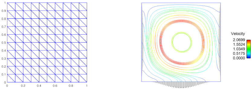
Example 1.

(Square in 2D). Let $\mathsf{\Omega }={(0,1)}^2$. To construct the triangulation ${\mathcal{T}}_h$ we first cut $\mathsf{\Omega }$ into small squares and then each square into two triangles, see Figure 1(left). The decomposition of $\partial \mathsf{\Omega }$ is defined as follows: $\mathsf{\Gamma }=(0,1)\times \left\{1\right\}$, ${\mathsf{\Gamma }}_N={\gamma }_{\mathit{left}}\cup {\gamma }_{\mathit{right}}$, $S=(0,1)\times \left\{0\right\}$, where ${\gamma }_{\mathit{left}}=\left\{0\right\}\times (0,1)$, ${\gamma }_{\mathit{right}}=\left\{1\right\}\times (0,1)$. Further $f=-2\mu div𝔻\left(u_{\mathit{exp}}\right)+\nabla p_{\mathit{exp}}$ in $\mathsf{\Omega }$, $\mu =1/2$, $u=0$ on $\mathsf{\Gamma }$, ${\sigma }_N=2\mu 𝔻\left(u_{\mathit{exp}}\right)n-p_{\mathit{exp}}n$ on ${\mathsf{\Gamma }}_N$, $g=15$, and $\kappa =30$ on S (see Remark 5), where $u_{\mathit{exp}}=(u_{\mathit{exp},1},u_{\mathit{exp},2})$, and

$$\begin{array}{ccc}\hfill u_{\mathit{exp},1}(x,y)& =& (1-cos(2\pi x\left)\right)sin\left(2\pi y\right),\hfill \\ \hfill u_{\mathit{exp},2}(x,y)& =& sin\left(2\pi x\right)(cos(2\pi y)-1),\hfill \\ \hfill p_{\mathit{exp}}(x,y)& =& 2\pi (-cos(2\pi x)+2cos(2\pi y)+1).\hfill \end{array}$$

Figure 1. Two-dimensional (2D) mesh (left) and streamlines (right); $g=15$, $\kappa =30$.

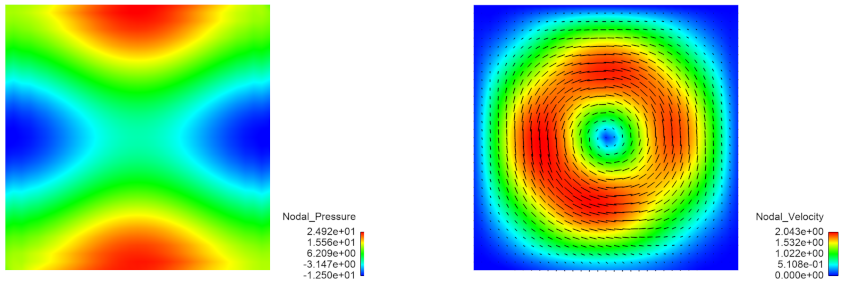
Note that $u_{\mathit{exp}}$ satisfies the homogeneous Dirichlet boundary condition on $\partial \mathsf{\Omega }$. Data are chosen in such a way that both, leak and no leak zones appear on S. Figure 1 (right) presents the streamlines of the computed solution. One can see that the leak on S generates the fluid suction on ${\mathsf{\Gamma }}_N$. Figure 2 shows the pressure and velocity distribution in $\mathsf{\Omega }$. 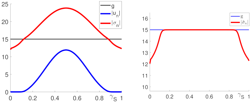The magnitudes of the normal velocity $|u_n|$ and of the normal stress $|{\sigma }_n|$ on S are seen in Figure 3 (left), while $|{\tilde{\sigma }}_n|$ is depicted in Figure 3 (right). In the tables below the values $n_{\mathit{it}}$, $n_{\mathit{F}}$, and CPU time (in seconds) for different finite element meshes with increasing $n_u$, $n_p$, and $n_s$, and different values of g are compared. The computational complexities for $g=15$ are shown in Table 1. The analogous characteristics for $g=0.1$ (leak everywhere) and $g=100$ (no leak) are summarized in Table 2 and Table 3, respectively. In view of the values of $n_{\mathit{F}}$, one can see that both algorithms are scalable. The computations without preconditioning are considerably less efficient as it is seen from Table 4.

Figure 2. The pressure (left) and velocity (right) distribution; $g=15$, $\kappa =30$.

Figure 3. Distribution of $|u_n|$, $|{\sigma }_n|$ (left) and $|{\tilde{\sigma }}_n|$ (right) on S; $g=15$, $\kappa =30$.

Table 1. Computations with preconditioner for $g=15$, $\kappa =30$.

	Algorithm PF		Algorithm SSN
${\mathit{n}}_{\mathit{u}}/{\mathit{n}}_{\mathit{p}}/{\mathit{n}}_{\mathit{s}}$	time(s.)	${\mathit{n}}_{\mathit{it}}/{\mathit{n}}_{\mathit{F}}$	time(s.)	${\mathit{n}}_{\mathit{it}}/{\mathit{n}}_{\mathit{F}}$
8320/4225/65	1.2	12/171	0.7	6/97
18,624/9409/97	3.7	12/194	2.8	8/139
33,024/16,641/129	8.4	12/209	4.8	7/129
51,520/25,921/161	15.5	12/231	10.2	8/150
74,112/37,249/193	23.8	12/228	15.7	7/139
100,800/50,625/225	42.4	12/260	25.5	7/147
131,584/66,049/257	62.4	12/266	38.5	7/147
166,464/83,521/289	82.9	12/251	58.3	7/156
205,440/103,041/321	118.0	12/261	78.3	7/153
248,512/124,609/353	172.0	13/295	110.0	7/164

Table 2. Computations with preconditioner for $g=0.1$, $\kappa =30$.

	Algorithm PF		Algorithm SSN
${\mathit{n}}_{\mathit{u}}/{\mathit{n}}_{\mathit{p}}/{\mathit{n}}_{\mathit{s}}$	time(s.)	${\mathit{n}}_{\mathit{it}}/{\mathit{n}}_{\mathit{F}}$	time(s.)	${\mathit{n}}_{\mathit{it}}/{\mathit{n}}_{\mathit{F}}$
8320/4225/65	1.1	10/131	0.8	6/88
18,624/9409/97	3.0	11/144	2.3	6/97
33,024/16,641/129	6.4	12/178	3.7	6/100
51,520/25,921/161	12.0	12/181	8.3	7/120
74,112/37,249/193	16.6	10/164	16.1	7/131
100,800/50,625/225	32.0	12/190	18.5	5/89
131,584/66,049/257	48.7	12/196	35.3	7/137
166,464/83,521/289	76.1	13/221	50.4	7/134
205,440/103,041/321	110.5	14/237	72.5	7/142
248,512/124,609/353	128.0	12/211	99.8	7/147

Table 3. Computations with preconditioner for $g=100$, $\kappa =30$.

	Algorithm PF		Algorithm SSN
${\mathit{n}}_{\mathit{u}}/{\mathit{n}}_{\mathit{p}}/{\mathit{n}}_{\mathit{s}}$	time(s.)	${\mathit{n}}_{\mathit{it}}/{\mathit{n}}_{\mathit{F}}$	time(s.)	${\mathit{n}}_{\mathit{it}}/{\mathit{n}}_{\mathit{F}}$
8320/4225/65	1.2	9/150	0.8	6/87
18,624/9409/97	3.9	9/190	2.1	7/116
33,024/16,641/129	12.6	11/294	6.6	8/142
51,520/25,921/161	15.4	11/275	8.1	6/102
74,112/37,249/193	28.2	10/244	20.2	9/172
100,800/50,625/225	42.7	10/251	24.5	7/134
131,584/66,049/257	61.4	10/258	26.2	5/88
166,464/83,521/289	86.8	10/263	54.7	7/143
205,440/103,041/321	121.6	10/271	85.3	8/168
248,512/124,609/353	164.8	10/281	95.1	7/139

Table 4. Computations without preconditioner for $g=15$, $\kappa =30$.

	Algorithm PF		Algorithm SSN
${\mathit{n}}_{\mathit{u}}/{\mathit{n}}_{\mathit{p}}/{\mathit{n}}_{\mathit{s}}$	time(s.)	${\mathit{n}}_{\mathit{it}}/{\mathit{n}}_{\mathit{F}}$	time(s.)	${\mathit{n}}_{\mathit{it}}/{\mathit{n}}_{\mathit{F}}$
8320/4225/65	13.0	27/1554	9.1	13/1450
18,624/9409/97	36.3	31/1865	30.8	20/2036
33,024/16,641/129	103.0	33/2484	82.0	20/2352
51,520/25,921/161	239.6	39/3371	188.5	15/3164
74,112/37,249/193	459.8	42/4089	343.6	14/3672

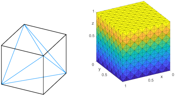
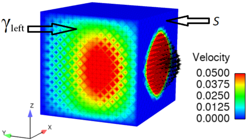
Example 2.

(Cube in 3D). Let $\mathsf{\Omega }={(0,1)}^3$. To construct the partition ${\mathcal{T}}_h$ we first cut $\mathsf{\Omega }$ into small cubes and then each cube is split into five tetrahedras, see Figure 4. The partition of $\partial \mathsf{\Omega }$ into $\mathsf{\Gamma }$, S, and ${\mathsf{\Gamma }}_N$ is defined as follows: $\mathsf{\Gamma }={\gamma }_{\mathit{top}}\cup {\gamma }_{\mathit{bottom}}\cup {\gamma }_{\mathit{back}}$, ${\mathsf{\Gamma }}_N={\gamma }_{\mathit{left}}\cup {\gamma }_{\mathit{right}}$, $S={\gamma }_{\mathit{front}}$, where ${\gamma }_{\mathit{bottom}}=(0,1)\times (0,1)\times \left\{0\right\}$, ${\gamma }_{\mathit{top}}=(0,1)\times (0,1)\times \left\{1\right\}$, ${\gamma }_{\mathit{back}}=\left\{1\right\}\times (0,1)\times (0,1)$, ${\gamma }_{\mathit{left}}=(0,1)\times \left\{0\right\}\times (0,1)$, ${\gamma }_{\mathit{right}}=(0,1)\times \left\{1\right\}\times (0,1)$, ${\gamma }_{\mathit{front}}=\left\{0\right\}\times (0,1)\times (0,1)$. Further $f=-2\mu div𝔻\left(u_{\mathit{exp}}\right)+\nabla p_{\mathit{exp}}$ in $\mathsf{\Omega }$, $\mu =1/2$, $u=0$ on $\mathsf{\Gamma }$, ${\sigma }_N=2\mu 𝔻\left(u_{\mathit{exp}}\right)n-p_{\mathit{exp}}n$ on ${\mathsf{\Gamma }}_N$, $g=15$, and $\kappa =30$, where $u_{\mathit{exp}}=(u_{\mathit{exp},1},u_{\mathit{exp},2},u_{\mathit{exp},3})$, and

$$\begin{array}{ccc}\hfill u_{\mathit{exp},1}(x,y,z)& =& 4(1-cos(2\pi x\left)\right)sin\left(2\pi y\right)z(1-z),\hfill \\ \hfill u_{\mathit{exp},2}(x,y,z)& =& 4sin\left(2\pi x\right)(cos(2\pi y)-1)z(1-z),\hfill \\ \hfill u_{\mathit{exp},3}(x,y,z)& =& 0,\hfill \\ \hfill p_{\mathit{exp}}(x,y,z)& =& 2\pi (-cos(2\pi x)+2cos(2\pi y)-cos(2\pi z\left)\right).\hfill \end{array}$$

Figure 4. Splitting of the small cube (left) and 3D mesh (right); 1728 cubes and 8640 tetrahedras.

Again, $u_{\mathit{exp}}$ satisfies the homogeneous Dirichlet boundary condition on $\partial \mathsf{\Omega }$ and data are chosen in such a way that both, leak and no leak zones appear on S. Figure 5 shows the distribution of the velocity field on S and ${\mathsf{\Gamma }}_N$. One can see the leak zone in the middle of S and the fluid suction on ${\gamma }_{\mathit{left}}$. The same suction effect appears on ${\gamma }_{\mathit{right}}$. 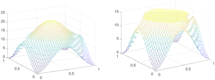The normal stress $|{\sigma }_n|$ and $|{\tilde{\sigma }}_n|$ on S are seen in Figure 6. In Table 5, Table 6, Table 7 and Table 8 we summarize analogous characteristics as in Example 1. The conclusions are also analogous, i.e., both algorithms turn out to be scalable also in 3D and the preconditioner plays an important role. Notice that the numbers $n_F$ of the matrix-vector multiplications are lower compared to 2D case.

Figure 5. Velocity field on S and ${\mathsf{\Gamma }}_N$; $g=15$, $\kappa =30$.

Figure 6. Distribution of $|{\sigma }_n|$ (left) and $|{\tilde{\sigma }}_n|$ (right) on S; $g=15$, $\kappa =30$.

Table 5. Computations with preconditioner for $g=15$, $\kappa =30$.

	Algorithm PF		Algorithm SSN
${\mathit{n}}_{\mathit{u}}/{\mathit{n}}_{\mathit{p}}/{\mathit{n}}_{\mathit{s}}$	time(s.)	${\mathit{n}}_{\mathit{it}}/{\mathit{n}}_{\mathit{F}}$	time(s.)	${\mathit{n}}_{\mathit{it}}/{\mathit{n}}_{\mathit{F}}$
5148/2197/143	0.9	11/100	0.4	6/67
12,240/4913/255	3.2	11/107	1.3	6/66
23,940/9261/399	12.5	11/120	6.3	6/77
41,400/15,625/575	31.3	11/128	16.2	6/79
65,772/24,389/783	73.7	11/140	34.7	6/77
98,208/35,937/1023	136.8	11/137	68.5	6/77
139,860/50,653/1295	280.8	12/155	124.0	6/77
191,880/68,921/1599	502.9	12/162	235.6	6/83

Table 6. Computations with preconditioner for $g=0.1$, $\kappa =30$.

	Algorithm PF		Algorithm SSN
${\mathit{n}}_{\mathit{u}}/{\mathit{n}}_{\mathit{p}}/{\mathit{n}}_{\mathit{s}}$	time(s.)	${\mathit{n}}_{\mathit{it}}/{\mathit{n}}_{\mathit{F}}$	time(s.)	${\mathit{n}}_{\mathit{it}}/{\mathit{n}}_{\mathit{F}}$
5148/2197/143	0.8	11/87	0.4	6/66
12,240/4913/255	3.9	13/95	1.7	7/76
23,940/9261/399	9.8	11/90	5.7	6/72
41,400/15,625/575	26.5	13/101	12.9	6/64
65,772/24,389/783	55.7	11/101	23.9	5/54
98,208/35,937/1023	137.0	15/127	45.8	5/54
139,860/50,653/1295	246.1	14/126	82.7	5/55
191,880/68,921/1599	400.6	13/119	145.5	5/56

Table 7. Computations with preconditioner for $g=100$, $\kappa =30$.

	Algorithm PF		Algorithm SSN
${\mathit{n}}_{\mathit{u}}/{\mathit{n}}_{\mathit{p}}/{\mathit{n}}_{\mathit{s}}$	time(s.)	${\mathit{n}}_{\mathit{it}}/{\mathit{n}}_{\mathit{F}}$	time(s.)	${\mathit{n}}_{\mathit{it}}/{\mathit{n}}_{\mathit{F}}$
5148/2197/143	1.0	8/92	0.4	6/71
12,240/4913/255	3.7	8/99	2	7/77
23,940/9261/399	12.5	8/134	6.2	6/76
41,400/15,625/575	33.6	8/138	16.1	6/77
65,772/24,389/783	57.7	7/116	34.5	6/76
98,208/35,937/1023	139.0	8/141	68.7	6/77
139,860/50,653/1295	249.7	8/145	140	7/92
191,880/68,921/1599	400.7	8/133	166.9	4/64

Table 8. Computations without preconditioner for $g=15$, $\kappa =30$.

	Algorithm PF		Algorithm SSN
${\mathit{n}}_{\mathit{u}}/{\mathit{n}}_{\mathit{p}}/{\mathit{n}}_{\mathit{s}}$	time(s.)	${\mathit{n}}_{\mathit{it}}/{\mathit{n}}_{\mathit{F}}$	time(s.)	${\mathit{n}}_{\mathit{it}}/{\mathit{n}}_{\mathit{F}}$
5148/2197/ 143	21.7	41/2963	14.0	9/1940
12,240/4913/255	86.5	32/2700	40.6	9/2198
23,940/9261/399	688.7	59/7857	273.7	10/3281
41,400/15,625/575	1549.6	46/6909	796.5	10/3673

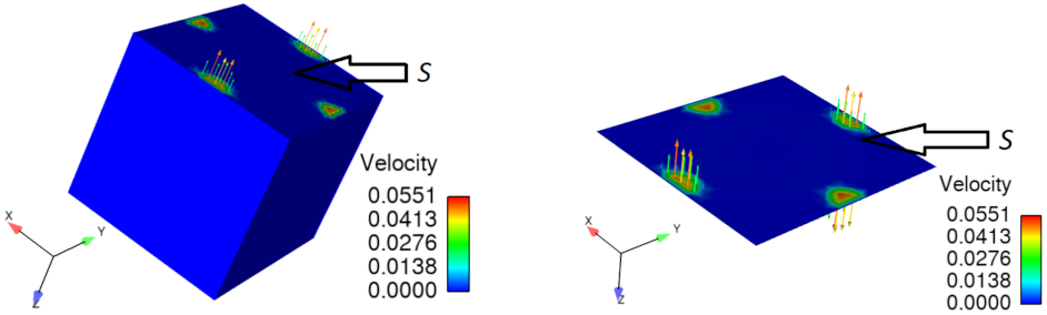
Example 3.

(Cube in 3D, non-unique solution). We change the partition of $\partial \mathsf{\Omega }$ from Example 2 as follows: ${\mathsf{\Gamma }}_N=\varnothing$, $\mathsf{\Gamma }={\gamma }_{\mathit{left}}\cup {\gamma }_{\mathit{right}}\cup {\gamma }_{\mathit{back}}\cup {\gamma }_{\mathit{front}}\cup {\gamma }_{\mathit{top}}$, and $S={\gamma }_{\mathit{bottom}}$. Let us remind that, if ${\mathsf{\Gamma }}_N=\varnothing$, the pressure might be non-unique depending on the choice of g. Next we suppose that g is constant and $\kappa =0$ on S. To establish the critical value of g we use the Stokes system with the homogeneous Dirichlet data prescribed on the whole boundary $\partial \mathsf{\Omega }$. Assuming that its solution is smooth enough, $g_{\mathit{crit}}=({sup}_S\left({\sigma }_n\right)-{inf}_S\left({\sigma }_n\right))/2$, where ${\sigma }_n$ is the corresponding normal stress. However since the whole procedure is applied to the finite element discretization, the regularity assumption is superfluous. For given physical data and the partition ${\mathcal{T}}_h$ characterized by the parameters $n_u/n_p/n_s=38,088/15,625/529$ the value $g_{\mathit{crit}}=18.31$. It is easy to show that if $g<g_{\mathit{crit}}$, the problem has a unique solution with both, leak and no-leak zones on S. If $g>g_{\mathit{crit}}$, the solution is not unique and only no-leak zone appears on S. The behavior of the algorithms for different g is summarized in Table 9. One can see that both algorithms are stable in all cases. The table presents also the values ${sup}_S\left({\sigma }_n^g\right)$ and ${inf}_S\left({\sigma }_n^g\right)$ computed for the respective g. One can easily check that $({sup}_S\left({\sigma }_n^g\right)-{inf}_S\left({\sigma }_n^g\right))/2=g_{\mathit{crit}}$ for $g\ge g_{\mathit{crit}}$, while $({sup}_S\left({\sigma }_n^g\right)-{inf}_S\left({\sigma }_n^g\right))/2=g$ if $g<g_{\mathit{crit}}$. The distribution of the velocity field on S for $g=16.31$ is seen from Figure 7. Note that the matrix $\mathbf{C}$ used in (25), especially its part ${({\mathbf{N}}^T,{\mathbf{B}}^T)}^T$, has not the full row-rank due to ${\mathsf{\Gamma }}_N=\varnothing$. Consequently, ${\mathbf{F}}_{\kappa }$ and ${\mathbf{F}}^{\left(k\right)}$ for ${\mathcal{A}}_0={\mathcal{N}}_0$ are singular with the defect one and the eigenvector whose all components are equal to 1 corresponds to the zero eigenvalue. The matrix ${\mathbf{S}}_{\kappa }^{\left(k\right)}$ of the inner linear systems in Algorithm PF is regularized by adding the diagonal matrix ${\mathbf{J}}_{12}{\mathbf{M}}^{\left(k\right)}{\left({\mathbf{Z}}^{\left(k\right)}\right)}^{-1}{\mathbf{J}}_{12}^T$ to ${\mathbf{F}}_{\kappa }$ as seen from (31) (there are non-zero diagonal entries on the level of $\mathbf{N}$). Analogously, the matrix ${\mathbf{S}}^{\left(k\right)}$ in Algorithm SSN is regularized by adding ${\mathbf{D}}^{\left(k\right)}$ to ${\mathbf{F}}^{\left(k\right)}$ (see (41)) and by the choice of the active set ${\mathcal{A}}_0\ne {\mathcal{N}}_0$. These heuristic arguments show that the matrices of the solved linear systems can be regularized by the construction of the algorithms. Finally note that the condition number bounds of the preconditioned Schur complements (32) and (42) are no longer valid. Nevertheless, the preconditioners can still be used and play the same important role as in the previous examples.

Table 9. Computations with different g and $\kappa =0$ for ${\mathsf{\Gamma }}_N=\varnothing$ ($n_u/n_p/n_s=38,088/15,625/529$).

	Algorithm PF		Algorithm SSN
$\mathit{g}$	${\mathbf{inf}}_{\mathit{S}}\left({\mathit{\sigma }}_{\mathit{n}}^{\mathit{g}}\right)/{\mathbf{sup}}_{\mathit{S}}\left({\mathit{\sigma }}_{\mathit{n}}^{\mathit{g}}\right)$	time(s.)	${\mathit{n}}_{\mathit{it}}/{\mathit{n}}_{\mathit{F}}$	time(s.)	${\mathit{n}}_{\mathit{it}}/{\mathit{n}}_{\mathit{F}}$
$g_{\mathit{crit}}+2$	$-19.86/16.76$	106.1	18/615	32.3	7/192
$g_{\mathit{crit}}+0.5$	$-18.60/18.02$	104.9	20/581	39.7	8/232
$g_{\mathit{crit}}+0.2$	$-18.40/18.22$	113.9	21/662	39.1	8/234
$g_{\mathit{crit}}$	$-18.31/18.31$	118.7	21/682	38.5	8/231
$g_{\mathit{crit}}-0.2$	$-18.11/18.11$	105.8	21/619	40.3	8/234
$g_{\mathit{crit}}-0.5$	$-17.81/17.81$	83.5	18/462	34.3	8/201
$g_{\mathit{crit}}-2$	$-16.31/16.31$	53.9	15/189	24.4	7/156

Figure 7. Distribution of the velocity field on S for $g=16.31$, $\kappa =0$, and ${\mathsf{\Gamma }}_N=\varnothing$; the whole cube (left) and S (right).

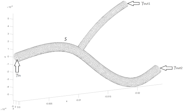
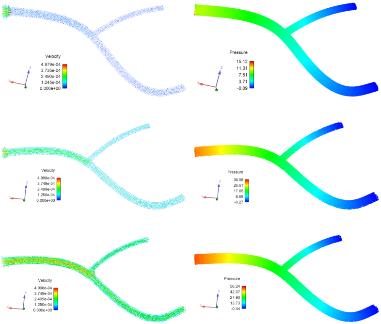
Example 4.

(3D branched tube). Let $\mathsf{\Omega }$ be the branched tube as in Figure 8, where the partition ${\mathcal{T}}_h$ and the partition of the boundary $\partial \mathsf{\Omega }=\overline{S}\cup \overline{{\gamma }_{\mathit{in}}}\cup \overline{{\gamma }_{\mathit{out}\mathit{1}}}\cup \overline{{\gamma }_{\mathit{out}\mathit{2}}}$ is also depicted. This tube may represent a final part of the capillary in the human body. On $\mathsf{\Gamma }={\gamma }_{\mathit{in}}$ we prescribe the input velocity $u_{|\mathsf{\Gamma },1}=a-a/r^2(y^2+z^2)$, $u_{|\mathsf{\Gamma },2}=u_{|\mathsf{\Gamma },3}=0$ with $a=5·{10}^{-4}$, $r=5.94·{10}^{-4}$ while ${\mathsf{\Gamma }}_N={\gamma }_{\mathit{out}\mathit{1}}\cup {\gamma }_{\mathit{out}\mathit{2}}$ consists of two outputs of the tube with the natural outflow condition ${\sigma }_N=0$. The leak condition is prescribed on $S=\partial \mathsf{\Omega }\setminus \overline{\mathsf{\Gamma }\cup {\mathsf{\Gamma }}_N}$. Further $f=0$ in $\mathsf{\Omega }$, $\mu =1/2$, and $\kappa =30$. The partition ${\mathcal{T}}_h$ is characterized by the following values of the parameters: $n_u=27,408$, $n_p=9178$, and $n_s=4079$. The behavior of Algorithm PF and Algorithm SSN for different g is reported in Table 10. The distribution of the velocity and the pressure for three selected g is depicted in Figure 9. Almost all liquid leak through the wall at the vicinity of ${\gamma }_{\mathit{in}}$ for the smallest value $g=10$ can be observed, see Figure 9 (top). The leak through the wall is minimal for $g=50$, see Figure 9 (bottom). 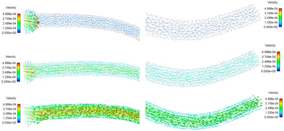The pressure is also growing for higher values of g. The zoomed parts of the velocity fields near ${\gamma }_{\mathit{in}}$ and ${\gamma }_{\mathit{out}\mathit{2}}$ are depicted in Figure 10 (the velocity distribution inside the tube looks like the Poiseuille distribution). We used the reorthogonalization technique of the descent vectors inside the CGM solver [44] that increases considerably efficiency of computations; compare Table 10 with Table 11.

Figure 8. Branched tube: mesh.

Table 10. Computations for different values of g with reorthogonalization.

	Algorithm PF		Algorithm SSN
$\mathit{g}$	time(s.)	${\mathit{n}}_{\mathit{it}}/{\mathit{n}}_{\mathit{F}}$	time(s.)	${\mathit{n}}_{\mathit{it}}/{\mathit{n}}_{\mathit{F}}$
10	3018	26/3511	1369	15/1882
20	3122	26/3805	1348	15/1885
30	3146	25/3934	1370	15/1882
40	3622	26/4291	1096	13/1522
50	3948	26/4508	995	12/1377

Figure 9. Distribution of the velocity (left) and the pressure (right) for $g=10,30,50$.

Figure 10. Distribution of the velocity near ${\gamma }_{in}$ (left) and ${\gamma }_{\mathit{out}\mathit{2}}$ (right) for $g=10,30,50$.

Table 11. Computations for different values of g without reorthogonalization.

	Algorithm PF		Algorithm SSN
$\mathit{g}$	time(s.)	${\mathit{n}}_{\mathit{it}}/{\mathit{n}}_{\mathit{F}}$	time(s.)	${\mathit{n}}_{\mathit{it}}/{\mathit{n}}_{\mathit{F}}$
10	8314	25/11,017	15,584	15/21,214
20	9927	25/12,594	14,934	14/21,344
30	10,866	25/13,861	11,156	14/16,653
40	10,815	26/15,520	11,696	12/16,473
50	12,801	26/16,622	18,673	9/24,300

6. Conclusions and Comments

We have proposed two algorithms for solving the Stokes flow with the threshold leak boundary condition, both based on dual strategies. Unlike the threshold slip boundary conditions [28], the algorithms are identical in 2D and 3D. Algorithm PF is based on the path-following variant of the interior point method that generates strictly feasible iterations. This algorithm combines the dumped Newton method in the outer loop with the preconditioned conjugate gradient method used for solving the inner linear systems. The precision control of the inner loop is driven adaptively with respect to the accuracy achieved in the outer level. The crucial ingredient of the algorithm is its diagonal preconditioner that improves ill-conditioning of the system matrices in the later iterations of the outer loop. Algorithm SSN uses the active-set implementation of the semi-smooth Newton method adapted for our type of boundary conditions. The inner linear systems are solved using the same ideas as in Algorithm PF. In this case, the diagonal preconditioner improves ill-conditioning caused by small finite element mesh norms. Experimental scalability of both algorithms is indicated by numerical experiments. Indeed, one can conclude that Algorithm SSN is more efficient than Algorithm PF. Problems with multiple solutions can be also solved since the singular dual Hessian is implicitly regularized by the construction of the algorithms.