Chaos for the Dynamics of Toeplitz Operators

Abstract

Chaotic properties in the dynamics of Toeplitz operators on the Hardy–Hilbert space ${\mathcal{H}}^2\left(\mathbb{D}\right)$ are studied. Based on previous results of Shkarin and Baranov and Lishanskii, a characterization of different versions of chaos formulated in terms of the coefficients of the symbol for the tridiagonal case are obtained. In addition, easily computable sufficient conditions that depend on the coefficients are found for the chaotic behavior of certain Toeplitz operators.

1. Introduction

Hypercyclic (that is, topologically transitive) and chaotic operators on separable Banach spaces have been studied for more than twenty years (the reader is referred to the work in [1,2] for good sources on linear dynamics). On the other hand, Toeplitz operators were introduced by Otto Toeplitz in [3]. They are among the most studied families of operators on the Hardy–Hilbert space. On this space, the matrices of Toeplitz operators (with respect to the canonical basis) have constant diagonals.

A Toeplitz operator $T_{\mathrm{\Phi }}:{\mathcal{H}}^2\left(\mathbb{D}\right)\to {\mathcal{H}}^2\left(\mathbb{D}\right)$ on the Hardy–Hilbert space ${\mathcal{H}}^2\left(\mathbb{D}\right)$ with symbol $\mathrm{\Phi }\in L^{\infty }\left(\mathbb{T}\right)$ is defined by $T_{\mathrm{\Phi }}\left(f\right)=P\left(M_{\mathrm{\Phi }}\left(f\right)\right)$, $f\in {\mathcal{H}}^2\left(\mathbb{D}\right)$, where $M_{\mathrm{\Phi }}$ is the multiplication operator by $\mathrm{\Phi }$ and $P:L^2\left(\mathbb{T}\right)\to {\mathcal{H}}^2\left(\mathbb{D}\right)$ is the Riesz projection. Here, as usual, $\mathbb{D},\mathbb{T}\subset \mathbb{C}$ are the open unit disc and its boundary, the unit circle, respectively. Actually,

$${\mathcal{H}}^2\left(\mathbb{D}\right)=\{f:\mathbb{D}\to \mathbb{C};f\left(z\right)=\sum _{n\ge 0}{a}_n{z}^n\mathrm{with}\sum _{n\ge 0} |a_n{|}^2<\infty \},$$

so that it is naturally identified with the Hilbert sequence space ${\ell }^2$. The reader is referred to the work in [4] for the basic theory of Toeplitz operators, and to the work in [5,6] for a detailed study of Hardy spaces.

It is known that analytic Toeplitz operators, that is, operators whose symbol is in ${\mathcal{H}}^{\infty }$ (the space of all the functions that are analytic and bounded on the open unit disk), cannot be hypercyclic, as their adjoints always have eigenvalues. However, Toeplitz operators with anti-analytic symbols, i.e., such that the symbol $\mathrm{\Phi }$ satisfies $\mathrm{\Phi }(1/z)\in {\mathcal{H}}^{\infty }$, provide many examples of hypercyclic operators, and they are the most studied Toeplitz operators in the topic of chaotic dynamics. Godefroy and Shapiro [7] showed that a Toeplitz operator $T_{\overline{\mathrm{\Phi }}}$ with anti-analytic symbol $\overline{\mathrm{\Phi }}\left(z\right)={\sum }_{n\le 0}{a}_n{z}^n$ is chaotic if, and only if, $\mathrm{\Phi }\left(\mathbb{D}\right)\cap \mathbb{T}\ne \varnothing$ for $\mathrm{\Phi }\left(z\right)={\sum }_{n\ge 0}{a}_{-n}{z}^n$, a result that was extended by De Laubenfels and Emamirad in [8] for ${\ell }^p$, $1\le p<\infty$ and $c_0$. Notice that, with the above identification of ${\mathcal{H}}^2\left(\mathbb{D}\right)$ with ${\ell }^2$, the anti-analytic Toeplitz operator $T_{\overline{\mathrm{\Phi }}}$ with $\overline{\mathrm{\Phi }}\left(z\right)={\sum }_{n\le 0}{a}_n{z}^n$ can be formally represented by

$$T_{\overline{\mathrm{\Phi }}}=\sum _{n\ge 0}{a}_{-n}{B}^n,$$

where B is the backward shift $B(x_0,x_1,...)=(x_1,x_2,...)$, so that an anti-analytic Toeplitz operator can be viewed as an upper triangular infinite matrix with constant diagonals. With this identification, Bourdon and Shapiro [9] studied the dynamics of anti-analytic Toeplitz operators in the Bergman space, and Martínez [10] in more general sequence spaces. The first example of an anti-analytic and hypercyclic Toeplitz operator was$T_{\mathsf{\lambda }/z}$ for $\left|\mathsf{\lambda }\right|>1$ [11], which is represented by $\mathsf{\lambda }B$. A special mention should be done to the exponential of the backward shift $T=e^B$ that was shown to be hypercyclic in arbitrary “small” sequence spaces in [12,13].

Baranov and Lishanskii [14], inspired by the work of Shkarin [15], studied hypercyclicity of Toeplitz operators on ${\mathcal{H}}^2\left(\mathbb{D}\right)$ with symbols of the form $p(1/z)+\phi \left(z\right)$, where p is a polynomial and $\phi \in {\mathcal{H}}^{\infty }$. They showed necessary conditions and sufficient conditions for hypercyclicity which almost coincide in the case the degree of p is one. They characterized hypercyclicity in the tridiagonal case (i.e., when p and q have degree one) by refining a result of Shkarin [15]. Based on these results, the chaotic behavior of certain non-local operators was studied in [16]. Recently, some new classes of hypercyclic Toeplitz operators were also found in [17], as a continuation of the work in [14].

In this paper, a characterization of chaos in the tridiagonal case formulated in terms of the three symbol coefficients is obtained. Sufficient conditions for chaos in more general cases, also explicit on the symbol coefficients, are shown, and they easily provide us with examples of chaotic Toeplitz operators. The main contribution of the present work in comparison to the work in [14,15] is to offer conditions on the symbol coefficients of a Toeplitz operator for chaos, which are much easier to check than the previous ones. Moreover, the characterization of the tridiagonal case gives a full picture of the chaotic behavior in terms of the three coefficients. Finally, a rich variety of chaotic properties, in the topological and in the measure theoretical sense are provided, which must be compared with previous works on the dynamics of Toeplitz operators, dealing with hypercyclicity and/or Devaney chaos.

2. Preliminaries and Notation

Some definitions about hypercyclicity and chaos need to be recalled. From now on, unless otherwise specified, X will be assumed to be an infinite dimensional separable Banach space and $T:X\to X$ a continuous and linear operator.

An operator $T:X\to X$ is called hypercyclic if there is some $x\in X$ whose orbit under T is dense in X. In such a case, x is called a hypercyclic vector for T. The operator T is said to be Devaney chaotic if it is hypercyclic and admits a dense set of periodic points. Actually the original definition of Devaney [18] also included as an ingredient the sensitive dependence on initial conditions, but it was shown to be redundant (see, e.g., in [19]).

The first notion of chaos coined in the mathematical literature appeared in the article of Li and Yorke [20]. Let $(Y,d)$ be a metric space. A continuous map $f:Y\to Y$ is called Li–Yorke chaotic if there exists an uncountable subset $\mathrm{\Gamma }\subset Y$ such that for every pair $x,y\in \mathrm{\Gamma }$ of distinct points one has

$$\underset{n}{lim\; inf}d(f^{n}x,f^{n}y)=0\mathrm{and}\underset{n}{lim\; sup}d(f^{n}x,f^{n}y)>0.$$

In this case, $\mathrm{\Gamma }$ is a scrambled set and $\{x,y\}\subset \mathrm{\Gamma }$ a Li–Yorke pair.

A vector $x\in X$ is said to be irregular for T if ${lim\; inf}_n\parallel T^{n}x\parallel =0$ and ${lim\; sup}_n\parallel T^{n}x\parallel =\infty$.

A stronger notion of chaos was introduced by Schweizer and Smital [21]: Let $(Y,d)$ be a metric space and let $f:Y\to Y$ be a continuous map. For any pair $\{x,y\}\subset Y$ and every $n\in \mathbb{N}$, the distributional function $F_{xy}^n:{\mathbb{R}}^{+}\to [0,1]$ is defined by

$$F_{xy}{\left(\tau \right)}^n=\frac{1}{n}card\left\{0\le i\le n-1:d(f^{i}x,f^{i}y)<\tau \right\},$$

where card(A) denotes the cardinality of the set A. Define

$$F_{xy}\left(\tau \right)=\underset{n\to \infty }{lim\; inf}{F}_{xy}^n\left(\tau \right)$$

$$F_{xy}^{*}\left(\tau \right)=\underset{n\to \infty }{lim\; sup}{F}_{xy}^n\left(\tau \right)$$

The map f is called distributionally chaotic if there exist an uncountable subset $\mathrm{\Gamma }\subset Y$ and $ϵ>0$ such that for every $\tau >0$ and each pair of distinct points $x,y\in \mathrm{\Gamma }$, it happens that $F_{xy}^{*}\left(\tau \right)=1$ and $F_{xy}\left(ϵ\right)=0$. The set $\mathrm{\Gamma }$ is a distributionally $ϵ$-scrambled set and the pair $x,y$ a distributionally chaotic pair. Moreover, f exhibits dense distributional chaos if the set $\mathrm{\Gamma }$ may be chosen to be dense.

A subset A of $\mathbb{N}$ is said to have positive lower density if

$$\underline{\mathrm{dens}}\left(A\right)=\underset{N\to \infty }{lim\; inf}\frac{card\{n\le N:n\in A\}}{N}>0.$$

Inspired by Birkhoff ergodic theorem, Bayart and Grivaux [22,23] considered a concept stronger than hypercyclicity: An operator T on X is said to be frequently hypercyclic provided there exists a vector x such that for every nonempty open subset U of X, the set of integers n such that $T^{n}x$ belongs to U has positive lower density. In this case, x is called a frequently hypercyclic vector for T.

Bowen [24] introduced a very strong dynamical notion for maps on compact spaces that occurs when one can approximate distinct pieces of orbits by a single periodic orbit with a certain uniformity: A continuous map $f:K\to K$ on a compact metric space $(K,d)$ has the specification property (SP) if for any $\delta >0$ there is a positive integer $N_{\delta }$ such that for any integer $s\ge 2$, any set $\{y_1,\dots ,y_s\}\subset K$ and any integers $0=j_1\le k_1<j_2\le k_2<\cdots <j_s\le k_s$ satisfying $j_{r+1}-k_r\ge N_{\delta }$ for $r=1,\dots ,s-1$, there is a point $x\in K$ such that, for each positive integer $r\le s$ and any integer i with $j_r\le i\le k_r$, the following conditions hold:

$$d(f^i\left(x\right),f^i\left(y_r\right))<\delta ,$$

$$f^n\left(x\right)=x\mathrm{where}n=N_{\delta }+k_s.$$

Bartoll et al. [25] generalized this concept for operators: An operator T on X has the operator specification property (OSP) if there exists an increasing sequence ${\left(K_m\right)}_m$ of T-invariant sets with $0\in K_1$ and $\overline{{\cup }_{m\in \mathbb{N}}{K}_m}=X$ such that for each $m\in N$ the map $T|K_m$ has the SP.

Some measure-theoretic concepts in dynamics ought to be recalled too. Let $(X,\mathcal{B},\mu )$ be a probability space, where X is a topological space and $\mathcal{B}$ denotes the $\sigma -$ algebra of Borel subsets of X. A Borel probability measure $\mu$ is said to have full support if $\mu \left(U\right)>0$ for each non-empty open set $U\subset X$. A measurable map $T:(X,\mathcal{B},\mu )\to (X,\mathcal{B},\mu )$ is called a measure preserving transformation (or $\mu$ is T-invariant) if $\mu \left(T^{-1}\left(A\right)\right)=\mu \left(A\right)$ for all $A\in \mathcal{B}$. The measure $\mu$ is said to be strongly mixing with respect to T if

$$\underset{n\to \infty }{lim}\mu (A\cap T^{-n}\left(B\right))=\mu \left(A\right)\mu \left(B\right),\forall A,B\in \mathcal{B}.$$

A recent work that, in particular, connects the OSP with the existence of strongly mixing measures is [26].

A sufficient condition for frequent hypercyclicity was given by Bayart and Grivaux [23], later refined by Bonilla and Grosse-Erdmann [27] by replacing absolute convergence of series by unconditional convergence. This is what is known today as the Frequent Hypercyclicity Criterion. A series ${\sum }_n{x}_n$ in X converges unconditionally if it converges and, for any 0-neighborhood U in X, there exists some $N\in \mathbb{N}$ such that ${\sum }_{n\in F}{x}_n\in U$ for every finite set $F\subset \{N,N+1,N+2,\dots \}$.

It was shown in [28] that the Frequent Hypercyclicity Criterion implies the existence of mixing measures (see also in [29] for more general results).

Theorem 1

([28]). Let T be an operator on X. If there is a dense subset $X_0$ of X and a sequence of maps $S_n:X_0\to X$ such that for each $x\in X_0$.

(i) 

${\sum }_{n=0}^{\infty }{T}^{n}x$converges unconditionally,

(ii) 

${\sum }_{n=0}^{\infty }{S}_{n}x$converges unconditionally, and

(iii) 

$T^n{S}_{n}x=x$and$T^m{S}_{n}x=S_{n-m}x$if$n>m$,

then there is a $T-$invariant strongly mixing Borel probability measure μ on X with full support.

A powerful tool in linear dynamics to obtain chaotic properties for operators is to have a wide source of eigenvectors associated to suitable eigenvalues. Certainly, the basis is found in the so-called Godefroy–Shapiro Criterion [7]. Other sufficient conditions for hypercyclicity can be found in [1,2,30,31].

Theorem 2

(Godefroy–Shapiro Criterion). Let T be an operator on X. Suppose that the subspaces

$$\hspace{1em}\hspace{1em}\hspace{1em}\hspace{1em}\hspace{1em}{X}_0:=span\{x\in X:Tx=\mathsf{\lambda }x\mathit{for}\mathit{some}\mathsf{\lambda }\in \mathbb{C}\mathit{with}|\mathsf{\lambda }|<1\}$$

and

$$\hspace{1em}\hspace{1em}\hspace{1em}\hspace{1em}\hspace{1em}{Y}_0:=span\{x\in X:Tx=\mathsf{\lambda }x\mathit{for}\mathit{some}\mathsf{\lambda }\in \mathbb{C}\mathit{with}|\mathsf{\lambda }|>1\}$$

are dense in X. Then, T is hypercyclic. If, moreover, the subspace

$$Z_0:=span\{x\in X;Tx=e^{\alpha \pi i}x\mathit{for}\mathit{some}\alpha \in \mathbb{Q}\}$$

is dense in X, then T is Devaney chaotic.

Suitable eigenvector fields will be very useful to obtain all the chaotic properties considered here, an idea that follows the work initiated by Bayart and Grivaux [22]. Given an operator $T:X\to X$ on a complex Banach space X, a collection of functions $E_j:\mathbb{T}\to X$, $j\in J$, is called a spanning eigenvector field associated to unimodular eigenvalues if $E_j\left(\mathsf{\lambda }\right)\in ker(\mathsf{\lambda }I-T)$ for any $\mathsf{\lambda }\in \mathbb{T}$, $j\in J$, and

$$span\{E_j\left(\mathsf{\lambda }\right);\mathsf{\lambda }\in \mathbb{T},j\in J\}\mathrm{is}\mathrm{dense}\mathrm{in}X.$$

A map $G:U\to X$ defined on a non-empty open set $U\subset \mathbb{C}$ is said to be weakly holomorphic on U if $y\circ G:U\to \mathbb{C}$ is holomorphic for any $y\in X^{*}$.

The following result is essentially well known, but its proof is included for the sake of completeness.

Theorem 3. (Eigenfield Criterion) Given an operator

$T:X\to X$ on a complex Banach space X, if $U\subset \mathbb{C}$ is a connected nonempty open set that intersects $\mathbb{T}$, $G_j:U\to X$, $j\in J$, is a collection of weakly holomorphic maps such that $G_j\left(\mathsf{\lambda }\right)\in ker(\mathsf{\lambda }I-T)$ for any $\mathsf{\lambda }\in U$, $j\in J$, and

$$span\{G_j\left(\mathsf{\lambda }\right);\mathsf{\lambda }\in U,j\in J\}\mathit{is}\mathit{dense}\mathit{in}X,$$

then

(i) 

T is Devaney chaotic,

(ii) 

there exists a $C^{\infty }$ spanning eigenvector field associated to unimodular eigenvalues $E_j:\mathbb{T}\to X$, $j\in J$, such that $E_j\left(\mathsf{\lambda }\right)=G_j\left(\mathsf{\lambda }\right)$ for any $\mathsf{\lambda }\in I$, $j\in J$, where $I\subset \mathbb{T}$ is a non-trivial arc, and

(iii) 

T satisfies the Frequent Hypercyclicity Criterion.

Proof. 

To prove (i), consider $Y_1:=U\cap (\mathbb{C}\backslash \overline{\mathbb{D}})$, $Y_2:=U\cap \mathbb{D}$, and

$$Y_3:=U\cap \{e^{\alpha \pi i};\alpha \in \mathbb{Q}\}.$$

It will suffice to show that, given $k\in \{1,2,3\}$, and for any $y\in X^{*}$, the equality $⟨x,y⟩=0$ for every $x\in Y_k$ implies $y=0$. Actually, as the holomorphic maps $y\circ G_j$ annihilate on $Y_k$ for $k\in \{1,2,3\}$, which are sets with accumulating points in U, and U is connected, then $y\circ G_j\equiv 0$ for every $j\in J$. The assumptions imply that $y=0$, and (i) is shown.

For (ii), let $I_0\subset U\cap \mathbb{T}$ be an open arc, and let $I\subset I_0$ be a non-trivial closed sub-arc. It is possible to extend $G_j$ from I to $\mathbb{T}$ as a $C^{\infty }$ function $E_j$ such that $E_j\left(\mathsf{\lambda }\right)=0$ for all $\mathsf{\lambda }\notin I_0$ for each $j\in J$. $Ej$, $j\in J$, is a spanning eigenvector field associated to unimodular eigenvalues as

$$span\{E_j\left(\mathsf{\lambda }\right);\mathsf{\lambda }\in I,j\in J\}=span\{G_j\left(\mathsf{\lambda }\right);\mathsf{\lambda }\in I,j\in J\},$$

which is dense in X because I has accumulating points in U.

The fact that T satisfies the Frequent Hypercyclicity Criterion is a consequence of, e.g., Remark 9.10 and Theorem 9.22 in [2]. □

3. Tridiagonal Toeplitz Operators

The main purpose in this section is to reformulate the characterization of hypercyclic tridiagonal operators given by Shkarin [15] and Baranov and Lishanskii [14] to offer conditions expressed in terms of the three coefficients of the symbol.

More precisely, equivalent and sufficient conditions, expressed on the coefficients of the symbol, are provided in order to guarantee that a tridiagonal Toeplitz operator has a chaotic behavior. Tridiagonal Toeplitz operators were studied in [32] (see also in [33]) as generators of chaotic semigroups associated to birth-and-death processes.

Let $T_{\mathrm{\Phi }}:{\mathcal{H}}^2\left(\mathbb{D}\right)\to {\mathcal{H}}^2\left(\mathbb{D}\right)$ be an operator with symbol $\mathrm{\Phi }\left(z\right)=a_{1}z+a_0+\frac{a_{-1}}{z}$, where $a_{-1},a_0,a_1\in \mathbb{C}$. If $a_1$ is zero then $T_{\mathrm{\Phi }}$ is an anti-analytic operator, and there are conditions for these operators to be hypercyclic [2]. If $a_{-1}$ is zero then $T_{\mathrm{\Phi }}$ is a analytic operator, and these operators are not hypercyclic, as was mentioned before. The goal of this section is to have conditions such that these operators are chaotic when $a_1$ and $a_{-1}$ are not zero.

The previous eigenvalue criteria will be a key tool. To do this, one has to solve the equation $Tf=\mathsf{\lambda }f$. It is known that, for $f\in {\mathcal{H}}^2\left(\mathbb{D}\right)$, $T_{z}f\left(z\right)=zf\left(z\right)$ and $T_{\frac{1}{z}}f\left(z\right)=\frac{1}{z}(f\left(z\right)-f\left(0\right))$. Then $T=a_{-1}{T}_{\frac{1}{z}}+a_{0}I+a_1{T}_z$, which implies that $Tf=\mathsf{\lambda }f$ is equivalent to

$$a_{-1}\frac{f\left(z\right)-f\left(0\right)}{z}+a_{0}f\left(z\right)+a_{1}zf\left(z\right)=\mathsf{\lambda }f\left(z\right).$$

Therefore,

$$f\left(z\right)=\frac{a_{-1}f\left(0\right)}{a_1{z}^2+(a_0-\mathsf{\lambda })z+a_{-1}}.$$

If $f\left(0\right)=0$ one would have that

$$\begin{array}{ccc}\hfill (a_{-1}+(a_0-\mathsf{\lambda })z+a_1{z}^2)f\left(z\right)& =& 0,\hfill \end{array}$$

as f is an analytic function on $\mathbb{D}$ this would imply that $f\left(z\right)$ is identically zero. Therefore, $f\left(0\right)\ne 0$ and without loss of generality it is assumed that $f\left(0\right)=1$.

As it is wanted that

$$f\left(z\right)=\frac{a_{-1}}{a_1{z}^2+(a_0-\mathsf{\lambda })z+a_{-1}}$$

belongs to ${\mathcal{H}}^2\left(\mathbb{D}\right)$, then the polynomial $q_{\mathsf{\lambda }}\left(z\right):=a_1{z}^2+(a_0-\mathsf{\lambda })z+a_{-1}$ needs to have roots $z_1$ and $z_2$ with $|z_1|>1$ and $|z_2|>1$. This is equivalent to the roots of the polynomial

$$p_{\mathsf{\lambda }}\left(z\right):=z^2{q}_{\mathsf{\lambda }}(1/z)=a_{-1}{z}^2+(a_0-\mathsf{\lambda })z+a_1$$

being in $\mathbb{D}$.

To find conditions on the coefficients such that both roots of $p_{\mathsf{\lambda }}$ are in $\mathbb{D}$, the following test (see, e.g., in [34] for a proof of it) will play a key role.

Jury test: Consider the family of quadratic equations for $z\in \mathbb{C}$

$$z^2+wz+r=0,$$

where $w\in \mathbb{C}$ and $r\in \mathbb{R}$ are parameters. For a fixed r, let $E_r$ denote the set of all complex w such that the absolute value of each root is less then 1. If $\left|r\right|<1$, then

$$E_r=\left\{w\in \mathbb{C}:{\left(\frac{Re\left(w\right)}{1+r}\right)}^2+{\left(\frac{Im\left(w\right)}{1-r}\right)}^2<1\right\}.$$

Actually, dealing with the case when $a_1,a_{-1}\in \mathbb{C}$ demands to generalize the Jury test.

Lemma 1. (Generalized Jury Test).

The roots of $z^2+wz+r{e}^{i\theta }=0$, with parameters $w\in \mathbb{C}$, $\theta \in [0,2\pi [$ and $r\ge 0$, belong to $\mathbb{D}$ if and only if $r<1$ and

$$\frac{{Re(w{e}^{-i\frac{\theta }{2}})}^2}{{(1+r)}^2}+\frac{{Im(w{e}^{-i\frac{\theta }{2}})}^2}{{(1-r)}^2}<1.$$

Proof. 

By applying the Jury test to $p(z)=z^2+(w{e}^{-i\frac{\theta }{2}})z+r$, and taking into account that $p(z)=0$ if and only if $q(z{e}^{i\frac{\theta }{2}})=0$ for $q(z)=z^2+wz+r{e}^{i\theta }$, the result is obtained. □

The Generalized Jury test will be applied to the polynomial

$$\frac{1}{a_{-1}}{p}_{\mathsf{\lambda }}(z)=z^2+\frac{(a_0-\mathsf{\lambda })}{a_{-1}}z+\frac{a_1}{a_{-1}}.$$

Observe that, if its roots belong to $\mathbb{D}$, then $\frac{|a_1|}{|a_{-1}|}<1$. Therefore, from now on it is assumed that $|a_{-1}|>|a_1|>0$.

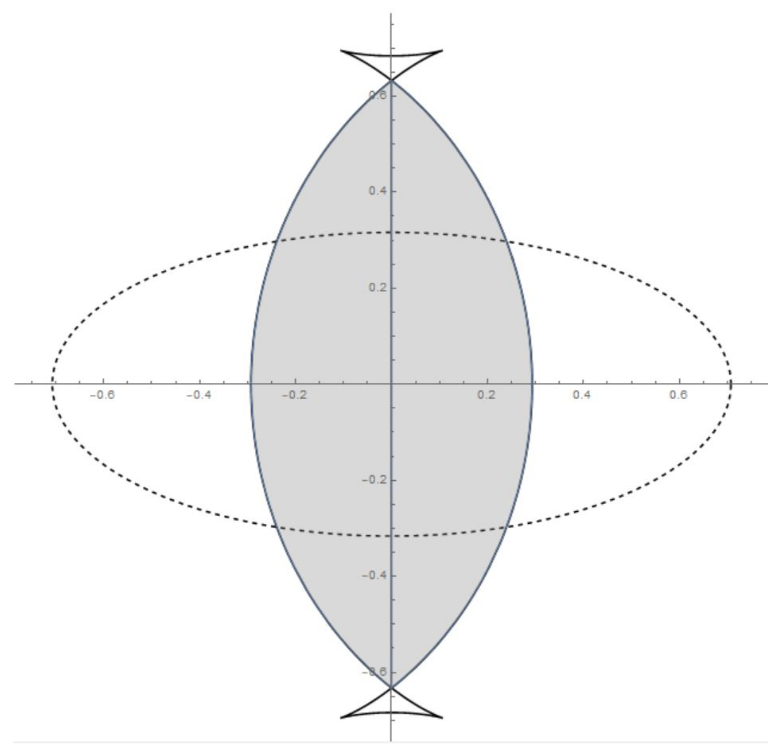
Now, consider the following ellipse:

$$E:=\left\{z\in \mathbb{C}:\frac{Re{\left(z\right)}^2}{\left(\right|a_{-1}|+|a_1{\left|\right)}^2}+\frac{Im{\left(z\right)}^2}{\left(\right|a_{-1}|-|a_1{\left|\right)}^2}=1\right\},$$

and its interior

$$E_0:=\left\{z\in \mathbb{C}:\frac{Re{\left(z\right)}^2}{\left(\right|a_{-1}|+|a_1{\left|\right)}^2}+\frac{Im{\left(z\right)}^2}{\left(\right|a_{-1}|-|a_1{\left|\right)}^2}<1\right\}.$$

Let

$$A_0:=\{z\in \mathbb{C}:d(z,E_0)<1\},$$

i.e., the interior of the outer parallel curve at distance one of the ellipse E. If $|a_{-1}|+|a_1|<1$, let F be the inner parallel curve at distance one of E. There is a connected component in the interior of F that contains 0, and its closure is set as $A_0^{\prime }$. Figure 1 illustrates an example of how $A_0^{\prime }$ is defined.

Figure 1. The dashed curve is an ellipse with major semiaxis strictly less than 1, the continuous curve is its inner parallel at distance 1, and the gray region is $A_0^{\prime }$.

All the conditions are now set to establish a key result that will allow us to obtain the desired characterization in terms of $a_0,a_1$ and $a_{-1}$.

Lemma 2.

Let $a_1,a_{-1}\in \mathbb{C}$ with $|a_1|<|a_{-1}|$. Set $a_1=\left|a_1\right|e^{i{\theta }_1}$, $a_{-1}=\left|a_{-1}\right|e^{i{\theta }_{-1}}$, with ${\theta }_1,{\theta }_{-1}\in [0,2\pi )$, $\theta =\frac{{\theta }_1+{\theta }_{-1}}{2}$. Then, the following conditions are equivalent:

(A) 

There exists$\mathsf{\lambda }\in \mathbb{T}$such that$p_{\mathsf{\lambda }}\left(z\right)=a_{-1}{z}^2+(a_0-\mathsf{\lambda })z+a_1$has its roots in$\mathbb{D}$.

(B) 

$a_0$ satisfies one of the following cases:

1. 

If$|a_{-1}|+|a_1|>1$then$a_0{e}^{-i\theta }\in A_0$.

2. 

If$|a_{-1}|+|a_1|=1$then$a_0{e}^{-i\theta }\in A_0\backslash \left\{0\right\}$.

3. 

If$|a_{-1}|+|a_1|<1$then$a_0{e}^{-i\theta }\in A_0\backslash A_0^{\prime }$.

Proof. 

By applying the Generalized Jury test to the polynomial

$$\frac{1}{a_{-1}}{p}_{\mathsf{\lambda }}(z)=z^2+\frac{(a_0-\mathsf{\lambda })}{a_{-1}}z+\frac{a_1}{a_{-1}},$$

it is known that its roots belong to $\mathbb{D}$ if, and only if, the following inequality is satisfied:

$$\frac{{Re(\frac{a_0-\mathsf{\lambda }}{a_{-1}}{e}^{-i\frac{{\theta }_1-{\theta }_{-1}}{2}})}^2}{{(1+\frac{|a_1|}{|a_{-1}|})}^2}+\frac{{Im(\frac{a_0-\mathsf{\lambda }}{a_{-1}}{e}^{-i\frac{{\theta }_1-{\theta }_{-1}}{2}})}^2}{{(1-\frac{|a_1|}{|a_{-1}|})}^2}<1,$$

which is equivalent to

$$\frac{{Re(a_0{e}^{-i\theta }-\mathsf{\lambda }{e}^{-i\theta })}^2}{\left(\right|a_1|+|a_{-1}{\left|\right)}^2}+\frac{{Im(a_0{e}^{-i\theta }-\mathsf{\lambda }{e}^{-i\theta })}^2}{\left(\right|a_1|-|a_{-1}{\left|\right)}^2}<1.$$

Let $b_0=a_0{e}^{-i\theta }$. The above inequality holds for some $\mathsf{\lambda }\in \mathbb{T}$ if, and only if, one can find ${\mathsf{\lambda }}^{\prime }\in \mathbb{T}$ such that $b_0-{\mathsf{\lambda }}^{\prime }\in E_0$. This is in turn equivalent to the existence of $z_1,z_2\in E_0$ such that $|b_0-z_1|<1$ and $|b_0-z_2|>1$. Indeed, one implication is obvious since $E_0$ is open, and the other one follows from an easy connectedness argument: Consider the function $f:E_0\to \mathbb{R}$ defined by $f\left(z\right)=|b_0-z|$. As $E_0$ is a connected set, the set $f\left(E_0\right)$ is an interval in $\mathbb{R}$ that has points greater than 1, and smaller than 1, so 1 is inside.

The equivalence with condition (B) will be shown now:

1.

$|a_1|+|a_{-1}|>1$.

As in this case $b_0\in A_0$, by the definition of the set $A_0$ it is clear that exist $z_1,z_2\in E_0$ such that $|b_0-z_1|<1$ and $|b_0-z_2|>1$.

2.

$|a_1|+|a_{-1}|=1$.

As in this case $b_0\in A_0\backslash \left\{0\right\}$, the same reasoning as above holds for all $b_0\in A_0$, except for $b_0=0$.

3.

$|a_1|+|a_{-1}|<1$.

As $b_0\in A_0\backslash A_0^{\prime }$, by the definition of $A_0$, there exists $z_1\in E_0$ such that $|b_0-z_1|<1$. Now, as $b_0\notin A_0^{\prime }$, the definition of $A_0^{\prime }$ allows us to find a point $z_2\in E_0$ such that $|b_0-z_2|>1$.

□

Therefore, far it has been characterized the existence of $\mathsf{\lambda }\in \mathbb{T}$ such that the $\mathsf{\lambda }$-eigenvector of $T_{\mathrm{\Phi }}$

$$f_{\mathsf{\lambda }}\left(z\right)=\frac{a_{-1}}{a_1{z}^2+(a_0-\mathsf{\lambda })z+a_{-1}}$$

belongs to ${\mathcal{H}}^2\left(\mathbb{D}\right)$. Actually, it will be shown that this defines an eigenvector field that satisfies the conditions of Theorem 3.

Theorem 4.

Let $B\subset \mathbb{C}$ be an open subset with non empty intersection with $\mathbb{T}$ and suppose that $f_{\mathsf{\lambda }}\in {\mathcal{H}}^2\left(\mathbb{D}\right)$ for any $\mathsf{\lambda }\in B$, where

$$f_{\mathsf{\lambda }}\left(z\right):=\frac{a_{-1}}{a_1{z}^2+(a_0-\mathsf{\lambda })z+a_{-1}}.$$

Then, the map $G:B\to {\mathcal{H}}^2\left(\mathbb{D}\right)$, $G\left(\mathsf{\lambda }\right):=f_{\mathsf{\lambda }}$, is weakly holomorphic and

$$span\{G\left(\mathsf{\lambda }\right);\mathsf{\lambda }\in B\}\mathit{is}\mathit{dense}\mathit{in}{\mathcal{H}}^2\left(\mathbb{D}\right).$$

Proof. 

For $A\subset \mathbb{C}$ open, set $\mathcal{H}\left(A\right):=\{f:A\to \mathbb{C};f \mathrm{is} \mathrm{analytic}\}$. Let g be a function in ${\mathcal{H}}^2\left(\mathbb{D}\right)$. It will be shown that, if $⟨f_{\mathsf{\lambda }},g⟩=0$ for all $\mathsf{\lambda }$ in B, then $g=0$, which is equivalent to the fact that

$$Z:=span\{f_{\mathsf{\lambda }};\mathsf{\lambda }\in B\}$$

is dense in ${\mathcal{H}}^2\left(\mathbb{D}\right)$.

Consider $H:B\to \mathbb{C}$ defined by $H\left(\mathsf{\lambda }\right):=⟨f_{\mathsf{\lambda }},g⟩$, $i.e.$,

$$H\left(\mathsf{\lambda }\right)=\frac{1}{2\pi }{\int }_0^{2\pi }\frac{a_{-1}}{q_{\mathsf{\lambda }}\left(e^{i\theta }\right)}\overline{g\left(e^{i\theta }\right)}d\theta ,\mathrm{where}{q}_{\mathsf{\lambda }}\left(z\right)=a_1{z}^2+(a_0-\mathsf{\lambda })z+a_{-1}.$$

Suppose that $H\left(\mathsf{\lambda }\right)=0$ for all $\mathsf{\lambda }\in B$. Thus, all the derivatives of H vanish at certain $e^{i\alpha }\in \mathbb{T}\cap B$. That is, $H\left(e^{i\alpha }\right)=0$,

$$\frac{dH}{d\mathsf{\lambda }}\left(e^{i\alpha }\right)=\frac{1}{2\pi }{\int }_0^{2\pi }\frac{e^{i\theta }}{q_{e^{i\alpha }}\left(e^{i\theta }\right)}h\left(\theta \right)d\theta =0,\mathrm{where}h\left(\theta \right):=\frac{a_{-1}}{q_{e^{i\alpha }}\left(e^{i\theta }\right)}\overline{g\left(e^{i\theta }\right)},$$

and

$${\int }_0^{2\pi }{\mathrm{\Phi }}^n\left(\theta \right)h\left(\theta \right)d\theta =0\mathrm{for}n=0,1,2,\dots \mathrm{where}\mathrm{\Phi }\left(\theta \right):=\frac{e^{i\theta }}{q_{e^{i\alpha }}\left(e^{i\theta }\right)}.$$

One has that $\mathrm{\Psi }\left(z\right)=\frac{z}{q_{e^{i\alpha }}\left(z\right)}$ is an analytic function in an open disc $U\supset \overline{\mathbb{D}}$. As it is known that $|a_{-1}|>|a_1|$, then $\mathrm{\Psi }$ is univalent on a neighborhood of $\overline{\mathbb{D}}$, which is assumed to be U, and there exists ${\mathrm{\Psi }}^{-1}:W\to U$, where $W:=\mathrm{\Psi }\left(U\right)$ is a simply connected open set. Then, $C_{\mathrm{\Psi }}:\mathcal{H}\left(\mathcal{W}\right)\to \mathcal{H}\left(\mathcal{U}\right)$, with $f⟼f\circ \mathrm{\Psi }$, is an isomorphism. It is known that $span\{1,z,z^2,\dots \}$ is dense in $\mathcal{H}\left(W\right)$, thus $C_{\mathrm{\Psi }}(span\{1,z,z^2,\dots \})=span\{1,\mathrm{\Psi }\left(z\right),{\mathrm{\Psi }}^2\left(z\right),\dots \}$ is dense in $\mathcal{H}\left(U\right)$, and then dense in ${\mathcal{H}}^2\left(\mathbb{D}\right)$. That is, $Y:=span\{1,\mathrm{\Psi }\left(z\right),{\mathrm{\Psi }}^2\left(z\right),\dots \}$ is dense in ${\mathcal{H}}^2\left(\mathbb{D}\right)$ which gives $h=0$ as $h\left(z\right)\perp Y$, concluding that $g=0$. □

The following theorem summarizes the previous results.

Theorem 5.

Let $T:{\mathcal{H}}^2\left(\mathbb{D}\right)\to {\mathcal{H}}^2\left(\mathbb{D}\right)$ be a Toeplitz operator with symbol the function $\mathrm{\Phi }\left(z\right)=\frac{a_{-1}}{z}+a_0+a_{1}z$, where $a_{-1}=\left|a_{-1}\right|e^{i{\theta }_{-1}}$, $a_1=\left|a_1\right|e^{i{\theta }_1}$, with ${\theta }_1,{\theta }_{-1}\in [0,2\pi )$, and $a_0$ belong to $\mathbb{C}$. Set $\theta =\frac{{\theta }_1+{\theta }_{-1}}{2}$, and let $A_0$, $A_0^{\prime }$ be the sets defined before Lemma 2. Then, the following affirmations are equivalent:

(C1) 

$0<|a_1|<|a_{-1}|$ and $a_0$ satisfies one of the following conditions:

(a) 

  If $|a_{-1}|+|a_1|>1$ then $a_0{e}^{-i\theta }\in A_0$.

(b) 

  If $|a_{-1}|+|a_1|=1$ then $a_0{e}^{-i\theta }\in A_0\backslash \left\{0\right\}$.

(c) 

  If $|a_{-1}|+|a_1|<1$ then $a_0{e}^{-i\theta }\in A_0\backslash A_0^{\prime }$.

(C2) 

T satisfies the Godefroy–Shapiro Criterion.

(C3) 

T satisfies the Eigenfield Criterion.

All the necessary ingredients are now given in order to establish the main result of this section.

Theorem 6.

Let $T:{\mathcal{H}}^2\left(\mathbb{D}\right)\to {\mathcal{H}}^2\left(\mathbb{D}\right)$ be a Toeplitz operator with symbol the function $\mathrm{\Phi }\left(z\right)=\frac{a_{-1}}{z}+a_0+a_{1}z$, where $a_0$, $a_{-1}$, and $a_1$ belong to $\mathbb{C}\backslash \left\{0\right\}$. Then, the following affirmations are equivalent:

(1) 

$T_{\mathrm{\Phi }}$ satisfies the Godefroy–Shapiro Criterion.

(2) 

$0<|a_1|<|a_{-1}|$, $\mathbb{D}\cap (\mathbb{C}\backslash \mathrm{\Phi }(\mathbb{D}\left)\right)\ne \varnothing$ and $\widehat{\mathbb{D}}\cap (\mathbb{C}\backslash \mathrm{\Phi }\left(\mathbb{D}\right))\ne \varnothing$.

(3) 

The coefficients $a_{-1}$, $a_1$ and $a_0$ satisfy the conditions (C1) of Theorem 5.

(4) 

$T_{\mathrm{\Phi }}$ satisfies the Eigenfield Criterion.

(5) 

$T_{\mathrm{\Phi }}$ is a distributionally chaotic operator.

(6) 

$T_{\mathrm{\Phi }}$ is a Li–Yorke chaotic operator.

(7) 

$T_{\mathrm{\Phi }}$ is a Devaney chaotic operator.

(8) 

$T_{\mathrm{\Phi }}$ admits an invariant strongly mixing Borel probability measure μ on ${\mathcal{H}}^2\left(\mathbb{D}\right)$ with full support.

(9) 

$T_{\mathrm{\Phi }}$ has the $OSP$.

(10) 

$T_{\mathrm{\Phi }}$ is a frequently hypercyclic operator.

(11) 

$T_{\mathrm{\Phi }}$ is a hypercyclic operator.

Proof. 

The equivalence of (1) and (2) follows from the works in [14,15]. The equivalence of (1), (3), and (4) is given in Theorem 5. Equivalent conditions (1)–(4) imply that $T_{\mathrm{\Phi }}$ satisfies the Frequent Hypercyclicity Criterion by Theorems 3 and 4, so any of the remaining conditions by [35] ((5) and (6)), [7] ((7) and (11)), [28] (8), [25] (9), and [22] (10). Furthermore, condition (6) is the weakest one among (5)–(11), and one just needs to show that (6) implies (3) in order to conclude all the equivalences. Actually, a direct computation shows $T_{\mathrm{\Phi }}^{*}{T}_{\mathrm{\Phi }}-T_{\mathrm{\Phi }}{T}_{\mathrm{\Phi }}^{*}=\left(\right|a_1{|}^2-|a_{-1}{|}^2)P$, where $P=I-T_z{T}_z^{*}$. As $P\ge 0$, then $T_{\mathrm{\Phi }}$ is hyponormal if $|a_{-1}|\le |a_1|$, and by [36] $T_{\mathrm{\Phi }}$ does not have Li–Yorke pairs. If $\widehat{\mathbb{D}}\cap (\mathbb{C}\backslash \mathrm{\Phi }\left(\mathbb{D}\right))=\varnothing$ then $\mathrm{\Phi }\left(\mathbb{T}\right)\subset \overline{\mathbb{D}}$ and $T_{\mathrm{\Phi }}$ is a contraction. Therefore $T_{\mathrm{\Phi }}$ does not have Li–Yorke pairs. If $\mathbb{D}\cap (\mathbb{C}\backslash \mathrm{\Phi }(\mathbb{D}\left)\right)=\varnothing$, by an argument from Proposition 4.1 in [14] one has that $\parallel T_{\mathrm{\Phi }}x\parallel \ge \parallel x\parallel$ for all x, then $T_{\mathrm{\Phi }}$ does not have irregular vectors. In any case $T_{\mathrm{\Phi }}$ can not be Li–Yorke chaotic. □

Although the conditions of Theorem 5 offer a complete characterization in terms of the 3 coefficients $a_{-1}$, $a_1$ and $a_0$, it is useful to have a more “handy” sufficient condition which can be expressed by a single inequality. This is the purpose of the final result in this section. To simplify, once the equivalences of Theorem 6 are known, from now on the term “chaotic” will refer to any of properties (5)–(11) given there.

Corollary 1.

Let $a_1,a_0,a_{-1}\in \mathbb{C}\backslash \left\{0\right\}$. If it satisfies $||a_0|-1|<|a_{-1}|-|a_1|$, then the Toeplitz operator $T_{\mathrm{\Phi }}$ with symbol the function $\mathrm{\Phi }\left(z\right)=\frac{a_{-1}}{z}+a_0+a_{1}z$ is a chaotic operator.

Proof. 

Recall that $A_0=\{z\in \mathbb{C}:d(z,E_0)<1\}$, where $E_0$ is the interior of a ellipse with semiaxis $s_2=|a_{-1}|-|a_1|$ and $s_1=|a_{-1}|+|a_1|$. The first observation is that, as $|a_0|<|a_{-1}|-|a_1|+1$, then $a_0\in e^{i\alpha }{A}_0$ for all $\alpha \in [0,2\pi ]$.

In case that $|a_{-1}|+|a_1|>1$, the conditions of Theorem 5 are satisfied.

If $|a_{-1}|+|a_1|=1$, then $||a_0|-1|<|a_{-1}|-|a_1|$ implies that $a_0\ne 0$, and the result follows.

Finally, if $|a_{-1}|+|a_1|<1$, then the fact that $|a_0|>1-(|a_{-1}|-|a_1\left|\right)$ yields that $a_0\notin e^{i\alpha }{A}_0^{\prime }$ for all $\alpha \in [0,2\pi ]$, concluding the result. □

4. Toeplitz Operators with General Analytic Part

In this section, for more general $T_{\mathrm{\Phi }}:{\mathcal{H}}^2\left(\mathbb{D}\right)\to {\mathcal{H}}^2\left(\mathbb{D}\right)$, some conditions are given for $T_{\mathrm{\Phi }}$ to satisfy the Eigenvalue Criterion. Precisely, $T_{\mathrm{\Phi }}$ will be assumed to be a Toeplitz operator with symbol

$$\mathrm{\Phi }\left(z\right)=\sum _{n=0}^{\infty }{a}_n{z}^n+\frac{a_{-1}}{z}+\cdots +\frac{a_{-m}}{z^m}=\phi \left(z\right)+q(1/z),(m\in \mathbb{N}\mathrm{and}{a}_{-m}\ne 0),$$

that is, with general analytic part $\phi$ and a polynomial q in the anti-analytic part. It will be imposed that ${\sum }_{k=1}^{\infty }\left|a_k\right|<\infty$, that is, $\phi$ is analytic in $\overline{\mathbb{D}}$.

If $a_n=0$, $n\ge 1$, then $T:=T_{\mathrm{\Phi }}$ is an anti-analytic Toeplitz operator, and conditions for the hypercyclicity of such operators are well known [7].

First, one has to solve the equation $Tf=\mathsf{\lambda }f$, where $f\left(z\right)={\sum }_{k=0}^{\infty }{\gamma }_k{z}^k$, with ${\gamma }_0,{\gamma }_1,\dots \in \mathbb{C}$. It is known that

$$T=a_{-m}{\left(T_{\frac{1}{z}}\right)}^m+\cdots +a_{-2}{\left(T_{\frac{1}{z}}\right)}^2+a_{-1}{T}_{\frac{1}{z}}+T_{\phi }.$$

By definition,

$${\left(T_{\frac{1}{z}}\right)}^{n}f\left(z\right):=\frac{f\left(z\right)-f_{n-1}\left(z\right)}{z^n}\mathrm{for}n\ge 1,$$

where $f_m\left(z\right)={\sum }_{k=0}^m{\gamma }_k{z}^k$ for $m\ge 0$.

By the above remarks,

$$\begin{array}{ccc}\hfill Tf& =& \left(a_{-m}\frac{f\left(z\right)-f_{m-1}\left(z\right)}{z^m}+\cdots +a_{-1}\frac{f\left(z\right)-f_0\left(z\right)}{z}+\phi \left(z\right)f\left(z\right)\right)\hfill \\ & =& \left(\frac{a_{-m}}{z_m}+\cdots +\frac{a_{-1}}{z}+\phi \left(z\right)\right)f\left(z\right)-a_{-m}\frac{f_{m-1}\left(z\right)}{z^m}-\cdots -a_{-1}\frac{f_0\left(z\right)}{z}.\hfill \end{array}$$

The equality $Tf=\mathsf{\lambda }f$ yields

$$\sum _{k=1}^m\frac{a_{-k}{f}_{k-1}\left(z\right)}{z^k}=\left(\frac{a_{-m}}{z^m}+\frac{a_{-(m-1)}}{z^{m-1}}+\cdots +\frac{a_{-1}}{z}-\mathsf{\lambda }+\phi \left(z\right)\right)f\left(z\right),$$

and therefore

$$\sum _{k=1}^m{a}_{-k}{f}_{k-1}\left(z\right)z^{m-k}=\left(\sum _{k=1}^m{a}_{-k}{z}^{m-k}+(a_0-\mathsf{\lambda })z^m+\sum _{k=1}^{\infty }{a}_k{z}^{m+k}\right)f\left(z\right).$$

As

$$\begin{array}{ccc}\hfill \sum _{k=1}^m{a}_{-k}{f}_{k-1}\left(z\right)z^{m-k}& =& \sum _{k=1}^m{a}_{-k}\sum _{s=0}^{k-1}{\gamma }_s{z}^s{z}^{m-k}\hfill \\ & =& \sum _{k=1}^m\sum _{s=0}^{k-1}{a}_{-k}{\gamma }_s{z}^{m+s-k}\hfill \\ & =& \sum _{t=0}^{m-1}\sum _{r=0}^t{a}_{-(m-r)}{\gamma }_{t-r}{z}^t,\hfill \end{array}$$

one has that

$$f\left(z\right)=\frac{{\sum }_{t=0}^{m-1}{\sum }_{r=0}^t{a}_{-(m-r)}{\gamma }_{t-r}{z}^t}{{\sum }_{k=1}^m{a}_{-k}{z}^{m-k}+(a_0-\mathsf{\lambda })z^m+{\sum }_{k=1}^{\infty }{a}_k{z}^{m+k}}.$$

Half of the following result has been shown.

Lemma 3.

Let $T_{\mathrm{\Phi }}:{\mathcal{H}}^2\left(\mathbb{D}\right)\to {\mathcal{H}}^2\left(\mathbb{D}\right)$ be a Toeplitz operator with symbol $\mathrm{\Phi }\left(z\right)={\sum }_{k=0}^{\infty }{a}_k{z}^k+\frac{a_{-1}}{z}+\cdots +\frac{a_{-m}}{z^m}$, where ${\sum }_{k=1}^{\infty }\left|a_k\right|<\infty$ and $a_{-m}\ne 0$. If $\mathsf{\lambda }\in \mathbb{C}$ is an eigenvalue of $T_{\mathrm{\Phi }}$, then the solutions of the equation $T_{\mathrm{\Phi }}f=\mathsf{\lambda }f$ form an m-dimensional vector space and are of the form

$$f\left(z\right)=\frac{q\left(z\right)}{{\sum }_{k=1}^m{a}_{-k}{z}^{m-k}+(a_0-\mathsf{\lambda })z^m+{\sum }_{k=1}^{\infty }{a}_k{z}^{m+k}},$$

with $q\left(z\right)$ a polynomial of degree at most $m-1$.

Proof. 

If $f\left(z\right)={\sum }_{k=0}^{\infty }{\gamma }_k{z}^k$ satisfies the equation $Tf=\mathsf{\lambda }f$ then f has the form

$$f\left(z\right)=\frac{{\sum }_{t=0}^{m-1}{\sum }_{r=0}^t{a}_{-(m-r)}{\gamma }_{t-r}{z}^t}{{\sum }_{k=1}^m{a}_{-k}{z}^{m-k}+(a_0-\mathsf{\lambda })z^m+{\sum }_{k=1}^{\infty }{a}_k{z}^{m+k}}.$$

Observe that the numerator of f is a polynomial of degree $m-1$ and it has the form

$$a_{-m}{\gamma }_0+(a_{-m}{\gamma }_1+a_{-(m-1)}{\gamma }_0)z+\cdots +(a_{-m}{\gamma }_{m-1}+a_{-(m-1)}{\gamma }_{m-2}+\cdots +a_{-1}{\gamma }_0)z^{m-1}.$$

Therefore, as $a_{-m}\ne 0$, the numerator of $f\left(z\right)$ is nonzero if at least one of the coefficients ${\gamma }_k$, for $0\le k\le m$, is nonzero. Clearly, every polynomial of degree at most $m-1$ can be obtained by choosing the coefficients ${\gamma }_k$, for $0\le k\le m$, appropriately. Therefore, the space of solutions is m-dimensional. □

The following result is implicit in the proof of Statement 2 of Theorem 1.2 in [14].

Proposition 1.

Let $m,n\in \mathbb{N}$, let

$$\mathrm{\Phi }\left(z\right):=\frac{a_{-m}}{z^m}+\frac{a_{-(m-1)}}{z^{m-1}}+\cdots +\frac{a_{-1}}{z}+\sum _{k=0}^{\infty }{a}_k{z}^k,$$

with ${\sum }_{k=1}^{\infty }\left|a_k\right|<\infty$ and $a_{-m}\ne 0$. Let U be a nonempty open set in $\mathbb{C}$ such that $\overline{\mathrm{\Phi }(\overline{\mathbb{D}}\backslash \left\{0\right\})}\subseteq \mathbb{C}\backslash U$, and let $K\subset U$ with accumulation points in U. If for any $w\in \mathrm{\Phi }(\overline{\mathbb{D}}\backslash \left\{0\right\})$ the equation $\mathrm{\Phi }\left(z\right)=w$ has exactly m different solutions in $\overline{\mathbb{D}}\backslash \left\{0\right\}$, then $span\{z^j{f}_{\mathsf{\lambda }}:\mathsf{\lambda }\in K,j=0,1,\cdots ,m-1\}$ is dense in ${\mathcal{H}}^2\left(\mathbb{D}\right)$, where $f_{\mathsf{\lambda }}\left(z\right)=\frac{1}{z^m\mathrm{\Phi }\left(z\right)-\mathsf{\lambda }{z}^m}$, for $\mathsf{\lambda }\in K$.

This section concludes by putting together the above results to obtain the next result.

Theorem 7.

Let $T_{\mathrm{\Phi }}:{\mathcal{H}}^2\left(\mathbb{D}\right)\to {\mathcal{H}}^2\left(\mathbb{D}\right)$ be a Toeplitz operator with symbol $\mathrm{\Phi }\left(z\right):=\frac{a_{-m}}{z^m}+\frac{a_{-(m-1)}}{z^{m-1}}+\cdots +\frac{a_{-1}}{z}+{\sum }_{k=0}^{\infty }{a}_k{z}^k$, with ${\sum }_{k=1}^{\infty }\left|a_k\right|<\infty$ and $a_{-m}\ne 0$. Assume that that the following conditions are satisfied:

1. 

$$\left||a_0|-1\right|+\sum _{i=-m+1,i\ne 0}^{\infty }|a_i|<|a_{-m}|,$$

and

2. 

for any $w\in \mathrm{\Phi }(\overline{\mathbb{D}}\backslash \left\{0\right\})$ the equation $\mathrm{\Phi }\left(z\right)=w$ has exactly m solutions in $\overline{\mathbb{D}}\backslash \left\{0\right\}$.

Then, $T_{\mathrm{\Phi }}$ is chaotic.

Proof. 

For $\mathsf{\lambda }\in \mathbb{C}$, define

$$f_{\mathsf{\lambda }}\left(z\right)=\frac{1}{{\sum }_{k=1}^m{a}_{-k}{z}^{m-k}+(a_0-\mathsf{\lambda })z^m+{\sum }_{k=1}^{\infty }{a}_k{z}^{m+k}}.$$

One needs that the roots of the denominator of $f_{\mathsf{\lambda }}\left(z\right)$ are not in $\overline{\mathbb{D}}$ in order to have $f_{\mathsf{\lambda }}\in {\mathcal{H}}^2\left(\mathbb{D}\right)$ and, as shown before, $T_{\mathrm{\Phi }}{f}_{\mathsf{\lambda }}=\mathsf{\lambda }{f}_{\mathsf{\lambda }}$. As it is wanted this to happen for certain $\mathsf{\lambda }\in U$, where $U\subset \mathbb{C}$ is an open set that intersects $\mathbb{T}$, select ${\mathsf{\lambda }}_0=a_0/\left|a_0\right|$ (${\mathsf{\lambda }}_0=1$ if $a_0=0$) and, by the first hypothesis,

$$\left|a_{-m}+a_{-(m-1)}z+\cdots +a_{-1}{z}^{m-1}+(a_0-{\mathsf{\lambda }}_0)z^m+\sum _{k=1}^{\infty }{a}_k{z}^{m+k}\right|$$

$$\ge |a_{-m}|-\left||a_0|-1\right|-\sum _{i=-m+1,i\ne 0}^{\infty }\left|a_i\right|>0,$$

for any $z\in \overline{\mathbb{D}}$, as $\left|\right|a_0|-1|\ge |a_0-{\mathsf{\lambda }}_0|$. For a sufficiently small neighborhood U of ${\mathsf{\lambda }}_0$ one gets $f_{\mathsf{\lambda }}\in {\mathcal{H}}^2\left(\mathbb{D}\right)$ for all $\mathsf{\lambda }\in U$. In addition, by construction, $z^j{f}_{\mathsf{\lambda }}\left(z\right)$ is a $\mathsf{\lambda }$-eigenvector of $T_{\mathrm{\Phi }}$, $j=0,1,\cdots ,m-1$, $\mathsf{\lambda }\in U$.

Observe that ${\mathsf{\lambda }}_0\notin \overline{\mathrm{\Phi }(\overline{\mathbb{D}}\backslash \left\{0\right\})}$. Otherwise, $z_0\in \overline{\mathbb{D}}$ with ${\mathsf{\lambda }}_0=\mathrm{\Phi }\left(z_0\right)$, that implies

$$0=z_0^m(\mathrm{\Phi }\left(z_0\right)-{\mathsf{\lambda }}_0)=1/f_{{\mathsf{\lambda }}_0}\left(z_0\right),$$

which is a contradiction. W.l.o.g. it is assumed that the neighborhood U of ${\mathsf{\lambda }}_0$ is small enough so that U does not intersect $\overline{\mathrm{\Phi }(\overline{\mathbb{D}}\backslash \left\{0\right\})}$.

Let $K_1:=\left\{\mathsf{\lambda }\in U;\left|\mathsf{\lambda }\right|>1\right\}$, $K_2:=\left\{\mathsf{\lambda }\in U;\left|\mathsf{\lambda }\right|<1\right\}$, and $K_3:=\left\{\mathsf{\lambda }\in U;{\mathsf{\lambda }}^j=1\right.$ for some $\left.j\in \mathbb{N}\right\}$. It is clear that $K_i$, $i=1,2,3$, has accumulation points in U.

By the second hypothesis and Proposition 1 applied to U and $K_i$, $i=1,2,3$, the sets $span\{z^j{f}_{\mathsf{\lambda }}:\mathsf{\lambda }\in K_i,j=0,1,\cdots ,m-1\}$, $i=1,2,3$, are dense in ${\mathcal{H}}^2\left(\mathbb{D}\right)$, so $G_j\left(\mathsf{\lambda }\right):=z^j{f}_{\mathsf{\lambda }}$, $j=0,1,\cdots ,m-1$, is an eigenfield satisfying the hypothesis of Theorem 3, and the result is concluded. □

Remark 1.

In the tridiagonal case, that is when $n=m=1$, observe that the condition of Corollary 1 coincides with the hypothesis of Theorem 7. Actually, the firs part is obvious, and the second hypothesis is a consequence as $\mathrm{\Phi }\left(z_1\right)=\mathrm{\Phi }\left(z_2\right)$ for $z_1,z_2\in \overline{\mathbb{D}}\backslash \left\{0\right\}$ with $z_1\ne z_2$ yields $a_1=\frac{a_{-1}}{z_1{z}_2}$, which implies $|a_1|\ge |a_{-1}|$, a contradiction.

5. Conclusions and Future Work

For certain Toeplitz operators with analytic and anti-analytic part it has been show different chaotic properties under conditions expressed in terms of the symbol coefficients. The special case of tridiagonal operators has been characterized with geometric conditions on the coefficients that are easy to compute. In addition, the more general case that adds an arbitrary analytic part to the tridiagonal operator, some sufficient conditions for the chaotic behavior of the operator formulated on the symbol coefficients are also provided.

By suggestion of Lizama in the case of non-local operators, and of Martínez-Giménez and Rodenas for certain linear PDEs, a promising line of continuation of the present work applied to numerical schemes that exhibit chaos is being developed.