1. Introduction
Environmental problems, especially air pollution, are gaining attention as it is one of the most crucial health hazards to humans. It is an invisible killer that takes numerous human lives every year. Thus, it is essential to predict whether a day will be polluted or not. Presently, there are various pollutants in the atmosphere. Ground-level ozone especially affects human health and some delicate plants and vegetation adversely. It has been noted that high concentrations of ground-level ozone are of significant concern for many metropolitan cities in US and Mexico. In our paper, we are focusing on the border cities of El Paso in Texas and Juarez in Mexico. The climate of this region is arid and has characteristics of the urban southwestern US climate [
1]. The region’s air quality problem is partially the result of industrial activities and high automobile emissions in the region. Moreover, the geopolitical region of El Paso-Juarez is characterized by exceptional meteorological conditions, such as higher planetary boundary layer heights (PBLHs) than any other surrounding city, due to its complex topography.
El Paso, being a semi-arid climate region, experiences high ozone episodes in the summer season. Days with an 8-h ozone concentration of more than 70 parts per billion volume (ppbv) are defined as the High Ozone episodes [
2,
3]. The following
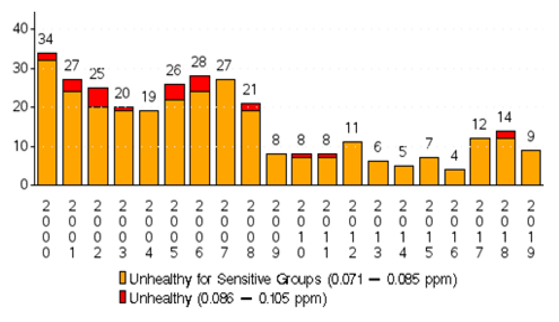
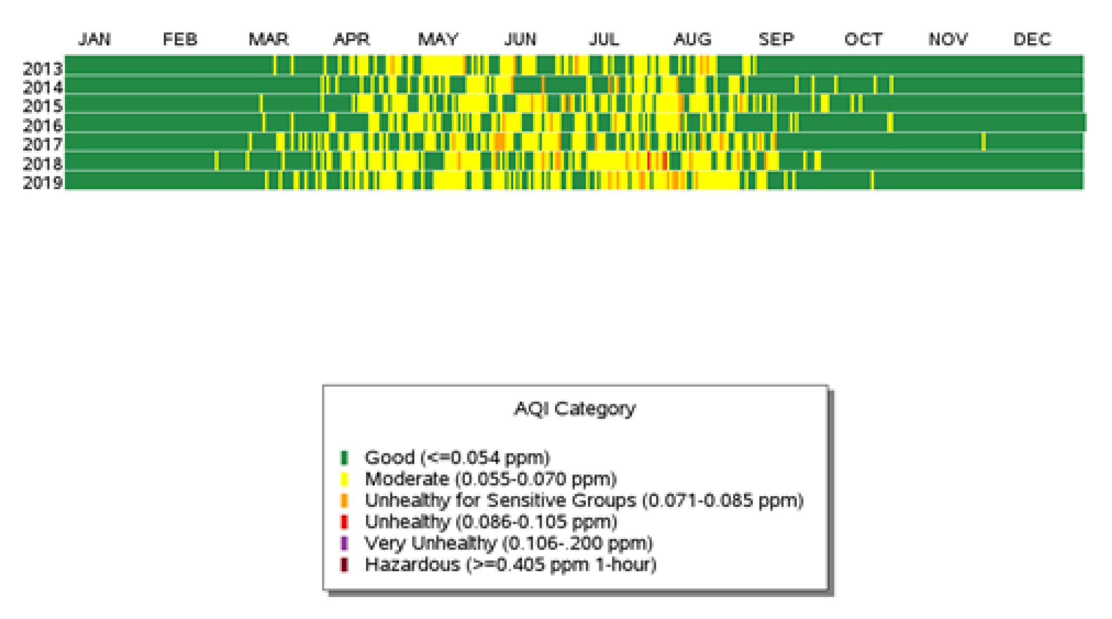
Figure 1 is a representation of the annual high ozone events recorded by the Texas Commission on Environmental Quality (TCEQ) ground stations known as Continuous Ambient Monitoring Stations (CAMS) from 2000 to 2019. In this region, the highest ozone levels are commonly recorded during the summer months of June to August (
Figure 2). High Ozone caused by several reasons such as high degree of temperature (June and July are the peak summer months with an average temperature of 40 degree Celsius) with calms winds (mean value of 4–5 m/s), low relative humidity and high solar radiation (roughly 1.5 Langley/min on average) [
4,
5,
6].
A number of studies have been carried out in order to better understand the chemical and physical processes that cause high ozone concentrations in this study area [
7,
8,
9,
10]. Those studies were mainly focused on chemical composition analysis [
11,
12], the sources, and the physical characteristics [
13] of the ozone episodes. Moreover, the topography of the study area is complex resulting in a forecast and prediction accuracy of air quality models that are less adequate to predict pollutant accurately [
14]. In this paper, we propose a study of the use of machine learning techniques in classifying high or low ozone concentration levels, where highly concentrated ozone(>70 ppb) days are class 1 and low concentration ozone(<70 ppb) days are class 0. The dataset used in this paper was retrieved from TCEQ ground stations CAMS. It contains various meteorological and air pollutants that affect ground-level ozone concentration in the area of our study.
First, this dataset is filled up for further processing and then split into the training set and the testing set. In this paper, machine learning algorithms, such as Naive Bayes, K-Nearest Neighbors, Decision Tree, Stochastic Gradient Descent, and XGBoost, are utilized to predict ground ozone level concentration, and their respective accuracy scores are examined. Based on the results, the XGBoost algorithm scored the highest accuracy with 94.09 percent. The present study evaluates the first predictions of ground ozone using relatively simple predicting techniques. It can be a useful reference for scientists and meteorologists for better forecasting. In addition, the direct comparison of six different algorithms gives machine learning researchers insight into which algorithm produces the most accurate results.
This paper is constructed as follows:
Section 2 describes the machine learning approaches of the six supervised algorithms.
Section 3 presents the data description. The exploratory data analysis is presented in
Section 4 with a focus on combining datasets.
Section 5 describes the numerical experiments carried out on the real-world environment dataset. Conclusions and potential future directions will be discussed in
Section 6.
2. Machine Learning Approach
This section discusses the machine learning techniques such as: Naive Bayes, K-Nearest Neighbors, Decision Tree, Stochastic Gradient Descent, and XGBoost, which were used to classify the ozone data. For this purpose, 70% of the data were applied for training a predictive model, and 30% of the data were used for testing the model based on their tuning parameters.
2.1. Naive Bayes Classifier
Naive Bayes (NB) is a supervised machine learning method, which takes the concept of conditional probability, to classify the target variable. The assumption of Bayes’ theorem is to compute the probability of any class of target variable occurring based on the probability of other features that have already happened. The logic behind the model is using Bayes’ theorem with the assumption of Naive, which has independent features. The model finds the probability of each class of target variables depending on some independent features. The highest probability determines the final class of target variable. The algorithm is pretty fast and is mostly used for discrete data. However, for the continuous data, the NB needs additional assumptions regarding the distribution of features. In this study, we used Gaussian NB for our continuous data (see [
15] for more details).
2.2. k-Nearest Neighbors Algorithm
k-Nearest Neighbor or k-NN is a simple, non-parametric, easy to implement machine learning algorithm based on the supervised learning method. It assumes that each data point is a part of its nearest group or class based on the Euclidean distance metric. So an unclassified data point can be assigned to a class by finding what class is nearest to it. In this case, k is the hyper-parameter (typically, an odd number), that is, the number of nearest data points from unclassified data point.
2.3. Decision Tree Classifier
Decision Tree (DT) Classifiers are supervised machine learning methods that are among the easiest and inexpensive methods to grasp intuitively, due to the incorporation of decision point logic, similar to a flowchart. The inputs can be numeric or categorical. It contains nodes and edges, starting with the root node at a decision point. Edges are one of the possible answers to the question asked by the ‘node’. The records are split until they cannot be split any further. So the classifier process ends when the leaf node is reached, which represents the output value for the prediction. If a separation cannot create a perfect split between the categorical response variable then it is called “impure”. One metric that evaluates the impurity of a split is called “gini”.
Gini impurities are calculated by subtracting from one the probability of one category squared minus the probability of another category squared and so on, as well as for any combination of the categories. These values are calculated for each node and are then aggregated as a weighted average. For numeric data, the values are sorted, and then averages are created using adjacent values and then gini impurities are derived using these. The least impure average is used as a greater than or less than split. Ranked data can be used to create splits as well. A split is chosen if its impurity is the lowest. This process is repeated to make additional splits based on the previous split [
16].
2.4. XGBoost Algorithm
Gradient Boosting (GB) is a supervised algorithm that is used to predict a target variable via an ensemble technique. Chen and Guestrin proposed the Extreme GB (XGboost) algorithm on the basis of the Gradient Boosting Decision Tree (GBDT) structure [
17]. In regular GB, the loss function is used only for the base model (e.g., decision tree) rather than the overall model. As compared to other algorithms, XGboost provides more information about the gradient direction and achieves a minimum of loss function quickly. The reason is that XGboost uses the second order derivative for gradient approximation [
18]. This is a very fast algorithm and has several tuning parameters to improve the model, such as drop rate, sub-sample, ntrees, skip drop, and so forth.
2.5. Stochastic Gradient Descent
Gradient descent is an optimization algorithm used in finding the parameters by minimizing a cost function. The algorithm is usually slow for large datasets. The stochastic gradient descent (SGD) updates the parameters for each training data point. So the frequent updates make the algorithm computationally more expensive compared to the batch gradient descent. However, the SGD algorithm provides with the detailed information for model improvement. A brief overview of the gradient descent algorithm is as follows:
Assume that a hypothesis is
, where the parameters are
. At this point, the cost function is:
The goal is to minimize the cost function
) and to find the optimum parameters
. To do so, we use the gradient descent algorithm:
where
, and
is the learning rate, or how rapidly do we want to move towards the minimum. At this point, a learning rate is specified that controls the amount of change of coefficients on each update. Overshoot can also be done for the case of large
[
19].
2.6. Ensemble Methods
The Ensemble method aggregates the predictions of several similar or conceptually different models built with a given learning algorithm, improving robustness compared to a single model. Voting Classifier is one of the basic ensemble techniques. This approach works like an electoral system, in which a prediction of a new data point is made based on the machine learning models studied. In this study, we used a soft voting system where each classifier’s specific weight is set with the “weight” parameter. As a probability estimate for the loss function of the SGD classifier (‘hinge’) is not available, we used the weights of the other classifiers. The weights were chosen based on the accuracy and other evaluation metrics. We then multiplied the probabilities and weights of each classifier and took the average of all samples. The maximum average probability is used for the final classification.
3. Data Background
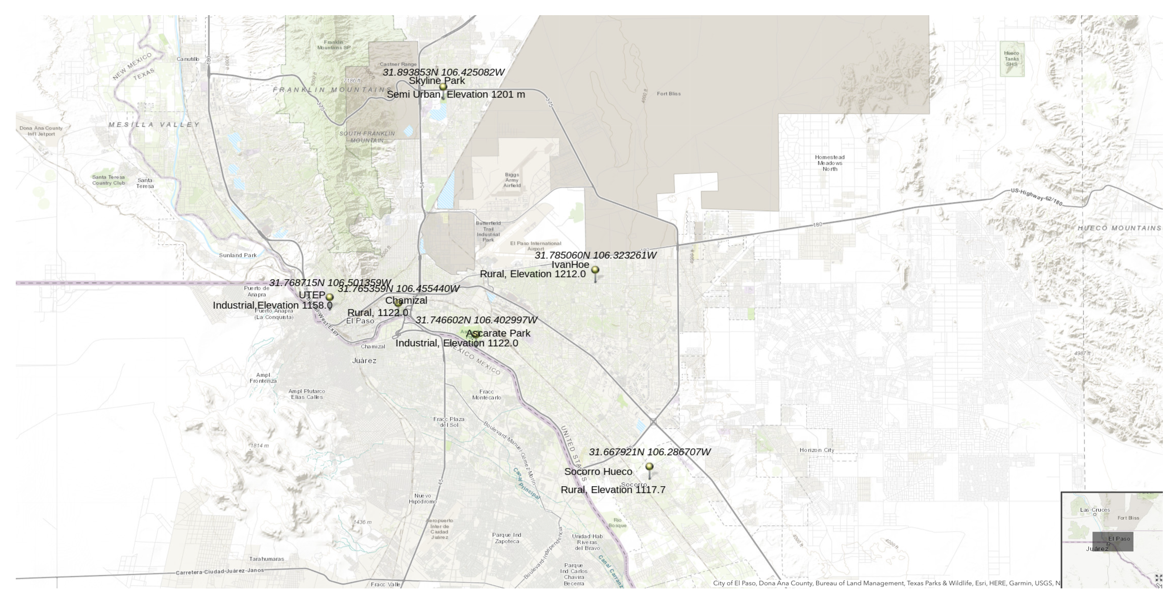
Meteorological and Air pollutant parameters from six different locations of the El Paso area are used to create the database (
Figure 3). Those locations represent all four different parts of the area: Urban, Rural, Industrial and Semi-industrial. El Paso possesses the typical southwestern US urban climate, which is warm and arid with poor air quality, partly due to industrial activity along the US/Mexico border, as well as unique meteorological conditions caused by local geography [
20,
21,
22]. There are approximately 0.7 million people in El Paso, with 1.3 million in Cuidad Juarez, Mexico, immediately adjacent to El Paso (Padgett and Thomas, 2001). El Paso is often found to be in non-attainment of the US National Ambient Air Quality Standards (NAAQS) for
, CO,
, and
. This non-attainment is due to the combination of a high population concentration, industrial influences, and weather conditions [
23].
To capture the full topographic and meteorological characteristics of this study area, data from six different stations were used. Detailed information about these monitoring stations is given below in the following
Table 1.
4. Exploratory Data Analysis
In this study, data are collected from CAMS administered by TCEQ. An average of ground-level Ozone concentrations from the six stations of monitoring stations in El Paso is provided.
As can be interpreted from
Figure 4, most of the high ozone days occurred in the summer season. Minimum values of ozone days took place in January as the temperature has a positive correlation with ozone concentration. From the month of May–August, high ozone days are ubiquitous in our area of study with exceeding values from the NAAQS standard.
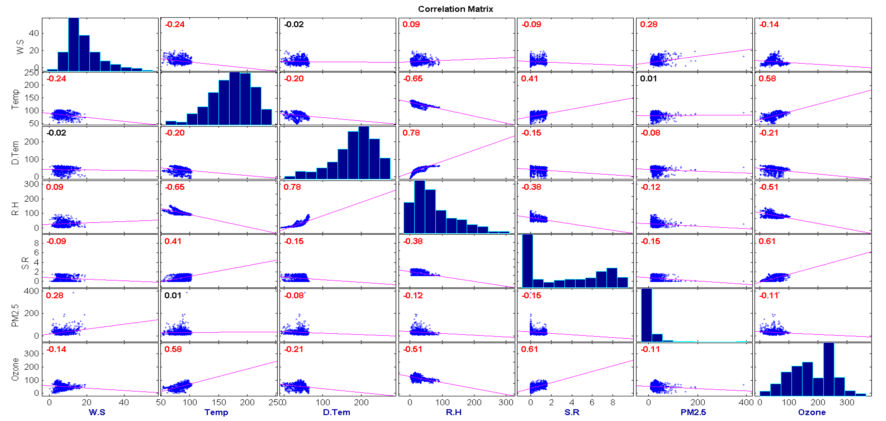
In
Figure 5, a correlation matrix for all the different variables with ozone is presented. The relationship between Ozone and Temperature is positively correlated and ranging the value around 0.60. Meanwhile, the relation between Relative Humidity, Solar Radiation with Ozone is negatively correlated as the value ranges around (−0.5) to (−0.6).
Table 2 represents the descriptive statistics of independent variables, which includes mean, median, standard deviation, minimum values, first quartile, second quartile, third quartile and maximum values. All the fractional values are rounded to two digits after the decimal point.
5. Results & Discussion
This section will illustrate some experimental results of six machine learning techniques applied to our dataset.
5.1. Analysis of Fitted Models
We first analyzed the NB Classifier to create a predictive model using training data points. The NB Classifier can be highly scaled with the predictors and it requires a low number of data points. It is observed that NB is robust to the outlier and irrelevant features of data. We then used the k-NN algorithm that worked based on the parameter k. The k-NN classifier is very sensitive to the low values of k, leading to high variance and low bias of the model. On the other hand, if we take the large values of k, the model leads to low variance and high bias. Using cross-validation, we found that k = 5 fits well with our trained data. The decision tree algorithm does not require any scaling or normalization of our trained data. We also used the gini index to identify the important variables. Using the XGBoost algorithm, we obtained 94.09% accuracy on the test data, which is the highest accuracy among the algorithms. In this case, the in-built Lasso and Ridge Regression regularization were used to prevent the model from overfitting. The algorithm also comes with a built-in capability to handle missing values. In the SGD algorithm, we updated the weights based on each training example, not the batch as a whole. Hence, it updates the parameters for each training example one by one. The SGD approach reaches convergence much faster than batch gradient descent since it updates weights using a single data point in each iteration. So the curve of cost versus epoch for SGD algorithm is not smooth. The predictive results are shown in Tables 7 and 8 and Figures 7 and 8.
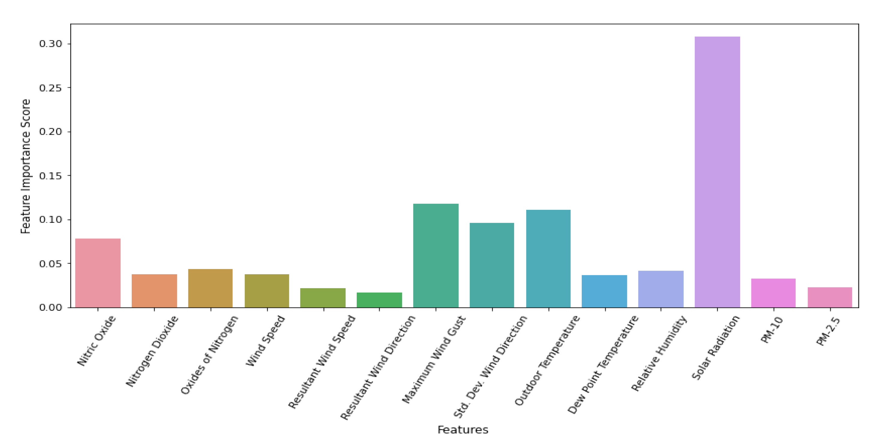
5.2. Feature Selection
The feature importance enables the machine learning algorithm to train faster, reduces the computational cost (and time) of training, and makes it simpler to interpret. It also reduces the variance of the model and improves the accuracy if the right subset is chosen. In this paper, we used different measures to select the right features (see
Table 3 and
Table 4 and
Figure 6). At this point, the ensemble model does not provide the coefficients of features due to the NB classifier. Thus, we present the coefficients of the nearest accurate model, that is, XGBoost.
The significance level and the
p-values of predictors obtained from the Ordinary Least Squares [
24] method are also employed in this study. The significance level (0.05) is the amount of change a feature will affect towards the final output and the
p-value is the hypothesis of the significance level. At this point, the null hypothesis refers to the predictors of the model that are not significant. The higher the
p-value is, the less important the feature is. From
Table 4, it is clear that Nitric Oxide, Oxides of Nitrogen, Resultant Wind Direction,
, and
are not important predictors, as the
p-values are higher than the significance level. Thus, these features do not alter the classification and can be easily removed without causing any problems. On the other hand, Solar Radiation is most significant on days that are high in ozone. However, the Ordinary Least Square usually does not provide a good estimation for high dimensional datasets, thus we performed other machine learning processes to select important features (see
Table 3 and
Figure 6).
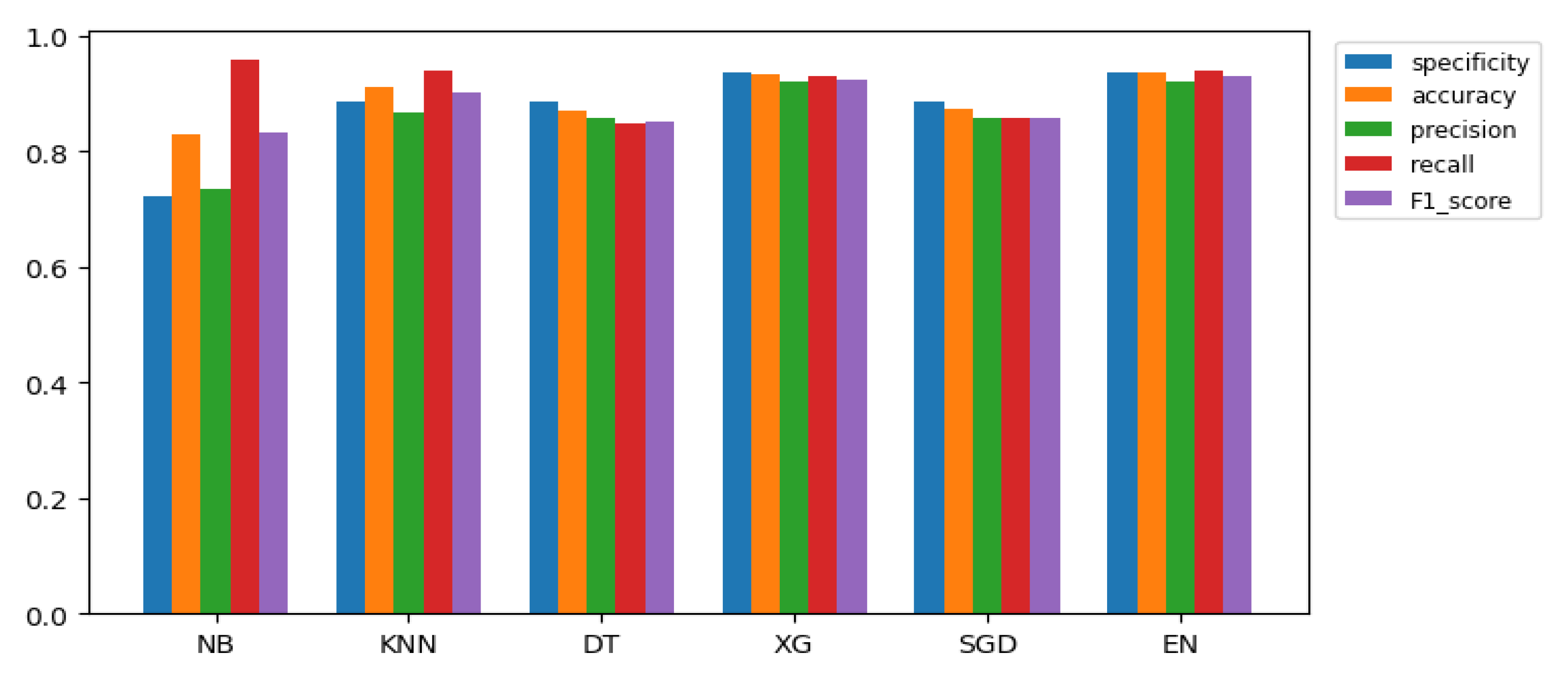
5.3. Model Evaluation
Table 5 and
Table 6 show that the predicted Mean Squared Error and Misclassification Rate of the models are very low for the dataset.
In this section, we ensemble all the methods used in this paper and present their accuracy.
Table 7 and
Table 8 and
Figure 7 and
Figure 8 show the specificity, accuracy, precision, recall, and F1 score of the models.
Specificity is used to measure the predictive performance of the classification models. Specificity informs us about the proportion of actual negative cases that our model has predicted as negative. Here, the highest value of specificity is 94.26%, which means that the Ensemble model we used is good at predicting the true negatives. To fully evaluate the effectiveness of a model, we must examine both precision and recall. Precision measures the percentage of ozone labeled as high that were correctly classified. On the other hand, recall measures the percentage of actual ozone labels that were correctly classified. F1 score is the harmonic mean of precision and recall. In this study, we also used the F1 score as an evaluation metric. The reason is that the percentage of accuracy can sometimes be disproportionately skewed by a large number of actual negatives (low ozone level) results.
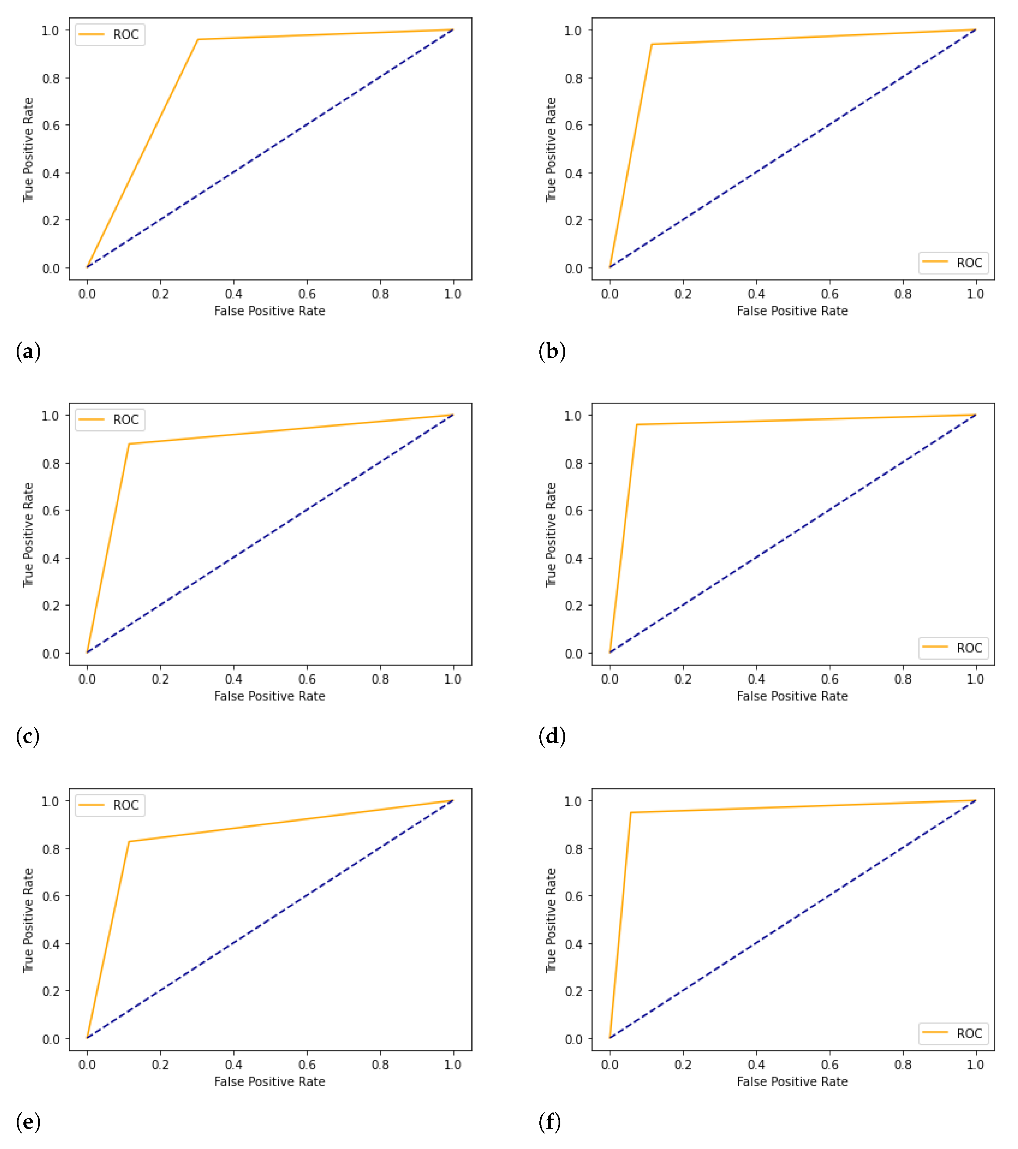
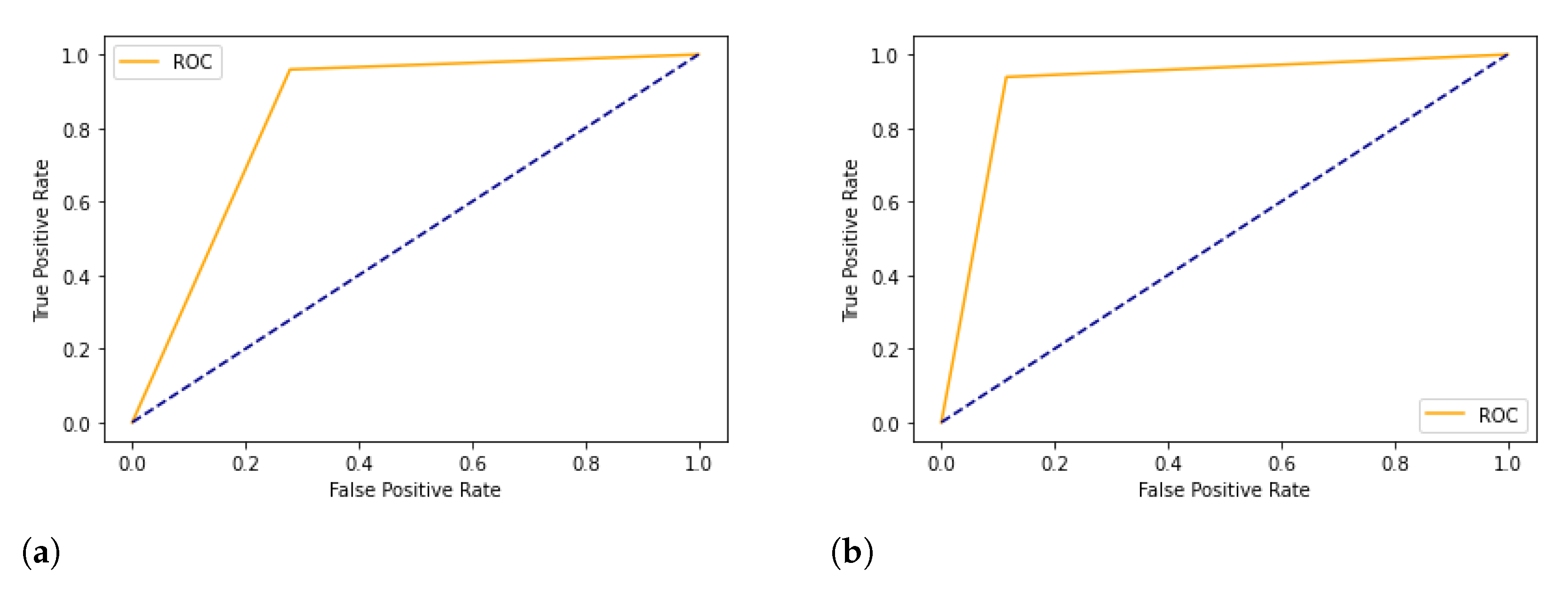
We plotted the ROC curve between True Positive Rate (X-axis) and False Positive Rate (Y-axis). In
Figure 9 and
Figure 10, the diagonal line represents the threshold of the ROC curve. We see that the Ensemble model has good accuracy, precision, recall, F1 score, and area under the ROC curve.
6. Conclusions
The study presented here is an extended version of analyzing machine learning for the classification of ozone in the Paso del Norte region [
25]. In this case, we explore six different machine learning models in the El Paso area, in order to classify the ozone concentration in a bi-national area. In comparison to previous works in this region, this work mainly focuses on the ensemble of machine learning algorithms and study area. The algorithms used in the study are Naive Bayes, K-Nearest Neighbors, Decision Tree, Stochastic Gradient Descent, and XGBoost. The Ensemble methods have also been used to classify the ozone level. The dataset contains a mix of several air pollutants and meteorological parameters.
Initially, we did the exploratory data analysis to pre-process the data and analyze the correlation of predictors. The machine learning models have been trained with training data to build a predictive model. The performance of the predictive models has been measured by the evaluation metrics such as Mean Squared Error, Misclassification Rate, Accuracy, Specificity, Precision, Recall, and F1 Score. The XGBoost model and p-values of predictors from the OLS technique are used to determine the important variables that are useful in detecting high or low ozone days.
The Ensemble Method was able to predict 94.55% of ozone observations with high or low levels. The results indicate that the high concentration of ozone is highly influenced by Nitric Oxide, Nitrogen Dioxide, Oxides of Nitrogen, Wind Speed, Maximum Wind Gust, Std. Dev. Wind Direction, Outdoor Temperature, Relative Humidity, and Solar Radiation (see
Table 3 and
Table 4 and
Figure 6).
Author Contributions
M.A.M.B. and S.M. contributed to the supervision and project administration, M.A.M.B., R.K.S., M.R.I., and S.M., contributed to the conceptualization, methodology, and result analysis. All authors have read and agreed to the published version of the manuscript.
Funding
This research was funded by Austin Peay State University.
Acknowledgments
The authors like to thank the Texas Commission of Environmental Quality and Atmospheric Physics Lab (UTEP) for all their support.
Conflicts of Interest
The authors declare no conflict of interest.
References
- Lee, S.H.; Kim, S.W.; Angevine, W.M.; Bianco, L.; McKeen, S.A.; Senff, C.J.; Zamora, R.J. Evaluation of urban surface parameterizations in the WRF model using measurements during the Texas Air Quality Study 2006 field campaign. Atmos. Chem. Phys. 2011, 11, 2127. [Google Scholar] [CrossRef] [Green Version]
- Pernak, R.; Alvarado, M.; Lonsdale, C.; Mountain, M.; Hegarty, J.; Nehrkorn, T. Forecasting Surface O3 in Texas Urban Areas Using Random Forest and Generalized Additive Models. Aerosol Air Qual. Res. 2019, 19, 2815–2826. [Google Scholar] [CrossRef]
- Part, V. Federal Register Document. Fed. Regist. 1997, 62, 38855–38896. [Google Scholar]
- Seila, R.L.; Main, H.H.; Arriaga, J.L.; Martnez, G. Atmospheric volatile organic compound measurements during the 1996 Paso del Norte Ozone Study. Sci. Total. Environ. 2001, 276, 153–169. [Google Scholar] [CrossRef]
- Mahmud, S.; Karle, N.N.; Fitzgerald, R.M.; Lu, D.; Nalli, N.R.; Stockwell, W.R. Intercomparison of Sonde, WRF/CAMx and Satellite Sounder Profile Data for the Paso Del Norte Region. Aerosol Sci. Eng. 2020, 4, 277–292. [Google Scholar] [CrossRef]
- Karle, N.N.; Mahmud, S.; Sakai, R.K.; Fitzgerald, R.M.; Morris, V.R.; Stockwell, W.R. Investigation of the Successive Ozone Episodes in the El Paso–Juarez Region in the Summer of 2017. Atmosphere 2020, 11, 532. [Google Scholar] [CrossRef]
- Brown, M.J.; Muller, C.; Wang, G.; Costigan, K. Meteorological simulations of boundary-layer structure during the 1996 Paso del Norte Ozone Study. Sci. Total. Environ. 2001, 276, 111–133. [Google Scholar] [CrossRef]
- Einfeld, W.; Church, H.W.; Yarbrough, J.W. Winter Season Air Pollution in El Paso-Ciudad Juarez; United States Environmental Protection Agency, Region VI, Air, Pesticides Toxics Division: Washington, DC, USA, 1995.
- Funk, T.H.; Chinkin, L.R.; Roberts, P.T.; Saeger, M.; Mulligan, S.; Figueroa, V.P.; Yarbrough, J. Compilation and evaluation of a Paso del Norte emission inventory. Sci. Total. Environ. 2001, 276, 135–151. [Google Scholar] [CrossRef]
- Ordieres, J.B.; Vergara, E.P.; Capuz, R.S.; Salazar, R.E. Neural network prediction model for fine particulate matter (PM2.5) on the US–Mexico border in El Paso (Texas) and Ciudad Juárez (Chihuahua). Environ. Model. Softw. 2005, 20, 547–559. [Google Scholar] [CrossRef]
- Shi, C.; Fernando, H.J.S.; Yang, J. Contributors to ozone episodes in three US/Mexico border twin-cities. Sci. Total. Environ. 2009, 407, 5128–5138. [Google Scholar] [CrossRef] [PubMed]
- Zora, J.E.; Sarnat, S.E.; Raysoni, A.U.; Johnson, B.A.; Li, W.W.; Greenwald, R.; Sarnat, J.A. Associations between urban air pollution and pediatric asthma control in El Paso, Texas. Sci. Total. Environ. 2013, 448, 56–65. [Google Scholar] [CrossRef] [PubMed]
- Mahmud, S. Optimization of Regional Scale Numerical Weather Prediction & Air Quality Model for the Paso Del Norte Region. Ph.D. Thesis, The University of Texas at El Paso, El Paso, TX, USA, 2020. [Google Scholar]
- Mahmud, S. The Use of Remote Sensing Technologies and Models to Study Pollutants in the Paso del Norte Region; The University of Texas at El Paso: El Paso, TX, USA, 2016. [Google Scholar]
- Moraes, R.M.; Machado, L.S. Gaussian naive bayes for online training assessment in virtual reality-based simulators. Mathw. Soft Comput. 2009, 16, 123–132. [Google Scholar]
- Pandya, R.; Pandya, J. C5. 0 algorithm to improved decision tree with feature selection and reduced error pruning. Int. J. Comput. Appl. 2015, 117, 18–21. [Google Scholar] [CrossRef]
- Chen, T.; Guestrin, C. Xgboost: A scalable tree boosting system. In Proceedings of the 22nd ACM Sigkdd International Conference on Knowledge Discovery and Data Mining, San Francisco, CA, USA, 13–17 August 2016; pp. 785–794. [Google Scholar]
- Quinto, B. Next-Generation Machine Learning with Spark; Springer: Berlin, Germany, 2020. [Google Scholar]
- Stochastic Gradient Descent. Available online: https://en.wikipedia.org/wiki/Stochastic-gradient-descent (accessed on 23 September 2021).
- MacDonald, C.P.; Roberts, P.T.; Main, H.H.; Dye, T.S.; Coe, D.L.; Yarbrough, J. The 1996 Paso del Norte Ozone Study: Analysis of meteorological and air quality data that influence local ozone concentrations. Sci. Total Environ. 2001, 276, 93–109. [Google Scholar] [CrossRef]
- Mahmud, S.; Wangchuk, P.; Fitzgerald, R.; Stockwell, W. Study of Photolysis rate coefficients to improve air quality models. Bull. Am. Phys. Soc. 2016, 61, 15. [Google Scholar]
- Fujita, E.M. Hydrocarbon source apportionment for the 1996 Paso del Norte Ozone Study. Sci. Total. Environ. 2001, 276, 171–184. [Google Scholar] [CrossRef]
- Mahmud, S.; Bhuiyan, M.A.M.; Sarmin, N.; Elahee, S. Study of wind speed and relative humidity using stochastic technique in a semi-arid climate region. AIMS Environ. Sci. 2020, 7, 156–173. [Google Scholar] [CrossRef]
- Pavelescu, F.M. Features Of The Ordinary Least Square (Ols) Method. Implications for the Estimation Methodology. J. Econ. Forecast. 2004, 1, 85–101. [Google Scholar]
- Bhuiyan, M.A.M.; Mahmud, S.; Sarmin, N.; Elahee, S. A Study on Statistical Data Mining Algorithms for the Prediction of Ground-Level Ozone Concentration in the El Paso–Juarez Area. Aerosol Sci. Eng. 2020, 4, 293–305. [Google Scholar] [CrossRef]
Figure 1.
Total number of days with 8-hr daily ozone exceedance (above 70 ppbv) during the years of 2000–2019 in El Paso, Texas.
Figure 1.
Total number of days with 8-hr daily ozone exceedance (above 70 ppbv) during the years of 2000–2019 in El Paso, Texas.
Figure 2.
Ozone daily Air Quality Index (AQI) values from 2013 to 2019 for all the CAMS stations in El Paso, Texas.
Figure 2.
Ozone daily Air Quality Index (AQI) values from 2013 to 2019 for all the CAMS stations in El Paso, Texas.
Figure 3.
Six ozone monitoring stations in El Paso and their geographic centroid.
Figure 3.
Six ozone monitoring stations in El Paso and their geographic centroid.
Figure 4.
Daily (maximum 8 h) ozone concentration from all the stations of the study area, (a) Ivanhoe, (b) El Paso (UTEP), (c) Chamizal, (d) Ascarate Park, (e) Socorro Hueco, and (f) Skyline park.
Figure 4.
Daily (maximum 8 h) ozone concentration from all the stations of the study area, (a) Ivanhoe, (b) El Paso (UTEP), (c) Chamizal, (d) Ascarate Park, (e) Socorro Hueco, and (f) Skyline park.
Figure 5.
Correlation matrix for the dataset.
Figure 5.
Correlation matrix for the dataset.
Figure 6.
Visual representation of feature importance.
Figure 6.
Visual representation of feature importance.
Figure 7.
Model performance for Ozone dataset.
Figure 7.
Model performance for Ozone dataset.
Figure 8.
Model performance with selected feature for Ozone dataset.
Figure 8.
Model performance with selected feature for Ozone dataset.
Figure 9.
ROC Curve for Ozone dataset. (a) Fitted Naive Bayes; (b) Fitted K-Nearest Neighbors; (c) Fitted Decision Tree; (d) Fitted XGBoost; (e) Fitted Stochastic Gradient Descent; (f) Fitted Ensemble.
Figure 9.
ROC Curve for Ozone dataset. (a) Fitted Naive Bayes; (b) Fitted K-Nearest Neighbors; (c) Fitted Decision Tree; (d) Fitted XGBoost; (e) Fitted Stochastic Gradient Descent; (f) Fitted Ensemble.
Figure 10.
ROC Curve for selected featured Ozone dataset. (a) Fitted Naive Bayes; (b) Fitted K-Nearest Neighbors; (c) Fitted Decision Tree; (d) Fitted XGBoost; (e) Fitted Stochastic Gradient Descent; (f) Fitted Ensemble.
Figure 10.
ROC Curve for selected featured Ozone dataset. (a) Fitted Naive Bayes; (b) Fitted K-Nearest Neighbors; (c) Fitted Decision Tree; (d) Fitted XGBoost; (e) Fitted Stochastic Gradient Descent; (f) Fitted Ensemble.
Table 1.
Ozone monitoring stations.
Table 1.
Ozone monitoring stations.
| Station | Lat/Lon | Elevation | Type |
|---|
| C12 UTEP | 31.7682/−106.5012 | 1158.0 | Industrial |
| C37 Ascarate Park | 31.7467/−106.4028 | 1122.0 | Industrial |
| C41 Chamizal | 31.7656/−106.45522 | 1122.0 | Rural |
| C49 Socorro Hueco | 31.6675/−106.2880 | 1117.7 | Rural |
| C72 Skyline Park | 31.8939/−106.4258 | 1201.0 | Semi Urban |
| C414 Ivanhoe | 31.7857/−106.3235 | 1212.0 | Rural |
Table 2.
Descriptive statistics of data.
Table 2.
Descriptive statistics of data.
| Features | Mean | Median | STD | Min | 1st Q | 2nd Q | 3rd Q | Max |
|---|
| Nitric Oxide | 0.93 | 0.40 | 2.68 | −1.1 | 0 | 0.4 | 0.8 | 31.8 |
| Nitrogen Dioxide | 8.66 | 6.70 | 7.07 | −1.1 | 4.45 | 6.7 | 10.5 | 54.8 |
| Oxides of Nitrogen | 9.43 | 7.00 | 8.85 | −1.6 | 4.6 | 7 | 11.1 | 75.1 |
| Wind Speed | 5.76 | 5.10 | 3.88 | 1.6 | 4.2 | 5.1 | 6.4 | 68 |
| Resultant Wind Speed | 4.41 | 3.80 | 3.7 | 0.2 | 2.5 | 3.8 | 5.6 | 79 |
| Resultant Wind Direction | 151.07 | 126.00 | 84.79 | 0 | 96 | 126 | 196.5 | 360 |
| Maximum Wind Gust | 13.48 | 12.60 | 5.78 | 3.2 | 10.5 | 12.6 | 14.9 | 76 |
| Std. Dev. Wind Direction | 37.97 | 37.00 | 17.3 | 10 | 21 | 37 | 51 | 87.4 |
| Outdoor Temperature | 89.73 | 91.10 | 8.04 | 32 | 85.25 | 91.1 | 95.2 | 107.1 |
| Dew Point Temperature | 42.92 | 42.80 | 9.26 | 16.8 | 36.25 | 42.8 | 48.95 | 89.4 |
| Relative Humidity | 22.16 | 18.90 | 13.38 | 0 | 13.2 | 18.9 | 24.8 | 86.6 |
| Solar Radiation | 0.64 | 0.51 | 1.12 | 0 | 0 | 0.51 | 1.17 | 20.4 |
| 31.37 | 25.30 | 43.22 | −5.9 | 19.4 | 25.3 | 34.4 | 906 |
| 10.86 | 8.00 | 12.26 | −3 | 5.3 | 8 | 11.2 | 146 |
Table 3.
Coefficients for important feature using XGboost.
Table 3.
Coefficients for important feature using XGboost.
| Features | Coefficients |
|---|
| Nitric Oxide | 0.077 |
| Nitrogen Dioxide | 0.037 |
| Oxides of Nitrogen | 0.043 |
| Wind Speed | 0.037 |
| Maximum Wind Gust | 0.117 |
| Std. Dev. Wind Direction | 0.096 |
| Outdoor Temperature | 0.110 |
| Dew Point Temperature | 0.036 |
| Relative Humidity | 0.041 |
| Solar Radiation | 0.307 |
Table 4.
Analysis of feature importance using p-values.
Table 4.
Analysis of feature importance using p-values.
| Features | p-Values |
|---|
| Nitric Oxide | 10 |
| Nitrogen Dioxide | |
| Oxides of Nitrogen | |
| Wind Speed | |
| Resultant Wind Speed | |
| Maximum Wind Gust | |
| Std. Dev. Wind Direction | |
| Outdoor Temperature | |
| Dew Point Temperature | |
| Relative Humidity | |
| Solar Radiation | |
| |
| |
Table 5.
Model Evaluation for Ozone dataset.
Table 5.
Model Evaluation for Ozone dataset.
| Models | Mean Squared Error | Misclassification Rate |
|---|
| NB | 0.186 | 0.186 |
| KNN | 0.1 | 0.1 |
| DT | 0.118 | 0.118 |
| XG | 0.059 | 0.059 |
| SGD | 0.141 | 0.141 |
| EN | 0.055 | 0.055 |
Table 6.
Model Evaluation for selected features of Ozone dataset.
Table 6.
Model Evaluation for selected features of Ozone dataset.
| Models | Mean Squared Error | Misclassification Rate |
|---|
| NB | 0.173 | 0.173 |
| KNN | 0.091 | 0.091 |
| DT | 0.132 | 0.132 |
| XG | 0.068 | 0.068 |
| SGD | 0.127 | 0.127 |
| EN | 0.064 | 0.064 |
Table 7.
Model Evaluation metrics analysis for Ozone dataset.
Table 7.
Model Evaluation metrics analysis for Ozone dataset.
| Models | Specificity | Accuracy | Precision | Recall | F1 Score |
|---|
| | (%) | (%) | (%) | (%) | [0, 1] |
|---|
| NB | 69.67 | 81.36 | 71.75 | 95.91 | 0.82 |
| KNN | 88.52 | 90 | 86.54 | 91.84 | 0.89 |
| DT | 88.52 | 88.18 | 86 | 87.76 | 0.87 |
| XG | 92.62 | 94.09 | 91.26 | 95.92 | 0.94 |
| SGD | 88.52 | 85.91 | 85.26 | 82.65 | 0.84 |
| EN | 94.26 | 94.55 | 93.0 | 94.90 | 0.94 |
Table 8.
Evaluation metrics analysis for selected feature of Ozone dataset.
Table 8.
Evaluation metrics analysis for selected feature of Ozone dataset.
| Models | Specificity | Accuracy | Precision | Recall | F1 Score |
|---|
| | (%) | (%) | (%) | (%) | [0, 1] |
|---|
| NB | 72.13 | 82.72 | 73.44 | 95.92 | 0.83 |
| KNN | 88.52 | 90.1 | 86.79 | 93.87 | 0.90 |
| DT | 88.52 | 86.81 | 85.57 | 84.69 | 0.85 |
| XG | 93.44 | 93.18 | 91.92 | 92.86 | 0.92 |
| SGD | 88.52 | 87.27 | 85.71 | 85.71 | 0.86 |
| EN | 93.44 | 93.64 | 92 | 93.87 | 0.93 |
| Publisher’s Note: MDPI stays neutral with regard to jurisdictional claims in published maps and institutional affiliations. |
© 2021 by the authors. Licensee MDPI, Basel, Switzerland. This article is an open access article distributed under the terms and conditions of the Creative Commons Attribution (CC BY) license (https://creativecommons.org/licenses/by/4.0/).


