Thermo-Optical Mechanical Waves in a Rotating Solid Semiconductor Sphere Using the Improved Green–Naghdi III Model

Abstract

The current study investigates thermophotovoltaic interactions using a new mathematical model of thermoelasticity established on a modification of the Green–Naghdi model of type III (GN-III). The basic equations, in which the heat transfer is in the form of the Moore–Gibson–Thompson (MGT) equation, are derived by adding a single delay factor to the GN-III model. The impact of temperature and electrical elastic displacement of semiconductors throughout the excited thermoelectric mechanism can be studied theoretically using this model. The proposed model was used to investigate the interactions between the processes of thermoelastic plasma in a rotating semiconductor solid sphere that was subjected to a thermal shock and crossed to an externally applied magnetic field. The influence of rotation parameters on various photothermal characteristics of silicon solid was presented and explored using the Laplace technique.

1. Introduction

Several developments have been made in the field of ultrafast carrier dynamics in semiconductor materials during the last five decades. The motives for the study include not only basic scientific interests, but also the application of semiconductor optoelectronic and electronic devices and the growing need for faster interaction and information processing. To continuously improve microelectronic semiconductor devices, various dynamic processes in semiconductors must be understood. As a result, the excitation of semiconductors to the disequilibrium state, as well as the numerous relaxation processes that follow, must be thoroughly investigated.

The photoacoustic (PA) signal can be detected on the front side of a material that has been irradiated with a modulated optical beam or on the back side of a material that has been irradiated with an unmodulated optical beam. The heat-transmission detection system may be used for a variety of applications, including the assessment of heat propagation mechanisms in solid materials [1]. When this approach is used for semiconductors, it is possible to obtain additional information about carrier transport properties [2]. Because of the periodic generation of excess carriers into semiconductors, the carrier thermalization and recombination processes will produce thermal waves. The semiconductor materials experience mechanical stress when electron-hole pairs occur.

The sound wave is formed when photo-induced free carriers induce periodic elastic strain in the material [3]. The semiconductor coefficients are also influenced by the carrier density, however, the effect is small [4]. Some materials, such as semiconductors, offer a variety of physical features that might aid research. The concept of thermoelasticity only allows semiconductor materials to be classified as elastic materials. The significance of semiconductors in technological advancement was recently highlighted when they were utilized to create electrical energy of sunlight, even when being subjected to ultrasound [5]. Superconductors are nanoparticles utilized in electrical and electronic engineering, and have a wide range of uses in contemporary industry, including transistors, displays, and solar cells.

The concept of photovoltaic energy has only recently been introduced into semiconductor media in order to generate alternative energy sources. To determine the relationship between the photothermal equations and thermoelasticity, a number of theoretical models have been examined. Gordon et al. [6] first used electronic displacements in a photo-thermal spectroscopic. Photoacoustic spectroscopy [7] is a specific and sensitive method that uses a laser source to determine the acoustic velocity of a type of semiconductor.

In photothermal processing techniques, wave propagation is used in many applications in today’s engineering industries during electro-deformations of elastic semiconductor material [8]. Abouelregal [9] investigated the responses in a solid, rotating semiconductor cylinder because of changing heat flow. Abouelregal et al. [10,11,12] studied the impact of an additional carrier on a semiconducting spinning half-space exposed to a normal force using the Green and Naghdi models.

Due to the more realistic predictions from the theory of uncoupled or coupled thermoelasticity, interest is growing these days in theories of extended thermoelasticity. The phenomenon of the unlimited speed of heat transmission inherent in the classical coupled thermoelasticity theory is being addressed by modified generalized theories [13,14,15,16] developed during the last five decades. Green and Naghdi [17,18,19] presented Green–Naghdi models (type II and III) as alternative expanded models for thermoelasticity with or without energy dissipation. The type II model does not allow for energy dissipation and is thus regarded as a special case of type III, which does allow for energy dissipation.

Numerous scholarly publications devoted to the study and interpretation of the MGT equation have emerged in recent years. The theory also focuses on third-order governing equations, which are useful in many applications of fluid mechanics [20]. Quintanilla [21,22] is developing a new MGT heat conduction model. After adding the relaxation parameter to the GN-III model, Abouelregal et al. [23,24,25] developed the suggested modified heat equation and employed the energy equation. Since the MGT equation was introduced, the number of papers on this idea has exploded [26,27,28,29]. Other results on bodies with the microstructure can be found in the papers [30,31,32,33].

Several authors have used classical models to investigate the uncoupled and coupled systems of photo-thermoelastic equations and the impacts on semiconductors. A survey of the literature found that there is no study on the volatile evaluation of semiconductor materials subjected to heat and optical loading as well as the temperature-dependent properties of materials. Among the many applications of surface waves in organic semiconductors are nuclear sciences, manufacturing engineering, electric utilities, subsea constructions, compressed gases, aircraft, chemical vessels, and metals, to name a few.

For the first time in this paper, the photothermal MGT heat conduction model (MGTPT), which describes photo-excited carriers and acoustic waves in semiconductors, are introduced. In temporal evolutions of a mainly hyperbolic nature, these equations are of the third order. Due to the presence of the thermal relaxation coefficient in front of the third-order time derivative, the MGTPT model allows for the limited rate of heat spread. To the best of our knowledge, photothermal waves along the interface of semiconducting materials have not been studied before using the MGTPT model.

The Moore–Gibson–Thompson (MGTPT) photothermal heat conduction equation is used to investigate effects throughout photothermal processes in an isotropic, homogeneous, thermoelastic semiconductor solid sphere. The analytical solution is found using numerical inversion methods, and the governing equations, including associated plasmas, thermal processes, and elastic waves, are provided in the field of Laplace transforms. Physical field variables and some analytic comparisons are shown and graphed analytically. The findings were compared to the findings of the study conducted by the researchers.

2. Formulating Mathematical Modeling

Thermoelastic and electronic deformation processes provide the following motion equations with an external force:

$${\sigma }_{ij,j}+F_i=\varrho \ddot{u_i}.$$

(1)

Relationships between constitutive and strain-displacement:

$$\begin{array}{c}{\sigma }_{ij}=C_{ijkl}{e}_{kl}-\left({\beta }_{ij}\theta +d_{nij}N\right).\\ e_{ij}=\frac{1}{2}\left(u_{i,j}+u_{j,i}\right). \end{array}$$

(2)

If the medium rotates at an angular velocity $\overrightarrow{\mathsf{\Omega }}=\mathsf{\Omega } \overrightarrow{\mathrm{n}}$ uniformly, $\overrightarrow{\mathrm{n}}$ being the axis direction of the rotation unit vector, the equation of motion (1) in the rotating reference frame includes two further terms (forces). The centripetal acceleration force $\varrho \overrightarrow{\mathsf{\Omega }}\times (\overrightarrow{\mathsf{\Omega }}\times \overrightarrow{\mathrm{u}})$ is an extra initial term, while the second term is related to time-varying motion and Corioli’s acceleration $2\varrho (\overrightarrow{\mathsf{\Omega }}\times \overrightarrow{\dot{\mathrm{u}}})$. Then, in a rotating reference frame, the equation of motion may be expressed as [25]:

$$\begin{array}{c}{\sigma }_{ij,j}+F_i=\varrho \ddot{u_i}+\varrho \overrightarrow{\mathsf{\Omega }}\times {(\overrightarrow{\mathsf{\Omega }}\times \overrightarrow{\mathrm{u}})}_i+2\varrho {(\overrightarrow{\mathsf{\Omega }}\times \overrightarrow{\dot{\mathrm{u}}})}_i \\ =\varrho \ddot{u_i}+2\rho {(\overrightarrow{\mathsf{\Omega }}\times \overrightarrow{\dot{\mathrm{u}}})}_i+\varrho {[(\overrightarrow{\mathsf{\Omega }}·\overrightarrow{\mathrm{u}})\overrightarrow{\mathsf{\Omega }}-{\mathsf{\Omega }}^2\overrightarrow{\mathrm{u}}]}_i.\end{array}$$

(3)

The corresponding plasma-thermal-elastic wave equation for the increase in carrier density $N$ is as follows [34,35,36]

$${\left(D_{Eij}{N}_{,j}\right)}_{,i}=\varrho \frac{\partial N}{\partial t}+\frac{1}{\tau }N+\kappa \theta +G,$$

(4)

Vasilev and Sandomirskii [36] note that the coupled factor with thermal activation is minimal at lower temperatures when working with a harmonic modification laser.

The conventional Fourier law predicts that propagation speeds will never be infinite. A slight change in the beginning data may be demonstrated to influence the full solution throughout the entire space using this structure. Cattaneo-Vernotte developed a broader Fourier law in [37,38], by adding thermal relaxation ${\tau }_0$ to the heat flow vector $\overrightarrow{q}$ as

$$\left(1+{\tau }_0 \frac{\partial }{\partial t}\right)\overrightarrow{q}=-K_{ij}\overrightarrow{\nabla }\theta .$$

(5)

The thermal relaxation parameter (single delay) ${\tau }_0$ is known as the material-dependent constant, and it is an important element of this research. In terms of physics, the parameter ${\tau }_0$ is the time it takes for a volume element to achieve constant heat conductivity after being exposed to a temperature gradient. This time lag may be translated into a variety of phenomena and contexts, such as when models are used to explore lithotripsy, thermal therapy, ultrasonic cleaning, and high-frequency ultrasound sonochemistry (HFU).

Based on the GN-III type, the Fourier law may be written as [18]

$$\overrightarrow{q}=-K_{ij} \overrightarrow{\nabla }\theta -K_{ij}^{*} \overrightarrow{\nabla }\vartheta ,$$

(6)

where $\vartheta$ represents a thermal displacement that fulfills $\dot{\vartheta }=\theta$, and $K_{ij}^{*}$ signify the rates of the thermal conductivity. The equation of balance energy may be expressed as [39,40]

$$\varrho C_E\frac{\partial \theta }{\partial t}+T_0\frac{\partial }{\partial t}\left({\beta }_{ij}{e}_{ij}\right)=-\overrightarrow{\nabla }·\overrightarrow{q}+Q.$$

(7)

The energy Equation (7), when combined with the enhanced Fourier law presented in (6), has the same flaw as Fourier’s normal model, anticipating that the heat waves will spread quickly. After including the relaxation parameter into the GN-III model, Quintanilla [21,22] and Abouelregal et al. [23,24,25] developed the suggested updated heat equation. Fourier’s law was proposed to be [21,22]

$$\left(1+{\tau }_0 \frac{\partial }{\partial t}\right)\overrightarrow{q}=-K_{ij} \overrightarrow{\nabla }\theta -K_{ij}^{*} \overrightarrow{\nabla }\vartheta .$$

(8)

Consider the case when the semiconductor elastic medium is subjected to external light beams, and the exciting free electrons produce a carrier-free charge density with semiconductor gap energy $E_g$. A shift in electronic deformation and elastic vibrations occurs as a result of the absorbed optical energy. The overall shape of the heat conductivity equation will be affected by thermal-elastic-plasma waves in this case.

When the recombination of electron-hole pairs is taken into account, a portion of the optical energy received is thermalized. For semiconductor materials having a plasma effect, the modified Fourier law can be stated as follows:

When considering electron-hole pair recombination, the proportion of absorbed optical energy must be taken into account as

$$\left(1+{\tau }_0 \frac{\partial }{\partial t}\right)\overrightarrow{q}=-K_{ij} \overrightarrow{\nabla }\theta -K_{ij}^{*} \overrightarrow{\nabla }\vartheta -\int \frac{E_g}{\tau }Nd\overrightarrow{x}.$$

(9)

The influence of heat production by carrier volume and surface de-excitation in the sample is represented by the last term in R.H.S. of Equation (9).

The result of differentiating the previous equation with respect to the position vector $\overrightarrow{x}$, is

$$\left(1+{\tau }_0 \frac{\partial }{\partial t}\right)(\overrightarrow{\nabla }·\overrightarrow{q})=-\overrightarrow{\nabla }·(K_{ij} \overrightarrow{\nabla }\theta )-\overrightarrow{\nabla }·(K_{ij}^{*} \overrightarrow{\nabla }\vartheta )-\frac{E_g}{\tau }N.$$

(10)

Incorporating Equation (10) into Equation (7) yields the proposed heat transfer equation, which describes the interplay of thermal, plasma, and elastic waves

$$\left(1+{\tau }_0 \frac{\partial }{\partial t}\right)\left[\varrho C_E\frac{{\partial }^2\theta }{\partial t^2}+T_0\frac{{\partial }^2}{\partial t^2}\left({\beta }_{ij}{u}_{i,j}\right)-\varrho \frac{\partial Q}{\partial t}\right]={\left(K_{ij}{\dot{\theta }}_{,j}\right)}_{,i}+{\left(K_{ij}^{*}{\theta }_{,j}\right)}_{,i}+\frac{E_g}{\tau }\frac{\partial N}{\partial t}.$$

(11)

We assumed that an initial magnetic field $\overrightarrow{H}$ pervades the neighboring free space. This generates an induced electro field $\overrightarrow{E}$ and an induced magnetic field $\overrightarrow{ h}$, both of which satisfy Maxwell’s magnetic equations and are adequate for slow-moving media.

$$\overrightarrow{J}=\nabla \times \overrightarrow{h}, \nabla \times \overrightarrow{E}=-{\mu }_0\frac{\partial \overrightarrow{h}}{\partial t}, \overrightarrow{E}=-{\mu }_0\left(\frac{\partial \overrightarrow{h}}{\partial t}\times \overrightarrow{H}\right), \nabla \cdot \overrightarrow{h}=0,$$

(12)

$${\tau }_{ij}={\mu }_0\left[H_i{h}_j+H_j{h}_i-H_k{h}_k{\delta }_{ij}\right]$$

(13)

where ${\mu }_0$ is the magnetic permeability, $\overrightarrow{J}$ is the current density, and ${\tau }_{ij}$ is the Maxwell stress tensor.

3. Application Problem

In this section, we will present a theoretical application to clarify the model proposed in the previous section. We investigate an isotropic, homogeneous, and perfect electrically conductive solid sphere of the radius $R$ with a traction-free outer surface and time-dependent changing heat. Furthermore, we assume that the body is devoid of any sources of heat. We use a spherical coordinate system $\left(r,\vartheta ,\varphi \right)$ with the values $0\le r\le R$, $0\le \vartheta \le 2\pi$, and $0\le \varphi \le 2\pi$. Due to symmetry, all of the functions investigated are considered to be dependent on the distance $r$ and the time $t$. The following are the components of the displacement vector in displacement-strain relationships:

$$\begin{array}{c}{u}_{\rho }=u\left(r,t\right), u_{\varphi }\left(r,t\right)=0=u_{\vartheta }\left(r,t\right), \\ e_{rr}=\frac{u}{r}, e_{\varphi \varphi }=e_{\vartheta \vartheta }=\frac{\partial u}{\partial r}. \end{array}$$

(14)

The dilatation $e$ may be calculated as follows:

$$e=e_{rr}+e_{\varphi \varphi }+e_{\vartheta \vartheta }=\frac{\partial u}{\partial r}+\frac{2u}{r}=\frac{1}{r^2}\frac{\partial \left(r^{2}u\right)}{\partial r}$$

(15)

The photothermal stresses (2) will be in the form

$$\begin{array}{c}{\sigma }_{rr}=\left(\lambda +2\mu \right)\frac{\partial u}{\partial r}+2\lambda \frac{u}{r}-\left(3\lambda +2\mu \right)\left({\alpha }_t\theta +{\delta }_{n}N\right),\\ {\sigma }_{\vartheta \vartheta }={\sigma }_{\varphi \varphi }=\lambda \frac{\partial u}{\partial r}+2\left(\mu +\lambda \right)\frac{u}{r}-\left(3\lambda +2\mu \right)\left({\alpha }_t\theta +{\delta }_{n}N\right),\end{array}$$

(16)

where ${\alpha }_t$ is the linear thermal expansion coefficient, ${\delta }_n$ is the electronic deformation coefficient, and $\lambda$, $\mu$ are the Lame’s constants.

If the rotation is about the axial axis of the cylinder, i.e., $\overrightarrow{\mathsf{\Omega }}=\left(0,0,\mathsf{\Omega }\right)$, the equation of motion can be expressed in the following terms: the impact of the magnetic field $F_r$ and the force due to the rotation of the body $\varrho {\mathsf{\Omega }}^{2}u$. In this case, Equation (11) can be written as:

$$\frac{\partial {\sigma }_{rr}}{\partial r}+\frac{2}{r}\left({\sigma }_{rr}-{\sigma }_{\vartheta \vartheta }\right)+F_r=\varrho \frac{{\partial }^{2}u}{\partial t^2}-\varrho {\mathsf{\Omega }}^{2}u$$

(17)

Assume the surface of the sphere is immersed in a magnetic field that acts in the $\varphi$-direction of constant strength ${\overrightarrow{H}}_0=\left(0,0,H_0\right)$. According to Equation (12), we obtain

$$\overrightarrow{E}=\left(0,{\mu }_0{H}_0\frac{\partial u}{\partial t},0\right), \overrightarrow{J}=\left(0,\frac{\partial }{\partial r}\left(\frac{1}{r^2}\frac{\partial \left(r^{2}u\right)}{\partial r}\right),0\right),\overrightarrow{h}=\left(0,0,\frac{1}{r^2}\frac{\partial \left(r^{2}u\right)}{\partial r}\right).$$

(18)

The Lorentz force $F_r$ can be expressed as

$$F_r={\mu }_0{\left(\overrightarrow{J}\times {\overrightarrow{H}}_0\right)}_r$$

(19)

Thus, we have $F_r$ and Maxwell’s stress ${\tau }_{rr}$ from Equations (18) and (19) as

$$F_r={\mu }_0{H}_0^2\frac{\partial }{\partial r}\left(\frac{1}{r^2}\frac{\partial \left(r^{2}u\right)}{\partial r}\right),{\tau }_{rr}=\frac{{\mu }_0{H}_0^2}{r^2}\frac{\partial \left(r^{2}u\right)}{\partial r}$$

(20)

After plugging Equations (16) and (20) into Equation (17), we get

$$\left(\lambda +2\mu +{\mu }_0{H}_0^2\right)\frac{\partial }{\partial r}\left(\frac{1}{r^2}\frac{\partial \left(r^{2}u\right)}{\partial r}\right)-\gamma \frac{\partial \theta }{\partial r}-d_n\frac{\partial N}{\partial r}=\varrho \frac{{\partial }^{2}u}{\partial t^2}-\varrho {\mathsf{\Omega }}^{2}u.$$

(21)

where $\left\{\gamma , d_n\right\}=\left(3\lambda +2\mu \right)\left\{{\alpha }_t,{\delta }_n\right\}$.

Equation (21) can be rewritten as

$$\left(\lambda +2\mu +{\mu }_0{H}_0^2\right){\nabla }^{2}e-\gamma {\nabla }^2\theta -d_n{\nabla }^{2}N=\varrho \frac{{\partial }^{2}e}{\partial t^2}-\rho {\mathsf{\Omega }}^{2}e.$$

(22)

The modified photothermal MGTE heat Equation (11) is as follows in the absence of any heat sources ($Q=0$):

$$\left(1+{\tau }_0 \frac{\partial }{\partial t}\right)\left[\varrho C_E\frac{{\partial }^2\theta }{\partial t^2}+\gamma T_0\frac{{\partial }^{2}e}{\partial t^2}\right]=K{\nabla }^2\dot{\theta }+K^{*}{\nabla }^2\theta +\frac{E_g}{\tau }\frac{\partial N}{\partial t}.$$

(23)

where ${\nabla }^2=\frac{{\partial }^2}{\partial r^2}+\frac{2}{r}\frac{\partial }{\partial r}=\frac{1}{r^2}\frac{\partial }{\partial r}\left(r^2\frac{\partial }{\partial r}\right)$.

The non-dimensional variables of the partial differential equation are easy to construct. As a result, the following non-dimensional quantities are described:

$$\begin{array}{c}\left\{r^{\prime }, u^{\prime }\right\}=v_0\eta \left\{r,u\right\}, \left\{t^{\prime },{\tau }_0^{\prime },{\tau }^{\prime }\right\}=v_0^2\eta \left\{t,{\tau }_0,\tau \right\},\left\{{\theta }^{\prime },N^{\prime }\right\}=\frac{1}{\rho v_0^2}\left\{\gamma \theta ,d_{\mathrm{n}}n\right\},\eta =\frac{\rho C_E}{K},\\ {\mathsf{\Omega }}^{\prime }=\frac{\mathsf{\Omega }}{c_0^2\eta }, \left\{{\sigma }_{ij}^{\prime },{\tau }_{rr}^{\prime }\right\}=\frac{1}{\rho v_0^2}\left\{{\sigma }_{ij},{\tau }_{rr}\right\}, v_0^2=v_1^2+v_a^2, v_1=\sqrt{\frac{\lambda +2\mu }{\varrho }},v_a=\sqrt{\frac{{\mu }_0{H}_0^2}{\varrho }}\end{array}$$

(24)

If the primes are omitted, the system of equations may be expressed by the following formula:

$$\left(1+{\tau }_0 \frac{\partial }{\partial t}\right)\left[\frac{{\partial }^2\theta }{\partial t^2}+{\epsilon }_1\frac{{\partial }^{2}e}{\partial t^2}\right]=\left(\frac{\partial }{\partial t}+{\omega }^{*}\right){\nabla }^2\theta +{\epsilon }_2\frac{\partial N}{\partial t},$$

(25)

$${\nabla }^{2}e-{\nabla }^2\theta -{\nabla }^2{\rm N}=\frac{{\partial }^{2}e}{\partial t^2}-{\mathsf{\Omega }}^{2}e,$$

(26)

$${\nabla }^2{\rm N}=g_1\frac{\partial {\rm N}}{\partial t}+g_2{\rm N}+g_3\theta ,$$

(27)

$$\begin{array}{c}{\sigma }_{rr}={\beta }^2\frac{\partial u}{\partial r}+\left(1-{\beta }^2\right)e-\theta -{\rm N},\\ {\sigma }_{\vartheta \vartheta }={\beta }^2\frac{u}{r}+\left(1-{\beta }^2\right)e-\theta -{\rm N},\end{array}$$

(28)

where

$$\begin{array}{c}{\beta }^2=\frac{2\mu }{\lambda +2\mu }, {\epsilon }_1=\frac{{\gamma }^2{T}_0}{{\varrho }^2{C}_E{c}_0^2}, {\omega }^{*}=\frac{K^{*}}{v_0^2\eta K},{\epsilon }_2=\frac{\gamma E_g{v}_0^2}{\tau d_{\mathrm{n}}K},\\ g_1=\frac{\varrho }{D_E\eta }, g_2=\frac{1}{D_E\eta {\tau }_1}, g_3=\frac{\kappa d_n}{\gamma {\eta }^2{D}_E{c}_0^2}.\end{array}$$

(29)

The initial conditions can be assumed to be

$$\begin{array}{c}u\left(\rho ,0\right)=0=\frac{\partial u\left(r,0\right)}{\partial r}, {\rm N}\left(r,0\right)=0=\frac{\partial {\rm N}\left(r,0\right)}{\partial r}, \\ \theta \left(r,0\right)=0=\frac{\partial \theta \left(r,0\right)}{\partial r}.\end{array}$$

(30)

We also assume that the following boundary conditions are hold:

$$\theta \left(a,t\right)={\theta }_{0}H\left(t\right), t>0$$

(31)

$${\sigma }_{rr}\left(R,t\right)=0$$

(32)

$$D_E\frac{\partial N}{\partial \rho }=s_{v}N \mathrm{at} \rho ={\rho }_0,$$

(33)

where ${\theta }_0$ is a constant, $s_v$ is the surface recombination speed, and $H\left(t\right)$ is the Heaviside function.

4. Solution Using the Laplace Transform

When solving differential equations with constant coefficients, the Laplace transform can be applied. For example, in the design of control mechanisms, the Laplace transform method is essential. The properties of both the Laplace transform and the inverse Laplace transform are also used to evaluate the dynamic control scheme. The following equation defines the Laplace transform of a function $g\left(t\right)$, often known as $\mathcal{L}\left[g\left(t\right) \right]$ or by $\overline{g}\left(s\right)$

$$\mathcal{L}\left[g\left(t\right) \right]=\overline{g}\left(s\right)=\underset{0}{\overset{\infty }{{\displaystyle \int }}}g\left(t\right)e^{-st}dt, s>0.$$

(34)

We can derive the following findings by using the Laplace transform method to the governing Equations (25)–(28):

$$\left({\nabla }^2-\psi \right)\overline{\theta }=\psi {\epsilon }_1\overline{e}-{\epsilon }_{2}s\overline{N},$$

(35)

$$\left({\nabla }^2-s^2+{\mathsf{\Omega }}^2\right)\overline{e}={\nabla }^2\overline{\theta }+{\nabla }^2\overline{{\rm N}},$$

(36)

$$\left({\nabla }^2-g_4\right)\overline{{\rm N}}=g_3\overline{\theta },$$

(37)

$${\overline{\sigma }}_{rr}={\beta }^2\frac{d\overline{u}}{dr}+\left(1-{\beta }^2\right)\overline{e}-\overline{\theta }-\overline{{\rm N}},$$

(38)

$${\overline{\sigma }}_{\vartheta \vartheta }={\beta }^2\frac{\overline{u}}{r}+\left(1-{\beta }^2\right)\overline{e}-\overline{\theta }-\overline{{\rm N}},$$

(39)

where $\psi =s^2\left(1+{\tau }_0 s\right)/\left(\mathrm{s}+{\omega }^{*}\right)$.

When we decouple Equations (35) and (37), we obtain

$$\left({\nabla }^6-{\alpha }_2{\nabla }^4+{\alpha }_1{\nabla }^2-{\alpha }_0\right)\left\{\overline{\theta },\overline{N},\overline{e}\right\}=0,$$

(40)

where ${\alpha }_2$, ${\alpha }_1$ and ${\alpha }_0$ are defined as follows:

$$\begin{array}{c}{\alpha }_2=s^2-{\mathsf{\Omega }}^2+g_7+\frac{g_6}{g_3},{\alpha }_1=g_7\left(s^2-{\mathsf{\Omega }}^2\right)+g_8+\frac{g_6{g}_5}{g_3},{\alpha }_0=g_8\left(s^2-{\mathsf{\Omega }}^2\right),\\ g_4=s{g}_1+g_2, g_5=g_4-g_3, g_6=g_3\psi {\epsilon }_1,\\ g_7=g_4+\psi , g_8=g_4\psi +s{g}_3{\epsilon }_2.\end{array}$$

(41)

If the parameters ${\lambda }_1^2$, ${\lambda }_2^2$, and ${\lambda }_3^2$ are the roots of the equation

$${\lambda }^6-{\alpha }_2{\lambda }^3+{\alpha }_1{\lambda }^2-{\alpha }_0=0,$$

(42)

then Equation (40) can be expressed as

$$\left({\nabla }^2-{\lambda }_1^2\right)\left({\nabla }^2-{\lambda }_2^2\right)\left({\nabla }^2-{\lambda }_3^2\right)\left\{\overline{e},\overline{\theta },\overline{N}\right\}=0,$$

(43)

The roots of Equation (42) can be calculated as

$$\begin{array}{c}{\lambda }_1^2=\frac{1}{3}\left[2{\beta }_0\sin \left({\gamma }_0\right)+{\alpha }_2\right],\\ {\lambda }_2^2=-\frac{1}{3}{\beta }_0\left[\sin \left({\gamma }_0\right)+\sqrt{3}\cos \left({\gamma }_0\right)\right]+\frac{1}{3}{\alpha }_2,\\ {\lambda }_2^2=\frac{1}{3}{\beta }_0\left[\sqrt{3}\cos \left({\gamma }_0\right)-\sin \left({\gamma }_0\right)\right]+\frac{1}{3}{\alpha }_2,\end{array}$$

(44)

with

$${\beta }_0=\sqrt{{\alpha }_2{}^2-3{\alpha }_1}, {\gamma }_0=\frac{1}{3}{\sin }^{-1}\left(-\frac{2{\alpha }_2^3-9{\alpha }_2{\alpha }_1+27{\alpha }_0}{2{\beta }_0^3}\right).$$

(45)

Equation (43) has a general bounded solution that is can be expressed as

$$\left\{\overline{e}, \overline{\theta },\overline{{\rm N}}\right\}=\frac{1}{\sqrt{r}}{{\displaystyle \sum }}_{i=1}^3\left\{1,L_i,H_i\right\}{A}_i{I}_{1/2}\left({\lambda }_{i}r\right).$$

(46)

In Equation (46), the second type of modified Bessel function of order $n$ is indicated by $I_{\mathrm{n}}\left( . \right)$. Three integral parameters are dependent on $s$: $A_i,$ $\left(i=1, 2, 3\right)$ are assumed. Moreover, $A_i$ is related to two different variables, $L_i$ and $M_i$, by plugging in Equation (46) into Equations (35)–(40) to get

$$H_i=\frac{g_3\left({\lambda }_i^2-s^2\right)}{{\lambda }_i^4-g_5{\lambda }_i^2}, L_n=\frac{\left({\lambda }_i^2-s^2\right)\left({\lambda }_i^2-g_4\right)}{{\lambda }_i^4-g_5{\lambda }_i^2}, i=1, 2, 3.$$

(47)

The following well-known Bessel function can be used to get the displacement $\overline{u}$:

$$\int x^{\frac{3}{2}}{I}_{\frac{1}{2}}\left(x\right)dx=x^{\frac{3}{2}} I_{\frac{3}{2}}\left(x\right)$$

(48)

Then, we have

$$\overline{u}=\frac{1}{\sqrt{r}}{{\displaystyle \sum }}_{i=1}^3\frac{1}{{\lambda }_i}{A}_i{I}_{3/2}\left({\lambda }_{i}r\right).$$

(49)

According to the following relationships, for each positive $x$, modified Bessel $I_n$ meets the following relatives:

$$I_{\frac{1}{2}}\left(x\right)=\sqrt{\frac{2}{\pi x}}\sin \mathrm{h}\left(x\right), I_{\frac{3}{2}}\left(x\right)=\sqrt{\frac{2}{\pi x}}\left(\cos \mathrm{h}\left(x\right)-\frac{\sin \mathrm{h}\left(x\right)}{\sqrt{x}}\right).$$

(50)

If we insert relation (50) to Equations (46) and (49), then we get

$$\left\{\overline{e}, \overline{\theta },\overline{{\rm N}}\right\}=\sqrt{\frac{2}{\pi r}}{{\displaystyle \sum }}_{i=1}^3\left\{1,L_i,H_i\right\}\frac{A_i}{\sqrt{{\lambda }_{i}r}}\sin \mathrm{h}\left({\lambda }_{i}r\right)$$

(51)

$$\overline{u}=\sqrt{\frac{2}{\pi }}{{\displaystyle \sum }}_{i=1}^2\frac{A_i}{r{\lambda }_i{}^{\frac{3}{2}}}\left(\cos \mathrm{h}\left({\lambda }_{i}r\right)-\frac{\sin \mathrm{h}\left({\lambda }_{i}r\right)}{{\lambda }_{i}r}\right)$$

(52)

This leads to a closed form of the final solutions for thermal stresses:

$${\overline{\sigma }}_{rr}=\sqrt{\frac{2}{\pi }}{{\displaystyle \sum }}_{i=1}^3\frac{A_i}{\sqrt{r}{\left({\lambda }_{i}r\right)}^{5/2}}\left(-2{\beta }^2{\lambda }_{i}r\cos \mathrm{h}\left({\lambda }_{i}r\right)+\left(2{\beta }^2+{\mathsf{\Omega }}_i{\lambda }_i^2{r}^2\right)\sin \mathrm{h}\left({\lambda }_{i}r\right)\right),$$

(53)

$$\begin{array}{c}{\overline{\sigma }}_{\vartheta \vartheta }=\sqrt{\frac{2}{\pi }}{\displaystyle \sum }_{i=1}^3\frac{A_i}{\sqrt{r}{\left({\lambda }_{i}r\right)}^{5/2}}(\left(-2+3{\beta }^2\right){\lambda }_{i}r\cos \mathrm{h}\left({\lambda }_{i}r\right)\\ +\left(2+{\mathsf{\Omega }}_i{\lambda }_i^2{r}^2+{\beta }^2\left(3+{\lambda }_i^2{r}^2\right)\right)\sin \mathrm{h}\left({\lambda }_{i}r\right))\end{array}$$

(54)

where ${\mathsf{\Omega }}_i=1-L_i-H_i$.

When we consider the non-dimensional Maxwell’s stress ${\tau }_{rr}$, we get the following:

$${\overline{\tau }}_{rr}=\frac{v_a^2}{v_0^2}\sqrt{\frac{2}{\pi r}}{{\displaystyle \sum }}_{i=1}^3\frac{A_i}{\sqrt{{\lambda }_{i}r}}\sin \mathrm{h}\left({\lambda }_{i}r\right)$$

(55)

After applying the Laplace transform, the boundary conditions (31)–(33) take on the following forms.

$$\begin{array}{c}\overline{\theta }=\frac{{\theta }_0}{s}, \\ {\overline{\sigma }}_{rr}\left(R,\mathrm{s}\right)=0, \\ D_E{\frac{\partial \overline{N}}{\partial r}|}_{r=R}=s_f\overline{N}\left(R,s\right).\end{array}$$

(56)

Equation (56) is replaced with Equations (46) and (53) to produce

$$\sqrt{\frac{2}{\pi R}}{{\displaystyle \sum }}_{i=1}^3{L}_i\frac{A_i}{\sqrt{{\lambda }_{i}R}}\sin \mathrm{h}\left({\lambda }_{i}R\right)=\frac{{\theta }_0}{s},$$

(57)

$${{\displaystyle \sum }}_{i=1}^3\frac{A_i}{\sqrt{R}{\left({\lambda }_{i}R\right)}^{5/2}}\left(\left(2{\beta }^2+{\mathsf{\Omega }}_i{\lambda }_i^2{R}^2\right)\sin \mathrm{h}\left({\lambda }_{i}R\right)-2{\beta }^2{\lambda }_{i}R\cos \mathrm{h}\left({\lambda }_{i}R\right)\right)=0,$$

(58)

$$\begin{array}{c}\sqrt{\frac{2}{\pi }}{\displaystyle \sum }_{i=1}^3\frac{A_i}{\sqrt{R}{\left({\lambda }_{i}R\right)}^{5/2}}\left(\left(2+{\lambda }_i^2{R}^2\right)\sin \mathrm{h}\left({\lambda }_{i}R\right)-2{\lambda }_{i}R\cos \mathrm{h}\left({\lambda }_{i}R\right)\right)\\ =\frac{s_f}{D_E}\sqrt{\frac{2}{\pi R}}{\displaystyle \sum }_{i=1}^3{H}_i\frac{A_i}{\sqrt{{\lambda }_{i}R}}\sin \mathrm{h}\left({\lambda }_{i}R\right).\end{array}$$

(59)

To obtain the parameter values $A_i,$ $\left(i=1, 2, 3\right)$, we solve the system (57)–(59). This research used a numerical technique based on Fourier series expansion to invert Laplace transforms [41,42]. The following approach may be used to invert any function in the Laplace domain to the time domain:

$$\Gamma \left(\rho ,t\right)=\frac{e^{ct}}{t}\left(\frac{1}{2}\overline{\Gamma }\left(\rho ,c\right)+Re{{\displaystyle \sum }}_{j=1}^{N_f}\overline{\Gamma }\left(\rho ,c+\frac{ij\pi }{t}\right){\left(-1\right)}^j\right)$$

(60)

where $N_f$ stands for the number of terms, $Re$ stands for the real part, and $i$ is for the imaginary number unit. Many previous studies and all numerical experiments have shown that the parameter c in the previous relation can achieve the formula ≅ 4.7/t, allowing for faster convergence of numerical results [43].

5. Numerical Results and Discussion

We present a numerical example in which we need to derive mathematical solutions for several physical quantities whose behavior is largely influenced by the assumptions stated in the topic. Using Mathematica’s software, the influence of the Modified Moore–Gibson–Thompson (MGTPT) heat equation on the physical fields under consideration is now shown in the form of graphical presentations and tables. For the theoretical study, isotropic silicon (Si) is utilized as the solid semiconductor material. The physical parameters used are as follows [12]:

$$\begin{array}{c}\lambda =3.64\times {10}^{10 }{\mathrm{kg} \mathrm{m}}^{-1}{\mathrm{s}}^{-2}, \mu =5.46\times {10}^{10 }{\mathrm{kg} \mathrm{m}}^{-1}{\mathrm{s}}^{-2}, \rho =2330{ \mathrm{kg} \mathrm{m}}^{-3},\\ K=1.51{ \mathrm{W} \mathrm{m}}^{-1}{\mathrm{K}}^{-1}, C_E=6.95\times {10}^2{ \mathrm{J} \mathrm{kg} \mathrm{K}}^{-1}, d_n=-9\times {10}^{-31}{ \mathrm{m}}^3, \\ T_0=300 \mathrm{K} E_g=1.11 \mathrm{eV}, D_E=2.5\times {10}^{-3}{ \mathrm{m}}^2{ \mathrm{s}}^{-1}, s_f=2{ \mathrm{m} \mathrm{s}}^{-1}, \tau =5\times {10}^{-5} \mathrm{s}.\end{array}$$

(61)

The numerical method given in (60) was used to compute the numerical distribution of non-dimensional field variables along the radial direction of the cylinder. The numerical results for $t=0.12$ and $R=1$ are obtained. It is possible to study the behavior of all field variables in three different scenarios.

5.1. Comparison of Several Thermoelasticity Models

The Moore–Gibson–Thompson photothermal (MGTPT) model suggested in the presented work is a generality of numerous previous photothermal elasticity models (CPTE, PLS, PGN-II, PGN-III, and MGTPT). The intent of presenting them as explained earlier is not only to generalize but also to resolve some of the physical inconsistencies found in some of the earlier models. In Section 1 and Section 2, these discrepancies are discussed as well as how to address them. In this section, a new photothermal model is compared to earlier models in order to verify them. Before we make the comparisons, we will first explain how to derive the previous models (CPTE, PLS, PGN-II, and PGN-III) from the modified MGTPT model given in Equation (11) in some cases.

It is possible to get the coupling photo-thermoelasticity theory (CPTE) by ignoring the thermal parameters ($K_{ij}^{*}={\tau }_0=0$). When the Green and Naghdi parameter $K_{ij}^{*}=0$, the generalized and photothermal-elasticity model with a relaxation time (PLS) is produced. The generalized photothermal model (PGN-III) without a relaxation parameter based on Green and Naghdi theory II may be developed when ${\tau }_0=0$. It is possible to use the photothermal Green and Naghdi model (PGN-II) if we remove the term that contains the parameter $K_{ij}$ in the heat Equation (11). When the parameters $K_{ij}^{*},{\tau }_0>0$, the modified Moore–Gibson–Thompson photothermal model (MGTPT) is applied.

To clarify the study and compare the different models in more depth, as well as for the practical purposes of researchers in this field, the numerical results will be presented in

Table 1. The temperature variation θ under photothermal models.

$\mathit{r}$	CPTE	PLS	PGN-II	PGN-III	MGTPT
0	0.000885559	0.00965849	0.0123413	−0.00237901	0.00799097
0.1	0.000885559	0.00965849	0.0123413	−0.00237901	0.00799097
0.2	0.00980154	0.00972534	0.0128494	0.0100603	0.00802299
0.3	0.0261554	0.00986904	0.013996	0.0322861	0.00808409
0.4	0.052378	0.0101984	0.0164853	0.0666103	0.00820664
0.5	0.0922729	0.0111082	0.0220436	0.116405	0.00853831
0.6	0.151465	0.014061	0.0349204	0.186215	0.00977179
0.7	0.238063	0.0245842	0.0656962	0.281885	0.0152332
0.8	0.363737	0.0639818	0.141114	0.410792	0.0412536
0.9	0.546908	0.216708	0.330943	0.583726	0.1702640
1	0.836897	0.836897	0.836897	0.836897	0.8368970

,

Table 2. The displacement variation u under photothermal models.

$\mathit{r}$	CPTE	PLS	PGN-II	PGN-III	MGTPT
0	0.00023470	2.58 × 10−7	1.01 × 10−4	0.0005106	−8.58 × 10−8
0.1	0.0003347	2.88 × 10−7	1.02 × 10−4	0.00053064	−9.58 × 10−8
0.2	0.000735	1.96 × 10−6	2.44 × 10−4	0.00113011	1.70 × 10−7
0.3	0.00127527	8.89 × 10−6	4.82 × 10−4	0.00187018	2.09 × 10−6
0.4	0.0020486	3.47 × 10−6	0.000906	0.00282811	1.14 × 10−5
0.5	0.00317801	0.0001291	0.0016759	0.00408769	5.43605 × 10−5
0.6	0.00482652	0.000473	0.0030758	0.0057341	0.000249641
0.7	0.0071588	0.00169266	0.0055686	0.00779362	0.00110423
0.8	0.00970547	0.00547201	0.0093212	0.00957252	0.00434249
0.9	0.00377053	0.00996188	0.00667905	0.00210928	0.00978329
1	−0.1162520	−0.0897956	−0.1092720	−0.1194910	−0.08472120

,

Table 3. The carrier density variation N under photothermal models.

$$\mathit{r}$$	CPTE	PLS	PGN-II	PGN-III	MGTPT
0	−0.00256381	−0.000144986	−0.000431833	−0.00403677	−5.1282 × 10−5
0.1	−0.00256381	−0.000144986	−0.000431833	−0.00403677	−5.12826 × 10−5
0.2	−0.00297915	−0.000243067	−0.000625476	−0.00446883	−0.000100656
0.3	−0.0037235	−0.00048108	−0.00104769	−0.00520596	−0.000233686
0.4	−0.00488043	−0.00103429	−0.00190478	−0.00627114	−0.000584929
0.5	−0.00657716	−0.00233155	−0.00363361	−0.00768978	−0.00153045
0.6	−0.00898314	−0.00541422	−0.00714027	−0.00946911	−0.00412116
0.7	−0.0121715	−0.0127064	−0.0141794	−0.0114332	−0.0112066
0.8	−0.0143739	−0.0284206	−0.0266344	−0.0114592	−0.0291648
0.9	0.00826869	−0.0417587	−0.0272681	0.0145790	−0.0549796
1	0.33663600	0.2232860	0.26749100	0.3449380	0.1716060

,

Table 4. The radial stress variation σ_rr under photothermal models.

$$\mathit{r}$$	CPTE	PLS	PGN-II	PGN-III	MGTPT
0	−0.000656461	−0.00393592	−0.00191372	0.00018923	−0.00395531
0.1	−0.000756463	−0.00493594	−0.00391378	0.000389237	−0.00495535
0.2	−0.00442793	−0.0053169	−0.00514714	−0.00469574	−0.00517990
0.3	−0.0111599	−0.00615662	−0.00762273	−0.013776	−0.00569276
0.4	−0.0219495	−0.00790313	−0.0121283	−0.0277876	−0.00682064
0.5	−0.0383551	−0.0115677	−0.0201443	−0.0480931	−0.00936626
0.6	−0.0626674	−0.0194178	−0.0343838	−0.0765139	−0.0152988
0.7	−0.0980382	−0.0364582	−0.0596874	−0.1152370	−0.0293835
0.8	−0.1472930	−0.0725051	−0.1033440	−0.1652930	−0.0619620
0.9	−0.1954270	−0.1312310	−0.1600040	−0.2086930	−0.1202020
1	0	0	0	0	0

,

Table 5. The hoop stress variation σ_ϑϑ under photothermal models.

$\mathit{r}$	CPTE	PLS	PGN-II	PGN-III	MGTPT
0	0.001082703	−0.00406557	−0.002083501	0.00302438	−0.003656021
0.1	0.00182730	−0.00465574	−0.00283581	0.00402431	−0.00465609
0.2	−0.00136573	−0.00486959	−0.0037108	−0.000561801	−0.00470202
0.3	−0.00723706	−0.00532409	−0.00546289	−0.00877838	−0.00478966
0.4	−0.0166821	−0.00623259	−0.00864235	−0.0215143	−0.00494770
0.5	−0.0311049	−0.00807528	−0.0142834	−0.0400714	−0.00525571
0.6	−0.0525984	−0.0119419	−0.0242999	−0.0662255	−0.00594862
0.7	−0.0843308	−0.0204470	−0.0423518	−0.1024190	−0.00784639
0.8	−0.1325300	−0.0412831	−0.0768912	−0.1534260	−0.0150706
0.9	−0.2258680	−0.1120510	−0.1633210	−0.2450880	−0.0599187
1	−0.6360190	−0.5511620	−0.5971990	−0.6420980	−0.4730900

and

Table 6. The Maxwell’s stress τ_rr under different photothermal models.

$\mathit{r}$	CPTE	PLS	PGN-II	PGN-III	MGTPT
0	−0.00267372	−0.000424817	−0.00092268	−0.00328662	−0.000160729
0.1	−0.00367374	−0.000736172	−0.00140181	−0.00398662	−0.00032458
0.2	−0.00428631	−0.00127631	−0.00213414	−0.00447240	−0.000653511
0.3	−0.00497257	−0.00220043	−0.00323770	−0.00497870	−0.00130324
0.4	−0.00564912	−0.00372845	−0.00483778	−0.00540708	−0.00254364
0.5	−0.00599225	−0.00605572	−0.00692594	−0.00541727	−0.00474740
0.6	−0.00485913	−0.00885152	−0.00878874	−0.00385297	−0.00803334
0.7	0.00167694	−0.00919275	−0.00691823	0.00320529	−0.01037210
0.8	0.02701010	0.00613515	0.01233870	0.02906210	0.000327701
0.9	0.11679000	0.0881207	0.09823450	0.11898200	0.076368400
1	0.42678600	0.421700	0.42322500	0.42732300	0.420114000

and Figure 1, Figure 2, Figure 3, Figure 4, Figure 5 and Figure 6. In this case, we take $\tau =0.01$, $t=0.15,$ and $\mathsf{\Omega }=5$.

First, we will review several key findings that apply to all distributions.

• As seen in the graphs and tables, the thermal parameters ${\tau }_0$ and K* have a substantial influence on all studied field variables.
• The phenomenon of restricted heat transfer in the case of the enhanced generalized thermoelastic theory (MGTPT) is clearly shown in all figures and tables. In other words, thermal and mechanical waves propagate at finite speeds within the medium, contrary to the classical theory.
• For all physical domains, all curves for the different models converge within the mean, where r tends to be zero to satisfy the regularity requirement.
• The introduction of the relaxation time into the thermal conductivity Equation (11) in the Green and Naghdi model of the third type (PGN-III) reduced the propagation speed of optical and mechanical thermal waves within the medium. This important conclusion demonstrates the importance of the proposed model, in which the problem of the physical inconsistency found in the CPTE and PGN-III models has been solved. This is fully consistent with the claims of Quintanilla [21] and Abouelregal et al. [23,24,25,26].

• There is convergence of the results in the case of the LS and MGTE models, due to the inclusion of the relaxation coefficient, which led to a slower decrease in temperature.
• On the surface of the semiconducting solid sphere, where the boundary conditions manifest, the coupled photothermal model (CPTE) and modified and generalized photothermal models (PLS, PGNII, PGNIII, and MGTPT) provide values that differ in magnitude but behave similarly.

Now, we will study some observations for each of the studied field variables.

Table 1 and Figure 1 illustrate the temperature variance $\theta$ vs. $r$ for all photo-thermo-elasticity models across a wide range of $0<r\le 1$. As can be seen in this graph, the magnitude of the temperature is larger for the PGN-III and CPTE models than for the other models (PLS, GN-II, and MGTPT). It is worth noting that the rate of temperature propagation is limited and corresponds to the physical behavior of photo-thermoelastic materials. The temperature takes its largest value at the surface of the sphere, where the thermal shock effect is present, and it gradually decreases as we head inside the body, in contrast to the increasing radius.

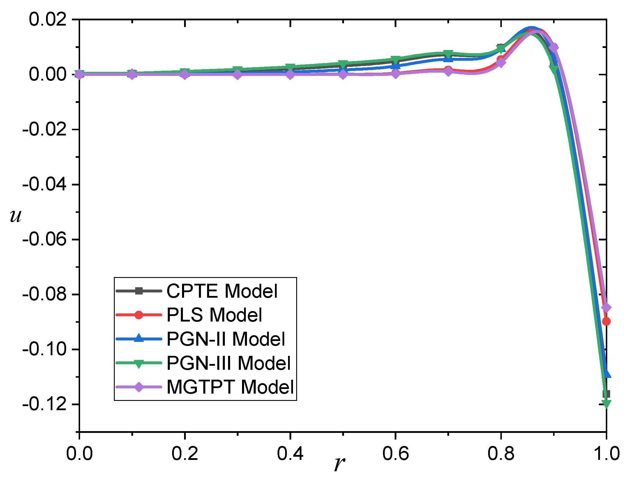
The different models for the distribution of displacement $u$ across radius $r$ are compared in Figure 2 and Table 2. The numerical data and graphs show that the displacement $u$ starts with negative values, then rapidly increases until it reaches its maximum positive value, then gradually fades to zero. It can also be seen that the displacement curves converge in the case of all the different models, despite the different values. Thus, it can be concluded that the effect of thermal parameters is weak on the displacement distributions.

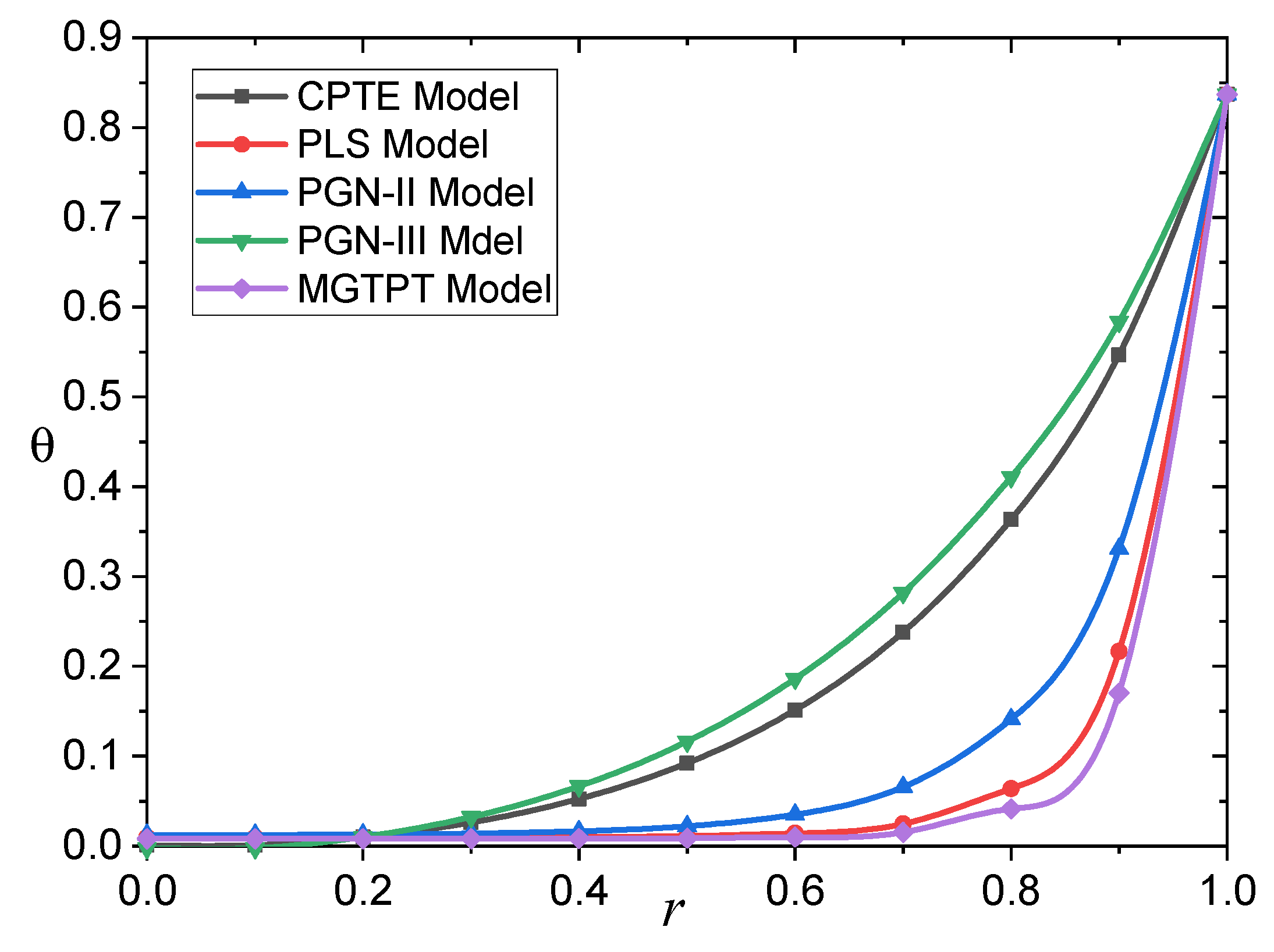
The five curves predicted by various photo-thermoelasticity models with and without thermal parameters for the carrier density $N$ against the radial distance $r$ are shown in Figure 3 and Table 3. Due to the recombination of charge carriers, the carrier density peaks at the surface of the sphere $r=1$ and progressively falls as the radial distance increases until it approaches the steady state. The results in the case of the GN-III model are characterized by a larger carrier density $N$ than the MGTPT, with a similar behavior to the PLS and PGN-II models.

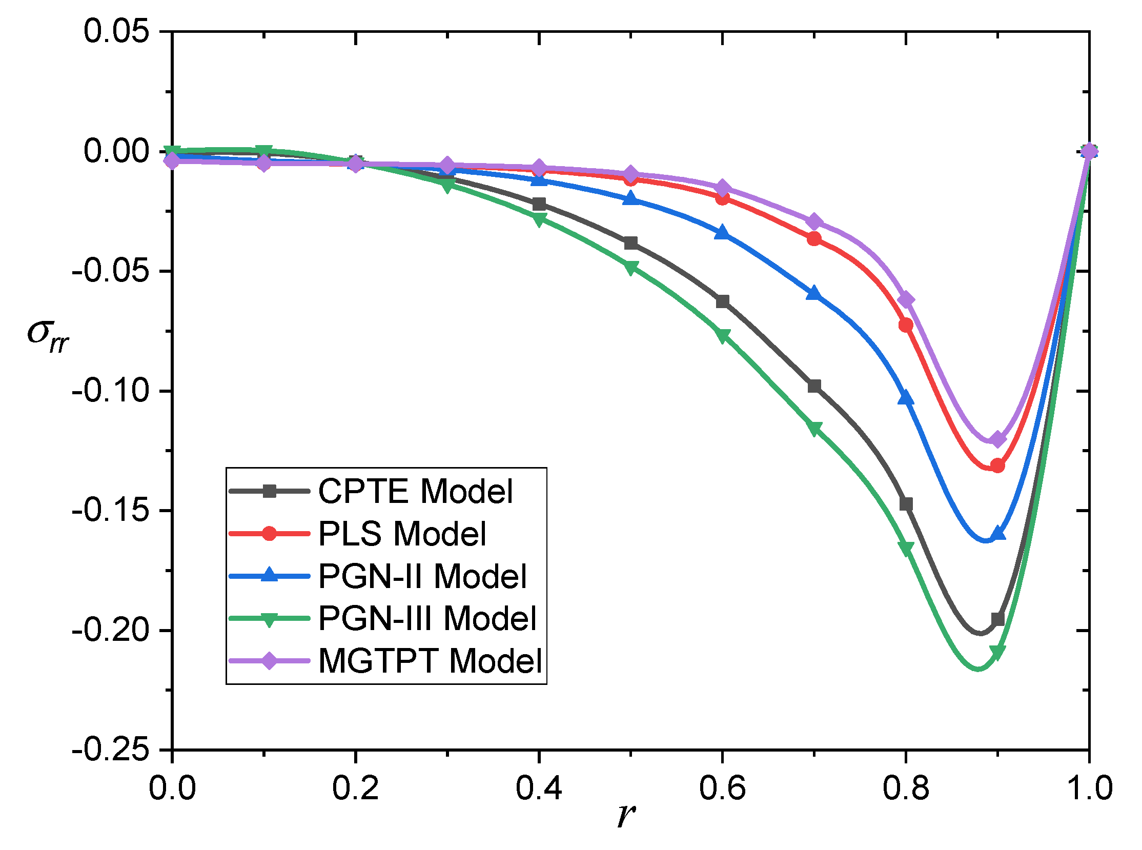
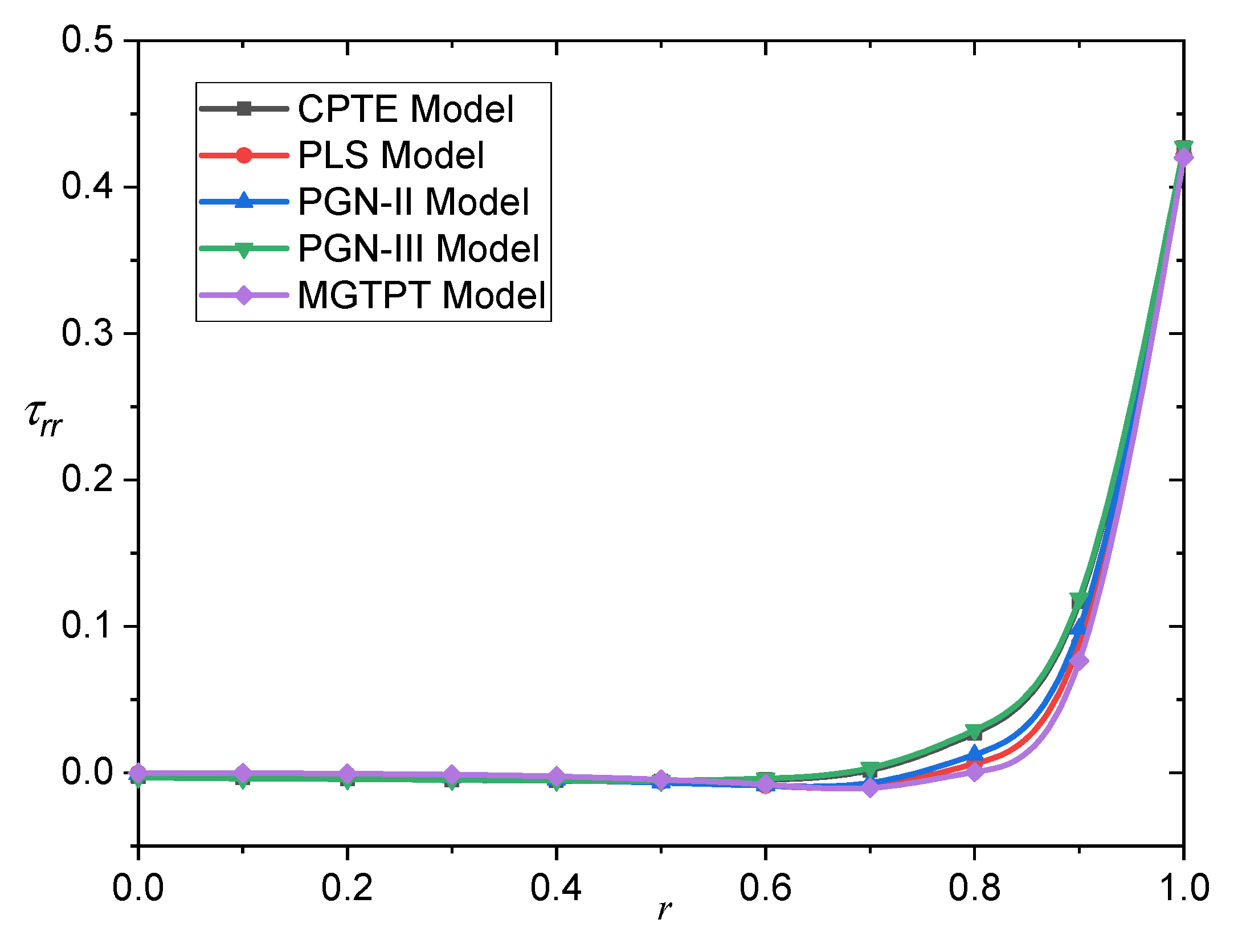
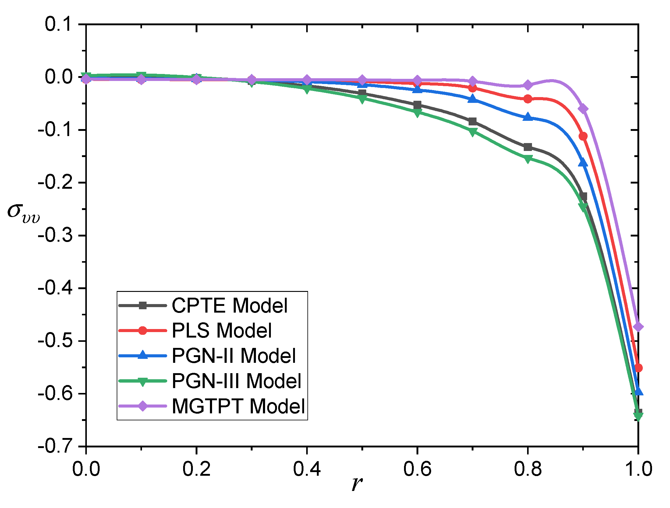
The fluctuation of the radial stress ${\sigma }_{rr}$ with respect to the distance for different models is illustrated in Figure 4 and Table 4. It should be noted that the pressure always starts from zero to respect the boundary requirements, and then gradually decreases until it reaches the lower value at a certain position near the surface of the sphere, and then gradually increases to zero. Figure 5 and Table 5 illustrate the fluctuation of hoop stress ${\sigma }_{\vartheta \vartheta }$ versus $r$ for several models of photo-thermoelasticity. In all cases, the hoop stress is initially negative and progressively reduces until it reaches zero. The stresses emphasize the location of the medium next to the spherical surface with time, which is consistent with the data in [44]. In addition, when the radial width increases, the value and amplitude of fields measured at the surface increase. Because of this, ref. [45] provides reasons for this phenomenon.

Figure 6 and Table 6 demonstrate the Maxwell’s stress ${\tau }_{rr}$ fluctuation vs. $r$ over a wide range of $0<r\le 1$ for different models of photo-thermoelasticity. The speed of propagation of electromagnetic waves is limited and corresponds to the physical behavior of photo-thermal materials. We also note that the behavior of the curves is the same and that there are small differences between the different models.

5.2. The Influence of Angular Velocity of Rotation

The analysis of the propagation of plane photo-thermoelastic waves in a spinning solid appears to have received little attention. Because most large bodies have an angular motion, such as the earth, moon, and other planets, studying the propagation of planar thermoelastic or magneto-photo-thermoelastic waves in a rotating medium with thermal relaxation appears to be more realistic.

Table 7. The variation of different photothermal fields with different rotation parameter Ω.

$\mathit{r} \mathbf{=} \mathbf{0.9}\mathbf{.}$	$\mathbf{\Omega }$	$\mathit{\theta }$	$\mathit{u}$	$\mathit{N}$	${\mathit{\sigma }}_{\mathit{r}\mathit{r}}$	${\mathit{\sigma }}_{\mathit{z}\mathit{z}}$	${\mathit{\tau }}_{\mathit{r}\mathit{r}}$
CPTE	0	0.579961	0.00301477	0.002452210	−0.207303	−0.233091	0.1199820
	5	0.504634	0.00357827	0.001947390	−0.181736	−0.202836	0.1086730
	10	0.432417	0.00393590	0.000754857	−0.157142	−0.173095	0.0969131
PLS	0	0.380552	0.00839796	−0.03440070	−0.137101	−0.117767	0.1044720
	5	0.329505	0.00822557	−0.02989960	−0.120069	−0.102062	0.0947231
	10	0.280648	0.00789131	−0.02610120	−0.103682	−0.086496	0.0845178
PGN-II	0	0.439059	0.00712821	−0.02102290	−0.157300	−0.154178	0.1099490
	5	0.380777	0.00714752	−0.01877670	−0.137766	−0.133374	0.0996657
	10	0.324984	0.00699024	−0.01693120	−0.118985	−0.113127	0.0889246
PGN-III	0	0.621530	0.00156896	0.01446110	−0.222413	−0.261453	0.1222750
	5	0.541439	0.00230369	0.01131410	−0.195131	−0.226684	0.1107220
	10	0.464567	0.00282672	0.00831416	−0.168858	−0.193305	0.0987226
MGTPT	0	0.344723	0.00902147	−0.0437438	−0.124892	−0.094312	0.100625
	5	0.298095	0.00874568	−0.0375427	−0.109368	−0.082045	0.0912424
	10	0.253494	0.00831745	−0.0323135	−0.0944313	−0.069583	0.0814059

explains the variations of different photothermal fields with different rotation parameter $\mathsf{\Omega }$ under different photo-thermoelastic models (CPTE, PLS, PGN-II, PGN-III, and MGTPT). The numerical results were calculated at a single value of the distance $r$, which is $r=0.9$. In the case of all the different models, it was found that the differences in the magnitudes in all the studied fields decreased with the increase in the angular velocity, except for the displacement. We note that the displacement distribution decreases with the angular velocity in the case of the PLS, PGN-II, and MGTPT models, while it increases in the case of the CPTE and PGN-III models.

In this section, we explore the response of distinct photothermal fields as the rotation parameter $\mathsf{\Omega }$ changes only in the case of the generalized elastic photothermal model (MGTPT). For comparative purposes, we will choose three numbers for the amount of rotational speed $\mathsf{\Omega }$. The rotating example is chosen with $\mathsf{\Omega }=5, 10$, while the nonrotating case is chosen with $\mathsf{\Omega }=0$. Figure 7, Figure 8, Figure 9, Figure 10, Figure 11 and Figure 12 illustrate the distribution of the data for the various fields studied.

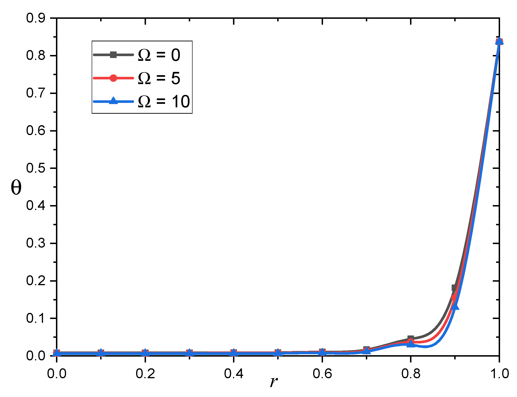
As seen in Figure 7, Figure 8 and Figure 12, the parameter $\mathsf{\Omega }$ has a relatively little influence on temperature $\theta$, displacement $u$, and Maxwell’s stress ${\tau }_{rr}$. This phenomenon is consistent with the results reported in the references [44,45]. We can also see in Figure 7, Figure 8 and Figure 12 that as the rotation parameter $\mathsf{\Omega }$ increases, the field variables $\theta$, $u$, and ${\tau }_{rr}$ decrease. 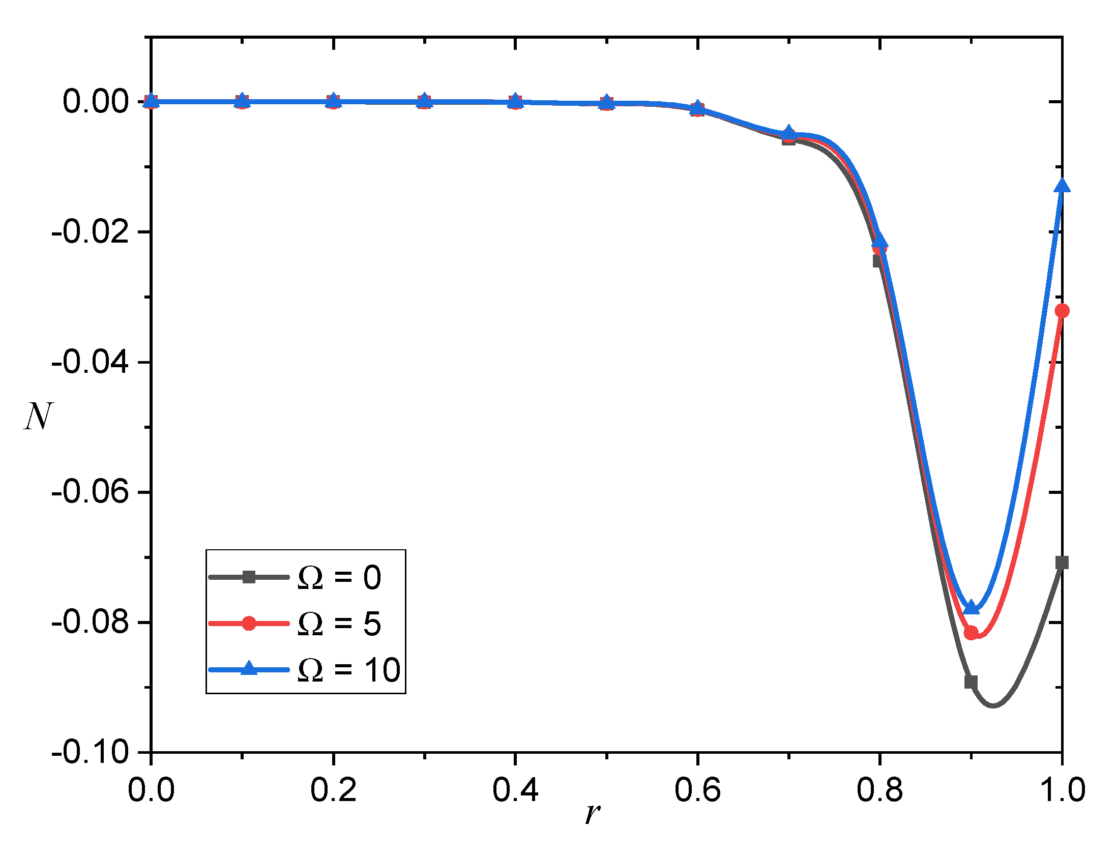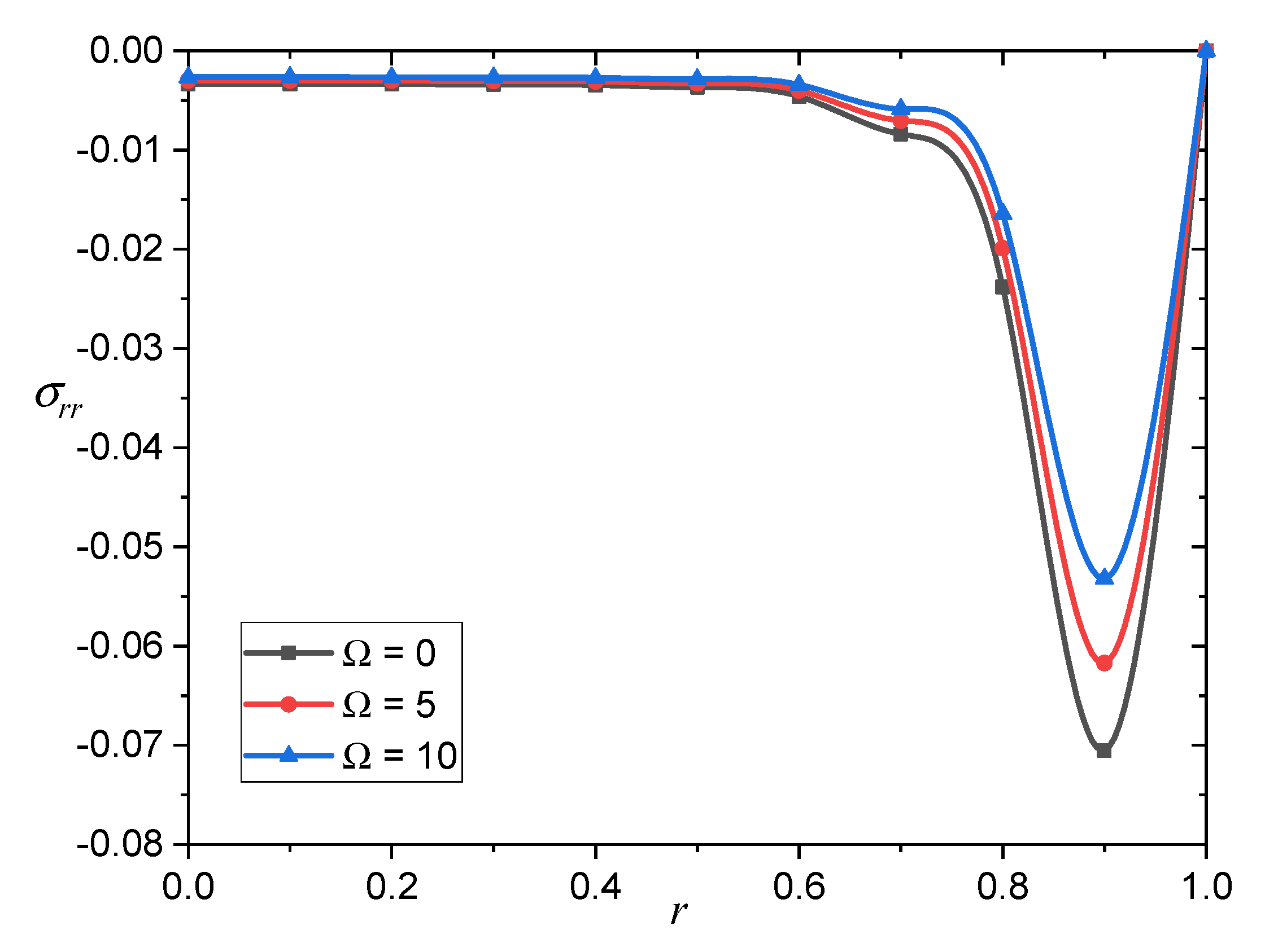Furthermore, as shown in Figure 9, Figure 10 and Figure 11, the rotational parameter $\mathsf{\Omega }$ has a great influence on the carrier density $N$ and the thermal stresses ${\sigma }_{rr}$ and ${\sigma }_{\vartheta \vartheta }$.

Figure 10 illustrates that increasing the amount of $N$ increases the carrier density numerical values. Figure 10 shows the change in thermal stress ${\sigma }_{rr}$ as a function of radius $r$ and parameter $\mathsf{\Omega }$. We can see that the rotational parameter $\mathsf{\Omega }$ has a significant impact on the radial stress profile ${\sigma }_{rr}$. As the parameter $\mathsf{\Omega }$ is increased, the stress ${\sigma }_{rr}$ increases. Furthermore, the amplitude of the stress ${\sigma }_{\vartheta \vartheta }$ distribution increases as $\mathsf{\Omega }$ increases.

6. Conclusions

A novel photo-thermoelastic model, including the Moore–Gibson–Thompson equation, is presented in this paper. The type III Green–Naghdi model, as well as the Lord and Shulman equations, are all included in the improved photothermal model. The interplay of heat, plasma, and elastic waves in semiconductor materials is explored in this expanded model, which is significant. Furthermore, unlike traditional models, this model permits heat-elastic optical waves to propagate at restricted speeds. So far, only a few articles on our topic have been written in the scientific literature. As special instances of the suggested model, several thermoelastic and photothermal models may be constructed.

From the quantitative data, we may conclude that the thermal relaxation time reduces the mechanical and thermo-optical waves along the axes. It is also noted that the behavior of waves in different physical fields depends on the speed of rotation of the medium. The new photo-thermoelasticity model allows heat to go through a medium at a finite velocity rather than an infinity-speed wave as in the case of the CPTE model. Compared to the PGN-III model, the extended MGTPT model more accurately describes the photo-thermoelastic process. In contrast to previous generalized thermoelasticity models, the PGN-III model’s results show convergence with the conventional elasticity model (CPTE), which does not disappear quickly within the body.

Scientists working in fields, such as physics, material design, thermal efficiency, and geophysics will benefit greatly from the information presented in this study. The approach employed in this investigation can be used to address a variety of thermodynamic challenges.