Determining Number of Factors in Dynamic Factor Models Contributing to GDP Nowcasting

Abstract

Real-time nowcasting is a process to assess current-quarter GDP from timely released economic and financial series before the figure is disseminated in order to catch the overall macroeconomic conditions in real time. In economic data nowcasting, dynamic factor models (DFMs) are widely used due to their abilities to bridge information with different frequencies and to achieve dimension reduction. However, most of the research using DFMs assumes a fixed known number of factors contributing to GDP nowcasting. In this paper, we propose a Bayesian approach with the horseshoe shrinkage prior to determine the number of factors that have nowcasting power in GDP and to accurately estimate model parameters and latent factors simultaneously. The horseshoe prior is a powerful shrinkage prior in that it can shrink unimportant signals to 0 while keeping important ones remaining large and practically unshrunk. The validity of the method is demonstrated through simulation studies and an empirical study of nowcasting U.S. quarterly GDP growth rates using monthly data series in the U.S. market.

1. Introduction

Real-time nowcasting is a process to assess current-quarter GDP from timely released economic and financial series before the figure is disseminated in order to catch the overall macroeconomic conditions in real time. This is of interest because most data are released with a lag and are released subsequently. In theory, any release, no matter at what frequency, may affect current-quarter estimates and their precision potentially. Both forecasting and nowcasting are important tasks for central banks for policy decision-making; for example, monetary policies need to be made in real time and are based on assessments of current and future economic conditions. Additionally, estimated current-quarter GDP figures are often used as relevant inputs for model-based longer-term forecasting exercises in banks.

Real-time nowcasting faces some difficulties. The first one is how to bridge monthly data series with the quarterly GDP. Bafigi et al. [1], Rünstler and Sédillot [2], and Kitchen and Monaco [3] studied the idea of bridge equations which use small models to “bridge” the information contained in one or a few key monthly data with the quarterly growth rate of GDP. However, they involve judgmental nowcasts and only deal with a few monthly data series. The second difficulty is how to deal with a large number of monthly data series. For macroeconomic forecasting, factor models (FMs) are widely used at central banks and other institutions to achieve dimension reduction. Many authors, such as Boivin and Ng [4], Forni et al. [5], and D’Agostino and Giannone [6], have shown that these models are successful in this regard. However, they did not use FMs specifically for the problem of real-time nowcasting. There are other existing approaches to tackle the high dimensional issue. One example is Eraslan and Schröder [7] who dealt with this over-parameterized issue in GDP nowcasting by implementing the dynamic model averaging method (Raftery et al. [8]). However, they did not talk about how to handle the unbalanced structure of the data caused by different release dates with different lags in each month. Moreover, they assumed a fixed number of factors, while in our paper the focus is to determine the number of factors contributing to GDP nowcasting. The third challenge is that a large number of monthly data series are released with different lags, causing unbalanced data at the end of the sample. Some authors, including Croushore and Stark [9], Koenig et al. [10] and Orphanides [11], discussed about this issue, but they are not focusing on the statistical estimation.

Giannone et al. [12] provided a frequentist inference framework for the parametric dynamic factor models (DFMs). In their framework, they took advantage of different data releases throughout the month and updated the nowcast based on each new data release. The authors combined the idea of connecting monthly series with the nowcast of quarterly GDP and the idea of using data with different releases within a single statistical framework. Their model combines principal component analysis (PCA) with modified Kalman Filter (KF) to deal with the unbalanced feature of the data. Hereafter, we call the method proposed in Giannone et al. the GRS approach.

In this paper, we borrow the idea of DFMs from Giannone et al. [12] and propose a Bayesian Monte Carlo Markov Chain (MCMC) approach to deal with the real-time nowcasting problem. For DFMs, one important aspect is to determine the number of factors. In the GRS approach, the number of factors is assumed to be fixed, which is determined by looking at the cumulative proportions of variances explained by the first few principle components from PCA, and the same set of factors is assumed to have prediction power on GDP. Bai and Ng [13] showed that the number of factors could be estimated consistently in a large panel of data setting. In this paper, we impose a cap on the number of factors in the DFM structure but allow an unknown number of factors to contribute to GDP prediction. We propose to apply the horseshoe shrinkage (Carvalho et al. [14,15]) on the coefficients of factors in the prediction equation. One big advantage of the horseshoe shrinkage over other traditional shrinkages is that it can shrink unimportant signals to 0 while keeping important ones large and practically unshrunk (more details will be discussed in Section 2). After estimation, any coefficient that is shrunk to 0 indicates its corresponding factor has no prediction power. As a result, the number of coefficients that remain large after strong shrinkage is a good estimate of an unknown number of factors with prediction power on GDP. Our Bayesian MCMC approach can also provide a more natural way to deal with the unbalanced data structure due to real-time data releasing and estimate all parameters, including the number of contributing factors and latent dynamic factors in a single framework. We refer to this Bayesian approach as the BAY approach. Through simulation studies, we evaluate the abilities of our BAY approach in estimating an unknown number of contributing factors and in producing reliable nowcasts in real time. The validity of the BAY approach is also examined by applying it to nowcast U.S. quarterly GDP growth rates.

The rest of this paper is organized as follows. Section 2 sets up the model structure, introduces the horseshoe shrinkage into our model, and stylizes the data structure. In Section 3, we introduce the Bayesian MCMC estimation method with nowcasting equations. In Section 4, we conduct simulation studies. In Section 5, an empirical study of nowcasting U.S. GDP growth rates is presented. Section 6 concludes the paper. A list of abbreviations used in this paper is provided in Abbreviations.

2. Model Set-Ups, Horseshoe Shrinkage, and Data Structure

In Section 2.1, the model set-ups used in the BAY approach are illustrated. In Section 2.2, we introduce the horseshoe shrinkage idea and how to implement it in our BAY approach to estimate number of contributing factors. In Section 2.3, we formalize the unbalanced data structure.

2.1. Dynamic Factor Models

In this section, we introduce the Dynamic Factor Model structure and how it can reduce dimension and bridge our monthly released series with quarterly released GDP.

Since the number of monthly series is vast, modeling GDP on all available series can involve too many parameters; hence, the model would perform poorly in forecasting because of large uncertainty in the parameters’ estimation. The fundamental idea of Giannone et al. [12] is to use DFMs to exploit the collinearity of the series by summarizing all the available information into a few common latent factors. Due to collinearity, a linear combination of the common factors is able to capture the dynamic interaction among the series and to provide a model that only requires a limited number of parameters and thus works well in forecasting. In this paper, our DFM is specified in the following ways.

First, assume that the monthly series are linear functions of a few unobserved common factors ${\mathbf{F}}_t$,

$${\mathbf{x}}_t=\mathbf{\mu }+\mathbf{\Theta }{\mathbf{F}}_t+{\epsilon }_t,$$

(1)

where ${\mathbf{x}}_t={(x_{1,t},\cdots ,x_{n,t})}^{\prime }$ is the $n\times 1$ monthly series vector at month t, for $t=1,2,\dots ,T$, ${\mathbf{F}}_t={(f_{1t},\cdots ,f_{rt})}^{\prime }$ is the $r\times 1$ common factor vector at month t, r is the number of latent factors ($r<<n$) which is usually assumed to be known and fixed, $\mathbf{\Theta }$ is the $n\times r$ factor loading, $\mathbf{\mu }$ is the $n\times 1$ mean vector, and the $n\times 1$ error vector ${\mathit{\epsilon }}_t\sim N(\mathbf{0},{\mathbf{\Omega }}_{n\times n})$. Note that the difference between Equation (1) and regular multiple regression is that the factors ${\mathbf{F}}_t$ are unobserved latent variables, while the predictors in multiple regression are observed. The latent factors ${\mathbf{F}}_t$ serve an important role of bridging information from monthly series to quarterly GDP.

Then, we further specify the dynamic of the common factors as a vector auto-regression:

$${\mathbf{F}}_t=\mathbf{A}{\mathbf{F}}_{t-1}+{\mathbf{u}}_t,$$

(2)

where $\mathbf{A}=diag(a_1,a_2,\dots ,a_r)$ and ${\mathbf{u}}_t\sim N(\mathsf{0},{\mathbf{\Sigma }}_{r\times r})$ with $\mathbf{\Sigma }=diag({\sigma }_1^2,{\sigma }_2^2,\dots ,{\sigma }_r^2)$. It is known that factor dynamic models can suffer from non-identifiable issues. Following Stock and Watson [16], we construct two sets of restrictions: $|a_j|<1$ and $\frac{{\sigma }_i^2}{(1-a_i^2)}<\frac{{\sigma }_j^2}{(1-a_j^2)}$ for $1\le i<j\le r$. These restrictions together with the prior distribution of $\mathbf{\Theta }$ (specified later) satisfy the identification assumptions in Stock and Watson [16], and can identify factors up to a change of sign.

Finally, we assume that the nowcast of the GDP at quarter k is a linear function of the common factors at each month in the current quarter and the GDP from the previous quarter:

$$y_k={\beta }_0+{\mathbf{\beta }}_1^{\prime }{\mathbf{F}}_{3k}+{\mathbf{\beta }}_2^{\prime }{\mathbf{F}}_{3k-1}+{\mathbf{\beta }}_3^{\prime }{\mathbf{F}}_{3k-2}+{\beta }_4{y}_{k-1}+{\nu }_k,$$

(3)

where ${\beta }_0$ and ${\beta }_4$ are scalars, ${\mathbf{\beta }}_i={({\beta }_{i1},\dots ,{\beta }_{ir})}^{\prime }$, $i=1,2,3$, are $r\times 1$ vectors and ${\nu }_k\sim N(0,{\eta }^2)$ for $k=1,\dots ,K$. Here, the number T (the end of monthly series) and the number K (the end of quarterly GDP series) satisfy $3K+1\le T\le 3K+3$. The DFMs specified this way can successfully bridge quarterly released GDP with monthly financial or economic series and achieve dimension reduction.

2.2. Horseshoe Shrinkage

In this section, the horseshoe shrinkage idea is introduced, and we discuss how it can be implemented in our model framework to estimate the number of contributing factors.

In Carvalho et al. [14], the horseshoe prior was first introduced as a shrinkage prior. Follett and Yu [17] shown that the horseshoe prior competes favorably with shrinkage schemes commonly used in Bayesian multivariate regression models. To illustrate the idea, let us first consider a simple mean model $z_j\stackrel{ind}{\sim }N({\mu }_j,{\sigma }^2)$ for $j=1,\dots ,R$. We assume $\mathbf{\mu }=({\mu }_1,\dots ,{\mu }_R)$ is sparse and some ${\mu }_j$ might be equal to 0. We can assign the horseshoe prior to ${\mu }_j$ for $j=1,\dots ,R$ by letting ${\mu }_j|{\lambda }_j,\tau \stackrel{ind}{\sim }N(0,{\lambda }_j^2{\tau }^2)$ with ${\lambda }_j\stackrel{iid}{\sim }HalfCauchy(0,1)$. Here, $\tau$ is referred to as the global shrinkage prior and ${\lambda }_j$ is referred to as the local shrinkage prior. Figure 1 plots the densities for the horseshoe (setting $\tau =1$ for simplicity), Laplacian, and Student-t priors, respectively. As shown in Figure 1, compared to Laplacian or Student-t priors, the horseshoe has flat tails which allow strong signals that remain un-shrunk. It also has an “infinitely” tall spike at the center which can provide severe shrinkage for elements near zero. This feature makes the horseshoe prior a very useful shrinkage prior.

Figure 1. Densities of the implied prior on ${\mu }_j$ based on the horseshoe prior, the t prior, and the Laplacian prior.

Furthermore, it was showed in Carvalho et al. [14] that, for $\tau ={\sigma }^2=1$,

$$E\left({\mu }_j\right|z_1,\dots ,z_R,{\lambda }_j)=(1-{\kappa }_j)z_j+{\kappa }_{j}0=(1-{\kappa }_j)z_j,$$

where ${\kappa }_j=\frac{1}{1+{\lambda }_j^2}$. When ${\kappa }_j=0$, $E\left({\mu }_j\right|z_1,\dots ,z_R,{\lambda }_j)=z_j$, it indicates that the signal from data dominates; when ${\kappa }_j=1$, $E\left({\mu }_j\right|z_1,\dots ,z_R,{\lambda }_j)=0$, it means that ${\mu }_j$ is shrunk to 0. Thus, ${\kappa }_j$ is referred to as the Shrinkage Profile which measures the shrinkage level:

$${\kappa }_j=\left\{\begin{array}{cc}0\hfill & \mathrm{little}\mathrm{shrinkage}\left(\mathrm{Important}\right)\hfill \\ 1\hfill & \mathrm{extreme}\mathrm{shrinkage}(\mathrm{Not}\mathrm{important}).\hfill \end{array}\right.$$

(4)

The Half Cauchy prior on ${\lambda }_j$ implies a $Beta(0.5,0.5)$ prior on the Shrinkage Profile ${\kappa }_j$. Figure 2 shows the implied prior on ${\kappa }_j$ for the horseshoe prior, the student’s t prior, and the Laplacian prior. As shown in the figure, unlike the Laplacian prior and t prior, the density of ${\kappa }_j$ implied by the horseshoe prior is unbounded at both 0 and 1 with a small mass in between (a horseshoe shape). Being unbounded at 0 allows effects to grow large (little shrinkage) while being unbounded at 1 can shrink effects until they are fully removed from the equation.

Figure 2. Densities of the shrinkage profile ${\kappa }_j$ based on the horseshoe prior, the t prior, and the Laplacian prior. ${\kappa }_j=0$ means no shrinkage and ${\kappa }_j=1$ means total shrinkage.

We apply this horseshoe shrinkage idea to the prediction Equation (3) as follows:

$$y_k={\beta }_0+{\mathbf{\beta }}_1^{\prime }\mathbf{S}{\mathbf{F}}_{3k}+{\mathbf{\beta }}_2^{\prime }\mathbf{S}{\mathbf{F}}_{3k-1}+{\mathbf{\beta }}_3^{\prime }\mathbf{S}{\mathbf{F}}_{3k-2}+{\beta }_4{y}_{k-1}+{\nu }_k,$$

(5)

where $\mathit{S}=diag(\tau {\lambda }_1,\dots ,\tau {\lambda }_R)$, and R is the largest possible number of latent factors. The cap R is predetermined, satisfying $r<R<<n$. Now, ${\mathbf{\beta }}_i={({\beta }_{i1},\dots ,{\beta }_{iR})}^{\prime }$, $i=1,2,3$, are $R\times 1$ vectors, ${\mathbf{F}}_t={(f_{1t},\cdots ,f_{Rt})}^{\prime }$ are $R\times 1$ common factors at month t, and dimensions for $\mathbf{A}$, $\mathbf{\Sigma }$, and $\mathbf{\Theta }$ are changed accordingly.

In this specification, $\tau$ is the global shrinkage prior and ${\lambda }_j$ ($j=1,\dots ,R$ ) are local shrinkage priors. We set ${\lambda }_j\sim HalfCauchy(0,{\nu }_{\lambda }^j)$, where $0<{\nu }_{\lambda }<1$. In this way, we assume that the importance of factors decreases when j goes from 1 to R. If we put priors ${\beta }_{ij}\stackrel{iid}{\sim }N(0,1)$, $i=1,2,3$, $j=1,\dots ,R$ and define ${\tilde{\beta }}_{ij}:=\tau {\lambda }_j{\beta }_{ij}$, then ${\tilde{\beta }}_{ij}|\tau ,{\lambda }_j\stackrel{ind}{\sim }N(0,{\tau }^2{\lambda }_j^2)$, and Equation (5) changes to be

$$y_k={\beta }_0+\sum _{j=1}^R{\tilde{\beta }}_{1j}{f}_{3k,j}+\sum _{j=1}^R{\tilde{\beta }}_{2j}{f}_{3k-1,j}+\sum _{j=1}^R{\tilde{\beta }}_{3j}{f}_{3k-2,j}+{\beta }_4{y}_{k-1}+{\nu }_k.$$

(6)

It can be seen that ${\tilde{\mathit{\beta }}}_{.j}={({\tilde{\beta }}_{1j},{\tilde{\beta }}_{2j},{\tilde{\beta }}_{3j})}^{\prime }$ is the coefficient connecting factor j to GDP in the prediction equation. By such a specification, we successfully impose the horseshoe shrinkage prior on the coefficients ${\tilde{\mathit{\beta }}}_{.j}$’s. The magnitudes of the estimated profiles, ${\kappa }_j=\frac{1}{1+{\lambda }_j}$ (for $j=1,\dots ,R$), give us some information about which ${\tilde{\mathbf{\beta }}}_{.j}$ should be shrunk to 0 and which should not. If ${\kappa }_j$ is close to 1, indicating extremely strong shrinkage on ${\tilde{\mathit{\beta }}}_{.j}$, factor j then has no prediction power on GDP. As a consequence, the number of remaining un-shrunk ${\tilde{\mathit{\beta }}}_{.j}$ determines the number of contributing factors.

2.3. The Unbalanced Structure of the Data

In this section, we provide descriptions of the unbalanced data structure and notations used to represent the unbalanced structure.

In real time, macroeconomic series are released with diverse lags. At a particular release date, some series have observations up through the current month, whereas for others, the most recent observations maybe come from previous months. Dealing with these kinds of unbalanced data is vital for nowcasting.

Let ${\mathit{x}}_T=(x_{1,T},\dots ,x_{n,T})$ be the $n\times 1$ vector denoting n monthly data series at month T (the end of the sample), and $y_K$ be quarterly GDP at quarter K. Assume there are Q different release dates at each month. Each release date is denoted as $(q,T)$, representing the qth release date in month T, where $q=1,\dots ,Q$. New series are released on each release date. Since some series for the current month may be released in the future, let $T_q$ denote the latest month in which the data are balanced. For $t=T_q+1,\dots ,T$, the releasing set $v_{q,t}$ collects indexes of all $x_{i,t}^{\prime }$s that have been released at or before the release date $(q,T)$, and this set of available series is denoted as ${\mathbf{x}}_{i\in v_{q,t}}$. Without loss of generality, for each month, we assume the release dates for all series are fixed.

Table 1 gives a simple example of the data set available for nowcasting. In this example, there are $n=6$ monthly series, ${\mathbf{x}}_t=(x_{1,t},\dots ,x_{6,t})$, released at three (i.e., $Q=3$) releasing dates. For month T, cells with gray color represent series that are available before T. Suppose $(x_{5,T-2},x_{6,T-2})$ are released at the first releasing date $(1,T)$, $(x_{3,T-1},x_{4,T-1})$ are released at the second releasing date $(2,T)$, and $(x_{1,T},x_{2,T})$ are released at the third releasing date $(3,T)$. Thus, for the third releasing date $(3,T)$, $T_q=T-2$, $v_{3,T-1}=\{1,2,3,4\}$, ${\mathbf{x}}_{i\in v_{3,T-1}}=(x_{1,T-1},x_{2,T-1},x_{3,T-1},x_{4,T-1})$, and $v_{3,T}=\{1,2\}$, ${\mathbf{x}}_{i\in v_{3,T}}=(x_{1,T},x_{2,T})$. If we want to nowcast GDP in the current quarter $y_{K+1}$ at the first release date in the second month of the quarter, so here $T=3K+2$. The series available to use at the release date $(1,T)$ are highlighted in gray and orange color, i.e., $\{{\mathbf{x}}_1,\cdots ,{\mathbf{x}}_{T-2},{\mathbf{x}}_{i\in v_{1,T-1}}\}$. The series available to use at the release date $(2,T)$ are highlighted in gray, orange, and green, i.e., $\{{\mathbf{x}}_1,\cdots ,{\mathbf{x}}_{T-2},{\mathbf{x}}_{i\in v_{2,T-1}}\}$.

Table 1. An example of the overall releasing pattern. Gray colored cells represent available series before T. Orange, green, and blue represent the 1st, 2nd, and 3rd release within T, respectively.

k	1			…	K			K + 1
t	1	2	3	…	T − 4	T − 3	T − 2	T − 1	T	T + 1
${\mathbf{x}}_{i,t}$	$x_{1,1}$	$x_{1,2}$	$x_{1,3}$	…	$x_{1,T-4}$	$x_{1,T-3}$	$x_{1,T-2}$	$x_{1,T-1}$	$x_{1,T}$	NA
	$x_{2,1}$	$x_{2,2}$	$x_{2,3}$	…	$x_{2,T-4}$	$x_{2,T-3}$	$x_{2,T-2}$	$x_{2,T-1}$	$x_{2,T}$	NA
	$x_{3,1}$	$x_{3,2}$	$x_{3,3}$	…	$x_{3,T-4}$	$x_{3,T-3}$	$x_{3,T-2}$	$x_{3,T-1}$	NA	NA
	$x_{4,1}$	$x_{4,2}$	$x_{4,3}$	…	$x_{4,T-4}$	$x_{4,T-3}$	$x_{4,T-2}$	$x_{4,T-1}$	NA	NA
	$x_{5,1}$	$x_{5,2}$	$x_{5,3}$	…	$x_{5,T-4}$	$x_{5,T-3}$	$x_{5,T-2}$	NA	NA	NA
	$x_{6,1}$	$x_{6,2}$	$x_{6,3}$	…	$x_{6,T-4}$	$x_{6,T-3}$	$x_{6,T-2}$	NA	NA	NA
$y_k$	$y_1$			…	$y_K$			$y_{K+1}$

The goal is to nowcast $y_{K+1}$ with all available information including ${\mathit{x}}_t$ series and $y_k$ series at each releasing date $(q,T)$ in month T. Here, $T=3K+1,3K+2,3K+3$, indicating the first month, second month, and third month nowcast. At every new release date $(q,T)$, model parameters are updated with new information added from the new released series, and nowcast of $y_{K+1}$ is re-produced. How to deal with this unbalanced data in our BAY approach will be discussed in details in Section 3.

3. Estimation Method and Nowcasting

In Section 3.1, we introduce the Bayesian MCMC algorithm to estimate model parameters and latent factors and to determine the number of contributing factors. In Section 3.2, nowcasting formulas are provided.

3.1. Estimating Dynamic Factor Models Using Bayesian MCMC

In this section, we first introduce our method of implementing the unbalanced data into our model framework naturally. Then, we finish our model specification by assigning priors in Bayesian Framework. Finally, the MCMC procedure is discussed in detail.

As discussed in Section 2, macroeconomic series are released with diverse lags in real time. Thus, a difficulty in real-time nowcasting is to deal with unbalanced data. In this section, we develop a computational Bayesian MCMC approach that can tackle this issue naturally.

To deal with the missing data in ${\mathbf{x}}_{i\in v_{q,t}}$ at the end of the sample, we introduce the $n_q\times n$ indicator matrix ${\mathbf{1}}_{v_{q,t}}$ by deleting the ith row from the identity matrix ${\mathbf{1}}_{n\times n}$ if $i\notin v_{q,t}$. For the example discussed in Section 2, at the third releasing date $(3,T)$ in month T, $v_{3,T-1}=\{1,2,3,4\}$. Therefore, removing the fifth and sixth row of ${\mathbf{1}}_{6\times 6}$ gives us

$${\mathbf{1}}_{v_{3,T-1}}=\left(\begin{array}{cccccc}1& 0& 0& 0& 0& 0\\ 0& 1& 0& 0& 0& 0\\ 0& 0& 1& 0& 0& 0\\ 0& 0& 1& 0& 0& 0\end{array}\right).$$

Similarly, for the index set $v_{3,T}=\{1,2\}$, deleting the last four rows of ${\mathbf{1}}_{6\times 6}$ leads to

$${\mathbf{1}}_{v_{3,T}}=\left(\begin{array}{cccccc}1& 0& 0& 0& 0& 0\\ 0& 1& 0& 0& 0& 0\end{array}\right).$$

Then, we can simply rewrite ${\mathbf{x}}_{i\in v_{q,t}}$ as ${\mathbf{x}}_{i\in v_{q,t}}={\mathbf{1}}_{v_{q,t}}{\mathbf{x}}_t.$

To better derive the posterior distributions, we express the dynamic of ${\mathbf{x}}_t$ in Equation (1) as:

$${\mathbf{x}}_t=\mathbf{\mu }+[{\mathit{I}}_{n\times n}\otimes {\mathbf{F}}_t^{\prime }]\ast \mathbf{\theta }+{\mathbf{\epsilon }}_t,$$

where $\mathbf{\theta }=vec\left(\mathbf{\Theta }\right)={({\theta }_1,\dots ,{\theta }_n)}^{\prime }$, ${\theta }_i$ is a $1\times R$ vector representing the ith row of $\mathbf{\Theta }$, $i=1,2,\dots ,n$, and the symbol ⊗ denotes the Kronecker product. Thus, for the qth releasing date in month T, the conditional density for ${\mathbf{x}}_t$ is

$$\left\{\begin{array}{cc}{\mathbf{x}}_t|{\mathbf{F}}_t,\mathbf{\Theta },\mathbf{\Omega }\sim N(\mathbf{\mu }+[{\mathit{I}}_{n\times n}\otimes {\mathbf{F}}_t^{\prime }]\ast \mathbf{\theta },\mathbf{\Omega })\hfill & \mathrm{for}t=1,\dots ,T_q\hfill \\ {\mathbf{1}}_{v_{q,t}}{\mathbf{x}}_t|{\mathbf{F}}_t,\mathbf{\Theta },\mathbf{\Omega }\sim N({\mathbf{1}}_{v_{q,t}}(\mathbf{\mu }+[{\mathit{I}}_{n\times n}\otimes {\mathbf{F}}_t^{\prime }]\ast \mathbf{\theta }),{\mathbf{1}}_{v_{q,t}}\mathbf{\Omega }{\mathbf{1}}_{v_{q,t}}^{\prime })\hfill & \mathrm{for}t=T_q+1,\dots ,T,\hfill \end{array}\right.$$

(7)

the conditional density of ${\mathbf{F}}_t$ is

$${\mathbf{F}}_t|{\mathbf{F}}_{t-1},\mathbf{A},\mathbf{\Sigma }\sim N(\mathbf{A}{\mathbf{F}}_{t-1},\mathbf{\Sigma }),fort=2,\dots ,T,$$

(8)

and the conditional density of $y_k$ is

$$y_k|{\mathbf{F}}_{3k},{\mathbf{F}}_{3k-1},{\mathbf{F}}_{3k-2},y_{k-1},\mathit{S},{\eta }^2\sim N({\beta }_0+{\mathit{\beta }}_1^{\prime }\mathit{S}{\mathbf{F}}_{3k}+{\mathit{\beta }}_2^{\prime }\mathit{S}{\mathbf{F}}_{3k-1}+{\mathit{\beta }}_3^{\prime }\mathit{S}{\mathbf{F}}_{3k-2}+{\beta }_4{y}_{k-1},{\eta }^2),$$

(9)

for $k=2,\dots ,K$. In this way, the unbalanced structure of the data is built into our model framework through this indicator matrix ${\mathbf{1}}_{v_{q,t}}$.

Let $\mathbf{\Phi }=(\mathit{\mu },\mathbf{\Theta },\mathbf{\Omega },\mathbf{A},\mathbf{\Sigma },\mathit{\beta },\tau ,\mathbf{S},{\eta }^2)$ denote all parameters to be estimated. Suppose we are at releasing date q in month T of quarter $K+1$, our task is to use observations $\mathbf{Y}=\{y_1,\dots ,y_K\}$ and ${\mathbf{X}}_{q,T}=\{{\mathbf{x}}_1,\dots ,{\mathbf{x}}_{T_q},{\mathbf{x}}_{i\in v_{q,T_q+1}},\dots ,{\mathbf{x}}_{i\in v_{q,T}}\}$ to estimate parameters $\mathbf{\Phi }$ and latent factors $\{{\mathbf{F}}_1,\dots ,{\mathbf{F}}_T\}$, then conduct the nowcast for $y_{K+1}$.

The joint posterior distribution $p(\mathbf{\Phi },\mathbf{F}|\mathbf{Y},{\mathbf{X}}_{q,T})$ can be written as a product of individual conditionals,

$$\begin{array}{cc}\hfill & p(\mathbf{\Phi },\mathbf{F}|\mathbf{Y},{\mathbf{X}}_{q,T})\propto p(\mathbf{Y},{\mathbf{X}}_{q,T},\mathbf{\Phi },\mathbf{F})\hfill \\ \hfill & \propto \prod _{t=1}^{T_q}p\left({\mathbf{x}}_t\right|{\mathbf{F}}_t,\mathbf{\theta },\mathbf{\Omega })\prod _{t=T_q+1}^{T}p\left({\mathbf{1}}_{v_{q,t}}{\mathbf{x}}_t\right|{\mathbf{F}}_t,\mathbf{\theta },\mathbf{\Omega })\hfill \\ \hfill & \times \prod _{t=2}^{T}p\left({\mathbf{F}}_t\right|{\mathbf{F}}_{t-1},\mathbf{A},\mathbf{\Sigma })\hfill \\ \hfill & \times \prod _{k=2}^{K}p\left(y_k\right|{\mathbf{F}}_{3k},{\mathbf{F}}_{3k-1},{\mathbf{F}}_{3k-2},y_{k-1},\mathit{S},{\eta }^2)\times \pi \left(\mathbf{\Phi }\right),\hfill \end{array}$$

(10)

where $p\left({\mathbf{x}}_t\right|{\mathbf{F}}_t,\mathbf{\theta },\mathbf{\Omega })$, $p\left({\mathbf{1}}_{v_{q,t}}{\mathbf{x}}_t\right|{\mathbf{F}}_t,\mathbf{\theta },\mathbf{\Omega })$, $p\left({\mathbf{F}}_t\right|{\mathbf{F}}_{t-1},\mathbf{A},\mathbf{\Sigma })$, and $p\left(y_k\right|{\mathbf{F}}_{3k},{\mathbf{F}}_{3k-1},{\mathbf{F}}_{3k-2},y_{k-1},{\eta }^2)$ can be derived according to Equations (7)–(9), respectively. $\pi \left(\mathbf{\Phi }\right)$ is the prior distribution for the parameter set $\mathbf{\Phi }$.

We finish the model specification by assigning prior distributions in Bayesian framework. We set prior for $\mathbf{\mu }$ as ${\mathbf{\mu }}_{n\times 1}\sim N(\mathbf{0},\mathit{I})$. The prior for $\mathbf{\Theta }$ is defined as ${\mathbf{\Theta }}_{n\times R}\sim MatrixNormal({\mathbf{0}}_{n\times R},{\mathit{I}}_{\mathit{n}\times \mathit{n}},{\mathit{I}}_{\mathit{R}\times \mathit{R}})$. This prior on $\mathbf{\Theta }$, along with two restrictions we set in Section 2 ($|a_j|<1$ and $\frac{{\sigma }_i^2}{(1-a_i^2)}<\frac{{\sigma }_j^2}{(1-a_j^2)}$ for $1\le i<j\le R$), satisfy the identification assumptions in Stock and Watson [16]. The prior for $\mathbf{\Omega }$ is defined as $\mathbf{\Omega }\sim InverseWishart(\frac{1}{n}{\mathbf{I}}_{n\times n},{\nu }_{\theta })$, where ${\nu }_{\theta }$ is a scalar and pre-specified to be $n+2$ so that the expectation of $\mathbf{\Omega }$ is $n^{-1}{\mathbf{I}}_{n\times n}$. The prior for $\mathbf{A}$ is the standard normal truncated at $[-1,1]$, that is: for $j=1,\dots ,R$

$$\pi \left(a_j\right)=\left\{\begin{array}{cc}\frac{\varphi \left(a_j\right)}{\Phi \left(1\right)-\Phi (-1)}\hfill & \mathrm{for}-1<a_j\le 1\hfill \\ 0\hfill & \mathrm{otherwise},\hfill \end{array}\right.$$

(11)

where $\varphi (·)$ and $\Phi (·)$ are PDF and CDF for standard normal distribution. Then, $\pi \left(\mathbf{A}\right)={\prod }_{j=1}^R\pi \left(a_j\right)$. The priors for the diagonal elements of $\mathbf{\Sigma }$ are defined as ${\sigma }_j^2\stackrel{\mathrm{iid}}{\sim }InverseGamma({\alpha }_s,{\beta }_s)$ for $j=1,\dots ,R$, where ${\alpha }_s$ and ${\beta }_s$ are scalars and pre-specified to be 2 and $R+2$, accordingly. Then, $\pi \left(\mathbf{\Sigma }\right)={\prod }_{j=1}^R\pi \left({\sigma }_j\right)$. The prior for $\mathit{\beta }={({\beta }_0,{\mathit{\beta }}_1^{\prime },{\mathit{\beta }}_2^{\prime },{\mathit{\beta }}_3^{\prime },{\beta }_4)}^{\prime }$ is $\mathit{\beta }\sim N({\mathbf{0}}_{(3R+2)\times 1},$${\mathbf{I}}_{(3R+2)\times (3R+2)})$. 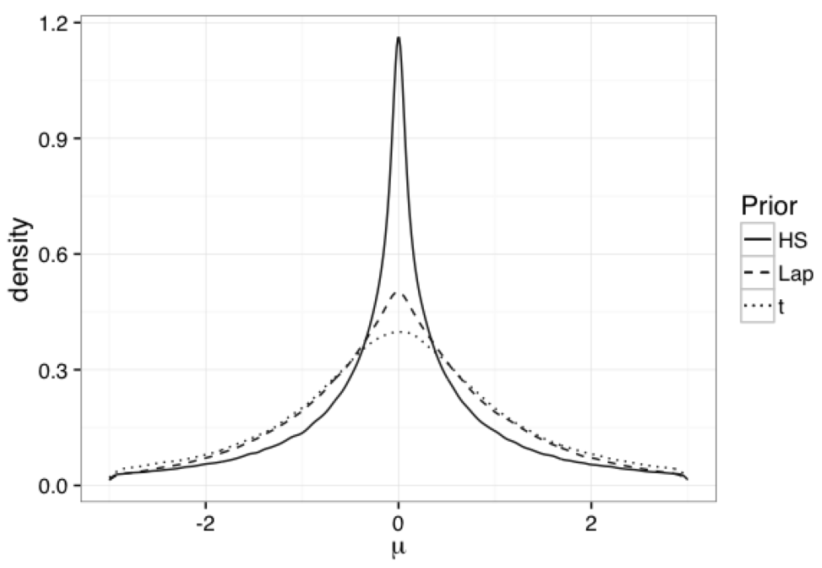The prior for ${\lambda }_j$ is set to be ${\lambda }_j\sim HalfCauchy(0,{\nu }_{\lambda }^j)$ for $j=1,\dots ,R$ ($\tau$ is set to be 1). As discussed in Section 2.2, these prior specifications of $\mathit{\beta }$ and ${\lambda }_j$ imply a horseshoe shrinkage on the coefficients ${\tilde{\mathit{\beta }}}_{.j}$’s. The prior for ${\eta }^2$ is ${\eta }^2\sim InverseGamma({\alpha }_h,{\beta }_h)$, where ${\alpha }_h$ and ${\beta }_h$ are scalars and pre-specified to be 4 and $0.01$, accordingly, to provide a reasonable mean and variance of ${\eta }^2$.

All priors are assumed to be independent. Based on the derived complete conditional posterior distributions for each parameter and latent variable, we obtain posterior samples using Metropolis–Hastings within Gibbs sampling since some conditional posterior distributions do not have closed forms. In estimation, we use the means of posterior samples as estimates for parameters and latent factors. Complete conditional posterior distributions for all model parameters and latent factors are provided in Appendix A.

3.2. Nowcasting Formulas

In this section, nowcasting formulas are provided. Suppose we are at $(q,T)$, the qth ($q=1,\dots ,Q$) releasing date in month T. As discussed in Section 3.1, the available information are $\{y_1,\dots ,y_K\}$ and $\{{\mathbf{x}}_1,\dots ,{\mathbf{x}}_{T_q},{\mathbf{x}}_{i\in v_{q,T_q+1}},\dots ,{\mathbf{x}}_{i\in v_{q,T}}\}$, here T can be the first ($T=3K+1$), second ($T=3K+2$), or third ($T=3K+3$) month of the quarter $K+1$. Our goal is to nowcast GDP $y_{K+1}$. Let ${\mathbf{A}}^{\left(g\right)}$, ${\beta }_0^{\left(g\right)}$, ${\mathit{\beta }}_i^{\left(g\right)}$ ($i=1,2,3$), ${\beta }_4^{\left(g\right)}$, ${\mathbf{A}}^{\left(g\right)}$, ${\mathbf{S}}^{\left(g\right)}=diag(\tau {\lambda }_1^{\left(g\right)},\dots ,\tau {\lambda }_R^{\left(g\right)})$, and ${\mathbf{F}}_t^{\left(g\right)}$ ($t=1,\dots ,T$) be the gth posterior draws for parameters and latent factors after the burn-in period, where $g=1,\dots ,G$. We nowcast $y_{K+1}$ using the following formulas.

• When $T=3K+1$, the nowcast of $y_{K+1}$ using BAY is given by:

  $$\begin{array}{cc}\hfill & {\widehat{y}}_{K+1}=\frac{1}{G}\sum _{g=1}^G[{\beta }_0^{\left(g\right)}+{\left({\mathit{\beta }}_{\mathbf{1}}^{\left(g\right)}\right)}^{\prime }{\mathit{S}}^{\left(g\right)}{\left({\mathbf{A}}^{\left(g\right)}\right)}^2{\mathbf{F}}_T^{\left(g\right)}+{\left({\mathit{\beta }}_{\mathbf{2}}^{\left(g\right)}\right)}^{\prime }{\mathit{S}}^{\left(g\right)}{\mathbf{A}}^{\left(g\right)}{\mathbf{F}}_T^{\left(g\right)}+\hfill \\ \hfill & {\left({\mathit{\beta }}_{\mathbf{3}}^{\left(g\right)}\right)}^{\prime }{\mathit{S}}^{\left(g\right)}{\mathbf{F}}_T^{\left(g\right)}+\left({\beta }_4^{\left(g\right)}\right)y_K],\hfill \end{array}$$

  (12)
• When $T=3K+2$, the nowcast of $y_{K+1}$ using BAY is given by:

  $$\begin{array}{cc}\hfill & {\widehat{y}}_{K+1}=\frac{1}{G}\sum _{g=1}^G[{\beta }_0^{\left(g\right)}+{\left({\mathit{\beta }}_{\mathbf{1}}^{\left(g\right)}\right)}^{\prime }{\mathit{S}}^{\left(g\right)}{\mathbf{A}}^{\left(g\right)}{\mathbf{F}}_T^{\left(g\right)}+{\left({\mathit{\beta }}_{\mathbf{2}}^{\left(g\right)}\right)}^{\prime }{\mathit{S}}^{\left(g\right)}{\mathbf{F}}_T^{\left(g\right)}+\hfill \\ \hfill & {\left({\mathit{\beta }}_{\mathbf{3}}^{\left(g\right)}\right)}^{\prime }{\mathit{S}}^{\left(g\right)}{\mathbf{F}}_{T-1}^{\left(g\right)}+\left({\beta }_4^{\left(g\right)}\right)y_K],\hfill \end{array}$$

  (13)
• When $T=3K+3$, the nowcast of $y_{K+1}$ using BAY is given by:

  $$\begin{array}{cc}\hfill & {\widehat{y}}_{K+1}=\frac{1}{G}\sum _{g=1}^G[{\beta }_0^{\left(g\right)}+{\left({\mathit{\beta }}_{\mathbf{1}}^{\left(g\right)}\right)}^{\prime }{\mathit{S}}^{\left(g\right)}{\mathbf{F}}_T^{\left(g\right)}+{\left({\mathit{\beta }}_{\mathbf{2}}^{\left(g\right)}\right)}^{\prime }{\mathit{S}}^{\left(g\right)}{\mathbf{F}}_{T-1}^{\left(g\right)}+\hfill \\ \hfill & {\left({\mathit{\beta }}_{\mathbf{3}}^{\left(g\right)}\right)}^{\prime }{\mathit{S}}^{\left(g\right)}{\mathbf{F}}_{T-2}^{\left(g\right)}+\left({\beta }_4^{\left(g\right)}\right)y_K].\hfill \end{array}$$

  (14)

Note that for some releasing dates, if $v_{q,T}=\varnothing$, meaning that no monthly series are available at releasing date $(q,T)$, then posterior samples ${\mathbf{F}}_T^{\left(g\right)}$ cannot be generated. As a solution, we use ${\tilde{\mathbf{F}}}_T^{\left(g\right)}={\mathbf{A}}^{\left(g\right)}{\mathbf{F}}_{T-1}^{\left(g\right)}$ to replace ${\mathbf{F}}_T^{\left(g\right)}$ in nowcasting equations. All of the parameter and factor estimations are updated in every single release within a month. Then, ${\widehat{y}}_{K+1}$ is re-produced for each release date.

4. Simulation Study

In this section, we will investigate three aspects of the Bayesian approach through numerical simulations. In Section 4.1, we evaluate whether it can successfully determine the true number of latent factors that can contribute to GDP nowcasting, i.e., the number of contributing factors. In Section 4.2, we study the accuracy of estimated latent factors ${\mathbf{F}}_t$. In Section 4.3, we examine out-of-sample nowcasting performances of the BAY approach.

In the simulation study, we simulate data following the model in Equations (1), (2) and (4) with $T=180$ (months), $K=60$ (quarters), $r=2$ (true number of contributing latent factors), $n=60$ (monthly series), and $Q=3$ release dates in each month. The releasing pattern follows Table 2 with 20 new monthly series released in each release date, that is: at $(1,T)$, release $({\mathbf{x}}_{41,T-2},\dots ,{\mathbf{x}}_{60,T-2})$, at $(2,T)$, release $({\mathbf{x}}_{21,T-1},\dots ,{\mathbf{x}}_{40,T-1})$ and at $(3,T)$, release $({\mathbf{x}}_{1,T},\dots ,{\mathbf{x}}_{20,T})$.

Table 2. Data releasing structure for simulation study when nowcasting quarter $K+1$’s GDP in month T. “RL” represents release. Orange color represents release 1, green represents release 2, and blue represents release 3.

Month	T-3	T-2	T-1	T
Series 1–20	Known	Known	Known	RL3
Series 21–40	Known	Known	RL2
Series 41–60	Known	RL1

Our method requires a predetermined cap R as the largest possible number of factors. Theoretically, R can be as large as the number of monthly series n. However, in practice, we use a smaller number to avoid extreme computational burden. In this simulation study, we choose $R=6$ because a preliminary PCA analysis shows that the first six principle components can explain at least $95\%$ of total variation for all six simulations. For all simulations, some of the parameter settings used in generating data are common: we set $\mathbf{A}=diag(0.9,-0.8,0.75,0.7,-0.65,0.6)$, $\mathbf{\Sigma }=diag(5.5,3,1,0.5,0.25,0.1)$; ${\beta }_0=0.5$, ${\mathit{\beta }}_i^{\prime }=(1,1,1,1,1,1)$ ($i=1,2,3$), ${\beta }_4=0.15$, and ${\eta }^2=1$. $\mathbf{\Omega }$ is simulated from $InverseWishart({60}^{-1}{\mathit{I}}_{60\times 60},60)$, each element of $\mathbf{\mu }$ equals to 10, and $\mathbf{\Theta }$ is simulated from $MatrixNormal(\mathsf{0},{\mathit{I}}_{60\times 60},{\mathit{I}}_{6\times 6})$.

Specifications of ${\lambda }_j$ ($j=1,\dots ,R$) for each of the simulation are shown in Table 3. For all six simulations, we assume only the first two factors majorly contribute to our nowcasting equations. Simulation 1 and Simulation 2 represent the group with high signals for the first two factors. Simulation 3 and Simulation 4 represent the group of moderate signals, while Simulation 5 and Simulation 6 are in the group of weak signals. Within each group, one of the simulations is configured with true sparsity, that is ${\lambda }_j=0$ for $j=3,\dots ,6$, while for another simulation, we assign non-sparsity with small noise (${\lambda }_j\sim N(0,0.1^2)$ for $j=3,\dots ,6$) as a comparison. In this way, we can investigate how our method performs when changing magnitudes of the true signals from strong to weak, and when the non-true signals are contaminated with small noise or not.

Table 3. Settings for ${\lambda }_j$. For each simulation, the first 2 factors are contributing factors, and other 4 factors contribute little or 0 to GDP prediction.

Simulation	${\mathit{\lambda }}_1$	${\mathit{\lambda }}_2$	${\mathit{\lambda }}_3,{\mathit{\lambda }}_4,{\mathit{\lambda }}_5,{\mathit{\lambda }}_6$
1	$N(5,{0.1}^2)$	$N(-5,{0.1}^2)$	$N(0,{0.1}^2)$
2	$N(5,{0.1}^2)$	$N(-5,{0.1}^2)$	0
3	$N(1,{0.1}^2)$	$N(-1,{0.1}^2)$	$N(0,{0.1}^2)$
4	$N(1,{0.1}^2)$	$N(-1,{0.1}^2)$	0
5	$N(0.1,{0.1}^2)$	$N(-0.1,{0.1}^2)$	$N(0,{0.1}^2)$
6	$N(0.1,{0.1}^2)$	$N(-0.1,{0.1}^2)$	0

For each simulation, we conduct one-step ahead nowcasts for the last 20 quarters using a moving window with a length of 10 years (40 quarters). For each quarter, nowcasting is made in each release date within each month. Thus, there are $20\left(quarters\right)\times 3\left(months\right)\times 3\left(releasedates\right)=180$ nowcasts in each simulation. In our MCMC procedure, we discard the first 10,000 iterations as burn-in and run 1000 more for posterior summaries.

4.1. Estimating the Number of Contributing Factors

In this section, we validate our Bayesian Approach’s ability in determining true number of contributing factors through six sets of simulation studies. The ability of the algorithm to determine the true number of contributing factors is investigated as follows. First, we check whether our approach can perform as expected when true signals of the first two factors are high, moderate, and low, and the non-true signals are exactly equal to 0. Secondly, we check if its performance will be undermined if we add some noise to the non-true signals.

For each simulation, every estimate of the shrinkage profiles ${\widehat{\kappa }}_j$ ($j=1,\dots ,R$) is calculated using the average of 1000 posterior draws after the burn-in period, that is ${\widehat{\kappa }}_j={\sum }_{g=1}^G{\kappa }_j^{\left(g\right)}={\sum }_{g=1}^G\frac{1}{1+{\lambda }_j^{\left(g\right)}}$ for $G=1000$. Figure 3 shows box-plots of estimated shrinkage profiles ${\widehat{\kappa }}_j$ ($j=1,\dots ,R$) based on 180 nowcast estimates in each simulation. In Simulation 1 and Simulation 2, ${\widehat{\kappa }}_1$ and ${\widehat{\kappa }}_2$ are near 0 while ${\widehat{\kappa }}_3$ to ${\widehat{\kappa }}_6$ are generally close to 1, indicating that the algorithm can successfully detect high signals for the first two contributing factors and shrink the other four to zero. In Simulation 3 and Simulation 4, when we decrease signals of the first two factors from high to moderate, our algorithm can still detect signals of the first two and shrinkage signals of the last four to 0. However, if we only apply low signals for the first two factors, as shown in Simulation 5 and Simulation 6, the algorithm can only detect one contributing factor while shrinking all others to 0. When comparing results between right column (Simulation 2, 4, and 6 for true sparsity) and left column (Simulation 1, 3, and 5 for small noise), our algorithm can extremely shrink all four non-true factors (i.e., having ${\widehat{\kappa }}_j\approx 1$) in all three scenarios with different strengths of true signals, disregarding whether the non-true factors are contaminated with noise or not. The findings in Figure 3 validate our algorithm’s ability to detect the true number of contributing factors with moderate to high signals.

Figure 3. Box-plots of shrinkage profile estimations ${\widehat{\kappa }}_j$ for $j=1,\dots ,R$ from 180 nowcast estimates. Here, $R=6$. Each subplot represents the result for each simulation.

Figure 4 shows a scatterplot of posterior means ${\widehat{\kappa }}_{ij}$’s (${\widehat{\kappa }}_{ij}={\widehat{\kappa }}_j)$ versus ${\widehat{\tilde{\beta }}}_{ij}$’s from 180 nowcast estimates. There are two general patterns observed across all six simulations. The first is that the estimated profile ${\widehat{\kappa }}_{ij}$’s get closer to zero (little shrinkage) when the values of ${\widehat{\tilde{\beta }}}_{ij}$’s increase horizontally to very large numbers, while ${\widehat{\kappa }}_{ij}$’s approach to one (strong shrinkage) when ${\widehat{\tilde{\beta }}}_{ij}$’s become very small. The second pattern is that the dots are separated into two clear segmentations in each picture. The vertical distance between two groups is the largest for the strong signal cases (Simulation 1 and 2), then becomes smaller for the moderate signals (Simulation 3 and 4). However, for the last row (the weak signal cases), the distance almost diminishes. This is consistent with the findings in Figure 3.

Figure 4. Scatter splots of shrinkage profile estimations ${\widehat{\kappa }}_{ij}$ (y-axis) versus ${\widehat{\tilde{\beta }}}_{ij}$ (x-axis) from 180 nowcast estimates. Each subplot represents the result for each simulation.

4.2. Estimation of Latent Factors

We then investigate whether the BAY method can accurately estimate the latent factors ${\mathbf{F}}_t$. In our approach, latent variables ${\mathbf{F}}_t$ are also estimated with posterior means, i.e., ${\widehat{\mathbf{F}}}_t=\frac{1}{G}{\sum }_{g=1}^G{\mathbf{F}}_t^{\left(g\right)}$, $t=1,\dots ,T$, and $G=1000$ is the number of MCMC iterations after the burn-in period. Figure 5 plots the estimated first two latent factors from BAY approach, together with the true latent factors, in the first 100 months (in-sample period) of the data for six simulations. The absolute values are compared since the factors are identified up to a change of sign (Section 2.1). Figure 5 shows that, generally, the estimation from the BAY approach is close to the true factors, especially for the first four simulations in which the true number of contributing latent factors is successfully detected.

Figure 5. In-sample fit of the latent factors for 6 simulations. Absolute value is used for both true factors and in-sample fits. Yellow lines represent in-sample fitted value and gray lines represent true value. In each subplot, the upper panel represents the comparison for the first factor, and the lower panel shows the comparison for the second factor.

4.3. Out-of-Sample Nowcasting Performances

In this section, we prove that our Bayesian Apporach can provide exceptional out-of-sample nowcasting performances compared to the Random Walk.

Out-of-sample nowcasting performances are assessed based on 20 one-step-ahead nowcasting. For each simulation, whenever there are new series released in a month, the model parameters and latent factors will be updated. Therefore, there are 180 nowcasts in total.

Figure 6 presents the nowcasting performances for all six simulations. In each panel (representing each simulation), the first, second, and third row represent nowcasting trends over 20 quarters in the first, second, and third month, respectively. In each subplot of each panel, the black curve represents the true GDP, while colored curves with different symbols represent nowcasts from different releases. Figure 6 shows that BAY approach can capture trends and changes in simulated GDP really well. For all six simulations, within the same month, there is no obvious difference in nowcasting performance between release 1 and release 2. However, nowcasting curves for release 3 are slightly closer to true curves than that of the other two releases. Moreover, we can see obvious improvements from nowcasts in the first month to nowcasts in the third month.

Figure 6. Nowcasting performance for six simulations. Three rows in each subplot represent the first, second, and third month’s nowcasts for the last 20 quarters, respectively. Black curve represents true simulated GDP, and colored curves with different shapes represent nowcasts from different releases.

In order to better understand nowcasting results, we use mean absolute nowcasting error (MANE) to measure nowcasting accuracy. Let ${\widehat{y}}_{K+1}^{q,T}$ be the nowcast at qth release date of month T, where $q=1,2,3$ and $T=3K+1,3K+2,3K+3$. Then, $\mathit{MANE}(q,T)=\frac{1}{20}{\sum }_{k+1=41}^{60}|{\widehat{y}}_{k+1}^{q,T}-y_{k+1}|$. We compare the nowcasting performances of BAY with that of the random walk (RW) approach, which uses the previous quarter GDP to predict the current quarter GDP, by calculating MANE reduction relative to RW (i.e., $\frac{\mathit{MANE}(q,T)-{\mathit{MANE}}^{\mathit{rw}}}{{\mathit{MANE}}^{\mathit{rw}}}$). Table 4 provides MANE reductions (in percentage) for BAY approach compared with that of the RW. For instance, $-30\%$ indicates that BAY can reduce $30\%$ of MANE of the RW. Table 4 shows that, moving from the first month to the third month, there are significant reductions in terms of MANE ratios. Within each month, there is no obvious difference in MANE ratios between release 1 and release 2, while release 3 can provide larger MANE reduction than the other two. The possible reason is that, in the releasing pattern of this simulation study, series of the current month are only released in the third release of each month.

Table 4. This table reports percentages of reduction in MANE relative to RW, which are calculated as $({\mathit{MANE}}^{\mathit{Bay}}-{\mathit{MANE}}^{\mathit{RW}})/{\mathit{MANE}}^{\mathit{RW}}\times 100\%$, for six simulation studies.

Simulation	1			2
Release	1st Month	2nd Month	3rd Month	1st Month	2nd Month	3rd Month
1st	$-15.4\%$	$-35.9\%$	$-55.5\%$	$-35.2\%$	$-50.6\%$	$-81.4\%$
2nd	$-16.4\%$	$-34.6\%$	$-56.5\%$	$-34.6\%$	$-51.1\%$	$-80.4\%$
3rd	$-32.8\%$	$-54.6\%$	$-96.6\%$	$-53.3\%$	$-82.3\%$	$-97.3\%$
Average	$-21.5\%$	$-41.7\%$	$-69.5\%$	$-41.0\%$	$-61.3\%$	$-86.4\%$
Simulation	3			4
Release	1st Month	2nd Month	3rd Month	1st Month	2nd Month	3rd Month
1st	$-24.6\%$	$-52.5\%$	$-68.7\%$	$-43.5\%$	$-53.5\%$	$-73.1\%$
2nd	$-24.5\%$	$-54.7\%$	$-69.3\%$	$-44.5\%$	$-55.1\%$	$-73.3\%$
3rd	$-51.5\%$	$-68.2\%$	$-89.0\%$	$-57.9\%$	$-75.1\%$	$-90.7\%$
Average	$-33.5\%$	$-58.5\%$	$-75.7\%$	$-48.6\%$	$-61.2\%$	$-79.0\%$
Simulation	5			6
Release	1st Month	2nd Month	3rd Month	1st Month	2nd Month	3rd Month
1st	$-33.5\%$	$-29.4\%$	$-50.5\%$	$-25.5\%$	$-43.9\%$	$-66.0\%$
2nd	$-34.9\%$	$-28.3\%$	$-49.4\%$	$-25.3\%$	$-43.1\%$	$-66.2\%$
3rd	$-27.7\%$	$-52.3\%$	$-62.7\%$	$-44.5\%$	$-66.0\%$	$-69.9\%$
Average	$-32.0\%$	$-36.7\%$	$-54.2\%$	$-31.8\%$	$-51.0\%$	$-67.4\%$

In summary, this simulation study suggests that our BAY approach can successfully detect true number of contributing factors with moderate to high signals. It also has the ability to estimate latent dynamic factors accurately and produce reliable nowcasting results.

5. Empirical Study

In this section, we examine empirical performance of the BAY method using U.S. quarterly GDP growth rates. The Federal Reserve Bank of New York built a platform that has been nowcasting U.S. GDP growth rates since April 2016. The methodology behind the platform is based on the GRS method, and details can be found in Bok et al. [18]. We borrow their data from Github (https://github.com/FRBNY-TimeSeriesAnalysis/Nowcasting) in 20 April 2021. This data set contains 26 monthly series released by both government agencies and private institutions. Based on economic insights, those monthly series are assigned to nine different categories, such as labor, international trade, manufacturing, surveys, and others. All series are updated in real time; thus, the release dates for each one vary from month to month. Based on the approximate release dates for each individual series, we roughly group these series into three release dates: before 10th, from 10th to 20th, and after the 20th of a month. Table 5 provides the release pattern of the real data. The same transformations as in Bok et al. [18] are applied to monthly series to achieve stationarity. Detailed information of transformations and release patterns are available in Table 6 and Table 7.

Table 5. Data releasing structure in the empirical study when nowcasting quarter $K+1$’s GDP in month T. RL stands for release, with release 1 colored in orange, released 2 colored in green, and release 3 colored in blue. The number in parentheses represents number of series for that particular release.

Month	T-3	T-2	T-1	T
Set 1 (2)	Known	Known	Known	RL2 (2)
Set 2 (2)	Known	Known	RL1 (2)
Set 3 (10)	Known	Known	RL2 (10)
Set 4 (7)	Known	Known	RL3 (7)
Set 5 (5)	Known	RL1 (5)
Set 6 (3)	Known	RL2 (3)

Table 6. Data transformation types: $x_{it}^{\ast }$ represents raw data, and $x_{it}$ represents the transformed data.

Type	Transformation	Description
1	$x_{it}=x_{it}^{\ast }$	No transformation
2	$x_{it}=x_{it}^{\ast }-x_{i,t-1}^{\ast }$	Level change
3	$x_{it}=\frac{x_{it}^{\ast }-x_{i,t-1}^{\ast }}{x_{i,t-1}^{\ast }}$	Month-to-month change

Table 7. Release groups, transformation types, and lag information for monthly series used in the empirical study.

Release	Block	Name	Transformation	Lag
1st	Housing and construction	TTLCONS	3	2
	International trade	BOPTEXP	3	2
		BOPTIMP	3	2
	Manufacturing	BUSINV	3	2
	Labor	PAYEMS	2	1
		JTSJOL	2	2
		UNRATE	2	1
2nd	International trade	IR	3	1
		IQ	3	1
	Retail and consumption	RSAFS	3	1
	Survey	GACDISA066MSFRBNY	1	0
		GACDFSA066MSFRBNY	1	0
	Manufacturing	INDPRO	3	1
		TCU	2	1
	Other	CPIAUCSL	3	1
		CPILFESL	3	1
		PPIFIS	3	1
	Housing and construction	HOUST	3	1
		PERMIT	2	1
3rd	Manufacturing	DGORDER	3	1
		WHLSLRIMSA	3	1
	Housing and construction	HSNIF	3	1
	Income	DSPIC96	3	1
	Retail and consumption	PCEC96	3	1
	Other	PCEPI	3	1
		PCEPILIFE	3	1

We choose the data span from 1993Q1 to 2016Q4, which gives us data series with 288 months (96 quarters). In-sample data is chosen to be in the period from 1993Q1 to 2002Q4, while the nowcasting horizon covers 2003Q1 to 2016Q4. The GDP growth rate used in this empirical study is the annualized quarter over quarter percentage change, which is defined as:

$$Y_k=\{{(1+\frac{{\mathit{GDP}}_k-{\mathit{GDP}}_{k-1}}{{\mathit{GDP}}_{k-1}})}^4-1\}\times 100,$$

where ${\mathit{GDP}}_k$ is the real GDP of quarter k. Figure 7 plots the GDP growth rate with nowcasting horizon on the right side of the dashed blue line. In Figure 7, we see a severe drop at around 2009Q1 which is due to the financial crisis around 2007–2008.

Figure 7. Real U.S. GDP growth rate from 1993Q1 to 2016Q4. Period after 2003Q1 (after blue dashed line) is the nowcasting horizon.

We apply our BAY approach to this real U.S. GDP data. In this empirical study, we assign the same prior settings as in the simulation study; the largest possible number of latent factors R is also assumed to be six as the first six principle components from PCA explain $99.9\%$ of the variation observed in monthly series, and we still use $G=1000$ iterations after 10,000 burn-in period in the MCMC sampling. Estimations of shrinkage profiles ${\widehat{\kappa }}_j$ are used to determine the number of contributing factors. Out of all $56\left(quarters\right)\times 3\left(months\right)\times 3\left(releases\right)=504$ estimates of shrinkage profiles, we find there are two main scenarios occurring. Figure 8 plots two examples for each of them, respectively. The left panel is the boxplot for posterior draws of shrinkage profile ${\widehat{\kappa }}_j$’s when nowcasting 2000Q4 in the first release of the first month. This plot shows that the first factor is clearly detected to be different from the other five factors, although its $\widehat{\kappa }$ value is not small. The right panel is the boxplot for ${\widehat{\kappa }}_j$’s when nowcasting 2000Q2 in the first release of the first month. This plot, however, shows that no factor contributes to the GDP nowcasting.

Figure 8. Two examples of boxplots for posterior draws of ${\kappa }_j$. Left panel represents the one for nowcasting GDP of 2000Q4 in the first release of the first month. Right panel represents the one for nowcasting GDP of 2000Q2 in the first release of the first month.

Table 8 shows proportions of all nowcasts in which one factor is detected. Generally speaking, more than $50\%$ of cases have one factor detected to have contribution for GDP nowcasting. This is consistent with Bok et al. [18], where they assume one single common factor in their DFMs setting.

Table 8. This table reports percentages of nowcasts in which one factor is detected.

Method	BAY
Release	1st Month	2nd Month	3rd Month
1st	$50\%$	$46.4\%$	$62.5\%$
2nd	$58.9\%$	$50\%$	$58.9\%$
3rd	$46.4\%$	$62.5\%$	$55.3\%$
Average	$51.7\%$	$52.9\%$	$58.9\%$

Figure 9 plots out-of-sample GDP nowcasts over last 56 quarters for each release in each month. Three rows represents three nowcasting months. In this plot, we compare our BAY approach with the autoregressive model of order 1 (AR(1)) $y_k={\beta }_0+{\beta }_4{y}_{k-1}+{\nu }_k$. The AR(1) is equivalent to the case where no factor is detected. Figure 9 shows that our BAY approach can successfully capture the economic downfall due to the financial crisis at 2009Q1 with one lag delay. However, the AR(1) failed to capture it.

Figure 9. Nowcasting over 2003Q1 to 2016Q4. Three rows represent three nowcasting months, respectively. Black curve represents the real GDP, while curves of different colors and shapes represent nowcasting results from 3 different release dates and AR(1).

For the empirical study, we calculate MANE to measure nowcasting errors. Here, apart from AR(1), we also compare our BAY approach with another Bayesian model with no shrinkage priors, and we refer this model as NS. The NS model is proposed as the following: keep all other settings the same and remove $\mathit{S}$ from Equation (5). More specifically, in the NS model, we impose Normal priors on the ${\tilde{\mathit{\beta }}}_{.j}$’s instead of horseshoe priors. Table 9 provides MANE reductions of BAY approach, relative to RW, AR(1), and NS. The first sub-table reports the percentage of reduction in MANEs relative to RW accross three nowcasting months, while the middle sub-table reports the percentage of reduction in MANEs relative to AR(1), and the last sub-table reports the percentage of reduction in MANEs relative to NS. Table 9 shows that our BAY approach can produce smaller nowcasting errors than the RW approach. On average, the percentages of reduction relative to RW do not have an obvious difference from first month to third month. This indicates that, for real data, having more monthly series does not necessarily lead to better nowcasting performances. One potential reason is that the quality of the data might not be perfect. Adding more series means adding more noise and thus may not guarantee more accurate nowcasts of GDP. The MANE reduction relative to AR(1) are lower than those relative to RW. However, our BAY approach can still have approximately $11\%$ reduction in nowcasting errors when being compared with the AR(1). This indicates that even if no factor is detected in nearly $50\%$ of the cases, the ones with one factor detected indeed contribute and enhance our nowcasting performance. The MANE reduction relative to NS for the first two nowcasting months are comparable and are lower than those relative to AR(1), the MANE reduction for the third month is higher than those relative to AR(1). This result indicates that using the horseshoe shrinkage idea to shrink unimportant factors to 0 can further increase our model’s nowcasting performance.

Table 9. This table reports percentages of reduction in MANE’s relative to RW, AR(1), and NS, i.e., $({\mathit{MANE}}^{\mathit{Bay}}-{\mathit{MANE}}^{\ast })/{\mathit{MANE}}^{\ast }\times 100\%$, here * can be RW, AR(1), or NS.

Compare with	RW
Release	1st Month	2nd Month	3rd Month
1st	$-20.6\%$	$-27.5\%$	$-32.0\%$
2nd	$-28.4\%$	$-21.9\%$	$-19.2\%$
3rd	$-25.0\%$	$-23.9\%$	$-24.7\%$
Average	$-24.7\%$	$-24.4\%$	$-25.3\%$
Compare with	AR(1)
Release	1st Month	2nd Month	3rd Month
1st	$-14.0\%$	$-14.2\%$	$-19.5\%$
2nd	$-15.3\%$	$-7.65\%$	$-4.38\%$
3rd	$-11.2\%$	$-8.97\%$	$-10.9\%$
Average	$-13.5\%$	$-10.3\%$	$-11.6\%$
Compare with	NS
Release	1st Month	2nd Month	3rd Month
1st	$-1.90\%$	$0.70\%$	$-19.8\%$
2nd	$-8.51\%$	$-7.32\%$	$-10.1\%$
3rd	$-9.21\%$	$-12.4\%$	$-9.79\%$
Average	$-6.54\%$	$-6.34\%$	$-13.23\%$

In summary, this empirical analysis demonstrates the empirical relevance of the BAY approach in nowcasting U.S. GDP. It suggests that at most one factor is sufficient for our BAY approach to provide a good performance.

6. Conclusions

Real-time nowcasting has become important in making policy decisions and long-term forecasting. In this paper, we adopt the DFM model framework and introduce a Bayesian MCMC approach for real-time nowcasting. Unlike other nowcasting methods based on DFMs, our Bayesian approach allows an unknown number of contributing factors and utilizes the horseshoe shrinkage to determine the number of contributing factors. Through the simulation study, we have shown that our Bayesian approach can identify the number of contributing factors correctly with high to moderate signals and estimate latent factors accurately. Both simulation study and empirical study validate our Bayesian approach’s ability to provide reliable real-time nowcasting results.

In this paper, we are not able to add the horseshoe shrinkage to Equation (1) due to the non-identifiable issue in DFMs. If we add $\mathbf{S}$ as $\mathbf{\Theta }\mathbf{S}{\mathbf{F}}_t$ in Equation (1), there will be two layers of non-identifiable issues, which is difficult to solve. Furthermore, in this paper, the horseshoe shrinkage is only used in detecting the number of contributing factors. In our DFMs framework, we assume the GDP of quarter k depends on factors with up to two lags, i.e., factors of $3k$, $3k-1$, and $3k-2$ (see Equation (3)). We might argue that this lag should not be fixed and can also be determined using the horseshoe shrinkage. These are two possible research directions that we want to explore in future investigation.

Appendix A.1. Posterior Samples for Mean of Monthly Series μ

The conditional posterior for the mean of monthly series, $\mathbf{\mu }$, is a multivariate normal distribution:

$$\mathbf{\mu }|\mathit{X},\mathbf{F},\mathbf{\Theta },\mathbf{\Omega }\sim N({\mathbf{U}}_{\mu },{\mathbf{\Sigma }}_{\mu }),$$

(A1)

where

$$\begin{array}{cc}\hfill & {\mathbf{\Sigma }}_{\mu }^{-1}=T_q{\mathbf{\Omega }}^{-1}+\sum _{t=T_q+1}^T\left({\mathbf{1}}_{v_{q,t}}^{\prime }{\left({\mathbf{1}}_{v_{q,t}}\mathbf{\Omega }{\mathbf{1}}_{v_{q,t}}^{\prime }\right)}^{-1}{\mathbf{1}}_{v_{q,t}}\right)+{\mathbf{I}}_{n\times n},\hfill \\ \hfill & {\mathbf{U}}_{\mu }={\mathbf{\Sigma }}_{\mu }\left[\sum _{t=1}^{T_q}{\mathbf{\Omega }}^{-1}(x_t-\mathbf{\Theta }{\mathbf{F}}_t)+\sum _{t=T_q+1}^T\left({\mathbf{1}}_{v_{q,t}}^{\prime }{\left({\mathbf{1}}_{v_{q,t}}\mathbf{\Omega }{\mathbf{1}}_{v_{q,t}}^{\prime }\right)}^{-1}{\mathbf{1}}_{v_{q,t}}\right)(x_t-\mathbf{\Theta }{\mathbf{F}}_t)\right].\hfill \end{array}$$

Appendix A.2. Posterior Samples for Factor Loading Matrix Θ

Let $\mathbf{\theta }=vec\left(\mathbf{\Theta }\right)={({\theta }_1,\dots ,{\theta }_n)}^{\prime }$. The conditional posterior for the $\mathbf{\theta }$ is a multivariate normal distribution:

$$\mathbf{\theta }|\mathit{X},\mathbf{F},\mathbf{\mu },\mathbf{\Omega }\sim N({\mathbf{U}}_{\theta },{\mathbf{\Sigma }}_{\theta }),$$

(A2)

let ${\mathbf{C}}_t={\mathbf{I}}_{n\times n}\otimes {\mathbf{F}}_t$, then

$$\begin{array}{cc}\hfill & {\mathbf{\Sigma }}_{\theta }^{-1}=\sum _{t=1}^{T_q}{\mathbf{C}}_t^{\prime }{\mathbf{\Omega }}^{-1}{\mathbf{C}}_t+\sum _{t=T_q+1}^T{\mathbf{C}}_t^{\prime }{\mathbf{1}}_{v_{q,t}}^{\prime }{\left({\mathbf{1}}_{v_{q,t}}\mathbf{\Omega }{\mathbf{1}}_{v_{q,t}}^{\prime }\right)}^{-1}{\mathbf{1}}_{v_{q,t}}{\mathbf{C}}_t+{\mathbf{I}}_{nR\times nR},\hfill \\ \hfill & {\mathbf{U}}_{\theta }={\mathbf{\Sigma }}_{\theta }\left[\sum _{t=1}^{T_q}{\mathbf{C}}_t^{\prime }{\mathbf{\Omega }}^{-1}(x_t-\mathbf{\mu })+\sum _{t=T_q+1}^T{\mathbf{C}}_t^{\prime }{\mathbf{1}}_{v_{q,t}}^{\prime }{\left({\mathbf{1}}_{v_{q,t}}\mathbf{\Omega }{\mathbf{1}}_{v_{q,t}}^{\prime }\right)}^{-1}{\mathbf{1}}_{v_{q,t}}(x_t-\mathbf{\mu })\right].\hfill \end{array}$$

Appendix A.3. Posterior Samples for Covariance in Monthly Series Ω

The conditional posterior for $\mathbf{\Omega }$ is

$$\begin{array}{cc}\hfill & p\left(\mathbf{\Omega }\right|·)\propto \prod _{t=1}^{T_q}p\left({\mathbf{x}}_t\right|\mu ,{\mathbf{F}}_t,\theta ,\mathbf{\Omega })\times \prod _{t=T_q+1}^{T}p\left({\mathbf{1}}_{v_{q,t}}{\mathbf{x}}_t\right|\mu ,{\mathbf{F}}_t,\theta ,\mathbf{\Omega })\times P\left(\mathbf{\Omega }\right)\hfill \\ \hfill & \propto {\left|\mathbf{\Omega }\right|}^{-(T_q-1)/2}{e}^{-\frac{1}{2}tr\left[{\sum }_{t=1}^{T_q}(x_t-\mu -{\mathbf{C}}_t\theta ){(x_t-\mu -{\mathbf{C}}_t\theta )}^{\prime }{\mathbf{\Omega }}^{-1}\right]}\hfill \\ \hfill & \times {\left|\mathbf{\Omega }\right|}^{-({\nu }_{\theta }+n+1)/2}{e}^{-\frac{1}{2}tr\left[\frac{1}{n}{\mathbf{\Omega }}^{-1}{\mathit{I}}_{n\times n}\right]}\hfill \\ \hfill & \times \prod _{t=T_q+1}^T{\left|{\mathbf{1}}_{v_{q,t}}\mathbf{\Omega }{\mathbf{1}}_{v_{q,t}}^{\prime }\right|}^{-\frac{1}{2}}{e}^{-\frac{1}{2}tr\left[{\mathbf{1}}_{v_{q,t}}(x_t-\mu -{\mathbf{C}}_t\theta ){\mathbf{1}}_{v_{q,t}}^{\prime }{(x_t-\mu -{\mathbf{C}}_t\theta )}^{\prime }{\left({\mathbf{1}}_{v_{q,t}}\mathbf{\Omega }{\mathbf{1}}_{v_{q,t}}^{\prime }\right)}^{-1}\right]},\hfill \end{array}$$

(A3)

which is not in a closed form. We need to use Metropolis–Hastings within Gibbs sampling method to draw $\mathbf{\Omega }$. The first two parts combined together yield an inverse Wishart distribution ${\mathit{W}}^{-1}({\mathbf{\Phi }}_{\mathsf{\Omega }},{\nu }_{\mathsf{\Omega }})$, with ${\mathbf{\Phi }}_{\mathsf{\Omega }}=\frac{1}{n}{\mathit{I}}_{n\times n}+{\sum }_{t=1}^{T_q}(x_t-\mathbf{\mu }-{\mathbf{C}}_t\theta ){(x_t-\mathbf{\mu }-{\mathbf{C}}_t\theta )}^{\prime }$ and ${\nu }_{\mathsf{\Omega }}=T_q+{\nu }_{\theta }$. Therefore, we purpose ${\mathbf{\Omega }}^{\ast }$ from ${\mathit{W}}^{-1}({\mathbf{\Phi }}_{\mathsf{\Omega }},{\nu }_{\mathsf{\Omega }})$ and use the last piece in the posterior distribution, denoted as $q\left(\mathbf{\Omega }\right)$, to construct the acceptance–rejection rate. That is, the proposal ${\mathbf{\Omega }}^{\ast }$ is accepted with probability

$$P\left({\mathbf{\Omega }}^{\ast }\right|{\mathbf{\Omega }}^0)=min\left\{1,\frac{q\left({\mathbf{\Omega }}^{\ast }\right)}{q\left({\mathbf{\Omega }}^0\right)}\right\},$$

where ${\mathbf{\Omega }}^0$ denotes the current state of $\mathbf{\Omega }$.

Appendix A.4. Posterior Samples for AR(1) Coefficients a_j

For $j=1,\dots ,R$, the conditional posterior of each $AR\left(1\right)$ coefficient $a_j$ is:

$$a_j|\mathbf{F},\mathbf{\Sigma }\sim N({\mu }_{a_j},{\sigma }_{a_j^2})I\left(\right|a_j|<1),$$

(A4)

where ${\mu }_{a_j}=\frac{{\sum }_{t=2}^T{f}_{j,t}{f}_{j,t-1}}{{\sigma }_j^2+{\sum }_{t=2}^T{f}_{j,t-1}^2}$ and ${\sigma }_{a_j^2}=\frac{{\sigma }_j^2}{{\sigma }_j^2+{\sum }_{t=2}^T{f}_{j,t-1}^2}$.

Appendix A.5. Posterior Samples for Covariance Matrix in the Factor Equation Σ

For $j=1,\dots ,R$, the conditional posterior of each diagonal element of $\mathbf{\Sigma }$, ${\sigma }_j^2$, is an inverse gamma distribution:

$${\sigma }_j^2|\mathit{F},\mathit{A}\sim iG({\alpha }_j,{\beta }_j),$$

(A5)

where ${\alpha }_j={\alpha }_s+(T-1)/2$ and ${\beta }_j={\beta }_s+{\sum }_{t=2}^T{(f_{j,t}-a_j{f}_{j,t-1})}^2/2$.

Appendix A.6. Posterior Samples for Coefficients in GDP Equation β

The conditional posterior of coefficients connecting factors with GDP, $\mathit{\beta }$, is a multivariate normal distribution:

$$\mathit{\beta }|\mathit{F},y_2,\dots ,y_K,{\eta }^2\sim N({\mathbf{U}}_{\beta },{\mathbf{\Sigma }}_{\beta }),$$

(A6)

where ${\tilde{\mathit{F}}}_{3k}={[1,{\left(\mathbf{S}{\mathit{F}}_{3k}\right)}^{\prime },{\left(\mathbf{S}{\mathit{F}}_{3k-1}\right)}^{\prime },{\left(\mathbf{S}{\mathit{F}}_{3k-2}\right)}^{\prime },y_{k-1}]}^{\prime }$, and

$$\begin{array}{cc}\hfill & {\mathbf{\Sigma }}_{\beta }^{-1}=\sum _{k=2}^K{\tilde{\mathit{F}}}_{3k}{\tilde{\mathit{F}}}_{3k}^{\prime }/{\eta }^2+{\mathit{I}}_{(3R+2)\times (3R+2)},\hfill \\ \hfill & {\mathbf{U}}_{\beta }={\mathbf{\Sigma }}_{\beta }\sum _{k=2}^K{\tilde{\mathit{F}}}_{3k}{y}_k/{\eta }^2,\hfill \end{array}$$

where $\mathbf{S}=diag({\lambda }_1,\dots ,{\lambda }_R)$.

Appendix A.7. Posterior Samples for Variance in GDP Equation η²

The conditional posterior of the variance in GDP equation, ${\eta }^2$, is an inverse gamma distribution:

$${\eta }^2|\mathit{F},y_2,\dots ,y_K,\beta ,\mathit{S}\sim iG({\alpha }_{\eta },{\beta }_{\eta }),$$

(A7)

where ${\alpha }_{\eta }={\alpha }_h+(K+1)/2$, and ${\beta }_{\eta }={\beta }_h+{\sum }_{k=2}^K{(y_k-{\beta }^{\prime }{\tilde{\mathit{F}}}_{3k})}^2/2$.

Here, ${\tilde{\mathit{F}}}_{3k}={[1,{\left(\mathbf{S}{\mathit{F}}_{3k}\right)}^{\prime },{\left(\mathbf{S}{\mathit{F}}_{3k-1}\right)}^{\prime },{\left(\mathbf{S}{\mathit{F}}_{3k-2}\right)}^{\prime },y_{k-1}]}^{\prime }$, and $\mathbf{S}=diag({\lambda }_1,\dots ,{\lambda }_R)$.

Appendix A.8. Posterior Samples for Each Element in S Matrix, λ_j

For simplicity, we assume $\tau =1$. The posterior for ${\lambda }_j$ is

$$\begin{array}{cc}\hfill & p\left({\lambda }_j\right|·)\propto \prod _{l=1}^{3}p\left({\mathit{\beta }}_{\mathit{l}}\right|·)\times P\left({\lambda }_j\right)\hfill \\ \hfill & \propto \frac{1}{{\lambda }_j^3}exp\{-\frac{1}{2}\sum _{l=1}^3{\beta }_{lj}^2{\lambda }_j^{-2}\}\times \frac{1}{1+\frac{{\lambda }_j^2}{{\nu }_{\lambda }^{2j}}},\hfill \end{array}$$

(A8)

where ${\beta }_{lj}$ is the jth element in ${\mathit{\beta }}_l$ for $l=1,2,3$. This posterior does not have a closed form, and the Metropolis–Hastings within Gibbs sampling method is required to draw ${\lambda }_j$. If we define ${\tilde{\lambda }}_j:={\lambda }_j^{-2}$, the first part of the posterior yields a gamma distribution for ${\tilde{\lambda }}_j$, i.e., ${\tilde{\lambda }}_j\sim Gamma(2.5,\frac{2}{{\sum }_{l=1}^3{\beta }_{lj}^2})$. Therefore, we purpose ${\tilde{\lambda }}_j^{\ast }$ from $Gamma(2.5,\frac{2}{{\sum }_{l=1}^3{\beta }_{lj}^2})$, obtain ${\lambda }_j^{\ast }={\tilde{\lambda }}_j^{\ast -\frac{1}{2}}$, and use the last piece in the conditional posterior distribution $q\left({\lambda }_j\right)=\frac{1}{1+\frac{{\lambda }_j^2}{{\nu }_{\lambda }^{2j}}}$ to construct the acceptance–rejection rate. That is, the proposal ${\lambda }_j^{\ast }$ is accepted with probability

$$P\left({\lambda }_j^{\ast }\right|{\lambda }_j^0)=min\left\{1,\frac{q\left({\lambda }_j^{\ast }\right)}{q\left({\lambda }_j^0\right)}\right\},$$

where ${\lambda }_j^0$ denotes the current state of ${\lambda }_j$.

Appendix A.9. Sampling the Latent Factors F_t

The posterior distribution for ${\mathit{F}}_t$ has different forms depending on t. Suppose $K^{\ast }$ is the largest integer such that $3K^{\ast }\le T_q$, $T_q$, as defined in Section 2. For $3<t<3K^{\ast }$, we have the most general form defined as follows:

First, we write t as $t=3(k-1)+i$ for $k=2,\dots ,K^{\ast }$, where $i=1,2,3$ represents that we are in the first, second, and third month of quarter k. Then, at $t=3(k-1)+i$, ${\mathit{F}}_t$ enters the joint likelihood through $x_t$, ${\mathit{F}}_{t+1}$,${\mathit{F}}_{t-1}$ and $y_k$ by

$$\left(\begin{array}{c}{x}_t\\ {\mathit{F}}_{t+1}\\ {\mathit{F}}_{t+1}\\ f_{y_k}\left(i\right)\end{array}\right)=\left(\begin{array}{c}\mathbf{\Theta }\\ \mathit{A}\\ {\mathit{A}}^{-1}\\ {\beta }_i^{\prime }\mathit{S}\end{array}\right){\mathit{F}}_t+\left(\begin{array}{c}{ϵ}_t\\ u_{t+1}\\ -{\mathit{A}}^{-1}{u}_t\\ {\nu }_k\end{array}\right)\equiv \tilde{\mathit{Y}}=\tilde{\mathit{X}}+\widetilde{ϵ},$$

where $f_{y_k}\left(i\right)$ is a function of i defined as

$$f_{y_k}\left(i\right)=\left\{\begin{array}{cc}{y}_k-{\beta }_0-{\mathit{\beta }}_2^{\prime }\mathit{S}{\mathit{F}}_{t-1}-{\mathit{\beta }}_3^{\prime }\mathit{S}{\mathit{F}}_{t-2}-{\beta }_4{y}_{k-1}\hfill & \mathrm{if}i=1\hfill \\ y_k-{\beta }_0-{\mathit{\beta }}_1^{\prime }\mathit{S}{\mathit{F}}_{t+1}-{\mathit{\beta }}_3^{\prime }\mathit{S}{\mathit{F}}_{t-1}-{\beta }_4{y}_{k-1}\hfill & \mathrm{if}i=2\hfill \\ y_k-{\beta }_0-{\mathit{\beta }}_1^{\prime }\mathit{S}{\mathit{F}}_{t+2}-{\mathit{\beta }}_2^{\prime }\mathit{S}{\mathit{F}}_{t+1}-{\beta }_4{y}_{k-1}\hfill & \mathrm{if}i=3.\hfill \end{array}\right.$$

Therefore,

$$\tilde{\mathit{Y}}=\left(\begin{array}{c}{x}_t\\ {\mathit{F}}_{t+1}\\ {\mathit{F}}_{t+1}\\ f_{y_k}\left(i\right)\end{array}\right),\tilde{\mathit{X}}=\left(\begin{array}{c}\mathbf{\Theta }\\ \mathit{A}\\ {\mathit{A}}^{-1}\\ {\beta }_i^{\prime }\mathit{S}\end{array}\right),\widetilde{ϵ}=\left(\begin{array}{c}{ϵ}_t\\ u_{t+1}\\ -{\mathit{A}}^{-1}{u}_t\\ {\nu }_k\end{array}\right),$$

and

$$var\left(\widetilde{ϵ}\right)=\tilde{\mathbf{\Sigma }}=\left(\begin{array}{cccc}\mathbf{\Omega }& 0& 0& 0\\ 0& \mathbf{\Sigma }& 0& 0\\ 0& 0& {\left(\mathit{A}{\mathbf{\Sigma }}^{-1}\mathit{A}\right)}^{-1}& 0\\ 0& 0& 0& {\eta }^2\end{array}\right).$$

By weighted regression, for $0<t<3K^{\ast }$, $k=2,\dots ,K^{\ast }$ and $t=3(k-1)+i$, draw

$$\begin{array}{c}\hfill {\mathit{F}}_t|\tilde{\mathit{Y}},\tilde{\mathit{X}},\tilde{\mathbf{\Sigma }}\sim MVN({({\tilde{\mathit{X}}}^{\prime }{\tilde{\mathbf{\Sigma }}}^{-1}\tilde{\mathit{X}})}^{-1}{\tilde{\mathit{X}}}^{\prime }{\tilde{\mathbf{\Sigma }}}^{-1}\tilde{\mathit{Y}},{({\tilde{\mathit{X}}}^{\prime }{\tilde{\mathbf{\Sigma }}}^{-1}\tilde{\mathit{X}})}^{-1}).\end{array}$$

(A9)

For other t, the posterior distribution for ${\mathit{F}}_t$ is of the same form with some modifications on $\tilde{\mathit{Y}}$, $\tilde{\mathit{X}}$, and $\tilde{\mathbf{\Sigma }}$ due to different availability. For example, if $t=1$, since ${\mathit{F}}_0$ and $y_0$ are not available, corresponding entries to ${\mathit{F}}_{t-1}$ and $f_{y_k}\left(i\right)$ are deleted. For $T_q<t\le T$, monthly series are unbalanced, change entries corresponding to ${\mathbf{1}}_{v_{q,t}}{\mathbf{x}}_t$ in $\tilde{\mathit{Y}}$, $\tilde{\mathit{X}}$, and $\tilde{\mathbf{\Sigma }}$.

References

- Baffgi, A.; Golinelli, R.; Parigi, G. Bridge models to forecast the euro area GDP. Int. J. Forecast. 2004, 20, 447–460. [Google Scholar] [CrossRef]
- Rünstler, G.; Sédillot, F. Short-Term Estimates of Euro Area Real GDP by Means of Monthly Data; Working Paper Series 276; European Central Bank: Frankfurt, Germany, 2003. [Google Scholar]
- Kitchen, J.; Monaco, R. Real-Time Forecasting in Practice: The U.S. Treasury Staff’s Real-Time GDP Forecast System. Bus. Econ. 2003, 38, 10–19. [Google Scholar]
- Boivin, K.; Ng, S. Understanding and Comparing Factor-Based Forecasts. Int. J. Cent. Bank. 2005, 1, 117–151. [Google Scholar]
- Forni, M.; Hallin, M.; Lippi, M.; Reichlin, L. The Generalized Dynamic Factor Model: One-Sided Estimation and Forecasting. J. Am. Stat. Assoc. 2005, 100, 830–840. [Google Scholar] [CrossRef] [Green Version]
- D’Agostino, A.; Giannone, D. Comparing Alternative Predictors Based on Large-Panel Factor Models; Working Paper Series 680; European Central Bank: Frankfurt, Germany, 2006. [Google Scholar]
- Eraslan, S.; Schröder, M. Nowcasting GDP with a Large Factor Model Space. Deutsche Bundesbank Discussion Paper No. 41/2019. 2019, Volume 41. Available online: https://papers.ssrn.com/sol3/papers.cfm?abstract_id=3507664 (accessed on 20 December 2020).
- Raftery, A.E.; Kárný, M.; Ettler, P. Online Prediction Under Model Uncertainty via Dynamic Model Averaging: Application to a Cold Rolling Mill. Technometrics 2010, 52, 52–66. [Google Scholar] [CrossRef] [PubMed] [Green Version]
- Croushore, D.; Stark, T. A real-time data set for macroeconomists. J. Econom. 2001, 105, 111–130. [Google Scholar] [CrossRef] [Green Version]
- Koenig, E.F.; Dolmas, S.; Piger, J. The Use and Abuse of Real-Time Data in Economic Forecasting. Rev. Econ. Stat. 2003, 85, 618–628. [Google Scholar] [CrossRef]
- Orphanides, A. Monetary policy rules and the Great Inflation. J. Am. Econ. Assoc. 2002, 92, 115–120. [Google Scholar]
- Giannone, D.; Reichlin, L.; Small, D. Nowcasting: The real-time informational content of macroeconomic data. J. Monet. Econ. 2008, 55, 665–676. [Google Scholar] [CrossRef]
- Bai, J.; Ng, S. Determining the Number of Factors in Approximate Factor Models. Econometrica 2002, 70, 191–221. [Google Scholar] [CrossRef] [Green Version]
- Carvalho, C.M.; Polson, N.G.; Scott, J.G. Handling sparsity via the horseshoe. In Proceedings of the 12th International Conference on Artificial Intelligence and Statistics, Clearwater Beach, FL, USA, 16–18 April 2009; Volume 5. [Google Scholar]
- Carvalho, C.M.; Polson, N.G.; Scott, J.G. The horseshoe estimator for sparse signals. Biometrika 2010, 97, 465–480. [Google Scholar] [CrossRef] [Green Version]
- Stock, J.H.; Watson, M.W. Forecasting Using Principal Components From a Large Number of Predictors. J. Am. Stat. Assoc. 2002, 97, 1167–1179. [Google Scholar] [CrossRef] [Green Version]
- Follett, L.; Yu, C. Achieving parsimony in Bayesian vector autoregressions with the horseshoe prior. Econom. Stat. 2019, 11, 130–144. [Google Scholar] [CrossRef]
- Bok, B.; Caratelli, D.; Giannone, D.; Sbordone, A.M.; Tambalotti, A. Macroeconomic Nowcasting and Forecasting with Big Data. Annu. Rev. Econ. 2018, 10, 615–643. [Google Scholar] [CrossRef] [Green Version]
Publisher’s Note: MDPI stays neutral with regard to jurisdictional claims in published maps and institutional affiliations. |
© 2021 by the authors. Licensee MDPI, Basel, Switzerland. This article is an open access article distributed under the terms and conditions of the Creative Commons Attribution (CC BY) license (https://creativecommons.org/licenses/by/4.0/).