Article

A New Quantile Regression Model and Its Diagnostic Analytics for a Weibull Distributed Response with Applications

1
Institute of Statistics, Universidad Austral de Chile, Valdivia 5091000, Chile
2
School of Industrial Engineering, Pontificia Universidad Católica de Valparaíso, Valparaíso 2362807, Chile
3
Department of Statistics, Universidade de Brasília, Brasília 70910-900, Brazil
4
Faculty of Basic Sciences, Universidad Católica del Maule, Talca 3480112, Chile
5
ANID-Millennium Science Initiative Program-Millennium Nucleus Center for the Discovery of Structures in Complex Data, Santiago 7820244, Chile
6
Department of Quantitative Methods, Universidad CUNEF, 28040 Madrid, Spain
*
Author to whom correspondence should be addressed.
Mathematics 2021, 9(21), 2768; https://doi.org/10.3390/math9212768
Submission received: 14 October 2021 / Revised: 27 October 2021 / Accepted: 27 October 2021 / Published: 1 November 2021
(This article belongs to the Special Issue Statistical Simulation and Computation II)

Abstract

:
Standard regression models focus on the mean response based on covariates. Quantile regression describes the quantile for a response conditioned to values of covariates. The relevance of quantile regression is even greater when the response follows an asymmetrical distribution. This relevance is because the mean is not a good centrality measure to resume asymmetrically distributed data. In such a scenario, the median is a better measure of the central tendency. Quantile regression, which includes median modeling, is a better alternative to describe asymmetrically distributed data. The Weibull distribution is asymmetrical, has positive support, and has been extensively studied. In this work, we propose a new approach to quantile regression based on the Weibull distribution parameterized by its quantiles. We estimate the model parameters using the maximum likelihood method, discuss their asymptotic properties, and develop hypothesis tests. Two types of residuals are presented to evaluate the model fitting to data. We conduct Monte Carlo simulations to assess the performance of the maximum likelihood estimators and residuals. Local influence techniques are also derived to analyze the impact of perturbations on the estimated parameters, allowing us to detect potentially influential observations. We apply the obtained results to a real-world data set to show how helpful this type of quantile regression model is.

1. Introduction, Motivations, and Outline

1.1. Bibliographical Review

In the context of usual regression, it is common to model the relationship between a response variable and covariates by employing the mean response conditioned to such covariates. In this usual modeling, the normal distribution is often considered. However, there are many real-world phenomena in which the data follow an asymmetrical distribution. In this case, the relation between the response and covariates utilizing the mean is not suitable since it is strongly affected by asymmetry and atypical observations. Another limitation of the usual regression approach is when we are interested in studying other parameters in addition to the mean; see [1,2].
Observations that follow an asymmetrical behavior can come from different models, with the Weibull distribution frequently being considered. This distribution is skewed, has positive support, and possesses two parameters which modify its shape and scale; for a detailed description of its main properties and associated inference, see [3] (pp. 629–666) and [4]. Estimation and testing methodologies based on several data configurations and situations may be found in [5]. In its origins, the Weibull distribution was used to study the breaking strength of materials; see [6]. Simple parsimonious Weibull models were derived in [7] and applied to fatigue life data of longitudinal elements by considering functional equations, proportional hazards techniques, and subsequent likelihood analysis. Other applications include different areas in problemas related to health sciences, lumber industry, microscopic degradation, migratory systems, quality control, rainfall and flood, reliability, and wind speed. Details of these and other applications of the Weibull distribution, as well as data sets described with this distribution, can be found in chapter 7 of [8] (pp. 275–310) and references therein.
Unlike the mean, which can be challenging to interpret when the distribution of the response variable is asymmetrical, the median remains highly informative in that case. Thus, under this scenario, the modeling of the median response based on values of covariates is more appropriate. The first idea of median regression was presented in [9]. However, quantile regression models have the median regression as a particular case (50th percentile) and can describe other locations (non-central) of the distribution. In [10], the authors introduced quantile regression models, and from then, different versions and applications of these models have been developed; see [11,12,13]. Therefore, to describe the relationship between a response variable that follows an asymmetrical distribution and the covariates, quantile regression is a better alternative to the usual regression.
The standard approach in parametric quantile regression considers a functional equation that relates the response (say Y), a parametric component (say x β , which corresponds also to the modeled quantile of Y), and an error component (say ε ) with its associated assumptions; see [11] (p. 29). The traditional procedure for estimating the model parameters in this approach does not make a distributional assumption for the error component. However, if we add this assumption, it is natural to incorporate it in the response variable rather than in the error component. In addition, the maximum likelihood method is often chosen to estimate parameters because of the good properties of the obtained estimators; see [14] (pp. 94–125). Based on these two previous considerations, a similar approach to generalized linear models (GLM) can be used for quantile regression; see [15,16,17]. In GLM, the mean is modeled, which is besides one of the parameters of the assumed distribution. In our approach, the modeled quantile is a parameter of the distribution as well. When using a parametric distribution, we can develop statistical analysis employing the likelihood function to perform estimation, hypothesis tests, and local influence analysis.
Diagnostic analytics plays a relevant role in statistical modeling, including global, local influence methods and goodness of fit. Goodness-of-fit techniques for a determined model permit us to evaluate the adequacy of the model to the data; see [18]. The pseudo-R 2 proposed by [19]—from now denoted as R M 2 —and randomized quantile (RQ) and generalized Cox–Snell (GCS) residuals are helpful tools for evaluating goodness of fit; see [20,21]. Local influence assesses the effect of small perturbations in the data and/or model assumptions on parameter estimates; see [22]. Different scenarios of perturbation are considered to detect potentially influential cases. Local influence techniques have been developed for different non-Gaussian and asymmetrical models; see, for example, refs. [1617,23,24,25]. As a motivation to develop our work, next, we show the inadequacy of the usual mean regression when analyzing real-world data with an asymmetrical distribution.

1.2. Limitations of the Usual Regression Model

The usual regression model can be formulated as
Y i = x i β + ε i , i { 1 , , n } ,
where Y i and x i are the response variable and the vector that contains the values of covariates X (with the first component equal to one), respectively, for the ith observation, and β is a vector of the unknown regression coefficients to be estimated. The errors ε 1 , , ε n satisfy (i) E [ ε i ] = 0 and Var [ ε i ] = σ 2 , for all i { 1 , , n } ; and (ii) Cov [ ε j , ε l ] = 0 , for j l . Observe that the structural component formulated in (1) describes the mean E [ Y | X = x ] = x β .
When the data follow a skew distribution, the mean model is not appropriate. To demonstrate this fact, consider a data set with n = 41 observations regarding the time (in hours) to electrical breakdown of an insulating fluid (response variable Y) and the test voltage in kV (covariate X). This data set is taken from [26] and is available in the R software by the package survival; see [27,28]. The characteristics of the insulating fluid defined in various standards can be broadly classified into chemical, electrical, and physical features. For example, the electrical characteristics (breakdown voltages) of the insulating fluid are affected by elements such as water content and electrostatic charges, but also possibly affected by trace components in this fluid.
A descriptive summary of the times to electrical breakdown is presented in Table 1, including the median, mean, standard deviation (SD), coefficients of variation (CV), skewness (CS), and kurtosis (CK), besides minimum ( y ( 1 ) ) and maximum ( y ( n ) ) values. Figure 1a presents a histogram for Y, and Figure 1b shows the corresponding adjusted and usual boxplots. An adjusted boxplot is used when the data present an asymmetrical distribution; see details in [29]. In this case, the adjusted boxplot gives a better description to detect atypical cases.
From Table 1, note that the median is noticeably smaller than the mean, whereas Figure 1a allows us to observe that the empirical distribution of the times to electrical breakdown is unimodal and positively skewed. Therefore, the assumption of an asymmetric distribution for the response variable seems to be adequate. This asymmetry is also evidenced by the values of the CS, which is positive. Furthermore, in Figure 1b, we highlight two atypical cases (#2 and #3), which can correspond to potentially influential cases. The possible potential influence of these and other cases is analyzed by using local influence in Section 6.2. In Figure 1c, we observe the empirical distribution of Y without cases #2 and #3, whereas the boxplots associated are displayed in Figure 1d. Note that the asymmetrical behavior of the data is kept. However, now the adjusted boxplot does not present atypical cases despite the usual boxplots identify some of them.
Next, the model stated in (1) is adjusted to this data set employing the ordinary least squares method. Then, we obtain the predictive model y i ^ = E ^ ( Y i | X = x i ) = 2274.12 64.96 x i , for i { 1 , , 41 } . The fit of the model is evaluated by the usual standardized Pearson residual, presented in the theoretical quantile versus empirical quantile (QQ) plot with envelopes in Figure 2. Note that the points follow an irregular behavior around the straight line, and many observations are outside the bands. Hence, it is not clear that the usual regression is appropriate for modeling this data set due to the asymmetry of the response distribution.
For these data (full set and set without cases #2 and #3), we may assume an asymmetrically distributed response. In addition, in this case, the modeling of the conditional median is a better alternative for describing the relation of the response with the covariates (as we show below) because the median is a robust measure in the presence of atypical observations. However, the median is a quantile and, in consequence, a description of the full range of the response based on covariates can be performed by using quantile regression.

1.3. Objective and Outline

The main objective of this work is to propose a new quantile regression model based on a parameterization of the Weibull distribution, following the approach of [16]; see [30,31] for similar but not identical models. Our approach intends to be an alternative to the existing quantile models in the literature. Some characteristics of the proposed Weibull quantile regression are as follows: (i) flexibility for modeling different types of data, since the Weibull distribution, as mentioned, has been successfully applied in several areas; and (ii) easy computational implementation, since the Weibull distribution has a simple closed-form inverse cumulative distribution function, which facilitates its utilization when modeling data by a parametric quantile regression with distributional assumption for the response.
The maximum likelihood method is used for model parameter estimation. Our study includes the evaluation of the adequacy of the models to the data by Akaike (AIC), Bayesian (BIC), and corrected Akaike (CAIC) information criteria; see [1] for details. In addition, R M 2 as well as RQ and GCS residuals are considered in this evaluation. We identify potentially influential observations under different scenarios of perturbation employing local influence techniques; see [22]. Moreover, an application to real-world data is discussed to illustrate the proposed methodology and show how helpful this type of quantile regression model is in practice.
The rest of this paper proceeds as follows. The new parametric quantile regression model based on the Weibull distribution is formulated in Section 2. In contrast, in Section 3, we describe the parameter estimation method, associated inference, and the related RQ and GCS residuals to evaluate the fit of the model to the data. In Section 4, two Monte Carlo simulation studies are conducted to evaluate the statistical performance of the maximum likelihood estimators and the empirical distribution of residuals. In Section 5, we propose techniques to study potentially influential cases by using local influence and four perturbation schemes. In Section 6, an illustration of the proposed Weibull quantile regression models is carried out for the same real-world data set presented in Section 1. Finally, in Section 7, we present some concluding remarks.

2. A New Weibull Quantile Regression Model

2.1. A Reparameterized Weibull Distribution
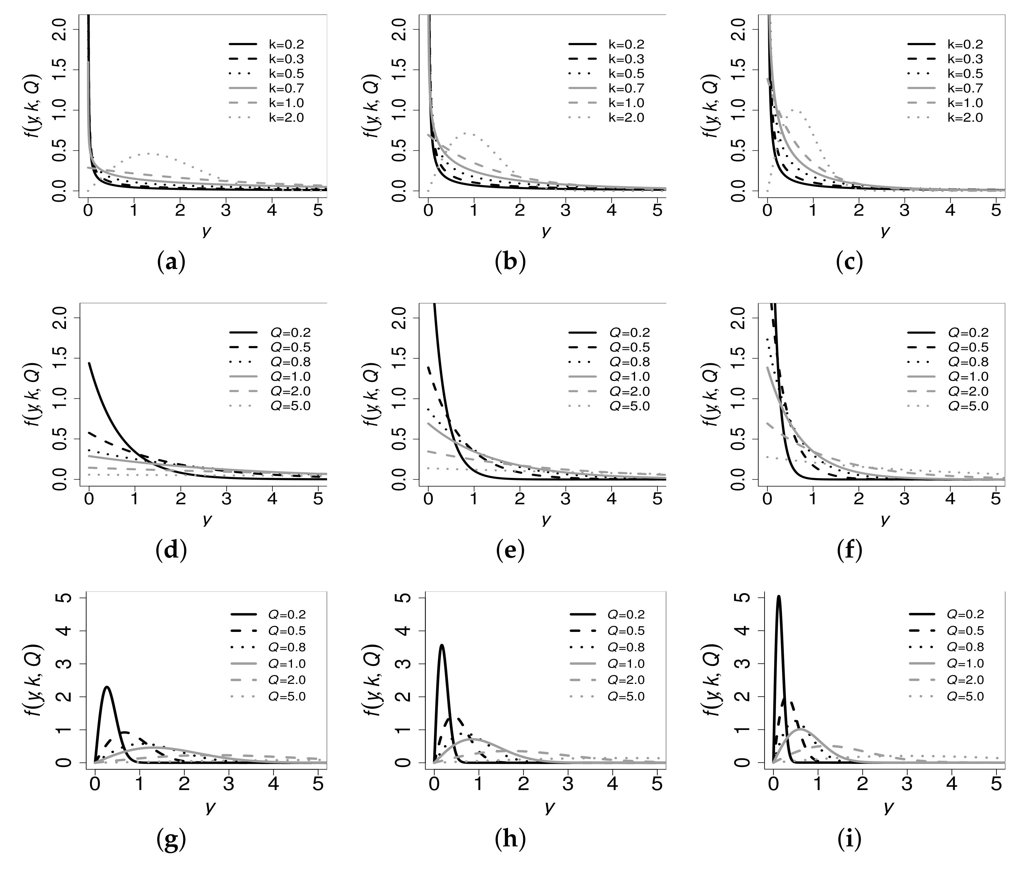
The probability density function of a random variable Y that follows a Weibull distribution with shape and scale parameters k > 0 and λ > 0 , respectively, is given by
f ( y ; λ , k ) = k λ y λ k 1 exp y λ k , y > 0 .
It is possible to prove that, if q ( 0 , 1 ) is a fixed number, the qth quantile of Y corresponds to
Q = λ ( log ( 1 q ) ) 1 / k ,
from which we obtain
λ = Q ( log ( 1 q ) ) 1 / k .
For more details about properties of the Weibull distribution, see [3] (pp. 629–666) and [8]. Replacing the formula stated in (3) for λ in the expression given in (2), we have a new parameterization of the Weibull distribution based on its quantiles, which is denoted by Wei ( Q , k ) , and its probability density and cumulative distribution functions are formulated, respectively, as
f ( y ; Q , k ) = k y k 1 Q k log ( 1 q ) exp y k Q k log ( 1 q ) , y > 0 ,
and
F ( y ; Q , k ) = 1 ( 1 q ) y k Q , y > 0 .

2.2. Shape Analysis

Figure 3 shows the behavior of the reparameterized Weibull probability density function defined in (4) under different values of the parameters. Note that, as Q decreases, the kurtosis of the distribution increases; see Figure 3d–i. Thus, when Q increases, the tails are heavier. Moreover, observe in Figure 3a–c that, when k takes values less or equal to one, the distribution mode is zero, while if it takes values greater than one, this mode is positive.

2.3. The Weibull Quantile Regression Model

Let Y 1 , , Y n be independent random variables with Y i Wei ( Q i , k ) , for i { 1 , , n } . Suppose that the quantile parameter Q i can be modeled by
h ( Q i ) = x i β , i { 1 , , n } ,
where β = ( β 0 , β 1 , , β p 1 ) , for p < n , is a vector of unknown regression parameters and x i = ( 1 , x i 1 , , x i ( p 1 ) ) represents the values of p covariates. Note that the link function h is invertible, at least twice differentiable, and has positive support. The last condition of h guarantees that the quantile is modeled for a positive expression. Link functions that may be considered are, for example, h ( u ) = log k ( u ) and h ( u ) = u a , with a 2 and k being a positive integer number.
Note that the reparametrization of the Weibull distribution by quantiles is necessary to formulate the Weibull quantile regression defined in (6), which allows us to model any quantile value of the distribution. Furthermore, this reparameterization makes it possible to incorporate directly the regression structure given in (6) into the corresponding likelihood function. Note that this structure is different from the traditional quantile regression model with an error component; see [11] (p. 29). Doing that, as mentioned, the distributional assumption is directly related to the response variable, permitting statistical tools based on the associated likelihood function to be obtained in a similar form to GLM.

3. Estimation, Inference and Goodness of Fit

3.1. Parameter Estimation

Let y = ( y 1 , , y n ) be an observation of ( Y 1 , , Y n ) , with Y i Wei ( Q i , k ) , for i { 1 , , n } . The log-likelihood function of the model given in (6) for θ = ( β , k ) based on y can be written as
( θ ) = ( θ ; y ) = i = 1 n i ( Q i , k ) ,
where i ( Q i , k ) stated in (7) is formulated as
i ( Q i , k ) = log ( log ( 1 q ) ) + log ( k ) + ( k 1 ) log ( y i ) k log ( Q i ) + y i k Q i k log ( 1 q ) .
Therefore, the score vector has as components ˙ β j , for j { 0 , 1 , , p 1 } , and ˙ k , expressed as
˙ β j = ( θ ) β j = i = 1 n z i a i x i j , ˙ k = ( θ ) k = i = 1 n b i ,
where
z i = k Q i k Q i k 1 y i k log ( 1 q ) , a i = 1 h ( Q i ) , h ( Q i ) = d h d Q i , b i = log ( y i ) log ( Q i ) + 1 k + y i Q i k log y i Q i log ( 1 q ) .
The elements of the associated Hessian matrix are written as
¨ β l β j = 2 ( θ ) β l β j = i = 1 n c i x i j x i l , ¨ β j k = 2 ( θ ) β j k = i = 1 n m i a i x i j , ¨ k k = 2 ( θ ) k 2 = i = 1 n d i ,
where
c i = k Q i 2 + k ( k + 1 ) Q i k 2 y i k log ( 1 q ) a i 2 z i a i h ( Q i ) ( h ( Q i ) ) 2 , h ( Q i ) = d 2 h d Q i 2 , m i = 1 Q i y i k Q i k 1 log ( 1 q ) 1 k log Q i y i , d i = 1 k 2 + log ( 1 q ) y i Q i k log 2 y i Q i .
To estimate the vector θ of parameters with the maximum likelihood method, we often solve the equation ˙ θ = 0 p + 1 , where 0 p + 1 is the p + 1 null vector. However, no closed-form expressions for the maximum likelihood estimates can be obtained, and therefore numeric procedures must be used to calculate the estimate of θ . For example, the Broyden–Fletcher–Goldfarb–Shanno (BFGS) method or other quasi-Newton algorithms may be considered; see [32]. Different algorithms are implemented in the R software, including the BFGS approach for constrained and unconstrained maximization; see [27].

3.2. Inference and Hypothesis Testing

Under some regularity conditions [14] (pp. 118–119), it is possible to establish that
θ ^ ˙ N p + 1 ( θ , ( I ( θ ) ) 1 ) ,
where I ( θ ) is the expected Fisher information matrix, which may be computed by
I ( θ ) = E 2 ( θ ) θ θ .
We can obtain approximate confidence intervals using the results provided in (10), whereas for approximating the information matrix defined in (11), we may employ the observed Fisher information matrix stated as
J ( θ ) = 2 ( θ ) θ θ ,
whose elements established in (12) may be calculated from (9), evaluated at θ = θ ^ .
Note that if we want to test the hypothesis H 0 : θ = θ 0 versus the alternative hypothesis H 1 : θ θ 0 , where, as mentioned, θ = ( β , k ) , then we can use the Wald and likelihood ratio tests. The Wald [33] and likelihood ratio statistics based on the observed Fisher information matrix [34] are, respectively, given by
W = ( θ ^ θ 0 ) J ( θ ^ ) ( θ ^ θ 0 ) ,
L = 2 ( θ 0 ) ( θ ^ ) .
When n , both statistics converge to a random variable that follows a χ 2 distribution with r degrees of freedom, χ r 2 in short, where r is the number of parameters under H 0 , which is rejected, at a nominal level of significance α , if the statistic computed according to (13) or (14) is greater than χ r , 1 α 2 , which denotes the 100 ( 1 α ) th χ r 2 quantile.

3.3. Residuals

To evaluate the model adequacy—that is, to assess the fit of our model to a data set—we can employ the RQ and GCS residuals. For our reparameterized Weibull model, these residuals are given, respectively, by
r i RQ = Φ 1 F ( y i ; Q ^ i ; k ^ ) , r i GCS = log ( S ( y i ; Q ^ i ; k ^ ) ) ,
where Φ is the standard normal cumulative distribution function; F is given by (5); Q ^ i and k ^ are the maximum likelihood estimates of Q i and k, respectively; and S = 1 F is the corresponding survival function. The RQ residual is approximately standard normal distributed, whereas the GCS residual follows a standard exponential asymptotic distribution when the model is correctly specified, whatever its specification is.

4. Monte Carlo Simulation

4.1. Setting

We present the results of two Monte Carlo simulation studies for the Weibull quantile regression model. The first scenario considers the evaluation of the statistical performance of the maximum likelihood estimators, while the second scenario assesses the empirical distribution of the residuals. Both simulation scenarios consider the following setting: sample size n { 50 , 200 , 600 } , and combinations of the vector of true parameters stated as ( β 0 , β 1 , k ) = ( 0.50 , 1.00 , 0.50 ) , ( β 0 , β 1 , k ) = ( 1.00 , 0.50 , 1.00 ) , ( β 0 , β 1 , k ) = ( 1.00 , 0.50 , 2.00 ) , ( β 0 , β 1 , k ) = ( 2.50 , 1.00 , 0.50 ) , ( β 0 , β 1 , k ) = ( 2.50 , 1.00 , 1.00 ) , ( β 0 , β 1 , k ) = ( 2.50 , 1.00 , 2.00 ) , including different degrees of asymmetry; and q { 0.10 , 0.50 , 0.90 } , with 1000 Monte Carlo replications for each n. The Weibull quantile regression samples are generated using the inverse transformation method applied to the expression formulated in (5), which gives
Y i = log ( 1 U i ) / log ( 1 q ) Q i 1 / k , i { 1 , , n } ,
where Q i and U i defined in (16) are specified as Q i = exp ( β 0 + β 1 x i ) and U i Uniform ( 0 , 1 ) , with x i being the value of a covariate obtained from a standard normal distribution.

4.2. Scenario 1: Maximum Likelihood Estimation

We employ the R software and its maxBFGS function, which implements the BFGS algorithm with constraints for maximization and requires initial values for estimating β = ( β 0 , β 1 ) and k. We utilize the least square estimator of β assuming a usual linear regression and the maximum likelihood estimate of k based on the observations y 1 , , y n without considering covariates. The maximum likelihood estimates are presented in Table 2, Table 3, Table 4, Table 5, Table 6 and Table 7 wherein the empirical mean, bias, variance, root mean squared error (RMSE), CS, and CK are all reported. A look at the results in Table 2, Table 3, Table 4, Table 5, Table 6 and Table 7 allows us to conclude that, in general, as the sample size increases, the bias, variance, and RMSE of the estimators decrease, as expected. Moreover, β ^ 0 , β ^ 1 , and k ^ seem all to be consistent and asymptotically normal distributed. Our study was conducted on a Dell Inspirion 5748 personal computer with an Intel core i7-4510U CPU, 2.00 GHz × 4, and 8 GB of RAM.

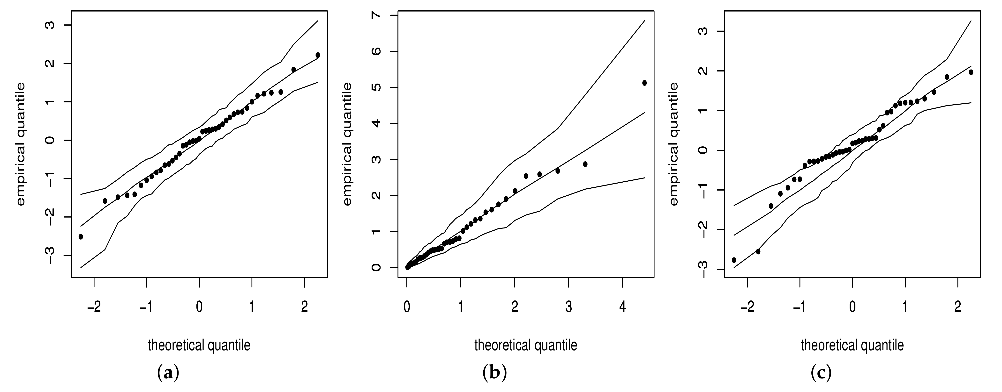
4.3. Scenario 2: Empirical Distribution of the Residuals

Now, we report a second Monte Carlo simulation study to evaluate the performance of the GCS and RQ residuals defined in (15). Table 8 and Table 9 present the empirical mean, SD, CS, and CK for β 0 = 0.5 and β 1 = 1.0 , whose values are expected to be 0, 1, 0, and 3, respectively, for r RQ , and 1, 1, 2, and 9, respectively, for r GCS . From Table 8 and Table 9, we observe that, in general, the considered residuals conform well with the reference distributions. The same conclusions are obtained for the other values of β 0 and β 1 .

5. Local Influence

5.1. Perturbation Matrix and Potentially Influential Cases

Local influence techniques examine the effect of small perturbations in the model data and/or assumptions regarding the estimated parameters. Let ( θ ) be the log-likelihood function for the parameter θ of the model defined by (6), which is named the non-perturbed model. Consider a vector of R n , ω namely, called the vector of perturbation, and we define ( θ ; ω ) as the log-likelihood function of the perturbed model and θ ^ ω as the maximum likelihood estimate of θ obtained from ( θ ; ω ) . Further, let ω 0 R n be a non-perturbation vector such that ( θ ) = ( θ ; ω 0 ) . The likelihood displacement function (LD) defined as
LD ( ω ) = 2 ( θ ^ ) ( θ ^ ω )
is used to detect the impact of ω . We study the local behavior of the surface plot ( ω , LD ( ω ) ) around ω 0 . The direction in which the LD locally changes most rapidly is evaluated; that is, the maximum curvature of the surface. For LD ( ω ) given in (17), the maximum curvature is established as
C max = max d = 1 2 | d B d | ,
where B defined in (18) is given by B = Δ ¨ θ ^ θ ^ Δ and d is a unit-length direction vector; see [22]. The expression ¨ θ ^ θ ^ is the Hessian matrix of ( θ ) evaluated at θ ^ and Δ is a ( p + 1 ) × n perturbation matrix also evaluated at θ = θ ^ and ω = ω 0 . Hence, the elements of Δ are stated as
Δ i j = 2 ( θ ; ω ) θ i ω j θ = θ ^ , ω = ω 0 , i { 0 , 1 , , p } , j { 1 , , n } .
Then, d max is a unit-length eigenvector associated with the maximum absolute eigenvalue of B . The plot of d max versus the index i may be considered to detect whether case i is potentially influential on θ ^ . The direction d = e i , where e i is an n × 1 vector of zeros, with one at the ith position, is another relevant direction to analyze. For such a direction, the normal curvature is C i ( θ ) = 2 | b i i | , where b i i is the ith element of the diagonal of the matrix B . If
C i ( θ ) > 2 i = 1 n C i ( θ ) n = 2 C ¯ ,
then the case i is potentially influential; see [35]. Next, we describe the matrix Δ for different perturbation schemes with its elements defined in generic terms in (19).

5.2. Perturbation Schemes

5.2.1. Case-Weight Perturbation

Consider ω = ( ω 1 , , ω n ) as a weight vector. Then, the perturbed log-likelihood function is defined by ( θ ; ω ) = i = 1 n ω i i ( Q i , k ) , where 0 ω i 1 , for i { 1 , , n } . Therefore, the n columns of Δ are given by
δ i = x i a i z i b i θ = θ ^ , ω = ( 1 , , 1 ) , i { 1 , , n } .

5.2.2. Perturbation on the Response

Now, consider an additive perturbation on the response i by making y i ( ω i ) = y i + ω i s Y , where ω i R and s Y is a scale factor that can be the sample SD of Y, for i { 1 , , n } . Then, the perturbed log-likelihood function corresponds to ( θ ; ω ) = i = 1 n ω i ( Q i , k ) , with
ω i ( Q i , k ) = log ( log ( 1 q ) ) + log ( k ) + ( k 1 ) log ( y i ( ω i ) ) k log ( Q i ) + ( y i ( ω i ) ) k Q i k log ( 1 q ) ,
for i { 1 , , n } . The column vectors of Δ may be expressed as
δ i = x i a i ϕ i ρ i τ i ρ i θ = θ ^ , ω = ( 0 , , 0 ) , i { 1 , , n } ,
where
ϕ i = k 2 Q i k 1 y i k 1 log ( 1 q ) , τ i = 1 y i + y i k 1 Q i k k log y i Q i + 1 log ( 1 q ) , ρ i = s Y .

5.2.3. Perturbation in the Continuous Covariate

Consider an additive perturbation on a particular continuous covariate, x t namely, with t { 1 , , p 1 } , by making x t i ( ω i ) = x t i + ω i s X t , where s X t is, again, a scale factor, which can be taken as the sample SD of X t , and ω i R , for i { 1 , , n } . Therefore, the perturbed log-likelihood function is given by ( θ ; ω ) = i = 1 n ω i ( Q i , k ) , where
ω i ( Q i , k ) = log ( log ( 1 q ) ) + log ( k ) + ( k 1 ) log ( y i ) k log ( Q i ( ω i ) ) + y i k Q i ( ω i ) k log ( 1 q ) ,
with Q i ( ω i ) = h 1 ( x i ( ω i ) β ) and x i ( ω i ) = ( 1 , x i 1 , , x i t ( ω i ) , , x i ( p 1 ) ) , for i { 1 , , n } . Hence, the perturbation matrix takes the form given by
Δ = Δ β Δ k θ = θ ^ , ω = ( 0 , , 0 ) ,
where Δ β = ( Δ β i j ) is a p × n matrix defined as
Δ β i j = s X t β t a i a i x i j z i + s X t β t x i j a i 2 c i , j t , i { 1 , , n } , s X t a i z i + s X t β t a i a i x i t z i + s X t β t x i t a i 2 c i , j = t , i { 1 , , n } ,
with a i being the derivative of a i defined in (8). Here, Δ k = ( ζ 1 , , ζ n ) , with ζ i = s X t β t a i m i .

5.2.4. Perturbation of the Parameter k

In this case, the perturbation scheme consists of changing k by making k i = k / ω i , with ω i > 0 . Then, the perturbed log-likelihood is ( θ ; ω ) = i = 1 n ω i ( Q i , k i ) , where
ω i ( Q i , k i ) = log ( log ( 1 q ) ) + log ( k i ) + ( k i 1 ) log ( y i ) k i log ( Q i ) + y i k i Q i k i log ( 1 q ) , i { 1 , , n } .
The column vectors of Δ can be expressed as
δ i = x i a i ξ i η i θ = θ ^ , ω = ( 1 , , 1 ) , i { 1 , , n } ,
where ξ i = k m i and η i = k d i .

6. Illustrative Example

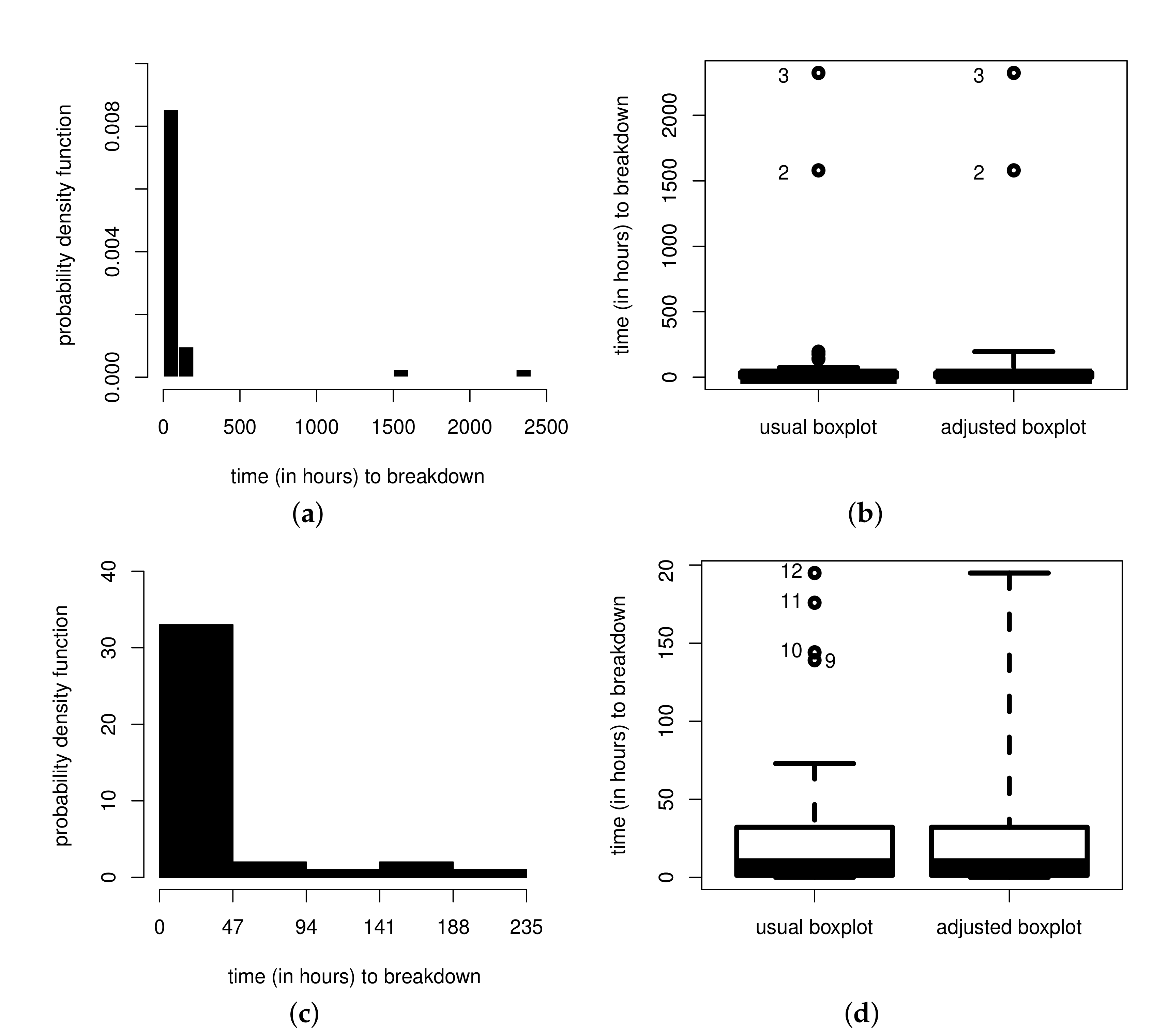
6.1. The Adjusted Weibull Quantile Regression

To illustrate the use of the Weibull quantile regression formulated in this paper, we assume Y i Wei ( Q i , k ) and that our goal is to model the median. Consider two link functions (logarithm and square root) for a systematic component of the regression model, which are respectively stated as
( L 1 ) log ( Q i ) = x i β , ( L 2 ) Q i = x i β ,
for i { 1 , , 41 } , where β = ( β 0 , β 1 ) is the vector of regression coefficients, and x i = ( 1 , x i ) is the vector of values of X i = ( 1 , X i ) .
We implement the function quant.weibull.reg() in the R software, which allows us to fit Weibull quantile regression models to a data set, computing information criteria and residuals. To select the best model amongst a set of options, the AIC, BIC, and CAIC can be used. These information criteria assume the existence of an unknown “true model”. The AIC chooses the model whose divergence in relation to the “true model” is the minimum within the competing models and may be computed by
AIC = 2 ( θ ^ ) + 2 m ,
where ( θ ^ ) is the log-likelihood function evaluated at θ = θ ^ and m is the number of parameters of the proposed model, in our case m = p + 1 . When the number of parameters is large, the AIC can have a deficient behavior. For this reason, a correction to the AIC is proposed as
CAIC = AIC + 2 m ( m + 1 ) n m 1 ,
where n is the sample size. The BIC is another information criterion for model selection based on maximizing the probability of choosing the true model and corresponds to
BIC = 2 ( θ ^ ) + m log ( n ) .
In all these criteria, the best model, among a set of candidates, has the smallest value.
Another measure to be employed to choose among competing models is R M 2 , which works similarly to the usual R 2 measure in mean regression and is defined as
R M 2 = 1 exp 2 n ( θ ˜ ) ( θ ^ ) ,
where ( θ ˜ ) and ( θ ^ ) are the maximized log-likelihood for the regression model without any covariate and with all covariates, respectively.
Values of the AIC, BIC, and CAIC defined in (22), (23), and (24), R M 2 stated in (25) and the corresponding log-likelihood functions are reported in Table 10. We conclude that the model with the logarithm link function (L1) should be used to describe the median.
Now, we compare model L1 with the proposed model in [10]. This comparison is not obvious since the construction of both models is different. Then, we compare both models in terms of R M 2 defined in (25) and the pseudo-R 2 proposed for the Koenker–Bassett model [11] given by
R KB 2 = 1 V 1 ( q ) V 0 ( q ) ,
where V 1 ( q ) is the sum of weighted distances for the full qth quantile regression model and V 0 ( q ) is the sum of weighted distance for the model that includes only an intercept; that is, with no covariates. For our data, using (25) and (26), we obtain R M 2 = 0.71 and R KB 2 = 0.03 , allowing us to conclude that our model is a better option for describing this data set.
Another relevant comparison is to consider a GLM-type model based on the Weibull distribution and reparameterized by its mean. We fit this model to our data taking the logarithmic link function. The value of the mean squared prediction error for the Weibull mean regression is 425,939.8, and for the median regression it is 231,845.7, meaning that, in terms of prediction error, our adjusted quantile model outperforms a GLM-type model based on the Weibull distribution.
Table 11 reports the maximum likelihood estimates for the model parameters, their approximated standard errors (SEs), and p-values based on the Wald test (described in Section 2). Thus, the predictive model is given by log ( Q ^ ) = 20.97 0.56 x , for x > 0 .
We evaluate the distributional assumption of the model by using the RQ and GCS residuals; that is, r i RQ and r i GCS , respectively. The QQ plots with envelopes for these residuals are presented in Figure 4, where all points are inside the bands. Therefore, r i RQ (a) and r i GCS (b) follow approximately standard normal and standard exponential distributions, respectively. This result allows us to validate that the response variable follows a Weibull distribution.
To compare the Weibull quantile regression model with other direct competing models, we adjust the Birnbaum–Saunders quantile regression model [2,16] with logarithm link function, which considers a response variable with an asymmetric distribution. For the Birnbaum–Saunders model with our data, the CAIC, BIC, and R M 2 values are 334.96, 339.45 and 0.67, respectively. Note that the CAIC and BIC values are greater than the corresponding values for model L1; see Table 10. Furthermore, the value of R M 2 is less than for model L1. The CAIC and BIC values are 531.31 and 535.80 for the normal model given in (1). Additionally, the residual r i RQ has been computed for the Birnbaum–Saunders model, and the QQ plot with envelopes is shown in Figure 4c. We observe that, compared with the QQ plot in Figure 4a, the behavior is less homogeneous around a straight line, and there are points outside of the bands. Therefore, by considering the CAIC, BIC, and QQ plots of residuals, we conclude that the Weibull quantile regression outperforms the Birnbaum–Saunders quantile regression as well.

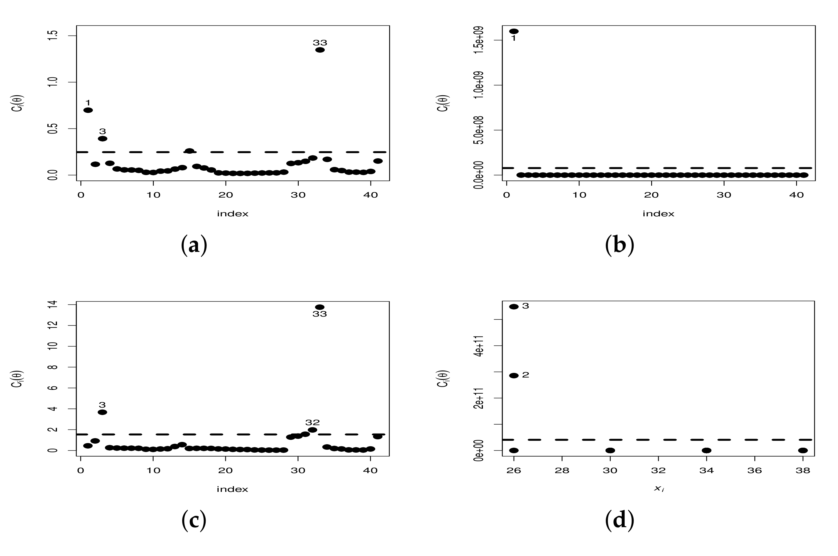
6.2. Local Influence Analysis

Next, we analyze potentially influential cases by their local influence for the Weibull quantile regression with link L1, considering the four perturbation schemes as described in Section 5. In Figure 5, we show the index plots of C i ( θ ) defined in (20) for each of them. Note that five cases are indicated as potentially influential, namely cases #1, #2, #3, #32, and #33. Observe that the local influence technique detects some atypical cases identified previously. From Figure 5d, note that small values for covariate X influence the estimates.
We study the impact on the model inference considering the three cases most repeated in the index plots of Figure 5, which are cases #1, #3, and #33. The sets of cases { # 1 } , { # 3 } , { # 33 } , { # 1 , # 3 } , { # 1 , # 33 } , { # 3 , # 33 } , and { # 1 , # 3 , # 33 } are removed and the model parameters are re-estimated. To determine the variation in the estimates of model parameters and in the associated SEs, we use the value of the relative changes (RCs) for each component of the parameter vector θ ; that is,
RC θ j ( i ) = θ ^ j θ ^ j ( i ) θ ^ j × 100 % , RC SE ( θ ^ j ) ( i ) = SE ^ ( θ ^ j ) SE ^ ( θ ^ j ) ( i ) SE ^ ( θ ^ j ) × 100 % ,
where θ ^ j ( i ) and SE ^ ( θ ^ j ) ( i ) denote the maximum likelihood estimates of θ j and the estimated SE of the associated estimator, respectively, obtained after removing case i, for j { 1 , 2 , 3 } and i { 1 , , 41 } , with θ 1 = β 0 , θ 2 = β 1 , and θ 3 = k .
Table 12 reports the values of RCs for the data of time to electrical breakdown of an insulating fluid and the Weibull quantile regression. Note that the largest values of RCs are obtained when we remove cases #1 and #33, with the highest change occurring in the parameter k. The RCs of all parameters show a change close to 20%. However, we do not find any inferential change. Therefore, our study of local influence measures derived in this paper allows us to detect potentially influential cases, but these do not affect the model inference. Thus, the analysis of local influence presented with the data of the time to electrical breakdown of an insulating fluid permits us to conclude that the Weibull quantile regression model is nonsensitive to the atypical cases detected and exhibits an excellent performance to model this data set.

6.3. Coefficients across Quantiles

Quantile regression gives us a full description of how the covariates can affect the different values of the response variable. To show this, we consider the model given by log ( Q ) = β 0 + β 1 x . If the covariate X increases from x 0 to x 1 = x 0 + 1 , then the value of modeled quantile changes from Q 0 = exp ( β 0 + β 1 x 0 ) to Q 1 = exp β 0 + β 1 ( x 0 + 1 ) , and then we have ( Q 1 Q 0 ) / Q 0 = exp ( β 1 ) 1 . Therefore, the coefficient β 1 is related to the percentage of change in the considered quantile when the covariate increases in one unit; see [36]. To illustrate this, we fit the Weibull regression model formulated in (21) considering the quantiles q { 0.1 , 0.25 , 0.5 , 0.75 , 0.9 } . In addition, we use a procedure to find the optimal value of q, q opt namely, that is, the value of q that maximizes the log-likelihood function. We consider the profile log-likelihood method based on a grid of values of q { 0.01 , 0.02 , , 0.99 } . Then, we estimate the Weibull regression parameters and compute the corresponding log-likelihood function. This procedure has been used in other contexts for Weibull models by [8] (pp. 426–433), where it is called a non-failing algorithm. The results are presented in Table 13. We observe that the covariate has the largest impact on higher levels of the response variable. For example, for values near to the 25th quantile of the response variable, if the voltage increases by 1 kV, the values of the response change by ( exp ( 0.62 ) 1 ) × 100 % = 47 % . If we consider values close to the 90th quantile, it changes by ( exp ( 0.52 ) 1 ) × 100 % = 41 % .

7. Concluding Remarks

This paper has proposed novel quantile regression models for a response variable that follows an asymmetrical behavior based on a new parameterization of the Weibull distribution. We have estimated the new model parameters by using the maximum likelihood method and discussed hypothesis testing based on the Wald and likelihood ratio statistics. In addition, we have used the randomized quantile and generalized Cox–Snell residuals to evaluate the fit of the model. Monte Carlo simulation studies have found that (i) the maximum likelihood estimators are empirically consistent and asymptotically normal distributed (Table 2, Table 3, Table 4, Table 5, Table 6 and Table 7), and (ii) the randomized quantile and generalized Cox–Snell residuals follow a standard normal distribution and exponential distribution with a parameter equal to one, respectively (Table 8 and Table 9). Furthermore, we have derived local influence techniques to analyze the impact of a perturbation on the estimation of model parameters considering four schemes. We have applied the proposed model to a data set related to the time to electrical breakdown of an insulating fluid. The experimental results of this data analysis have shown the excellent performance of the proposed model to the data, making it a better choice than the usual normal regression model and other asymmetrical quantile regression models proposed in the literature. Some observations have been detected as potentially influential cases for our local diagnostic analysis (Figure 5) but without inferential change. Furthermore, we have studied the impact of the covariates on the quantiles of the response.
This work has evidenced that the new proposed model is helpful for independent data and a response variable with positive support. This new quantile regression model can also be suitable for small samples. However, we remark some limitations of our models and the proposed methodology. For example, diverse phenomena frequently provide other types of data to those analyzed in this study, such as censored, functional, spatial, and temporal data, as well as structures of measurement errors, and partial least squares, all of which are suitable to be studied to increase the predictive capability in the modeling; see [37,38,39,40,41]. Then, it is necessary to formulate new models based on our approach to study these phenomena in such types of data and modeling structures. These structures are not an easy aspect to be explored, especially with spatially correlated data, because new multivariate distributions based on asymmetrical models need to be proposed and parameterized in terms of quantiles; see [38]. Furthermore, our proposal allows likelihood methods to be used, and thus this proposal can be applied to different distributions for modeling data, but adaptations of the corresponding methodology for each of these distributions must be performed.
An idea to enhance the empirical analysis of our proposal involves the following steps. First, consider the covariate with the highest simple correlation coefficient. Second, estimate the slope and intercept parameters in h ( Q ) . Third, taking a quantile as the median, create a data set on y and x stating a table with the observed values of y, the fitted values of y, and the residuals as their difference. Fourth, plot the observed and fitted values against the x values to allow the assessment of the model. In addition, least squares-fitted values can be displayed in the same graphical plot. A one-at-a-time cross-validation separates one observation for prediction from the remaining data, which adds a simple aspect about prediction that is also valuable. Other aspects related to k-fold cross validation are also appealing. Additionally, the relationship between a quantile and the covariates by means of a link function must be evaluated in each case, since it may not be correctly specified, implying extra analyses to achieve a better modeling. Moreover, measures such as the Cook distance and generalized leverage are essential diagnostic aspects of all statistical modeling, and they must be further studied for the newly proposed model. Weibull-type distributions with an extreme value index are widely used in many areas such as environmental sciences, hydrology, and meteorology; see [42]. Our proposed methodology can be adapted to this type of distributions. These and other aspects are part of our ongoing research.

Author Contributions

Data curation, L.S., H.S. and C.M.; investigation, L.S., V.L. and H.S.; formal analysis and methodology, L.S., V.L., H.S., C.M. and J.M.S.; writing—original draft, L.S., H.S. and C.M.; writing—review and editing, V.L. and J.M.S. All authors have read and agreed to the submitted version of the manuscript.

Funding

The research was partially funded by FONDECYT, project grant numbers 1200525 (V. Leiva and L. Sánchez) and 11190636 (C. Marchant) from the National Agency for Research and Development (ANID) of the Chilean government under the Ministry of Science, Technology, Knowledge, and Innovation; and by ANID-Millennium Science Initiative Program–NCN17_059 (C. Marchant).

Institutional Review Board Statement

Not applicable.

Informed Consent Statement

Not applicable.

Data Availability Statement

The analyzed data and used codes are available under request.

Acknowledgments

The authors would also like to thank the Editor and three reviewers for their constructive comments which led to the improvement of the presentation of the manuscript.

Conflicts of Interest

The authors declare no conflict of interest.

References

  1. Ventura, M.; Saulo, H.; Leiva, V.; Monsueto, S. Log-symmetric regression models: Information criteria, application to movie business and industry data with economic implications. Appl. Stoch. Model. Bus. Ind. 2019, 35, 963–977. [Google Scholar] [CrossRef]
  2. Mazucheli, J.; Leiva, V.; Alves, B.; Menezes, A.F.B. A new quantile regression for modeling bounded data under a unit Birnbaum–Saunders distribution with applications in medicine and politics. Symmetry 2021, 13, 682. [Google Scholar] [CrossRef]
  3. Johnson, N.; Kotz, S.; Balakrishnan, N. Continuous Univariate Distributions; Wiley: New York, NY, USA, 1994. [Google Scholar]
  4. Castillo, E.; Hadi, A.S.; Balakrishnan, N.; Sarabia, J.M. Extreme Value and Related Models with Applications in Engineering and Science; Wiley: Hoboken, NJ, USA, 2005. [Google Scholar]
  5. Saraiva, E.F.; Suzuki, A.K. Bayesian computational methods for estimation of two-parameters Weibull distribution in presence of right-censored data. Chilean J. Stat. 2017, 8, 25–43. [Google Scholar]
  6. Weibull, W. A statistical distribution of wide applicability. J. Appl. Mech. 1951, 18, 293–297. [Google Scholar] [CrossRef]
  7. Arnold, B.C.; Castillo, E.; Sarabia, J.M. Modeling the fatigue life of longitudinal elements. Nav. Res. Logist. Q. 1996, 43, 885–895. [Google Scholar] [CrossRef]
  8. Rinne, H. The Weibull Distribution; Chapman and Hall: London, UK, 2009. [Google Scholar]
  9. Laplace, P. Theorie Analytique des Probabilites; Editions Jacques Gabayr: Paris, France, 1818. [Google Scholar]
  10. Koenker, R.; Bassett, G. Regression quantiles. Econometrica 1978, 46, 33–50. [Google Scholar] [CrossRef]
  11. Hao, L.; Naiman, D.Q. Quantile Regression. Sage Publications: Thousand Oaks, CA, USA, 2007. [Google Scholar]
  12. Davino, C.; Furno, M.; Vistocco, D. Quantile Regression: Theory and Applications; Wiley: London, UK, 2013. [Google Scholar]
  13. Koenker, R.; Chernozhukov, V.; He, X.; Peng, L. Handbook of Quantile Regression; CRC Press: Boca Raton, FL, USA, 2018. [Google Scholar]
  14. Davison, A. Statistical Models; Cambridge University Press: Cambrigde, UK, 2003. [Google Scholar]
  15. McCullagh, P.; Nelder, J.A. Generalized Linear Models; Chapman and Hall: London, UK, 1983. [Google Scholar]
  16. Sánchez, L.; Leiva, V.; Galea, M.; Saulo, H. Birnbaum-Saunders quantile regression and its diagnostics with application to economic data. Appl. Stoch. Model. Bus. Ind. 2021, 37, 53–73. [Google Scholar] [CrossRef]
  17. Saulo, H.; Dasilva, A.; Leiva, V.; Sánchez, L.; de la Fuente-Mella, H. Log-symmetric quantile regression models. Stat. Neerl. 2021, in press. [Google Scholar] [CrossRef]
  18. Cook, R.D.; Weisberg, S. Residuals and Influence in Regression; Chapman and Hall: London, UK, 1982. [Google Scholar]
  19. Maddala, G.S. Limited-Dependent and Qualitative Variables in Econometrics; Cambridge University Press: Cambridge, UK, 1983. [Google Scholar]
  20. Dunn, P.; Smyth, G. Randomized quantile residuals. J. Comput. Graph. Stat. 1996, 5, 236–244. [Google Scholar]
  21. Saulo, H.; Leão, J.; Leiva, V.; Aykroyd, R.G. Birnbaum-Saunders autoregressive conditional duration models applied to high-frequency financial data. Stat. Pap. 2019, 60, 1605–1629. [Google Scholar] [CrossRef] [Green Version]
  22. Cook, R.D. Assessment of local influence. J. R. Stat. Soc. B 1986, 48, 133–169. [Google Scholar] [CrossRef]
  23. Santos-Neto, M.; Cysneiros, F.J.A.; Leiva, V.; Barros, M. Reparameterized Birnbaum-Saunders regression models with varying precision. Electron. J. Stat. 2016, 10, 2825–2855. [Google Scholar] [CrossRef]
  24. Garcia-Papani, F.; Leiva, V.; Uribe-Opazo, M.A.; Aykroyd, R.G. Birnbaum-Saunders spatial regression models: Diagnostics and application to chemical data. Chemom. Intell. Lab. Syst. 2018, 177, 114–128. [Google Scholar] [CrossRef] [Green Version]
  25. Leiva, V.; Sanchez, L.; Galea, M.; Saulo, H. Global and local diagnostic analytics for a geostatistical model based on a new approach to quantile regression. Stoch. Environ. Res. Risk Assess. 2020, 34, 1457–1471. [Google Scholar] [CrossRef]
  26. Meeker, W.; Escobar, L. Statistical Methods for Reliability Data; Wiley: New York, NY, USA, 1998. [Google Scholar]
  27. R Core Team. R: A Language and Environment for Statistical Computing; R Foundation for Statistical Computing: Vienna, Austria, 2020. [Google Scholar]
  28. Therneau, T. A Package for Survival Analysis in R; R Package Version 3.2-10. 2021. Available online: https://CRAN.R-project.org/package=survival (accessed on 18 October 2021).
  29. Maechler, M.; Rousseeuw, P.; Croux, C.; Todorov, V.; Ruckstuhl, A.; Salibian-Barrera, M.; Verbeke, T.; Koller, M.; Conceicao, E.L.; di Palma, M.A. Package ‘robustbase’. Basic Robust Statistics. 2021. Available online: https://cran.r-project.org/web/packages/robustbase/robustbase.pdf (accessed on 18 October 2021).
  30. Noufaily, A.; Jones, M. Parametric quantile regression based on the generalized gamma distribution. J. R. Stat. Soc. C 2013, 62, 723–740. [Google Scholar] [CrossRef]
  31. Mazucheli, J.; Menezes, A.; Fernandes, L.; Puziol, R.; Ghitany, M. The unit-Weibull distribution as an alternative to the Kumaraswamy distribution for the modeling of quantiles conditional on covariates. J. Appl. Stat. 2019, 47, 954–974. [Google Scholar] [CrossRef]
  32. Nocedal, J.; Wright, S. Numerical Optimization; Springer: New York, NY, USA, 2006. [Google Scholar]
  33. Wald, A. Sequential Analysis; Wiley: New York, NY, USA, 1947. [Google Scholar]
  34. Wilks, S.S. The large-sample distribution of the likelihood ratio for testing composite hypotheses. Ann. Math. Stat. 1938, 9, 60–62. [Google Scholar] [CrossRef]
  35. Lesaffre, E.; Verbeke, G. Local influence in linear mixed models. Biometrics 1998, 54, 570–582. [Google Scholar] [CrossRef]
  36. Weisberg, S. Applied Linear Regression; Wiley: New York, NY, USA, 2014. [Google Scholar]
  37. Huerta, M.; Leiva, V.; Liu, S.; Rodriguez, M.; Villegas, D. On a partial least squares regression model for asymmetric data with a chemical application in mining. Chemom. Intell. Lab. Syst. 2019, 190, 55–68. [Google Scholar] [CrossRef]
  38. Sánchez, L.; Leiva, V.; Galea, M.; Saulo, H. Birnbaum-Saunders quantile regression models with application to spatial data. Mathematics 2020, 8, 1000. [Google Scholar] [CrossRef]
  39. Calle-Saldarriaga, A.; Laniado, H.; Zuluaga, F.; Leiva, V. Homogeneity tests for functional data based on depth-depth plots with chemical applications. Chemom. Intell. Lab. Syst. 2021, in press. [Google Scholar] [CrossRef]
  40. Leiva, V.; Saulo, H.; Souza, R.; Aykroyd, R.G.; Vila, R. A new BISARMA time series model for forecasting mortality using weather and particulate matter data. J. Forecast. 2021, 40, 346–364. [Google Scholar] [CrossRef]
  41. Figueroa-Zúñiga, J.I.; Bayes, C.L.; Leiva, V.; Liu, S. Robust Beta Regression Modeling with Errors-in-Variables: A Bayesian Approach and Numerical Applications. Stat. Pap. 2022, in press. [Google Scholar] [CrossRef]
  42. He, F.; Wang, H.J.; Tong, T. Extremal linear quantile regression with Weibull-type tails. Stat. Sin. 2020, 30, 1357–1377. [Google Scholar] [CrossRef]
Figure 1. Histogram (a) and boxplots (b) for the data of times to electrical breakdown with the full data set, and histogram (c) and boxplots (d) for the data set without cases #2 and #3.
Mathematics 09 02768 g001
Figure 2. QQ plot with envelopes of the Pearson residual for normal regression with the data of times to electrical breakdown.
Mathematics 09 02768 g002
Figure 3. Plots of the Wei ( Q , k ) probability density function for q = 0.25 (left), q = 0.5 (center) and q = 0.75 (right), with Q = 1.0 (ac), k = 1.0 (df) and k = 2.0 (gi).
Mathematics 09 02768 g003
Figure 4. QQ plot with envelope of r i RQ (a) and r i CGS (b) for the Weibull median regression and of r i RQ for the Birnbaum–Saunders quantile regression model with logarithm link (c), using the data of the time to electrical breakdown of an insulating fluid.
Mathematics 09 02768 g004
Figure 5. Index plots of C i ( θ ) under case-weight perturbation (a), response perturbation (b), perturbation of the parameter k (c), and covariate perturbation X (d) for the data of time to electrical breakdown of an insulating fluid and the Weibull quantile regression.
Mathematics 09 02768 g005
Table 1. Descriptive statistics for the data of times to electrical breakdown (in hours).
MedianMeanSDCVCSCK y ( 1 ) y ( n ) n
7.7400122.51430.243.514.3620.930.092323.7041
Table 2. Statistics from simulated Weibull regression data ( q = 0.10 , β 0 = 0.50 , β 1 = 1.00 ).
k = 0.5 k = 1.00 k = 2.00
Statistic n = 50 n = 200 n = 600 n = 50 n = 200 n = 600 n = 50 n = 200 n = 600
β ^ 0 β ^ 0 β ^ 0
True value0.50000.50000.5000 0.50000.50000.5000 0.50000.50000.5000
Mean0.60110.54910.5138 0.55060.52440.5069 0.52530.51220.5034
Bias0.10110.04910.0138 0.05060.02440.0069 0.02530.01220.0034
Variance0.67470.17460.0537 0.16870.04370.0134 0.04220.01090.0034
RMSE0.82760.42070.2322 0.41380.21040.1161 0.20690.10520.0581
CS−0.1288−0.1332−0.1183 −0.1287−0.1331−0.1179 −0.1286−0.1327−0.1180
CK3.14813.01242.9364 3.14753.01052.9359 3.14763.00942.9360
β ^ 1 β ^ 1 β ^ 1
True value1.00001.00001.0000 1.00001.00001.0000 1.00001.00001.0000
Mean1.01930.98310.9954 1.00970.99150.9977 1.00480.99580.9988
Bias0.0193−0.0169−0.0046 0.0097−0.0085−0.0023 0.0048−0.0042−0.0012
Variance0.89660.23560.0745 0.22410.05890.0186 0.05600.01470.0047
RMSE0.94710.48560.2730 0.47350.24280.1365 0.23680.12140.0682
CS0.0619−0.03440.1067 0.0621−0.03470.1068 0.0621−0.03480.1067
CK2.84433.06063.0311 2.84543.06073.0311 2.84403.06333.0311
k ^ k ^ k ^
True value0.50000.50000.5000 1.00001.00001.0000 2.00002.00002.0000
Mean0.52100.50610.5021 1.04191.01221.0043 2.08382.02442.0086
Bias0.02100.00610.0021 0.04190.01220.0043 0.08380.02440.0086
Variance0.00360.00080.0003 0.01440.00330.0010 0.05760.01300.0041
RMSE0.06360.02920.0162 0.12710.05840.0324 0.25430.11680.0648
CS0.58240.24460.0840 0.58260.24500.0840 0.58310.24470.0841
CK3.75672.92772.6255 3.75632.92472.6253 3.75772.92462.6250
Table 3. Statistics from simulated Weibull regression data ( q = 0.50 , β 0 = 0.50 , β 1 = 1.00 ).
k = 0.5 k = 1.00 k = 2.00
Statistic n = 50 n = 200 n = 600 n = 50 n = 200 n = 600 n = 50 n = 200 n = 600
β ^ 0 β ^ 0 β ^ 0
True value0.50000.50000.5000 0.50000.50000.5000 0.50000.50000.5000
Mean0.49630.51520.5015 0.49820.50760.5008 0.49910.50380.5004
Bias−0.00370.01520.0015 −0.00180.00760.0008 −0.00090.00380.0004
Variance0.34230.08850.0261 0.08560.02210.0065 0.02140.00550.0016
RMSE0.58510.29780.1615 0.29250.14890.0808 0.14630.07450.0404
CS−0.2084−0.1717−0.1039 −0.2085−0.1716−0.1039 −0.2084−0.1715−0.1038
CK3.00763.13212.9602 3.00783.13202.9601 3.00753.13192.9600
β ^ 1 β ^ 1 β ^ 1
True value1.00001.00001.0000 1.00001.00001.0000 1.00001.00001.0000
Mean1.01940.98310.9954 1.00970.99160.9977 1.00490.99580.9988
Bias0.0194−0.0169−0.0046 0.0097−0.0084−0.0023 0.0049−0.0042−0.0012
Variance0.89650.23550.0745 0.22410.05890.0186 0.05600.01470.0047
RMSE0.94700.48560.2730 0.47350.24280.1365 0.23680.12140.0683
CS0.0619−0.03430.1067 0.0619−0.03430.1068 0.0620−0.03440.1067
CK2.84473.06123.0311 2.84483.06123.0309 2.84503.06093.0310
k ^ k ^ k ^
True value0.50000.50000.5000 1.00001.00001.0000 2.00002.00002.0000
Mean0.52100.50610.5021 1.04191.01221.0043 2.08382.02432.0086
Bias0.02100.00610.0021 0.04190.01220.0043 0.08380.02430.0086
Variance0.00360.00080.0003 0.01440.00330.0010 0.05760.01300.0041
RMSE0.06360.02920.0162 0.12710.05840.0324 0.25430.11680.0648
CS0.58260.24480.0841 0.58250.24480.0840 0.58240.24480.0840
CK3.75682.92562.6256 3.75652.92562.6254 3.75592.92562.6255
Table 4. Statistics from simulated Weibull regression data ( q = 0.90 , β 0 = 0.50 , β 1 = 1.00 ).
k = 0.5 k = 1.00 k = 2.00
Statistic n = 50 n = 200 n = 600 n = 50 n = 200 n = 600 n = 50 n = 200 n = 600
β ^ 0 β ^ 0 β ^ 0
True value0.50000.50000.5000 0.50000.50000.5000 0.50000.50000.5000
Mean0.42950.49390.4937 0.46480.49690.4969 0.48240.49850.4984
Bias−0.0705−0.0061−0.0063 −0.0352−0.0031−0.0031 −0.0176−0.0015−0.0016
Variance0.30750.07940.0235 0.07690.01980.0059 0.01920.00500.0015
RMSE0.55900.28180.1534 0.27950.14090.0767 0.13970.07040.0384
CS−0.1501−0.1109−0.1234 −0.1505−0.1108−0.1234 −0.1504−0.1109−0.1234
CK2.92053.15072.9856 2.91913.15042.9857 2.91903.15042.9857
β ^ 1 β ^ 1 β ^ 1
True value1.00001.00001.0000 1.00001.00001.0000 1.00001.00001.0000
Mean1.01940.98310.9953 1.00970.99150.9977 1.00480.99580.9988
Bias0.0194−0.0169−0.0047 0.0097−0.0085−0.0023 0.0048−0.0042−0.0012
Variance0.89650.23550.0745 0.22410.05890.0186 0.05600.01470.0047
RMSE0.94700.48560.2730 0.47350.24280.1365 0.23680.12140.0682
CS0.0617−0.03430.1067 0.0620−0.03430.1067 0.0619−0.03420.1067
CK2.84533.06123.0310 2.84483.06123.0311 2.84473.06093.0311
k ^ k ^ k ^
True value0.50000.50000.5000 1.00001.00001.0000 2.00002.00002.0000
Mean0.52100.50610.5021 1.04191.01221.0043 2.08382.02432.0086
Bias0.02100.00610.0021 0.04190.01220.0043 0.08380.02430.0086
Variance0.00360.00080.0003 0.01440.00330.0010 0.05760.01300.0041
RMSE0.06360.02920.0162 0.12710.05840.0324 0.25430.11680.0648
CS0.58250.24480.0840 0.58250.24490.0840 0.58250.24470.0840
CK3.75672.92572.6254 3.75672.92582.6255 3.75662.92572.6254
Table 5. Statistics from simulated Weibull regression data ( q = 0.10 , β 0 = 1.00 , β 1 = 2.50 ).
k = 0.5 k = 1.00 k = 2.00
Statistic n = 50 n = 200 n = 600 n = 50 n = 200 n = 600 n = 50 n = 200 n = 600
β ^ 0 β ^ 0 β ^ 0
True value1.00001.00001.0000 1.00001.00001.0000 1.00001.00001.0000
Mean1.10131.04931.0138 1.05061.02441.0069 1.02531.01221.0034
Bias0.10130.04930.0138 0.05060.02440.0069 0.02530.01220.0034
Variance0.67470.17470.0537 0.16870.04370.0134 0.04220.01090.0034
RMSE0.82760.42080.2322 0.41380.21040.1161 0.20690.10520.0581
CS−0.1295−0.1353−0.1183 −0.1290−0.1330−0.1180 −0.1292−0.1332−0.1185
CK3.14893.01342.9364 3.14803.01042.9358 3.14853.01162.9364
β ^ 1 β ^ 1 β ^ 1
True value2.50002.50002.5000 2.50002.50002.5000 2.50002.50002.5000
Mean2.51932.48302.4954 2.50972.49152.4977 2.50482.49582.4989
Bias0.0193−0.0170−0.0046 0.0097−0.0085−0.0023 0.0048−0.0042−0.0011
Variance0.89620.23580.0745 0.22410.05890.0186 0.05600.01470.0047
RMSE0.94690.48590.2730 0.47350.24280.13657 0.23680.12140.0682
CS0.0622−0.03760.1068 0.0619−0.03460.1066 0.0621−0.03360.1070
CK2.84543.06853.0310 2.84473.06173.0290 2.84523.06083.0310
k ^ k ^ k ^
True value0.50000.50000.5000 1.00001.00001.0000 2.00002.00002.0000
Mean0.52100.50610.5021 1.04191.01221.0043 2.08382.02432.0086
Bias0.02100.00610.0021 0.04190.01220.0043 0.08380.02430.0086
Variance0.00360.00080.0003 0.01440.00330.0010 0.05760.01300.0041
RMSE0.06360.02920.0162 0.12710.05840.0324 0.25430.11680.0648
CS0.58240.24610.0840 0.58260.24530.0829 0.58240.24560.0836
CK3.75742.92652.6256 3.75712.92722.6223 3.75632.92612.6256
Table 6. Statistics from simulated Weibull regression data ( q = 0.50 , β 0 = 1.00 , β 1 = 2.50 ).
k = 0.5 k = 1.00 k = 2.00
Statistic n = 50 n = 200 n = 600 n = 50 n = 200 n = 600 n = 50 n = 200 n = 600
β ^ 0 β ^ 0 β ^ 0
True value1.00001.00001.0000 1.00001.00001.0000 1.00001.00001.0000
Mean0.99631.01521.0015 0.99821.00761.0008 0.99911.00381.0004
Bias−0.00370.01520.0015 −0.00180.00760.0008 −0.00090.00380.0004
Variance0.34230.08850.0261 0.08560.02210.0065 0.02140.00550.0016
RMSE0.58510.29780.1615 0.29250.14890.0807 0.14630.07450.0404
CS−0.2084−0.1718−0.1039 −0.2083−0.1716−0.1038 −0.2084−0.1715−0.1044
CK3.00763.13242.9603 3.00733.13232.9601 3.00693.13122.9588
β ^ 1 β ^ 1 β ^ 1
True value2.50002.50002.5000 2.50002.50002.5000 2.50002.50002.5000
Mean2.51942.48312.4954 2.50972.49162.4977 2.50492.49582.4989
Bias0.0194−0.0169−0.0046 0.0097−0.0084−0.0023 0.0049−0.0042−0.0011
Variance0.89640.23550.0745 0.22410.05890.0186 0.05600.01470.0047
RMSE0.94700.48560.2730 0.47350.24280.1365 0.23680.12140.0682
CS0.0619−0.03430.1067 0.0618−0.03430.1066 0.0618−0.03420.1060
CK2.84473.06123.0310 2.84483.06153.0307 2.84533.06003.0309
k ^ k ^ k ^
True value0.50000.50000.5000 1.00001.00001.0000 2.00002.00002.0000
Mean0.52100.50610.5021 1.04191.01221.0043 2.08382.02432.0087
Bias0.02100.00610.0021 0.04190.01220.0043 0.08380.02430.0087
Variance0.00360.00080.0003 0.01440.00330.0010 0.05760.01300.0041
RMSE0.06360.02920.0162 0.12710.05840.0324 0.25430.11680.0648
CS0.58250.24470.0838 0.58240.24460.0838 0.58250.24460.0820
CK3.75652.92552.6254 3.75632.92572.6253 3.75712.92552.6247
Table 7. Statistics from simulated Weibull regression data ( q = 0.90 , β 0 = 1.00 , β 1 = 2.50 ).
k = 0.5 k = 1.00 k = 2.00
Statistic n = 50 n = 200 n = 600 n = 50 n = 200 n = 600 n = 50 n = 200 n = 600
β ^ 0 β ^ 0 β ^ 0
True value1.00001.00001.0000 1.00001.00001.0000 1.00001.00001.0000
Mean0.92950.99380.9937 0.96480.99690.9969 0.98240.99850.9984
Bias−0.0705−0.0062−0.0063 −0.0352−0.0031−0.0031 −0.0176−0.0015−0.0016
Variance0.30740.07940.0235 0.07690.01980.0059 0.01920.00500.0015
RMSE0.55890.28180.1534 0.27950.14090.0767 0.13970.07050.0384
CS−0.1500−0.1104−0.1234 −0.1505−0.1111−0.1234 −0.1504−0.1107−0.1230
CK2.91993.15142.9857 2.91903.15132.9857 2.91903.15012.9853
β ^ 1 β ^ 1 β ^ 1
True value2.50002.50002.5000 2.50002.50002.5000 2.50002.50002.5000
Mean2.51942.48322.4954 2.50972.49162.4977 2.50482.49582.4988
Bias0.0194−0.0168−0.0046 0.0097−0.0084−0.0023 0.0048−0.0042−0.0012
Variance0.89630.23550.0745 0.22410.05890.0186 0.05600.01470.0047
RMSE0.94690.48560.2730 0.47350.24280.1365 0.23680.12140.0683
CS0.0615−0.03490.1067 0.0620−0.03430.1068 0.0619−0.03410.1064
CK2.84543.06173.0310 2.84483.06103.0311 2.84483.06093.0310
k ^ k ^ k ^
True value0.50000.50000.5000 1.00001.00001.0000 2.00002.00002.0000
Mean0.52100.50610.5021 1.04191.01221.0043 2.08382.02432.0086
Bias0.02100.00610.0021 0.04190.01220.0043 0.08380.02430.0086
Variance0.00360.00080.0003 0.01440.00330.0010 0.05760.01300.0041
RMSE0.06360.02920.0162 0.12710.05840.0324 0.25430.11680.0648
CS0.58250.24480.0840 0.58250.24490.0840 0.58250.24480.0838
CK3.75662.92552.6255 3.75672.92572.6254 3.75662.92562.6257
Table 8. Summary statistics of the GCS residuals ( β 0 = 0.5 ; β 1 = 1.0 ).
Statistic k = 0.50 k = 1.00 k = 2.00
n = 50 n = 200 n = 600 n = 50 n = 200 n = 600 n = 50 n = 200 n = 600
q = 0.10
Mean1.00001.00001.0000 1.00001.00001.0000 1.00001.00001.0000
SD0.98820.99630.9986 0.98820.99630.9986 0.98820.99630.9986
CS1.57111.85251.9394 1.57101.85241.9394 1.57111.85241.9394
CK5.71867.65848.3894 5.71857.65788.3894 5.71877.65808.3895
q = 0.50
Mean1.00001.00001.0000 1.00001.00001.0000 1.00001.00001.0000
SD0.98820.99630.9986 0.98820.99630.9986 0.98820.99630.9986
CS1.57111.85241.9394 1.57111.85241.9394 1.57111.85241.9394
CK5.71897.65778.3894 5.71887.65778.3895 5.71887.65778.3895
q = 0.90
Mean1.00001.00001.0000 1.00001.00001.0000 1.00001.00001.0000
SD0.98820.99630.9986 0.98820.99630.9986 0.98820.99630.9986
CS1.57111.85241.9394 1.57111.85241.9394 1.57111.85241.9394
CK5.71897.65778.3895 5.71887.65778.3895 5.71897.65778.3895
Table 9. Summary statistics of the RQ residuals ( β 0 = 0.5 ; β 1 = 1.0 ).
Statistic k = 0.50 k = 1.00 k = 2.00
n = 50 n = 200 n = 600 n = 50 n = 200 n = 600 n = 50 n = 200 n = 600
q = 0.10
Mean0.00120.00040.0001 0.00120.00040.0001 0.00120.00040.0001
SD1.01341.00331.0011 1.01341.00331.0011 1.01331.00331.0011
CS0.01420.00260.0009 0.01420.00270.0009 0.01420.00270.0009
CK2.74872.92582.9774 2.74862.92582.9774 2.74872.92582.9774
q = 0.50
Mean0.00120.00030.0001 0.00120.00040.0001 0.00120.00030.0001
SD1.01341.00331.0011 1.01341.00331.0011 1.01341.00331.0011
CS0.01420.00270.0009 0.01420.00270.0009 0.01420.00270.0009
CK2.74872.92582.9774 2.74872.92582.9774 2.74872.92582.9774
q = 0.90
Mean0.00120.00040.0001 0.00120.00030.0001 0.00120.00030.0001
SD1.01341.00331.0011 1.01341.00331.0011 1.01341.00331.0011
CS0.01420.00270.0009 0.01420.00270.0009 0.01420.00270.0009
CK2.74872.92582.9774 2.74872.92582.9774 2.74872.92582.9774
Table 10. Values of AIC, BIC, CAIC, and log-likelihood function for Weibull median-regression models with the data of time to electrical breakdown of an insulating fluid.
ModelAICCAICBIC R M 2 Log-Likelihood
L1327.07327.71332.210.71−160.53
L2351.63352.28356.770.47−172.81
Table 11. Estimate, SE, and p-value of the indicated parameter for the data of time to electrical breakdown of an insulating fluid.
Statistic β 0 ^ β 1 ^ k ^
Estimate20.97−0.560.82
SE1.860.060.10
p-value<0.01<0.01<0.01
Table 12. RCs of maximum likelihood estimates and of the associated estimated SEs for the indicated cases, and respective p-values for the data of time to electrical breakdown of an insulating fluid and the Weibull quantile regression.
Parameter
Removed Case(s) β 0 β 1 k
NoneRC( θ ^ )N/AN/AN/A
RC( SE ^ )N/AN/AN/A
p-value<0.01<0.01<0.01
{ # 1 } RC( θ ^ )3.413.415.81
RC( SE ^ )2.522.785.38
p-value<0.01<0.01<0.01
{ # 3 } RC( θ ^ )4.875.230.77
RC( SE ^ )18.8618.310.14
p-value<0.01<0.01<0.01
{ # 33 } RC( θ ^ )1.461.988.16
RC( SE ^ )13.2313.2612.43
p-value<0.01<0.01<0.01
{ # 1 , # 3 } RC( θ ^ )0.450.714.74
RC( SE ^ )12.2511.375.15
p-value<0.01<0.01<0.01
{ # 1 , # 33 } RC( θ ^ )4.464.9215.72
RC( SE ^ )15.2115.5020.27
p-value<0.01<0.01<0.01
{ # 3 , # 33 } RC( θ ^ )3.283.117.54
RC( SE ^ )3.654.1112.51
p-value<0.01<0.01<0.01
{ # 1 , # 3 , # 33 } RC( θ ^ )0.560.7614.77
RC( SE ^ )5.406.1920.12
p-value<0.01<0.01<0.01
Table 13. Estimates of the parameters of the Weibull quantile regression model considering different quantiles, with insulating fluid data.
Estimate q = 0.10 q = 0.25 q = 0.50 q = 0.75 q = 0.90 q opt = 0.32
β 0 ^ 18.9721.8020.9720.1921.0220.50
β 1 ^ −0.57−0.62−0.56−0.52−0.52−0.57
k ^ 0.840.810.820.840.840.85
Publisher’s Note: MDPI stays neutral with regard to jurisdictional claims in published maps and institutional affiliations.

