Set Stability and Set Stabilization of Boolean Control Networks Avoiding Undesirable Set

Abstract

The traditional set stability of Boolean networks (BNs) refers to whether all the states can converge to a given state subset. Different from the existing results, the set stability investigated in this paper is whether all states in a given initial set can converge to a given destination set. This paper studies the set stability and set stabilization avoiding undesirable sets of BNs and Boolean control networks (BCNs), respectively. First, by virtue of the semi-tensor product (STP) of matrices, the dynamics of BNs avoiding a given undesirable set are established. Then, the set reachability and set stability of BNs from the initial set to destination set avoiding an undesirable set are investigated, respectively. Furthermore, the set stabilization of BCNs from the initial set to destination set avoiding a given undesirable set are investigated. Finally, a design method for finding the time optimal set stabilizer is proposed, and an example is provided to illustrate the effectiveness of the results.

1. Introduction

A Boolean network (BN) was first proposed by Kauffman, which laid the foundation for the study of gene regulation networks [1]. Since then, BNs have been widely investigated by researchers from biology, physics, and many other fields [2,3,4,5].

Two basic issues, stability and stabilization have been studied extensively [6,7,8,9], where the limit behavior of BNs is considered. For example, stable functions of BNs are studied in [6]. The stability of equilibria states and limit cycles in sparsely connected BNs is investigated by [7]. However, it is difficult to find all the limit cycles and fixed points for general BNs before the emergence of semi-tensor products (STP) of matrices.

STP is a new matrix product that overcomes the constraint of dimension in traditional matrix product [10,11]. All the limit cycles and fixed points of general BNs are revealed by using STP [12]. In addition, controllability [13,14], observability [15,16], optimal control [17], perturbation [18,19], and other properties [20,21,22,23,24,25,26] have also been investigated. It can be seen that STP is becoming an effective tool for studying BNs.

This paper investigates the set stability and set stabilization of Boolean control networks (BCNs) avoiding a given undesirable set. The motivations for investigating set stability and set stabilization come from two aspects.

(a) Practical problems:  In some cases, the research interest focuses on whether a subset of state space of an interconnected subsystem converges to or can be stabilized to another subset, which is termed set stability from the initial set to destination set in this paper. A typical example of set stability is the partial synchronization of a collection of locally interconnected systems [27]. The other example is the finite-time consensus of finite field networks with a probabilistic time delay, which can be converted into the set stability from the state space to destination set [28].

(b) Hotspot of recent research:  Set stability and set stabilization have been a research hotspot recently. Professor Guo [29] investigated the set stability and set stabilization of BCNs based on invariant subsets. The set stabilization of multivalued logical systems was studied in [30]. However, the existing results on set stability and set stabilization are from the full state space to a given state subset. Different from the existing results, the set stability and set stabilization problem studied in this paper are from the initial state set to the destination state set, which is the generation of traditional set stability and set stabilization.

Another concern that frequently occurs in biological systems is to prevent certain states of genes from being in an unfavorable or dangerous environment [31]. For example, in the treatment of diseases, some states of the genes or cell may cause new diseases, and they should be avoided [32]. In BCNs, such a situation is called state or input constrained. There are some works that focus on BCNs with state or input constraints. The reachability and controllability of BCNs under certain constraints were investigated in [33]. Professor Guo [34] studied the observability of BCNs with input constraints. The set controllability of logical control networks with state constraints was considered in [35]. Therefore, it is crucial to consider state constraints when studying the set stability and set stabilization of BCNs.

This paper investigates the set stability and set stabilization of BCNs with state constraints in the framework of STP. The contributions of this paper are as follows.

(i)

The dynamics of BNs and BCNs avoiding given undesirable set is established using STP.

(ii)

The set reachability and set stability of BNs and BCNs from the initial set to destination set are provided avoiding a given undesirable set, respectively. The criteria are provided with matrix forms, which are easily verified.

(iii)

The calculation formula of the transition period from each state of an initial set to a given destination set is given. The algorithm of a time optimal stabilizer is designed.

The organization of the rest of this paper is as follows: In Section 2, some preliminaries and symbol explanations of STP of matrices are provided. In Section 3, the definition of set stability of BNs avoiding undesirable states is first provided. Then, a discrete-time dynamic system is constructed, based on which the necessary and sufficient condition of set stability avoiding an undesirable set is obtained. In Section 4, the problem of the set stabilization of BCNs avoiding undesirable sets is discussed. In Section 5, a design method for finding the time optimal set stabilizer is proposed, and an example is provided to illustrate the effectiveness of the results. A brief conclusion is given in Section 6.

2. Preliminaries

In this section, we first list some notations:

(1)

${\mathcal{M}}_{m\times n}$ is the set of all $m\times n$ real matrices; ${\mathbb{R}}^n$ is the set of n-dimensional real vectors.

(2)

${\mathrm{Col}}_i\left(M\right)\left({\mathrm{Row}}_i\left(M\right)\right)$ is the i-th column (row) of matrix M; $\mathrm{Col}\left(M\right)\left(\mathrm{Row}\left(M\right)\right)$ is the set of columns (rows) of matrix M.

(3)

${\delta }_n^i$ is the i-th column of n-dimensional identity matrix $I_n$.

(4)

$\mathcal{D}:=\{0,1\}$.

(5)

${\Delta }_n=\mathrm{Col}\left(I_n\right)$, $\Delta :={\Delta }_2$.

(6)

Assume $L=[{\delta }_m^{i_1}{\delta }_m^{i_2}\dots {\delta }_m^{i_n}]$, and then its shorthand form is $L={\delta }_m[i_1{i}_2\dots i_n]$.

(7)

${\mathbf{1}}_r$(${\mathbf{0}}_r$) represents the column vector of length r whose all terms are 1(0).

(8)

Let $A\in {\mathcal{M}}_{m\times n}$, A is called a logical matrix if $\mathrm{Col}\left(A\right)\subseteq {\Delta }_m$.

(9)

Denote by ${\mathcal{L}}_{m\times n}$ the set of $m\times n$ dimension logical matrices.

(10)

Let $A\in {\mathcal{M}}_{m\times n}$, ${\left(A\right)}_{i,j}$ denotes the $(i,j)$-element of matrix A.

(11)

$A=\left(a_{ij}\right)$ is called a Boolean matrix if $a_{ij}\in \mathcal{D}$, and denote by ${\mathcal{B}}_{m\times n}$ the set of $m\times n$ dimension Boolean matrices.

(12)

The following is the definition of Boolean addition of Boolean matrices

$$\begin{array}{c}\hfill \begin{array}{c}\left\{\begin{array}{c}\alpha {+}_{\mathcal{B}}\beta :=\alpha \vee \beta ,\forall \alpha ,\beta \in \mathcal{D}\hfill \\ {}_{\left(\mathcal{B}\right)}\sum _{i=1}^n{\alpha }_i:={\alpha }_1\vee {\alpha }_2\vee \dots {\alpha }_n,\forall {\alpha }_i\in \mathcal{D}\hfill \\ X{+}_{\mathcal{B}}Y=\left(x_{ij}{+}_{\mathcal{B}}{y}_{ij}\right)\in {\mathcal{B}}_{m\times n},\forall X,Y\in {\mathcal{B}}_{m\times n}.\hfill \end{array}\right.\hfill \end{array}\end{array}$$

(13)

For any $X\in {\mathcal{B}}_{m\times n}$, $Y\in {\mathcal{B}}_{n\times p}$, $X{\times }_{\mathcal{B}}Y:=Z={\left(z_{ij}\right)}_{m\times p}$ is called the Boolean product of X and Y, where $z_{ij}{=}_{\left(\mathcal{B}\right)}{\sum }_{k=1}^n{x}_{ik}\wedge y_{kj}\in \mathcal{D}$.

(14)

If $X\in {\mathcal{B}}_{n\times n}$, then $X^{\left(k\right)}:=\underset{k}{\underbrace{\left(X{\times }_{\mathcal{B}}X{\times }_{\mathcal{B}}\dots {\times }_{\mathcal{B}}X\right)}}$.

(15)

Let $X,Y\in {\mathbb{R}}^n$, then $X>Y$ represents ${\left(X\right)}_{i,1}>{\left(Y\right)}_{i,1},\forall i\in \{1,2,\dots ,n\}$.

(16)

Assume that $X=\left(x_{ij}\right)\in {\mathcal{B}}_{m\times n}$, $Y=\left(y_{ij}\right)\in {\mathcal{L}}_{m\times n}$. Then, $X\wedge Y=(x_{ij}\wedge y_{ij})\in {\mathcal{L}}_{m\times n}$.

(17)

For any $\mathbf{F}\in {\mathcal{B}}_{m\times n}$, the logical sub-matrix of $\mathbf{F}$ is defined as $F\in {\mathcal{L}}_{m\times n}$, if $F\wedge \mathbf{F}=F$. Let $\phi \left(\mathbf{F}\right)$ denotes the set of all logical sub-matrix of $\mathbf{F}$, that is, $\phi \left(\mathbf{F}\right):=\{F\in {\mathcal{L}}_{m\times n}|F\wedge \mathbf{F}=F\}$. In particular, for any nonzero vector $x\in {\mathcal{B}}_{m\times 1}$, $\phi \left(x\right)=\{z\in {\Delta }_m|z\wedge x=z\}$. For convenience, define ${\phi }^T\left(x\right):=\phi \left(x^T\right)$ for any $x\in {\mathcal{B}}_{1\times n}$.

Definition 1

(Ref. [11]). The STP of two matrices $A\in {\mathcal{M}}_{m\times n}$ and $B\in {\mathcal{M}}_{p\times t}$ is defined as

$$A⋉B=(A\otimes I_{\frac{\alpha }{n}})(B\otimes I_{\frac{\alpha }{p}}),$$

where $\alpha =lcm(n,p)$ is the least common multiple of n and p, and ⊗ is the Kronecker product.

Remark 1.

The STP is a generalization of the ordinary matrix product, thus, we can simply call it “product” and omit the symbol “⋉” without confusion.

Proposition 1

(Ref. [11]). Let $X\in {\mathbb{R}}^t$ and $A\in {\mathcal{M}}_{m\times n}$. Then,

$$XA=(I_t\otimes A)X.$$

Definition 2

(Ref. [11]). Define a matrix $W_{[m,n]}\in {\mathcal{M}}_{mn\times mn}$ as follows

$$W_{[m,n]}:=[{\delta }_n^1\otimes {\delta }_m^1,\dots ,{\delta }_n^n\otimes {\delta }_m^1,{\delta }_n^1\otimes {\delta }_m^2,\dots ,{\delta }_n^n\otimes {\delta }_m^2,\dots ,{\delta }_n^1\otimes {\delta }_m^m,\dots ,{\delta }_n^n\otimes {\delta }_m^m],$$

where $W_{[m,n]}$ is called the swap matrix.

Proposition 2

(Ref.  [11]). Let $X\in {\mathbb{R}}^m$ and $Y\in {\mathbb{R}}^n$ be two column vectors. Then,

$$W_{[m,n]}XY=YX.$$

A function $f:{\mathcal{D}}^n\to \mathcal{D}$ is called a Boolean function. To use matrix expression we identify $0\sim {\delta }_2^1$ and $1\sim {\delta }_2^2$, then $\Delta \sim \mathcal{D}$. Denote $x\left(t\right)={⋉}_{i=1}^n{x}_i\left(t\right)$, where $x_i\left(t\right)\in \Delta$, we have the following proposition:

Proposition 3

(Ref.  [11]). Let $f:{\Delta }^n\to \Delta$ be a logical function. Then, there exists a unique matrix $M_f\in {\mathcal{M}}_{2^n\times 2}$, such that

$$\begin{array}{c}\hfill f(x_1,\cdots ,x_n)=M_f{⋉}_{i=1}^n{x}_i,x_i\in \Delta ,\end{array}$$

where $M_f$ is called the structure matrix of f.

3. Set Stability Avoiding Undesirable Set

In this section, we consider the stability of BN from the initial set to destination set avoiding undesirable set.

3.1. Algebraic Expression of Bn under Restricted State Set

A Markov-type BN with n nodes is described as [11]

$$\begin{array}{c}\hfill \begin{array}{c}\left\{\begin{array}{c}{x}_1(t+1)=f_1(x_1\left(t\right),\cdots ,x_n\left(t\right)),\hfill \\ x_2(t+1)=f_2(x_1\left(t\right),\cdots ,x_n\left(t\right)),\hfill \\ ⋮\hfill \\ x_n(t+1)=f_n(x_1\left(t\right),\cdots ,x_n\left(t\right)),\hfill \end{array}\right.\hfill \end{array}\end{array}$$

(1)

where $x_i\in \mathcal{D}$, $i=1,\cdots ,n$ are state variables; $f_i:{\mathcal{D}}^n\to \mathcal{D}$, $i=1,\cdots ,n$ are Boolean functions.

By virtue of Proposition 3, we obtain its algebraic expression as follows:

$$x(t+1)=Lx\left(t\right),$$

where $x\left(t\right)={⋉}_{i=1}^n{x}_i\left(t\right)$, and $L\in {\mathcal{L}}_{2^n\times 2^n}$ is called the structure matrix of (1).

Consider BN (1) and suppose the undesirable set $\Omega$ is

$$\Omega =\{{\delta }_{2^n}^{k_1},\dots ,{\delta }_{2^n}^{k_{\gamma }}\}\subseteq {\Delta }_{2^n}.$$

Define the initial set $S_0$ and the destination set $S_d$ as follows

$$\begin{array}{c}\hfill \begin{array}{ccc}{S}_0& :=& \left\{{\delta }_{2^n}^{i_1},{\delta }_{2^n}^{i_2},\cdots ,{\delta }_{2^n}^{i_{\alpha }}\right\}\subseteq {\Delta }_{2^n}\backslash \Omega ,\hfill \\ S_d& :=& \left\{{\delta }_{2^n}^{j_1},{\delta }_{2^n}^{j_2},\cdots ,{\delta }_{2^n}^{j_{\beta }}\right\}\subseteq {\Delta }_{2^n}\backslash \Omega .\hfill \end{array}\end{array}$$

(2)

For simplicity, assume

$$i_1<i_2<\cdots <i_{\alpha },j_1<j_2<\cdots <j_{\beta }.$$

Using the initial set and destination set, we give the definition of set stability avoiding undesirable set $\Omega$ of BN (1).

Definition 3.

Consider BN (1) with the initial set $S_0$ and the destination set $S_d$. BN (1) is said to be set stable from $S_0$ to $S_d$ avoiding Ω, if, for any initial state $x_0\in S_0$, there exists a positive integer $T\left(x_0\right)>0$ such that

$$x(t,x_0)\in S_d,\forall t⩾T\left(x_0\right),$$

(3)

and

$$x(k,x_0)\notin \Omega ,k=0,1,2,\dots .$$

(4)

Let $T_{min}\left(x_0\right)$ represent the smallest integer such that (3) and (4) hold, which is called the transient period from $x_0\in S_0$ to $S_d$ avoiding $\Omega$. The transient period of BN (1) is defined as $T_S:={\max }_{x_0\in S_0}{T}_{min}\left(x_0\right)$.

In the following, we give the algebraic expression of BN (1) under restricted state set ${\Delta }_{2^n}\backslash \Omega$ by constructing a matrix $I_{\Omega }$.

Define a Boolean matrix $I_{\Omega }\in {\mathcal{B}}_{2^n\times 2^n}$ related to $\Omega$ as follows

$$\begin{array}{c}\hfill \begin{array}{c}{\mathrm{Col}}_i\left(I_{\Omega }\right)=\left\{\begin{array}{c}{\mathbf{0}}_{2^n},{\delta }_{2^n}^i\in \Omega ,\hfill \\ {\mathrm{Col}}_i\left(I_{2^n}\right),{\delta }_{2^n}^i\notin \Omega .\hfill \end{array}\right.\end{array}\end{array}$$

(5)

Denote by

$$L_{\Omega }=I_{\Omega }L{I}_{\Omega }.$$

According to $L_{\Omega }$, we know that, for the initial state $x\left(0\right)\notin \Omega$, if $x\left(1\right)=L_{\Omega }x\left(0\right)={\mathbf{0}}_{2^n}$, then state $x\left(0\right)$ evolves to $\Omega$ at the first step. We can construct the algebraic expression of BN (1) under restricted state set ${\Delta }_{2^n}\backslash \Omega$ as

$$\mathcal{X}(t+1)=L_{\Omega }\mathcal{X}\left(t\right),$$

(6)

where $\mathcal{X}\left(t\right)\in {\mathcal{B}}_{2^n\times 1}$ is the state that belongs to $({\Delta }_{2^n}\backslash \Omega )\cup \left\{{\mathbf{0}}_{2^n}\right\}$.

Using Equation (6), we can obtain

$$\begin{array}{cc}\hfill \mathcal{X}\left(t\right)=& L_{\Omega }\mathcal{X}(t-1)\hfill \\ \hfill =& L_{\Omega }⋉L_{\Omega }\mathcal{X}(t-2)\hfill \\ \hfill =& \dots \hfill \\ \hfill =& L_{\Omega }^t\mathcal{X}\left(0\right),\hfill \end{array}$$

(7)

where $\mathcal{X}\left(0\right)=x\left(0\right)$. Assume $x\left(0\right)\notin \Omega$. $\mathcal{X}\left(t\right)={\mathbf{0}}_{2^n}$ indicates that state $x\left(0\right)$ will evolve to $\Omega$ within t steps. If $\mathcal{X}\left(t\right)\ne {\mathbf{0}}_{2^n}$, this indicates that the state $x\left(0\right)$ can stay away from $\Omega$ at the first t steps.

3.2. Reachability Avoiding States Set

Theorem 1.

Consider BN (1). The state ${\delta }_{2^n}^i$ is reachable from state ${\delta }_{2^n}^j$ at s-th step while avoiding Ω, if and only if ${\left(L_{\Omega }^s\right)}_{i,j}=1$.

Proof of Theorem 1. 

Note that the state of BN (1) at time t can be expressed as $x(t,x_0)=L^t{x}_0$. According to Definition 3, we know that BN (1) is reachable from ${\delta }_{2^n}^j$ to ${\delta }_{2^n}^i$ while avoiding $\Omega$ at s-th step, if and only if,

$$\begin{array}{c}\hfill \left\{\begin{array}{c}{L}^s{\delta }_{2^n}^j={\delta }_{2^n}^i,\hfill \\ L^k{\delta }_{2^n}^j\notin \Omega ,\forall k=0,1,2,\dots s.\hfill \end{array}\right.\end{array}$$

(8)

It follows from the construction of $L_{\Omega }$ that Equation (8) is equivalent to

$$L_{\Omega }^s{\delta }_{2^n}^j={\delta }_{2^n}^i,$$

which is further equivalent to

$${\left({\delta }_{2^n}^i\right)}^T{L}_{\Omega }^s{\delta }_{2^n}^j=1,$$

that is, ${\left(L_{\Omega }^s\right)}_{i,j}=1$.    □

Remark 2.

On the basis of algebraic Equation (7), Theorem 1 proposes a necessary and sufficient condition to detect the reachability between two states while avoiding Ω. This is prepared for the Proof of Theorem 2.

In the following, we consider the set reachability of BN (1) avoiding undesirable set. According to (2), define matrix $J_0\in {\mathcal{L}}_{2^n\times \alpha }$ related to $S_0$ and the index vector $J_d\in {\mathbb{R}}^{2^n}$ related to $S_d$ as follows, respectively,

$$\begin{array}{c}\hfill \begin{array}{c}{J}_0={\delta }_{2^n}[i_1{i}_2\cdots i_{\alpha }],{\left(J_d\right)}_{i,1}=\left\{\begin{array}{c}1,{\delta }_{2^n}^i\in S_d,\hfill \\ 0,{\delta }_{2^n}^i\notin S_d.\hfill \end{array}\right.\end{array}\end{array}$$

(9)

Theorem 2.

Consider BN (1) with the initial set $S_0$ and destination set $S_d$ as defined by (2).

(1)

BN (1) is reachable from ${\delta }_{2^n}^j\in S_0$ to $S_d$ avoiding Ω, if and only if, there exists an integer $s_j$, such that

$$\begin{array}{c}\hfill J_d^T{L}_{\Omega }^{s_j}{\delta }_{2^n}^j>0.\end{array}$$

(10)

(2)

BN (1) is reachable from $S_0$ to $S_d$ avoiding Ω, if and only if, there exists an integer s, such that

$$\begin{array}{c}\hfill J_d^T\left(\sum _{k=1}^s{L}_{\Omega }^k\right)J_0>{\mathbf{0}}_{\alpha }^T,\end{array}$$

(11)

where $\alpha =|S_0|$ is the cardinality of $S_0$.

Proof of Theorem 2. 

(1) According to Theorem 1, we know that BN (1) is reachable from ${\delta }_{2^n}^j\in S_0$ to $S_d$ avoiding $\Omega$, if and only if there exists an integer $s_j$ such that ${\left(L_{\Omega }^{s_j}\right)}_{r,j}=1$, where ${\delta }_{2^n}^r\in S_d$. That is to say,

$$L_{\Omega }^{s_j}{\delta }_{2^n}^j={\delta }_{2^n}^r\in S_d.$$

(12)

From the construction of $J_d$, we have

$$J_d={}_{\left(\mathcal{B}\right)}\sum _{i=1}^{\beta }{\delta }_{2^n}^{j_i},$$

then Equation (12) holds if and only if

$$J_d^T{L}_{\Omega }^{s_j}{\delta }_{2^n}^j=1>0,$$

which is equivalent to (10).

(2) We know that $x_0\in S_0$ can reach $S_d$ avoiding $\Omega$ if and only if conclusion (10) holds. Denoted by $s_j$ the integer that makes conclusion (10) hold when the initial state $x_0={\delta }_{2^n}^j\in S_0$. Let $s=\max \{s_{i_1},s_{i_2},\dots ,s_{i_{\alpha }}\}$, then BN (1) is reachable from $S_0$ to $S_d$ avoiding $\Omega$ if and only if conclusion (11) can be obtained.    □

Remark 3.

By definition of matrix $J_0$ and the index vector $J_d$, Theorem 2 gives a method to verify whether the given initial state set $S_0$ can reach the destination set $S_d$ while avoiding set Ω. It is noted that all the calculations involved are matrix operations, which are easy to validate by mathematical software.

The following corollary is obvious.

Corollary 1.

(1) BN (1) is reachable from ${\delta }_{2^n}^j\in S_0$ to $S_d$ avoiding Ω, if and only if,

$$J_d^T\sum _{k=1}^{2^n}{\left(L_{\Omega }\right)}^k{\delta }_{2^n}^j>0.$$

(2) 

BN (1) is reachable from $S_0$ to $S_d$ avoiding Ω, if and only if,

$$J_d^T\sum _{k=1}^{2^n}{\left(L_{\Omega }\right)}^k{J}_0>{\mathbf{0}}_{\alpha }^T.$$

3.3. Set Stability Avoiding States Set

In the following, we consider the set stability problem of a BN avoiding $\Omega$ using the largest invariant subset.

Definition 4

(Ref. [29]). A subset $\mathcal{S}\subseteq {\Delta }_{2^n}$ is called an invariant subset of BN (1) if, for any state $x_0\in \mathcal{S}$, $x(t,x_0)\in \mathcal{S},\forall t⩾0$.

The union of all the invariant subsets contained in $S_d$ is the largest invariant subset of $S_d$.

Lemma 1

(Ref. [29]). Consider a state subset $S_d\subseteq {\Delta }_{2^n}$ of BN (1) with $|S_d|=\beta$. Define a matrix $M_d\in {\mathcal{B}}_{2^n\times 2^n}$ related to $S_d$ as follows

$$\begin{array}{c}\hfill \begin{array}{c}{\mathrm{Col}}_i\left(M_d\right)=\left\{\begin{array}{c}{\delta }_{2^n}^i,{\delta }_{2^n}^i\in S_d,\hfill \\ {\mathbf{0}}_{2^n},{\delta }_{2^n}^i\notin S_d.\hfill \end{array}\right.\end{array}\end{array}$$

(13)

Then, the largest invariant subset, denoted by $I\left(S_d\right)$, contained in $S_d$ is

$$I\left(S_d\right)=\mathrm{Col}\left(Q_{S_d}\right)\backslash \left\{{\mathbf{0}}_{2^n}\right\},$$

where

$$Q_{S_d}={\left(M_{d}L\right)}^{\beta }{M}_d.$$

(14)

Using (9) and (14), we can define a vector, called the set stability vector avoiding $\Omega$, as

$$\begin{array}{c}\hfill H:=J_d^T{\times }_{\mathcal{B}}{Q}_{S_d}{\times }_{\mathcal{B}}{L}_{\Omega }^{2^n}{\times }_{\mathcal{B}}{J}_0.\end{array}$$

Remark 4.

According to the properties of the largest invariant set $I\left(S_d\right)$, we know that, for any state $x_0\in I\left(S_d\right)$, it holds that $x(t,x_0)\in I\left(S_d\right),\forall t\ge 0$, and $I\left(S_d\right)\subseteq S_d$. Therefore, the stability from the initial set $S_0$ to destination set $S_d$ is equivalent to the reachability from the initial set $S_0$ to the largest invariant set $I\left(S_d\right)$.

Theorem 3.

Consider BN (1) with the initial set $S_0$ and destination set $S_d$ as defined by (2).

(1) 

BN (1) is set stable from ${\delta }_{2^n}^{i_j}\in S_0$ to $S_d$ avoiding Ω, if and only if,

$$\begin{array}{c}\hfill {\mathrm{Col}}_j\left(H\right)=1.\end{array}$$

(15)

(2) 

BN (1) is set stable from $S_0$ to $S_d$ avoiding Ω, if and only if,

$$\begin{array}{c}\hfill H={\mathbf{1}}_{\alpha }^T.\end{array}$$

(16)

(3) 

If BN (1) is set stable from $S_0$ to $S_d$ avoiding Ω, then for any ${\delta }_{2^n}^{i_j}\in S_0$, we have

$$T_{min}\left({\delta }_{2^n}^{i_j}\right)=\min \left\{\tau \right|J_d^T{Q}_{S_d}{L}_{\Omega }^{\tau }{\delta }_{2^n}^{i_j}=1\}.$$

Proof of Theorem 3. 

(1) Note that ${\left(J_d^T{Q}_{S_d}\right)}^T$ is the index vector related to $I\left(S_d\right)$. According to Theorem 2, we know that BN (1) is reachable from ${\delta }_{2^n}^{i_j}\in S_0$ to $I\left(S_d\right)$ avoiding $\Omega$, if and only if, there exists an integer $s_{i_j}$, such that

$$\begin{array}{c}\hfill \left(J_d^T{Q}_{S_d}\right)L_{\Omega }^{s_{i_j}}{\delta }_{2^n}^{i_j}=1>0.\end{array}$$

(17)

Combining the properties of the largest invariant set $I\left(S_d\right)$, we can find that Equation (17) holds if and only if BN (1) is stable from ${\delta }_{2^n}^{i_j}\in S_0$ to $I\left(S_d\right)$ avoiding $\Omega$.

In addition, since system (1) has $2^n$ finite states, then it is easy to obtain from (17) that

$$\begin{array}{c}\hfill J_d^T{Q}_{S_d}{L}_{\Omega }^{2^n}{\delta }_{2^n}^{i_j}=1>0,\end{array}$$

that is,

$$\begin{array}{cc}\hfill {\mathrm{Col}}_j\left(H\right)& =J_d^T{Q}_{S_d}{L}_{\Omega }^{2^n}{J}_0{\delta }_{2^n}^{i_j}\hfill \\ \hfill & =J_d^T{Q}_{S_d}{L}_{\Omega }^{2^n}{\delta }_{2^n}^{i_j}\hfill \\ \hfill & =1.\hfill \end{array}$$

(2) BN (1) is set stable from $S_0$ to $S_d$ avoiding $\Omega$, if and only if it is stable from $x_0$ to $S_d$ avoiding $\Omega$ for any $x_0\in S_0$. That is, ${\mathrm{Col}}_j\left(H\right)=1$ for any $j=1,2,\dots ,\alpha$. The result is proven.

(3) If BN (1) is set stable from $S_0$ to $S_d$ avoiding $\Omega$, then, for any ${\delta }_{2^n}^{i_j}\in S_0$, we have ${\mathrm{Col}}_j\left(H\right)=1$. That is to say, there exists a smallest integer $\tau$ such that

$$\begin{array}{cc}\hfill J_d^T{Q}_{S_d}{L}_{\Omega }^{\tau }{\delta }_{2^n}^{i_j}& =J_d^T{Q}_{S_d}{L}_{\Omega }^{\tau }{J}_0{\delta }_{2^n}^{i_j}\hfill \\ \hfill & =H{\delta }_{2^n}^{i_j}\hfill \\ \hfill & ={\mathrm{Col}}_j\left(H\right)\hfill \\ \hfill & =1.\hfill \end{array}$$

Combining to the definition of transient period, it is easy to verify that

$$T_{min}\left({\delta }_{2^n}^{i_j}\right)=\min \left\{\tau \right|J_d^T{Q}_{S_d}{L}_{\Omega }^{\tau }{\delta }_{2^n}^{i_j}=1\},\forall {\delta }_{2^n}^{i_j}\in S_0.$$

   □

Remark 5.

Theorem 3 not only presents the criteria of set stability of BNs from the initial set $S_0$ to destination $S_d$, but also gives the method to calculate the transition period of any given state from $S_0$ to set $S_d$. In addition, the criteria are provided in vector form to facilitate verification.

Example 1.

Consider the Drosophila melanogaster segmentation polarity gene network

$$\begin{array}{c}\hfill \left\{\begin{array}{c}{x}_1(t+1)=x_1\left(t\right)\wedge \neg x_2\left(t\right)\wedge \neg x_4\left(t\right),\hfill \\ x_2(t+1)=\neg x_1\left(t\right)\wedge x_2\left(t\right)\wedge \neg x_3\left(t\right),\hfill \\ x_3(t+1)=x_1\left(t\right)\vee x_3\left(t\right),\hfill \\ x_4(t+1)=x_2\left(t\right)\vee x_4\left(t\right),\hfill \\ x_5(t+1)=\left(\neg x_2\left(t\right)\wedge \neg x_4\left(t\right)\right)\vee \left(x_5\left(t\right)\wedge \neg x_1\left(t\right)\wedge \neg x_3\left(t\right)\right),\hfill \\ x_6(t+1)=\left(\neg x_1\left(t\right)\wedge \neg x_3\left(t\right)\right)\vee \left(x_6\left(t\right)\wedge \neg x_2\left(t\right)\wedge \neg x_4\left(t\right)\right),\hfill \end{array}\right.\end{array}$$

(18)

where $x_1,x_2,x_3,x_4$ represent four different secreted proteins wingless, and $x_5$ and $x_6$ represent two different transmembrane receptor proteins patched. Please refer to  [32] and [26] for their specific meanings.

Let $x\left(t\right)={⋉}_{i=1}^6{x}_i\left(t\right)$. Then, the algebraic form of (18) can be obtained as follows

$$x(t+1)=Lx\left(t\right),$$

where

$$\begin{array}{cc}\hfill L={\delta }_{64}& [5252525252525252\hfill \\ & 5252525252525252\hfill \\ \hfill & 5252525221222122\hfill \\ & 5252525221222122\hfill \\ \hfill & 5252525252525252\hfill \\ & 4141434341414343\hfill \\ \hfill & 5252525253545354\hfill \\ & 5757595961616161].\hfill \end{array}$$

Suppose

$$\begin{array}{cc}\hfill S_0=& \{{\delta }_{64}^{13},{\delta }_{64}^{20},{\delta }_{64}^{44},{\delta }_{64}^{47},{\delta }_{64}^{51},{\delta }_{64}^{60}\},\hfill \\ \hfill S_d=& \{{\delta }_{64}^{23},{\delta }_{64}^{43},{\delta }_{64}^{52},{\delta }_{64}^{59},{\delta }_{64}^{62}\},\hfill \end{array}$$

and the undesirable set

$$\Omega =\{{\delta }_{64}^{29},{\delta }_{64}^{42},{\delta }_{64}^{48}\}.$$

First, according to (9) and (13), we have

$$\begin{array}{cc}\hfill J_0& ={\delta }_{64}\left[132044475160\right],\hfill \\ \hfill J_d& =[0000000000000000\hfill \\ \hfill & 0000100000000000\hfill \\ \hfill & 0000000000100000\hfill \\ \hfill & 0001000000100100],\hfill \end{array}$$

and

$$\begin{array}{cc}\hfill M_d={\delta }_{64}[& 0000000000000000\hfill \\ \hfill & 00002300000000000\hfill \\ \hfill & 00000000004300000\hfill \\ \hfill & 0005200000059006200],\hfill \end{array}$$

where ${\delta }_{64}^0$ is a zero column vector with dimension 64.

By Lemma 1, we obtain

$$\begin{array}{cc}\hfill Q_{S_d}& ={\left(M_{d}L\right)}^5{M}_d\hfill \\ \hfill & ={\delta }_{64}[0000000000000000\hfill \\ \hfill & 0000000000000000\hfill \\ \hfill & 00000000004300000\hfill \\ \hfill & 000520000005900000].\hfill \end{array}$$

Then, the largest invariant subset of $S_d$ is obtained as follows

$$I\left(S_d\right)=\{{\delta }_{64}^{43},{\delta }_{64}^{52},{\delta }_{64}^{59}\}.$$

Next, according to the undesirable set $\Omega$, $L_{\Omega }$ can be obtained as

$$\begin{array}{cc}\hfill L_{\Omega }={\delta }_{64}& [5252525252525252\hfill \\ & 5252525252525252\hfill \\ \hfill & 5252525221222122\hfill \\ & 525252520222122\hfill \\ \hfill & 5252525252525252\hfill \\ & 41043434141430\hfill \\ \hfill & 5252525253545354\hfill \\ & 5757595961616161].\hfill \end{array}$$

By a direct calculation, we find the set stability vector avoiding set $\Omega$ as follows

$$\begin{array}{cc}\hfill H& =J_d^T{Q}_{S_d}{\left(L_{\Omega }\right)}^{64}{J}_0,\hfill \\ \hfill & =\left[111111\right].\hfill \end{array}$$

According to Theorem 3, Drosophila melanogaster segmentation polarity gene network (18) is set stable from set $S_0$ to $S_d$ avoiding set $\Omega$.

Finally, it is easily checked that $T_S=\min \left\{\tau \right|J_d^T{Q}_{S_d}{\left(L_{\Omega }\right)}^{\tau }{J}_0={\mathbf{1}}_6^T\}=1$. Thus, after one step, gene network (18) is set stable from set $S_0$ to $S_d$ avoiding set $\Omega$.

4. Set Stabilization Avoiding Undesirable Set

In this section, we consider the set stabilization of BCN from the initial set to destination set avoiding undesirable set $\Omega$.

4.1. Algebraic Expression of Bcn under Restricted State Set

Consider the following Markov-type BCN

$$\begin{array}{c}\hfill \left\{\begin{array}{c}{x}_1(t+1)=f_1(x_1\left(t\right),\cdots ,x_n\left(t\right),u_1\left(t\right),\cdots ,u_m\left(t\right)),\hfill \\ x_2(t+1)=f_2(x_1\left(t\right),\cdots ,x_n\left(t\right),u_1\left(t\right),\cdots ,u_m\left(t\right)),\hfill \\ \cdots \hfill \\ x_n(t+1)=f_n(x_1\left(t\right),\cdots ,x_n\left(t\right),u_1\left(t\right),\cdots ,u_m\left(t\right)),\hfill \end{array}\right.\end{array}$$

(19)

where $x_i\left(t\right)\in \mathcal{D}$ are state variables of node $i\in N$ at time t, $u_j\left(t\right)\in \mathcal{D}$ are controls of input node $j\in M$ at time t, and $f_i:{\mathcal{D}}^{m+n}\to \mathcal{D},i=1,2,\cdots ,n$ are Boolean functions.

The algebraic expression of BCN (19) is

$$x(t+1)=Lu\left(t\right)x\left(t\right),$$

where $x\left(t\right)={⋉}_{i=1}^n{x}_i\left(t\right)$, $u\left(t\right)={⋉}_{j=1}^m{u}_j\left(t\right)$ and $L\in {\mathcal{L}}_{2^n\times 2^{m+n}}$ is called the structure matrix of (19).

Definition 5.

Let Ω be the undesirable set. Consider BCN (19) with the initial set $S_0$ and the destination set $S_d$. BCN (19) is said to be set stabilizable from $S_0$ to $S_d$ avoiding Ω, if for any initial state $x_0\in S_0$, there exists a sequence of controls $\mathbf{u}:=\left\{u\right(0),u(1),\dots \}$ and a positive integer $T(x_0,\mathbf{u})>0$ such that

$$x(t,x_0,\mathbf{u})\in S_d,\forall t⩾T(x_0,\mathbf{u}),$$

(20)

and

$$x(k,x_0,\mathbf{u})\notin \Omega ,k=0,1,2,\dots .$$

(21)

Let ${\overline{T}}_{min}\left(x_0\right)$ represent the smallest integer such that (20) and (21) hold under a proper control sequence ${\mathbf{u}}_0$, which is called the transient period from $x_0\in S_0$ to $S_d$ avoiding $\Omega$, where ${\mathbf{u}}_0$ is called the time optimal control sequence from $x_0\in S_0$ to $S_d$ avoiding $\Omega$. The transient period of BCN (19) is defined as ${\overline{T}}_S:={\max }_{x_0\in S_0}{\overline{T}}_{min}\left(x_0\right)$.

For BCN (19) $I_{\Omega }$ is defined similarly as (5). $L_{\Omega }$ is defined as [33]

$$L_{\Omega }:=I_{\Omega }L(I_{2^m}\otimes I_{\Omega }).$$

Then, construct the algebraic expression of BCN (19) under restricted state set ${\Delta }_{2^n}\backslash \Omega$

$$\mathcal{X}(t+1)=L_{\Omega }u\left(t\right)\mathcal{X}\left(t\right),$$

(22)

where $\mathcal{X}\left(t\right)\in {\mathcal{B}}_{2^n\times 1}$ is the state that belongs to $({\Delta }_{2^n}\backslash \Omega )\cup \left\{{\mathbf{0}}_{2^n}\right\}$.

4.2. Reachability Avoiding States Set

Define

$${\mathcal{C}}_{k,\Omega }:={\left(L_{\Omega }{\times }_{\mathcal{B}}{\mathbf{1}}_{2^m}\right)}^{\left(k\right)},$$

(23)

and set

$${\mathcal{C}}_{\Omega }:{=}_{\left(\mathcal{B}\right)}\sum _{k=1}^{2^n}{\mathcal{C}}_{k,\Omega }.$$

Lemma 2

(Ref. [33]). For BCN (19), the state ${\delta }_{2^n}^i$ is reachable from state ${\delta }_{2^n}^j$ at s-th step with proper control sequence while avoiding Ω, if and only if ${\left({\mathcal{C}}_{s,\Omega }\right)}_{i,j}=1$.

Assume $J_0$ and $J_d$ are defined as (9). From Definition 5 and Lemma 2, the following results are obtained.

Theorem 4.

Consider BCN (19) with the initial set $S_0$ and destination set $S_d$ as defined by (2).

(1) 

BCN (19) is reachable from ${\delta }_{2^n}^j\in S_0$ to $S_d$ avoiding Ω, if and only if, there exists an integer $s_j$ such that

$$\begin{array}{c}\hfill J_d^T{\mathcal{C}}_{s_j,\Omega }{\delta }_{2^n}^j>0.\end{array}$$

(24)

(2) 

BCN (19) is reachable from $S_0$ to $S_d$ avoiding Ω, if and only if, there exists an integer s, such that

$$\begin{array}{c}\hfill {J_d^T}_{\left(\mathcal{B}\right)}\sum _{k=1}^s{\mathcal{C}}_{k,\Omega }{J}_0>{\mathbf{0}}_{\alpha }^T,\end{array}$$

(25)

where $\alpha =|S_0|$.

Proof of Theorem 4. 

(1) (Necessity): Assume (19) is reachable from ${\delta }_{2^n}^j$ to $S_d$ avoiding $\Omega$. According to Lemma 2, for the initial state ${\delta }_{2^n}^j$, there exists an integer $s_j$ such that ${\left({\mathcal{C}}_{s_j,\Omega }\right)}_{r,j}=1$, where ${\delta }_{2^n}^r\in S_d$. This is equivalent to

$${\delta }_{2^n}^r{\mathcal{C}}_{s_j,\Omega }{\delta }_{2^n}^j=1.$$

According to the definition of $J_d$, we have

$$J_d^T{\mathcal{C}}_{s_j,\Omega }{\delta }_{2^n}^j>0.$$

(Sufficiency): Suppose there exists an integer $s_j$, such that Equation (24) holds. Then, there is at least one state ${\delta }_{2^n}^r\in S_d$ such that

$${\delta }_{2^n}^r{\mathcal{C}}_{s_j,\Omega }{\delta }_{2^n}^j=1,$$

which implies that

$${\left({\mathcal{C}}_{s_j,\Omega }\right)}_{r,j}=1.$$

According to Lemma 2, we know that BCN (19) is reachable from ${\delta }_{2^n}^j$ to $S_d$ avoiding $\Omega$.

(2) (Necessity): Assume BCN (19) is reachable from $S_0$ to $S_d$ avoiding $\Omega$. That is, for any ${\delta }_{2^n}^j\in S_0$, BCN (19) is reachable from ${\delta }_{2^n}^j$ to $S_d$ avoiding $\Omega$. Then, according to (24), for each ${\delta }_{2^n}^j\in S_0$, there exists an integer $s_j$ such that

$$J_d^T{\mathcal{C}}_{s_j,\Omega }{\delta }_{2^n}^j>0.$$

Taking $s=\max \{s_{i_1},s_{i_2},\dots ,s_{i_{\alpha }}\}$, then we have

$${J_d^T}_{\left(\mathcal{B}\right)}\sum _{k=1}^s{\mathcal{C}}_{k,\Omega }{J}_0>{\mathbf{0}}_{\alpha }^T.$$

(Sufficiency): Suppose there exists an integer s such that

$${J_d^T}_{\left(\mathcal{B}\right)}\sum _{k=1}^s{\mathcal{C}}_{k,\Omega }{J}_0>{\mathbf{0}}_{\alpha }^T.$$

Therefore, for each ${\delta }_{2^n}^j\in S_0$, there exists an integer $s_j<s$ such that

$$\begin{array}{c}\hfill J_d^T{\mathcal{C}}_{s_j,\Omega }{\delta }_{2^n}^j>0,\end{array}$$

which implies that BCN (19) is reachable from $S_0$ to $S_d$ avoiding $\Omega$.    □

Corollary 2.

(1) BCN (19) is reachable from ${\delta }_{2^n}^j\in S_0$ to $S_d$ avoiding Ω, if and only if, $J_d^T{\mathcal{C}}_{\Omega }{\delta }_{2^n}^j>0$.

(2) 

BCN (19) is reachable from $S_0$ to $S_d$ avoiding Ω, if and only if, $J_d^T{\mathcal{C}}_{\Omega }{J}_0>{\mathbf{0}}_{\alpha }^T$.

4.3. Set Stabilization Avoiding States Set

In the following, we consider the set stabilization problem of a BCN avoiding $\Omega$ by using the largest control invariant subset.

Definition 6

(Ref. [29]). A subset $\mathcal{S}\subseteq {\Delta }_{2^n}$ is called a control invariant subset of BCN (19) if for any state $x_0\in \mathcal{S}$, there exists a control sequence $\mathbf{u}$ such that $x(t,x_0,\mathbf{u})\in \mathcal{S},\forall t⩾0.$

Similarly, for BCN (19), the largest control invariant subset of a given set $S_d$ is the union of all the control invariant subsets contained in $S_d$, denoted by $I_C\left(S_d\right)$.

Define

$${\mathcal{C}}_k:={\left(L{\times }_{\mathcal{B}}{\mathbf{1}}_{2^m}\right)}^{\left(k\right)},$$

(26)

and set

$$\mathcal{C}:{=}_{\left(\mathcal{B}\right)}\sum _{k=1}^{2^n}{\mathcal{C}}_k.$$

Lemma 3

(Ref. [29]). Consider a state subset $S_d\subseteq {\Delta }_{2^n}$ of BCN (19) with $|S_d|=\beta$. Then, the largest control invariant subset $I_C\left(S_d\right)$ is

$$I_C\left(S_d\right)=\mathrm{Col}\left(I_{2^n}\wedge \left(Q_{S_d,C}^T{\times }_{\mathcal{B}}{Q}_{S_d,C}\right)\right)\backslash \left\{{\delta }_{2^n}^0\right\},$$

where

$$\begin{array}{c}\hfill Q_{S_d,C}={\left(M_d{\times }_{\mathcal{B}}{\mathcal{C}}_1\right)}^{\left(\beta \right)}{\times }_{\mathcal{B}}{M}_d,\end{array}$$

(27)

and $M_d$ is defined in (13).

Similarly, based on (9) and (27), we can define a vector, called the set stabilization vector avoiding $\Omega$, as

$$\begin{array}{c}\hfill H_C:=J_d^T{\times }_{\mathcal{B}}{\overline{Q}}_{S_d,C}{\times }_{\mathcal{B}}{\mathcal{C}}_{\Omega }{\times }_{\mathcal{B}}{J}_0,\end{array}$$

where

$$\begin{array}{ccc}\hfill {\overline{Q}}_{S_d,C}& =& I_{2^n}\wedge \left(Q_{S_d,C}^T{\times }_{\mathcal{B}}{Q}_{S_d,C}\right).\hfill \end{array}$$

(28)

Theorem 5.

Consider BCN (19) with the initial set $S_0$ and destination set $S_d$ as defined by (2).

(1) 

BCN (19) is set stabilizable from ${\delta }_{2^n}^{i_j}\in S_0$ to $S_d$ avoiding Ω, if and only if,

$$\begin{array}{c}\hfill {\mathrm{Col}}_j\left(H_C\right)=1.\end{array}$$

(29)

(2) 

BCN (19) is set stabilizable from $S_0$ to $S_d$ avoiding Ω, if and only if,

$$\begin{array}{c}\hfill H_C={\mathbf{1}}_{\alpha }^T.\end{array}$$

(30)

(3) 

If BCN (19) is set stabilizable from $S_0$ to $S_d$ avoiding Ω, then for any ${\delta }_{2^n}^{i_j}\in S_0$, we have

$${\overline{T}}_{min}\left({\delta }_{2^n}^{i_j}\right)=\min \left\{\tau \right|J_d^T{\times }_{\mathcal{B}}{\overline{Q}}_{S_d}{\times }_{\mathcal{B}}{\mathcal{C}}_{\tau ,\Omega }{\delta }_{2^n}^{i_j}=1\}.$$

Proof of Theorem 5. 

(1) Note that $\mathrm{Col}\left({\overline{Q}}_{S_d,C}\right)=I_C\left(S_d\right)\bigcup \left\{{\mathbf{0}}_{2^n}\right\}$; thus, ${\left(J_d^T{\overline{Q}}_{S_d,C}\right)}^T$ is the index vector of $I_C\left(S_d\right)$. According to Corollary 2 and the property of $I_C\left(S_d\right)$, we know that BCN (19) is set stabilizable from ${\delta }_{2^n}^{i_j}\in S_0$ to $I_C\left(S_d\right)\subseteq S_d$ avoiding $\Omega$, if and only if,

$$\begin{array}{c}\hfill \left(J_d^T{\overline{Q}}_{S_d,C}\right){\mathcal{C}}_{\Omega }{\delta }_{2^n}^{i_j}>0.\end{array}$$

(31)

Since ${\times }_{\mathcal{B}}$ is a Boolean product, and ${\delta }_{2^n}^{i_j}\in S_0$, then (31) is equivalent to

$$\begin{array}{cc}\hfill \left(J_d^T{\times }_{\mathcal{B}}{\overline{Q}}_{S_d,C}\right){\times }_{\mathcal{B}}{\mathcal{C}}_{\Omega }{\delta }_{2^n}^{i_j}& =J_d^T{\times }_{\mathcal{B}}{\overline{Q}}_{S_d,C}{\times }_{\mathcal{B}}{\mathcal{C}}_{\Omega }{\times }_{\mathcal{B}}{J}_0{\delta }_{\alpha }^j\hfill \\ \hfill & =H_C{\delta }_{\alpha }^j\hfill \\ \hfill & ={\mathrm{Col}}_j\left(H_C\right)\hfill \\ \hfill & =1.\hfill \end{array}$$

(2) The conclusion of (2) can be easily obtained from (1).

(3) According to Theorem 4 and the property of $I_C\left(S_d\right)$, we know that BCN (19) is stabilizable from ${\delta }_{2^n}^{i_j}\in S_0$ to $S_d$ avoiding $\Omega$, if and only if, there exists an integer $s_{i_j}$, such that

$$\begin{array}{c}\hfill J_d^T{\overline{Q}}_{S_d,C}{\mathcal{C}}_{s_{i_j},\Omega }{\delta }_{2^n}^{i_j}>0.\end{array}$$

Combined with the definition of ${\overline{T}}_{min}\left(x_0\right)$, we obtain that, for any $\forall {\delta }_{2^n}^{i_j}\in S_0$,

$${\overline{T}}_{min}\left({\delta }_{2^n}^{i_j}\right)=\min \left\{\tau \right|J_d^T{\times }_{\mathcal{B}}{\overline{Q}}_{S_d,C}{\times }_{\mathcal{B}}{\mathcal{C}}_{\tau ,\Omega }{\delta }_{2^n}^{i_j}=1\}.$$

   □

Example 2.

Consider the BCN model presented in [36], which is a simplified model of the lac operon in the bacterium Escherichia coli:

$$\begin{array}{c}\hfill \left\{\begin{array}{c}{x}_1(t+1)=\neg u_1\left(t\right)\wedge (x_2\left(t\right)\vee x_3\left(t\right)),\hfill \\ x_2(t+1)=\neg u_1\left(t\right)\wedge u_2\left(t\right)\wedge x_1\left(t\right),\hfill \\ x_3(t+1)=\neg u_1\left(t\right)\wedge (u_2\left(t\right)\vee (u_3\left(t\right)\wedge x_1\left(t\right))),\hfill \end{array}\right.\end{array}$$

(32)

where $x_1,x_2,x_3$ represent the lac mRNA, lactose in high concentrations, and lactose in medium concentrations, respectively. Moreover, $u_1,u_2,u_3$ represent the extracellular glucose, high extracellular lactose, and medium extracellular lactose, respectively, and are regarded as the control of input node.

Let $x\left(t\right)={⋉}_{i=1}^3{x}_i\left(t\right)$, then the algebraic expression of (32) is

$$x(t+1)=Lu\left(t\right)x\left(t\right),$$

where

$$\begin{array}{c}\hfill L={\delta }_8[8888888888888888\\ \hfill 8888888888888888\\ \hfill 1115333711153337\\ \hfill 3337444844484448].\end{array}$$

The one-step transition matrix of (32) can be calculated as follows

$$\begin{array}{cc}\hfill {\mathcal{C}}_1=& \left[\begin{array}{cccccccc}1& 1& 1& 0& 0& 0& 0& 0\\ 0& 0& 0& 0& 0& 0& 0& 0\\ 1& 1& 1& 0& 1& 1& 1& 0\\ 1& 1& 1& 0& 1& 1& 1& 0\\ 0& 0& 0& 1& 0& 0& 0& 0\\ 0& 0& 0& 0& 0& 1& 0& 0\\ 0& 0& 0& 1& 0& 0& 0& 1\\ 1& 1& 1& 1& 1& 1& 1& 1\end{array}\right].\hfill \end{array}$$

Suppose

$$S_0=\{{\delta }_8^4,{\delta }_8^6,{\delta }_8^8\},S_d=\{{\delta }_8^1,{\delta }_8^3\},$$

and the undesirable set is

$$\Omega =\left\{{\delta }_8^5\right\}.$$

We first calculate the largest control invariant subset of $S_d$.

According to (9) and (13), we have

$$J_0={\delta }_8\left[468\right],J_d={\left[10100000\right]}^T,$$

and

$$M_d={\delta }_8\left[10300000\right],$$

where ${\delta }_8^0$ is the 8-dimensional all-zero column vector. Using Lemma 3, we find

$$\begin{array}{cc}\hfill Q_{S_d,C}={\left(M_d{\times }_{\mathcal{B}}{\mathcal{C}}_1\right)}^{\left(2\right)}{\times }_{\mathcal{B}}{M}_d& =\left[\begin{array}{cccccccc}1& 0& 1& 0& 0& 0& 0& 0\\ 0& 0& 0& 0& 0& 0& 0& 0\\ 1& 0& 1& 0& 0& 0& 0& 0\\ 0& 0& 0& 0& 0& 0& 0& 0\\ 0& 0& 0& 0& 0& 0& 0& 0\\ 0& 0& 0& 0& 0& 0& 0& 0\\ 0& 0& 0& 0& 0& 0& 0& 0\\ 0& 0& 0& 0& 0& 0& 0& 0\end{array}\right].\hfill \end{array}$$

Furthermore,

$$\begin{array}{cc}\hfill {\overline{Q}}_{S_d,C}& =I_8\wedge \left(Q_{S_d,C}^T{\times }_{\mathcal{B}}{Q}_{S_d,C}\right)\hfill \\ \hfill & ={\delta }_8\left[10300000\right].\hfill \end{array}$$

Therefore, the largest control invariant subset of $S_d$ is

$$I_C\left(S_d\right)=\{{\delta }_8^1,{\delta }_8^3\}.$$

Next, we verify whether system (32) can be stabilized from set $S_0$ to set $I_C\left(S_d\right)$.

Since $\Omega =\{{\delta }_8^1,{\delta }_8^2\}$, then we can obtain the following constrained transition matrix:

$$\begin{array}{c}\hfill {\mathcal{C}}_{\Omega }=\left[\begin{array}{cccccccc}1& 1& 1& 1& 0& 1& 1& 1\\ 0& 0& 0& 0& 0& 0& 0& 0\\ 1& 1& 1& 1& 0& 1& 1& 1\\ 1& 1& 1& 1& 0& 1& 1& 1\\ 0& 0& 0& 0& 0& 0& 0& 0\\ 0& 0& 0& 0& 0& 0& 0& 0\\ 1& 1& 1& 1& 0& 1& 1& 1\\ 1& 1& 1& 1& 0& 1& 1& 1\end{array}\right].\end{array}$$

By a direct calculation, the set stabilization vector is obtained as follows

$$\begin{array}{cc}\hfill H_C& =J_d^T{\times }_{\mathcal{B}}{\overline{Q}}_{S_d,C}{\times }_{\mathcal{B}}{\mathcal{C}}_{\Omega }{\times }_{\mathcal{B}}{J}_0\hfill \\ \hfill & =\left[111\right],\hfill \end{array}$$

according to Theorem 5, we know that system (32) is set stabilizable from the initial set $S_0$ to destination set $S_d$ avoiding $\Omega$.

Finally, it is easily checked that ${\overline{T}}_S=\min \left\{\tau \right|J_d^T{\times }_{\mathcal{B}}{\overline{Q}}_{S_d,C}{\times }_{\mathcal{B}}{\mathcal{C}}_{\tau ,\Omega }{\times }_{\mathcal{B}}{J}_0={\mathbf{1}}_3^T\}=2$. That is to say, after two steps, BCN (32) can be stabilized from the initial set $S_0$ to destination set $S_d$ avoiding $\Omega$.

5. Design of Time Optimal Set Stabilizers

In this section, we consider the design of a state feedback controller with form

$$u\left(t\right)=Gx\left(t\right),$$

(33)

where $G\in {\mathcal{L}}_{2^m\times 2^n}$, such that the closed loop system can be stabilized from $S_0$ to $S_d$ avoiding $\Omega$. In general, the stabilizer is not unique. This section only considers the design of the time optimal stabilizer. That is to say, under the time optimal stabilizer, the BCN (19) can be stabilized from set $S_0$ to set $S_d$ in the shortest time ${\overline{T}}_S$ while avoiding $\Omega$.

First, we detect the time ${\overline{T}}_S$. It is easy to obtain from Theorem 5 and the definition of ${\overline{T}}_S$ that if BCN (19) is set stabilizable from $S_0$ to $S_d$ avoiding $\Omega$, then

$${\overline{T}}_S=\min \left\{\tau \right|J_d^T{\times }_{\mathcal{B}}{\overline{Q}}_{S_d,C}{\times }_{\mathcal{B}}{\mathcal{C}}_{\tau ,\Omega }{\times }_{\mathcal{B}}{J}_0={\mathbf{1}}_{\alpha }^T\}.$$

(34)

Therefore, we can find the shortest time ${\overline{T}}_S$ by Equation (34) and denote it as $s^{*}={\overline{T}}_S$.

It is easy to verify that Remark 4 is also applicable to BCNs. Thus, the stabilizer design problem from $S_0$ to $S_d$ is equivalent to the stabilizer design problem from $S_0$ to $I_C\left(S_d\right)$.

Next, we calculate the largest control invariant subset $I_C\left(S_d\right)$ and set $R_s\left(I_C\left(S_d\right)\right)$, where $R_s\left(I_C\left(S_d\right)\right)$ is the k-step reachable set composed of all the initial state $x_0\in {\Delta }_{2^n}\backslash \Omega$, which can be steered to $I_C\left(S_d\right)$ in s steps by proper control sequences.

Lemma 4.

Consider BCN (19) with $S_0$, $S_d$ and Ω, then

$${\phi }^T\left(J_d^T{\times }_{\mathcal{B}}{\overline{Q}}_{S_d,C}{\times }_{\mathcal{B}}{\mathcal{C}}_{s,\Omega }{\times }_{\mathcal{B}}{I}_{\Omega }\right)=R_s\left(I_C\left(S_d\right)\right),$$

where $I_{\Omega }$ is defined as (5).

Proof of Lemma 4. 

A direct calculation shows that ${\delta }_{2^n}^j\in {\phi }^T\left(J_d^T{\times }_{\mathcal{B}}{\overline{Q}}_{S_d,C}{\times }_{\mathcal{B}}{\mathcal{C}}_{s,\Omega }{\times }_{\mathcal{B}}{I}_{\Omega }\right)$ is equivalent to

$$\left(J_d^T{\times }_{\mathcal{B}}{\overline{Q}}_{S_d,C}{\times }_{\mathcal{B}}{\mathcal{C}}_{s,\Omega }{\times }_{\mathcal{B}}{I}_{\Omega }\right){\delta }_{2^n}^j=1.$$

This implies that $I_{\Omega }{\delta }_{2^n}^j\ne {\mathbf{0}}_{2^n}^T$, i.e., $I_{\Omega }{\delta }_{2^n}^j={\delta }_{2^n}^j\in {\Delta }_{2^n}\backslash \Omega$. Then,

$$\begin{array}{cc}\hfill \left(J_d^T{\times }_{\mathcal{B}}{\overline{Q}}_{S_d,C}{\times }_{\mathcal{B}}{\mathcal{C}}_{s,\Omega }{\times }_{\mathcal{B}}{I}_{\Omega }\right){\delta }_{2^n}^j& =\left(J_d^T{\overline{Q}}_{S_d,C}\right){\times }_{\mathcal{B}}{\mathcal{C}}_{s,\Omega }{\times }_{\mathcal{B}}\left(I_{\Omega }{\delta }_{2^n}^j\right)\hfill \\ \hfill & =J_d^T{\overline{Q}}_{S_d,C}{\times }_{\mathcal{B}}{\mathcal{C}}_{s,\Omega }{\delta }_{2^n}^j\hfill \\ \hfill & =\left(J_d^T{\overline{Q}}_{S_d,C}\right){\times }_{\mathcal{B}}{\mathrm{Col}}_j\left({\mathcal{C}}_{s,\Omega }\right).\hfill \end{array}$$

In addition, since ${\left(J_d^T{\overline{Q}}_{S_d,C}\right)}^T$ is the index vector of $I_C\left(S_d\right)$, then $\left(J_d^T{\overline{Q}}_{S_d,C}\right){\times }_{\mathcal{B}}{\mathrm{Col}}_j\left({\mathcal{C}}_{s,\Omega }\right)=1$ if and only if there exists at least one state ${\delta }_{2^n}^i\in I_C\left(S_d\right)$, such that

$$\begin{array}{cc}\hfill {\left({\mathcal{C}}_{s,\Omega }\right)}_{i,j}& =1.\hfill \end{array}$$

According to Lemma 2, we know that ${\left({\mathcal{C}}_{s,\Omega }\right)}_{i,j}=1$ is equivalent to that state ${\delta }_{2^n}^i\in I_C\left(S_d\right)$ is reachable from state ${\delta }_{2^n}^j\in {\Delta }_{2^n}\backslash \Omega$ at s-th step with proper control sequence while avoiding $\Omega$, that is ${\delta }_{2^n}^j\in R_s\left(I_C\left(S_d\right)\right)$.    □

We divide the set $R_{s^{*}}\left(I_C\left(S_d\right)\right)$ into $s^{*}+1$ subsets, as follows:

$$\begin{array}{cc}\hfill E_0:=& I_C\left(S_d\right)\ne \varnothing ,\hfill \\ \hfill E_1:=& {\phi }^T\left(J_d^T{\times }_{\mathcal{B}}{\overline{Q}}_{S_d}{\times }_{\mathcal{B}}{\mathcal{C}}_{1,\Omega }{\times }_{\mathcal{B}}{I}_{\Omega }\right)\backslash E_0,\hfill \\ \hfill E_2:=& {\phi }^T\left(J_d^T{\times }_{\mathcal{B}}{\overline{Q}}_{S_d}{\times }_{\mathcal{B}}{\mathcal{C}}_{2,\Omega }{\times }_{\mathcal{B}}{I}_{\Omega }\right)\backslash (E_0\cup E_1),\hfill \\ \hfill ⋮\\ \hfill E_{s^{*}}:=& {\phi }^T\left(J_d^T{\times }_{\mathcal{B}}{\overline{Q}}_{S_d}{\times }_{\mathcal{B}}{\mathcal{C}}_{s^{*},\Omega }{\times }_{\mathcal{B}}{I}_{\Omega }\right)\backslash (E_0\cup E_1\cup \dots \cup E_{s^{*}-1}).\hfill \end{array}$$

(35)

It follows that the states in set $E_s$ can reach set $I_C\left(S_d\right)$ only at the s-th step.

Then, denote by

$$\overline{R}\left(W\right)=\left\{{\delta }_{2^n}^i\right|{\left({\mathcal{C}}_{1,\Omega }\right)}_{i,j}=1,\forall {\delta }_{2^n}^j\in W\},$$

where $W\subseteq {\Delta }_{2^n}$ is a set, and ${\mathcal{C}}_{1,\Omega }$ is defined in (23). We further process $E_i,i=0,1,\dots ,s^{*}$ as follows:   

$$\begin{array}{cc}\hfill W_{s^{*}}:=& E_{s^{*}}\cap S_0,\hfill \\ \hfill W_{s^{*}-1}:=& E_{s^{*}-1}\cap \left(S_0\cup \overline{R}\left(W_{s^{*}}\right)\right),\hfill \\ \hfill W_{s^{*}-2}:=& E_{s^{*}-2}\cap \left(S_0\cup \overline{R}\left(W_{s^{*}-1}\right)\right),\hfill \\ \hfill ⋮\\ \hfill W_1:=& E_1\cap \left(S_0\cup \overline{R}\left(W_2\right)\right),\hfill \\ \hfill W_0:=& E_0.\hfill \end{array}$$

(36)

It follows that, for any state $x\in W_i,i=0,1,\dots ,s^{*}$, it holds that $x\in R_i\left(I_C\left(S_d\right)\right)$ and there must exist a state $x_0\in S_0$ and a control sequence $\mathbf{u}$ such that $x(x_0,\mathbf{u})=x$.

Finally, we give the design method of G to steer system (19) from $S_0$ to $S_d$ avoiding $\Omega$.

Using Proposition 2, we find the equivalent form of expression (22):

$$\mathcal{X}(t+1)={\overline{L}}_{\Omega }\mathcal{X}\left(t\right)u\left(t\right),$$

where ${\overline{L}}_{\Omega }=L_{\Omega }{W}_{[2^m,2^n]}\in {\mathcal{B}}_{2^n\times 2^{m+n}}$. Then, system (19) can reach set $W_{s-1}$ from any state ${\delta }_{2^n}^j\in W_s$ under state feedback control (33), if and only if the j-th column of G is designed as

$${\mathrm{Col}}_j\left(G\right)\in U_j,$$

(37)

where $U_j=\left\{{\delta }_{2^m}^{{\rho }_j}\right|{\overline{L}}_{\Omega }{\delta }_{2^n}^j{\delta }_{2^m}^{{\rho }_j}\in W_{s-1}\}$, $s=0,1,\dots ,s^{*}$, and $W_{-1}:=W_0$.

If ${\delta }_{2^n}^j\notin {\bigcup }_{i=0}^{s^{*}}{W}_i$, then the j-th column of G can be designed freely.

Theorem 6.

Consider BCN (19) with $S_0$, $S_d$ and Ω. Then, the feedback control (33) with the state feedback matrix G given by Algorithm 1 can set stabilize BCN (19) from $S_0$ to $S_d$ avoiding Ω.

Algorithm 1 Algorithm for designing time optimal set stabilizers.

1: Find the optimal time $s^{*}$ according to ${\overline{T}}_S=\min \left\{\tau \right|J_d^T{\times }_{\mathcal{B}}{\overline{Q}}_{S_d}{\times }_{\mathcal{B}}{\mathcal{C}}_{\tau ,\Omega }{\times }_{\mathcal{B}}{J}_0={\mathbf{1}}_{\alpha }^T\}$, where $J_d^T$, ${\overline{Q}}_{S_d}$ and ${\mathcal{C}}_{\tau ,\Omega }$ are defined as (9), (28) and (23), respectively; 2: Calculate $E_s$, $\forall s=0,1,2,\dots ,s^{*}$ according to (35); 3: Calculate $W_s$, $\forall s=0,1,2,\dots ,s^{*}$ according to (36); 4: If ${\delta }_{2^n}^j\in W_s$, $s=0,1,2,\dots ,s^{*}$, then design the j-th column of G as ${\mathrm{Col}}_j\left(G\right)\in U_j$, where $U_j=\left\{{\delta }_{2^m}^{{\rho }_j}\right|{\overline{L}}_{\Omega }{\delta }_{2^n}^j{\delta }_{2^m}^{{\rho }_j}\in W_{s-1}\},s=0,1,\dots s^{*}$, and $W_{-1}:=W_0$. If ${\delta }_{2^n}^j\notin {\bigcup }_{i=0}^{s^{*}}{W}_i$, then the j-th column of G can be designed freely.

It is easy to verify the correctness, so we omit its proof.

Example 3.

Recall Example 2, we know that the largest control invariant subset $I_C\left(S_d\right)=\{{\delta }_8^1,{\delta }_8^3\}$ and the smallest integer ${\overline{T}}_S=2$. In the following, we intend to design a state feedback controller (33) under which system (32) can be stabilized from $S_0$ to $S_d$ avoiding Ω in two steps.

First, according to Lemma 4, we can find the 2-step reachable set of $I_C\left(S_d\right)$ as follows:

$$R_2\left(I_C\left(S_d\right)\right)={\Delta }_8.$$

Next, according to (35), we divide the set $R_2\left(I_C\left(S_d\right)\right)$ into 3 subsets as

$$\begin{array}{cc}\hfill E_0=& I_C\left(S_d\right)=\{{\delta }_8^1,{\delta }_8^3\},\hfill \\ \hfill E_1=& \{{\delta }_8^2,{\delta }_8^6,{\delta }_8^7\},\hfill \\ \hfill E_2=& \{{\delta }_8^4,{\delta }_8^8\}.\hfill \end{array}$$

Then, according to (36), we obtain that

$$\begin{array}{cc}\hfill W_2=& E_2\cap S_0=\{{\delta }_8^4,{\delta }_8^8\},\hfill \\ \hfill W_1=& E_1\cap \left(S_0\cup \overline{R}\left(W_2\right)\right)=\{{\delta }_8^6,{\delta }_8^7\},\hfill \\ \hfill W_0=& E_0=\{{\delta }_8^1,{\delta }_8^3\}.\hfill \end{array}$$

Finally, we know from (37) that when ${\delta }_8^j\in W_s,s=0,1,2$, control ${\delta }_{2^m}^{{\rho }_j}$ should satisfy $L_{\Omega }{\delta }_{2^m}^{{\rho }_j}{\delta }_{2^n}^j\in W_{s-1}$,where $W_{-1}=W_0$, then we have

$$\begin{array}{cc}\hfill {\rho }_4=7,& {\rho }_8=6,\hfill \\ \hfill {\rho }_6=6,& {\rho }_7=6,\hfill \\ \hfill {\rho }_1=6\mathrm{or}7,& {\rho }_3=6\mathrm{or}7,\hfill \end{array}$$

that is, ${\mathrm{Col}}_1\left(G\right)\in \{{\delta }_8^6,{\delta }_8^7\}$, ${\mathrm{Col}}_3\left(G\right)\in \{{\delta }_8^6,{\delta }_8^7\}$, ${\mathrm{Col}}_4\left(G\right)={\delta }_8^7$, ${\mathrm{Col}}_6\left(G\right)={\mathrm{Col}}_7\left(G\right)={\mathrm{Col}}_8\left(G\right)={\delta }_8^6$, and columns 2 and 5 of G are designed freely.

Then, a feasible stabilizer is:

$$u\left(t\right)=Gx\left(t\right),$$

(38)

where

$$G={\delta }_8\left[61672666\right].$$

In addition, we can see that the state transition diagram of the closed-loop network is shown in Figure 1 under the stabilizer (38), and ${\overline{T}}_S=2$. Then, the stabilizer (38) is the time optimal stabilizer for system (32).

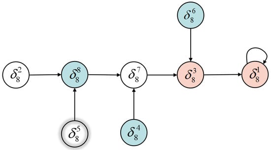
Figure 1. The state transition diagram of Example 3.

6. Conclusions

In this paper, set stability and set stabilization avoiding undesirable set of BNs and BCNs have been investigated, respectively. Using the STP of matrices, necessary and sufficient conditions for set reachability and set stability of BNs and BCNs with constraint states have been obtained, respectively. In addition, for BNs and BCNs, the formulas for calculating the transition period from each state of initial set to a given destination set have been given, respectively. Based on the transition period, a design method of the time optimal stabilizer is proposed.

By means of matrix $L_{\Omega }$, the test method of reachability from one state to the others was given. Moreover, we constructed the set stability vector H (set stabilization vector $H_C$) based on constrained matrix $L_{\Omega }$, which can give the criteria of set stability (set stabilization) under the state constraint in vector form. It is noted that all the calculations involved are matrix operations, which are easy to validate by mathematical software. In general, all the results in this paper can be extended to mixed-valued logical (control) networks. The method proposed in this paper is helpful to the study of partial stability and partial stabilization under state constraints.

However, computational complexity is the main obstacle to study large-scale logical (control) networks using STP. In this paper, the set stability under state constraints was studied theoretically. We will consider the problem of reducing computational complexity in the future.

References

- Kauffman, S.A. Metabolic stability and epigenesis in randomly constructed genetic nets. J. Theor. Biol. 1969, 22, 437–467. [Google Scholar] [CrossRef]
- Akutsu, T.; Hayashida, M.; Ching, W.K.; Ng, M.K. Control of Boolean networks: Hardness results and algorithms for tree structured networks. J. Theor. Biol. 2007, 244, 670–679. [Google Scholar] [CrossRef] [PubMed]
- Albert, R.; Barabási, A.L. Dynamics of complex systems: Scaling laws for the period of Boolean networks. Phys. Rev. Lett. 2000, 84, 5660. [Google Scholar] [CrossRef] [PubMed] [Green Version]
- Fauré, A.; Naldi, A.; Chaouiya, C.; Thieffry, D. Dynamical analysis of a generic Boolean model for the mammalian cell cycle. Bioinformatics 2006, 22, e124–e131. [Google Scholar] [CrossRef] [Green Version]
- Shmulevich, I. On the Lyapunov Exponent of Monotone Boolean Networks. Mathematics 2020, 8, 1035. [Google Scholar] [CrossRef]
- Rämö, P.; Kesseli, J.; Yli-Harja, O. Stability of functions in Boolean models of gene regulatory networks. Chaos 2005, 15, 034101. [Google Scholar] [CrossRef] [PubMed]
- Walker, C.C. Stability of equilibrial states and limit cycles in sparsely connected, structurally complex Boolean nets. Complex Syst. 1987, 1, 1063–1086. [Google Scholar]
- Watta, P.B.; Wang, K.; Shringarpure, R. Dynamical Boolean systems: Stability analysis and applications. In Proceedings of the SPIE’s 1995 Symposium on OE/Aerospace Sensing and Dual Use Photonics, SPIE 2492, Orlando, FL, USA, 17 April 1995; pp. 512–523. [Google Scholar]
- Bilke, S.; Sjunnesson, F. Stability of the Kauffman model. Phys. Rev. E 2001, 65, 016129. [Google Scholar] [CrossRef] [Green Version]
- Cheng, D.; Qi, H.; Zhao, Y. An Introduction to Semi-Tensor Product of Matrices and Its Applications; World Scientific: Singapore, 2012. [Google Scholar]
- Cheng, D.; Qi, H. Analysis and Control of Boolean Networks: A Semi-Tensor Product Approach; Springer: London, UK, 2011. [Google Scholar]
- Cheng, D.; Qi, H. A linear represeatation of dynamics of Boolean networks. IEEE Trans. Autom. Control 2010, 55, 2251–2258. [Google Scholar] [CrossRef]
- Zhu, Q.; Gao, Z.; Liu, Y.; Gui, W. Categorization problem on controllability of boolean control networks. IEEE Trans. Autom. Control 2020, 66, 2297–2303. [Google Scholar] [CrossRef]
- Jiang, B.; Liu, Y.; Kou, K.; Wang, Z. Controllability and observability of linear quaternion-valued systems. Acta Math. Sin. Engl. Ser. 2021, 36, 1299–1314. [Google Scholar] [CrossRef]
- Yu, Y.; Meng, M.; Feng, J.E. Observability of Boolean networks via matrix equations. Automatica 2020, 111, 108621. [Google Scholar] [CrossRef]
- Yang, Y.; Liu, Y.; Lou, J.; Wang, Z. Observability of switched Boolean control networks using algebraic forms. Discret. Contin. Dyn. Syst.-S 2021, 14, 1519–1533. [Google Scholar] [CrossRef]
- Wu, Y.; Guo, Y.; Toyoda, M. Policy iteration approach to the infinite horizon average optimal control of probabilistic Boolean networks. IEEE Trans. Neural Netw. Learn. Syst. 2021, 32, 2910–2924. [Google Scholar] [CrossRef]
- Li, H.; Wang, S.; Li, X.; Zhao, G. Perturbation analysis for controllability of logical control networks. SIAM J. Control Optim. 2020, 58, 3632–3657. [Google Scholar] [CrossRef]
- Wang, S.; Li, H. Graph-based function perturbation analysis for observability of multi-valued logical networks. IEEE Trans. Neural Netw. Learning Syst. 2020. [Google Scholar] [CrossRef]
- Wang, S.; Li, H. Resolution of fuzzy relational inequalities with Boolean semi-tensor product composition. Mathematics 2021, 9, 937. [Google Scholar] [CrossRef]
- Lu, J.; Li, B.; Zhong, J. A novel synthesis method for reliable feedback shift registers via Boolean networks. Sci. China Inf. Sci. 2021, 64, 152207. [Google Scholar] [CrossRef]
- Guo, Y.; Wu, Y.; Gui, W. Stability of discrete-time systems under restricted switching via logic dynamical generator and STP-based mergence of hybrid states. IEEE Trans. Autom. Control 2021. [Google Scholar] [CrossRef]
- Wu, J.; Zhong, J.; Liu, Y.; Gui, W. State Estimation of Networked Finite State Machine with Communication Delays and Losses. IEEE Trans. Circuits Syst. II Express Briefs 2021. [Google Scholar] [CrossRef]
- Liu, Z.; Zhong, J.; Liu, Y.; Gui, W. Weak Stabilization of Boolean Networks Under State-Flipped Control. IEEE Trans. Neural Netw. Learn. Syst. 2021. [Google Scholar] [CrossRef]
- Fu, S.; Zhao, J.; Wang, J. Input-output decoupling control design for switched Boolean control networks. J. Frankl. Inst. 2018, 355, 8576–8596. [Google Scholar] [CrossRef]
- Li, H.; Yang, X.; Wang, S. Robustness for stability and stabilization of Boolean networks with stochastic function perturbations. IEEE Trans. Autom. Control 2021, 66, 1231–1237. [Google Scholar] [CrossRef]
- Chen, H.; Liang, J.; Lu, J. Partial synchronization of interconnected Boolean networks. IEEE Trans. Cybern. 2017, 47, 258–266. [Google Scholar] [CrossRef] [PubMed]
- Li, Y.; Li, H.; Wang, S. Finite-time consensus of finite field networks with stochastic time delays. IEEE Trans. Circuits Syst. II Express Briefs 2020, 67, 3128–3132. [Google Scholar] [CrossRef]
- Guo, Y.; Wang, P.; Gui, W.; Yang, C. Set stability and set stabilization of Boolean control networks besed on invariant subsets. Automatica 2015, 61, 106–112. [Google Scholar] [CrossRef]
- Li, F.; Li, H.; Xie, L. On stabilization and set stabilization of multivalued logical systems. Automatica 2017, 80, 41–47. [Google Scholar] [CrossRef]
- Sui, H. Gene expression profiling, genetic networks, and cellular states: An integrating concept for tumorigenesis and drug discovery. J. Mol. Med. 1999, 77, 469–480. [Google Scholar] [CrossRef]
- Xiao, Y.; Dougherty, E. The impact of function perturbations in Boolean networks. Bioinformatics 2007, 23, 1265–1273. [Google Scholar] [CrossRef] [Green Version]
- Li, Z.; Song, J. Controllability of Boolean control networks avoiding states set. Sci. China Inf. Sci. 2014, 57, 1–13. [Google Scholar] [CrossRef]
- Guo, Y.; Ding, Y. Observability of Boolean control networks with input constraints. In Proceedings of the 2017 13th IEEE International Conference on Control & Automation (ICCA), Ohrid, Macedonia, 3–6 July 2017; pp. 719–722. [Google Scholar]
- Li, Y.; Li, H.; Li, Y. Constrained set controllability of logical control networks with state constraints and its applications. Appl. Math. Comput. 2021, 405, 126259. [Google Scholar] [CrossRef]
- Montalva-Medel, M.; Ledger, T.; Ruz, G.A.; Goles, E. Lac Operon Boolean Models: Dynamical Robustness and Alternative Improvements. Mathematics 2021, 9, 600. [Google Scholar] [CrossRef]
Publisher’s Note: MDPI stays neutral with regard to jurisdictional claims in published maps and institutional affiliations. |
© 2021 by the authors. Licensee MDPI, Basel, Switzerland. This article is an open access article distributed under the terms and conditions of the Creative Commons Attribution (CC BY) license (https://creativecommons.org/licenses/by/4.0/).