Sound Localization through Multi-Scattering and Gradient-Based Optimization

Abstract

A gradient-based optimization (GBO) method is presented for acoustic lens design and sound localization. GBO uses a semi-analytical optimization combined with the principle of acoustic reciprocity. The idea differs from earlier inverse designs that use topology optimization tools and generic algorithms. We first derive a formula for the gradients of the pressure at the focal point with respect to positions of a set of cylindrical scatterers. The analytic form of the gradients enhances modeling capability when combined with optimization algorithms and parallel computing. The GBO algorithm maximizes the sound amplification at the focal point and enhances the sound localization by evaluating pressure derivatives with respect to the cylinder positions and then perturbatively optimizing the position of each cylinder in the lens while incorporating multiple scattering between the cylindrical scatterers. The results of the GBO of the uni- and multi-directional broadband acoustic lens designs are presented including several performance measures for the frequency dependence and the incidence angle. A multi-directional broadband acoustic lens is designed to localize the sound and to focus acoustic incident waves received from multiple directions onto a predetermined localization region or focal point. The method is illustrated for configurations of sound hard and sound soft cylinders as well as clusters of elastic thin shells in water.

1. Introduction

Metamaterials are engineered materials that can control and guide the energy flow with capabilities exceeding those possible in conventional materials, enabling the control of acoustic, electromagnetic, and mechanical waves. Despite the exciting results obtained by the physics-inspired metamaterial designs, the forward design methodology relies on tuning parameters by trial and error where the low efficiency and limited exploration of the design variations lean to miss out the optimal solution. Using the inverse design approaches, one can start from the opposite end and optimize certain objective functions describing the desired functionality. The progress in inverse design has led to the discovery of metastructures with exceptional performances. Among various methods, large-scale gradient-based optimization (GBO) [1,2] has been a popular approach to design structures containing a vast number of degrees of freedom. The adjoint method [3] was employed in optimization of elastic and acoustic metamaterials [4,5], and of nanophotonic devices [6,7]. Topology optimization was utilized to design metasurfaces [8,9,10] and acoustic cloak composed of bimode on a honeycomb lattice [11], to improve the vibro-acoustic response of 3D sandwich panels [12] and predict structural parameters of 3D lattice structures [13,14], bi-mode materials [15], and mechanical metamaterials [16]. Popa and Cummer [17] proposed an optimization approach which produced simplified, broadband omnidirectional designs of transformation optics devices. A level set-based topology optimization using the FEM was employed in inverse design of optical hyperlens by Otomori et al. [18].

Placement optimization is commonly used to arrange scatterers or sources in acoustic/elastodynamic/thermal fields using genetic algorithms [19]. Håkansson et al. used multiple scattering theory and genetic algorithms in the inverse design of photonic crystals [20] and flat acoustic lenses [21,22]. Lu et al. [23] proposed an acoustic cloak design based on Bézier scatterers using genetic algorithms (GA) and simulated annealing. These GA used for optimization are gradient-free. The number of iterations needed before the solution converges tend to be large as the complexity of the model grows and as the number of design parameters increases. Stochastic algorithms do not require the evaluation of the objective function, but, if available, the analytical form of the gradients can enhance the quality and precision of the global optimal solution [24,25]. The function evaluations required in non-gradient optimization algorithms are orders of magnitude more than that is required for GBO methods [26]. In comparison to gradient-free based algorithms, GBO utilizes additional derivative information with respect to the design parameters that can result in a reduced number of iterations. The accuracy of solutions obtained with GBO algorithms [27] exceeds those obtained with stochastic algorithms. Erikson [19] performed a thermal design optimization with design parameters based on geometric properties such as length, width, angle, or position of the heat sources by solving PDE constrained optimization problem using fmincon solver and sequential quadratic programming (SQP) algorithms. In this model, Erikson [19] showed that the final optimal solution depended on the boundary conditions and the profile of the ingoing velocity field applied, and considered a loop over several random initial positions to find the best optimal solution which varied as the convective field and the ambient temperature changed. The gradient-based approach was developed by Amirkulova and Norris to design an acoustic cloak [28,29,30] and lens [31,32]. Andersen et al. [27] designed a multi-directional acoustic cloak by means of the boundary element method and shape optimization using the gradient-based SQP algorithm with the fmincon solver [33]. Chen et al. [34] discussed level set and eigenfunction optimization methods to represent the topography of a dielectric media and discussed gradient-based methods to solve different material design problems. McCormick and Shepherd [35] provided a comparison of performance gradient-based, fmincon [33], and evolutionary, Borg, algorithms to minimize the vibration response within a certain region of the beam at discrete frequencies, with constraints on total mass and static compliance. However, in their simulations [35] with fmincon, the analytical formulas for the gradients were not provided and the fmincon solver computed the gradients numerically using finite differences which requires additional runtime to compute the gradients. As these numerical gradients are not exact, fmincon produces poorer results as opposed to the case when gradients are evaluated analytically and supplied to fmincon.

In this paper, we explore the directionality and frequency band efficiency associated with focusing and localization effects based on discrete scatterers and show some ways to overcome limitations. We obtain a semi-analytical formula for the gradient of the pressure at the focal point with respect to positions of a set of cylindrical scatterers using two approaches namely forward and reciprocal formulations. We combine these formulae with GBO algorithms and apply them to design a uni- and multi-incidence-directional broadband lens by means of multiple scattering theory and applying the principle of reciprocity. A broad review of the literature on single and multiple scattering and of the concepts of multiple scattering is given in [36]; a survey of more recent findings on multiple scattering from obstacles in acoustic and elastic media is provided in [37]. In our model, an acoustic lens consists of a meta-cluster of rigid cylinders, cylindrical voids, or a set of elastic shells submerged in water. We design metastructures made of conventional simple isotropic materials that are available in nature and obtain useful and interesting effects. The idea differs from earlier inverse designs that use topology optimization tools and generic algorithms. The GBO algorithm maximizes the sound amplification at the focal point by evaluating pressure derivative with respect to the cylinder positions and then perturbatively optimizing the position of each cylinder in the lens while taking into account acoustic the multiple scattering between the cylinders. Computations are performed on MATLAB using advanced parallel optimization algorithms and a MultiStart optimization solver, and supplying the gradient of absolute pressure amplitude at the focal point.

The paper is organized as follows. Section 2 starts with a definition of multiple scattering problem, the position-dependent absolute acoustic pressure at the focal point, and the principle of acoustic reciprocity for this problem. Gradients of the absolute acoustic pressure at the focal point with respect to cylinder positions are then obtained by means of multiple scattering theory for forward and reciprocal formulations. Some properties of the gradient vectors are illustrated through numerical examples in Section 2.6. Application of the closed form for the gradient of absolute acoustic pressure at the focal point to acoustic lens designs are given in Section 3. Single and broadband as well as uni- and multi-directional focusing effects are illustrated using multiple reconfigurable cylinders as the lensing and localization mechanisms.

2. Problem Definition

We consider multiple acoustic scattering in two dimensions. Starting from the linear wave equation for an acoustic medium with sound speed c, and assuming time harmonic dependence $e^{-i\omega t}$ of frequency $\omega$ results in the the Helmholtz equation for the acoustic pressure $p\left(\mathbf{x}\right)$,

$${\nabla }^{2}p\left(\mathbf{x}\right)+k^{2}p\left(\mathbf{x}\right)=0,$$

(1)

where $k=\omega /c$ is the wavenumber, c is the acoustic speed, and $\mathbf{x}$ is the position vector of point P with respect to origin O (see Figure 1). The factor $e^{-i\omega t}$ is omitted in the following. The total field p is the sum of incident $p_{inc}$ and scattered $p_{sc}$ pressure fields:

$$p\left(\mathbf{x}\right)=p_{inc}\left(\mathbf{x}\right)+p_{sc}\left(\mathbf{x}\right).$$

(2)

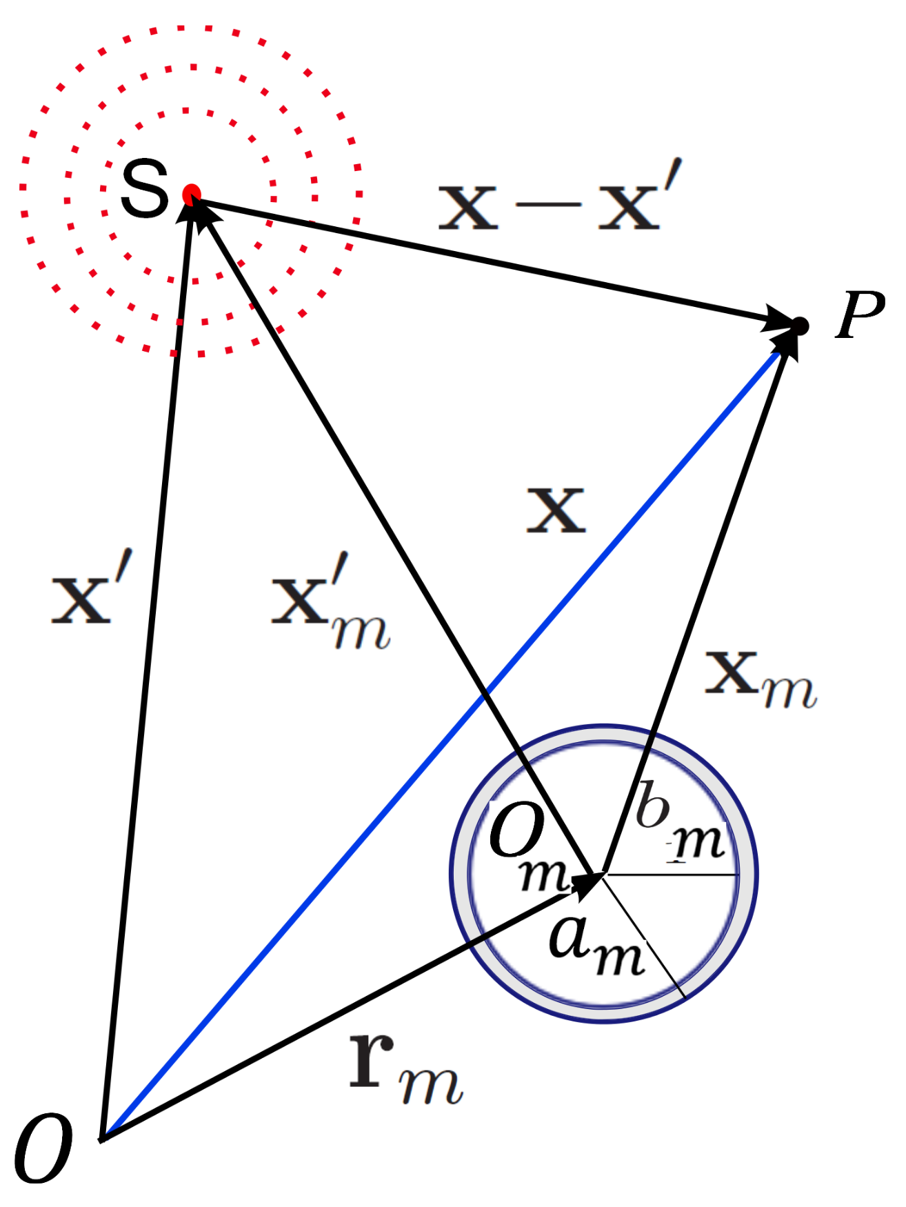
Figure 1. An arbitrary planar configuration of M cylinders ${\mathtt{S}}_m$ with outer radius $a_m$ and inner radius $b_m$, and position vector ${\mathbf{r}}_m$, $m=\overline{1,M}$. The incident field in this case is a plane wave with wavevector $\mathbf{k}$ in the direction of angle $\psi$.

The incident field is the plane wave of unit amplitude in direction $\psi$

$$p_{inc}\left(\mathbf{x}\right)=e^{ik{\mathbf{e}}_{\psi }·\mathbf{x}}.$$

(3)

Our objective is to maximize the acoustic pressure at the predefined focal point ${\mathbf{x}}_f$ by rearranging the positions of M scatterers denoted by the set of vectors $\left\{{\mathbf{r}}_m\right\}$ as shown in Figure 1. For simplicity, we take these to be circularly cylindrical scatterers, which may be either rigid cylinders or thin elastic shells illustrated in Figure 1. We define $p_f$ or equivalently $p_f\left(\left\{{\mathbf{r}}_m\right\}\right)$ to be the total acoustic pressure at the focal point for a given set $\left\{{\mathbf{r}}_m\right\}$, i.e.,

$$p_f\left(\left\{{\mathbf{r}}_m\right\}\right)=p\left({\mathbf{x}}_f\right).$$

(4)

As a measure of the scattering we use the sound amplification, $S{A}_f$, at the focal point defined as

$$S{A}_f\left(dB\right)=20l{g}_{10}\left(\frac{|p_f\left(\left\{{\mathbf{r}}_m\right\}\right)|}{|p_{inc}\left({\mathbf{x}}_f\right)|}\right),$$

(5)

where the absolute value is $\left|p\right|={\left(p{p}^{*}\right)}^{1/2}$, and ∗ denotes the complex conjugate. The objective is to maximize $S{A}_f$ by rearranging the cylinders to find an optimal set $\left\{{\mathbf{r}}_m\right\}$. The critical quantity that we use in the process is the gradient of the acoustic pressure at the focal point, defined next.

2.1. Position-Dependent Acoustic Pressure Field at the Focal Point

We employ multiple scattering theory to solve for the pressure at the focal point. Each scatterer, denoted by index m, radiates as a localized source, with multipole strengths $B_n^{\left(m\right)}$ where n denotes the dependence on angle, $e^{in\theta }$. Thus, according to (A8), the scattered field in the neighborhood of cylinder ${\mathtt{S}}_m$ is given by

$$p_{sc}\left(\mathbf{x}\right)=\sum _{m=1}^M\sum _{n=-\infty }^{\infty }{B}_n^{\left(m\right)}{V}_n^{+}\left({\mathbf{x}}_m\right),$$

(6)

where $B_n^{\left(m\right)}$ are the unknown coefficients, and ${\mathbf{x}}_m$ is the position vector of point P with respect to the cylinder center at $O_m$:

$${\mathbf{x}}_m=\mathbf{x}-{\mathbf{r}}_m$$

(7)

The functions $V_n^{\pm }\left(\mathbf{x}\right)$, defined in Equation (A9), are

$$V_n^{\pm }\left(\mathbf{x}\right)=H_n^{\left(1\right)}\left(k\right|\mathbf{x}\left|\right)e^{\pm inarg\mathbf{x}}$$

(8)

where $H_n^{\left(1\right)}$ is the Hankel function of the first kind of order n, $arg\mathbf{x}$ denotes the argument of vector $\mathbf{x}$, i.e., the angle that the vector $\mathbf{x}$ makes with the positive x-axis, and it is measured as $arg\mathbf{x}\in [0,2\pi )$ and $arg\left(-\mathbf{x}\right)=(arg(\mathbf{x})\pm \pi )mod2\pi$ [38]. Introducing Equations (3) and (6) into Equation (2), and evaluating it at the focal point $P_f$, defines the total pressure at the fixed focal point:

$$p_f=e^{ik{\mathbf{e}}_{\psi }·{\mathbf{x}}_f}+\sum _{m=1}^M\sum _{n=-\infty }^{\infty }{B}_n^{\left(m\right)}{V}_n^{+}({\mathbf{x}}_f-{\mathbf{r}}_m).$$

(9)

In order to apply the solution Equation (9) in practice, the infinite sum must be truncate. Let N be the truncation value of the infinite sum in Equation (9) chosen so that the sum converges. In practice, the value of N depends upon frequency and typically taking the truncation number $N\approx 2.5$ ka is adequate [29]. Let us introduce the vectors $\mathbf{b},\mathbf{v}\in {𝒞}^{M\times (2N+1)}$. The components of the scattering coefficient vector $\mathbf{b}=\left\{B_n^{\left(j\right)}\right\}$, $j\in (1,M)$, $n\in (-N,N)$, are $B_n^{\left(j\right)}=\left\{B_n\left({\mathbf{r}}_j\right)\right\}$ found from Equations (A21) and (A22), and written in column vector form:

$$\mathbf{b}=\left(\begin{array}{c}{\mathbf{b}}^{\left(1\right)}\\ {\mathbf{b}}^{\left(2\right)}\\ ⋮\\ {\mathbf{b}}^{\left(M\right)}\end{array}\right),{\mathbf{b}}^{\left(j\right)}=\left(\begin{array}{c}{B}_{-N}^{\left(j\right)}\\ B_{-N+1}^{\left(j\right)}\\ ⋮\\ B_N^{\left(j\right)}\end{array}\right).$$

(10)

The elements of the dual vector $\mathbf{v}=\left\{V_n^{\left(j\right)}\right\}=\left\{V_n\left({\mathbf{r}}_j\right)\right\}$ are of the form

$$\begin{array}{c}\hfill V_n^{\left(m\right)}=V_n^{+}\left({\mathbf{r}}_{fm}\right),\end{array}$$

(11)

where

$${\mathbf{r}}_{fm}={\mathbf{x}}_f-{\mathbf{r}}_m,$$

(12)

is the position of focal point with respect to local coordinate at $O_m$ and ${\mathbf{r}}_m$ is the position of scatterer with respect to origin at O. Then, the total pressure field at the focal point can be written in vector form as

$$p_f=e^{ik{\mathbf{e}}_{\psi }·{\mathbf{x}}_f}+{\mathbf{v}}^T\mathbf{b}.$$

(13)

The Scattering Strengths

The scattering problem is solved once we have the scattering strengths, represented by the column vector $\mathbf{b}$ which solves the linear system of equations

$$\mathbb{X}\mathbf{b}=\mathbf{a},$$

(14)

where

$$\mathbf{a}=\left(\begin{array}{c}{\mathbf{a}}^{\left(1\right)}\\ {\mathbf{a}}^{\left(2\right)}\\ ⋮\\ {\mathbf{a}}^{\left(M\right)}\end{array}\right),{\mathbf{a}}^{\left(j\right)}=\left(\begin{array}{c}{A}_{-N}^{\left(j\right)}\\ A_{-N+1}^{\left(j\right)}\\ ⋮\\ A_N^{\left(j\right)}\end{array}\right).$$

(15)

The elements of the column vector $\mathbf{a}\in {\mathcal{C}}^{M\times (2N+1)}$ are defined such that $\mathbf{a}=\left\{A_n^{\left(j\right)}\right\}=\left\{A_n\left({\mathbf{r}}_j\right)\right\}$, where

$$A_n^{\left(m\right)}=A_n\left({\mathbf{r}}_m\right)=\left\{\begin{array}{c}{i}^n{e}^{ik{x}_m},\mathrm{for}\mathrm{a}\mathrm{normal}\mathrm{incidence}\psi =0,\mathrm{where}{x}_m={\mathbf{e}}_1·{\mathbf{r}}_m,\hfill \\ i^n{e}^{ik(x_{m}cos\psi +y_{m}sin\psi )}{e}^{-in\psi },\mathrm{for}\mathrm{a}\mathrm{general}\mathrm{incident}\mathrm{angle}\psi ,\hfill \end{array}\right.$$

(16)

for $n\in [-N,N]\mathrm{and}N\in \mathbb{Z}$. Here, the matrix $\mathbb{X}$ is the interaction matrix that defines the coupling between each scatterer of the configuration (see Appendix A.1 for details)

$$\mathbb{X}=\left[\begin{array}{ccccc}{{\mathbf{T}}^{\left(1\right)}}^{-1}& -{\mathbf{P}}^{1,2}& -{\mathbf{P}}^{1,3}& \cdots & -{\mathbf{P}}^{1,M}\\ -{\mathbf{P}}^{2,1}& {{\mathbf{T}}^{\left(2\right)}}^{-1}& -{\mathbf{P}}^{2,3}& \cdots & -{\mathbf{P}}^{2,M}\\ ⋮& ⋮& ⋮& \ddots & ⋮\\ -{\mathbf{P}}^{M,1}& -{\mathbf{P}}^{M,2}& -{\mathbf{P}}^{M,3}& \cdots & {{\mathbf{T}}^{\left(M\right)}}^{-1}\end{array}\right].$$

(17)

The matrix ${\mathbf{T}}^{\left(j\right)}$ is the transition or T-matrix for scatterer j, and ${\mathbf{P}}^{j,m}=\left[{\mathbf{P}}_{ql}^{j,m}\right]$ is a Toeplitz matrix that depends on the position vector ${\mathbf{r}}_{jm}$ depicted in Figure 1. The matrix ${\mathbf{P}}^{j,m}$ takes into account the interaction between the scatterers, whereas the transition matrix ${\mathbf{T}}^{\left(j\right)}$ depends on the shape and the physical properties of the material of cylinder, as well as the boundary conditions on the interfaces. The T-matrix is diagonal for scatterers with rotational symmetry. In general, for an obstacle with no rotational symmetry, e.g., an elastic thin cylindrical shell with internal spring-mass attachments [39], the T-matrix is nondiagonal. The off-diagonal terms couple different azimuthal orders of the incident and scattered field. At low frequency, the T-matrix may be truncated as a 3 × 3 matrix, in which case off-diagonal elements can be interpreted in terms of Willis coupling [40]. In this work, we consider 2-dimensional configurations of circularly cylindrical scatterers, for which the T-matrices become diagonal, see in [37] for specific details. In particular, ${\mathbf{P}}^{j,m}=\left[P_{ql}^{j,m}\right]$ for $j,m\in (1,M),j\ne m,l,q\in (-N,N)$,

$$P_{ql}^{j,m}=P_{ql}\left({\mathbf{r}}_{jm}\right)=H_{l-q}^{\left(1\right)}\left(k{r}_{jm}\right)e^{i(l-q)arg{\mathbf{r}}_{jm}}$$

(18)

where ${\mathbf{r}}_{jm}={\mathbf{r}}_j-{\mathbf{r}}_m$, $arg\mathbf{x}\in [0,2\pi )$. Alternatively, the acoustic pressure field at fixed focal point can be determined in a simpler form using the principle of acoustic reciprocity which is described next.

2.2. Acoustic Reciprocity

Here, we will illustrate the use of acoustic reciprocity [41] to define the pressure at the focal point $P_f$ due to a source located in a far-field. The key result is that the acoustic pressure at position ${\mathbf{x}}_i$ due to a monopole source at position ${\mathbf{x}}_f$ is identical to the pressure at ${\mathbf{x}}_f$ resulting from a monopole of the same strength located at ${\mathbf{x}}_i$. This reciprocity enables us to relate the response for an incident plane wave in terms of the far-field Green’s function.

We apply the reciprocity result to this problem by first considering two points ${\mathbf{x}}_f$ and ${\mathbf{x}}_i$ illustrated in Figure 2. In the forward problem, FP, the source is at ${\mathbf{x}}_i$ and the pressure is computed at ${\mathbf{x}}_f$:

$$p_{f;i}=p({\mathbf{x}}_f;{\mathbf{x}}_i)$$

(19)

where $p(\mathbf{x};\mathbf{y})$ is the total acoustic pressure at $\mathbf{x}$ for a point source at $\mathbf{y}$, which corresponds to a non-zero delta term on the right hand side of Equation (1). In the reciprocal problem, RP, the source is at ${\mathbf{x}}_f$ and the pressure is computed at ${\mathbf{x}}_i$:

$$p_{i;f}=p({\mathbf{x}}_i;{\mathbf{x}}_f).$$

(20)

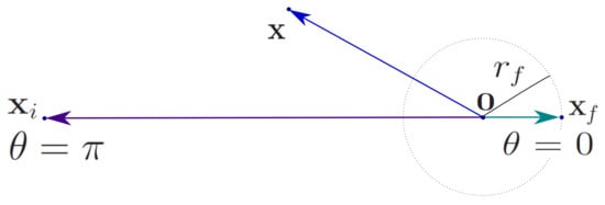
Figure 2. Near-field and far-field.

By reciprocity we have

$$p_{i;f}=p_{f;i}.$$

(21)

We take ${\mathbf{x}}_i$ in the far-field (see Figure 2), i.e., such that $k|{\mathbf{x}}_i|\gg 1$, and choose the monopole amplitude such that the source at ${\mathbf{x}}_i$ yields a plane wave of unit amplitude in the vicinity of $\mathbf{x}=\mathbf{0}$, which is the incident wave for FP. Therefore, the source, or incident wave, for RP is

$$p_{inc}\left(\mathbf{x}\right)=D_0{H}_0^{\left(1\right)}\left(k\right|\mathbf{x}-{\mathbf{x}}_f\left|\right),\mathrm{where}{D}_0={\left(i\frac{\pi }{2}k\left|{\mathbf{x}}_i\right|\right)}^{1/2}{e}^{-ik|{\mathbf{x}}_i|}.$$

(22)

Note that in this case in the local coordinates of multipole centered at $O_m$:

$$\mathbf{x}-{\mathbf{x}}_f={\mathbf{x}}_m-{\mathbf{r}}_{fm},$$

(23)

where ${\mathbf{x}}_m$ and ${\mathbf{r}}_{fm}$ are correspondingly the position vectors of an arbitrary point P and a source S with respect to $O_m$. Thus, using the Graf’s addition theorem (A10) in the neighborhood of cylinder ${\mathtt{S}}_m$ (see Figure 1), we have

$$p_{inc}=D_0{H}_0^{\left(1\right)}\left(k\right|\mathbf{x}-{\mathbf{x}}_f\left|\right)=D_0\sum _{n=-\infty }^{\infty }\left\{\begin{array}{cc}{V}_n^{+}\left({\mathbf{x}}_m\right)U_n^{-}\left({\mathbf{r}}_{fm}\right),\hfill & |{\mathbf{x}}_m|>|{\mathbf{r}}_{fm}|,\hfill \\ U_n^{+}\left({\mathbf{x}}_m\right)V_n^{-}\left({\mathbf{r}}_{fm}\right),\hfill & |{\mathbf{x}}_m|<|{\mathbf{r}}_{fm}|,\hfill \end{array}\right.$$

(24)

for $m=\overline{1,M},n\in \mathbb{Z}$, where $U_n^{\pm }$ and $V_n^{\pm }$ are defined by (A11). Ultimately we consider $|{\mathbf{x}}_m|<|{\mathbf{r}}_{fm}|$ to compute pressure and apply boundary conditions at the interface $|{\mathbf{x}}_m|=a_m$. Thus, for $|{\mathbf{x}}_m|<|{\mathbf{r}}_{fm}|$, near cylinder $S_m$ we have

$$p_{inc}=D_0\sum _{n=-\infty }^{\infty }{U}_n^{+}\left({\mathbf{x}}_m\right)V_n^{-}\left({\mathbf{r}}_{fm}\right)\Rightarrow p_{inc}^{\left(m\right)}=\sum _{n=-\infty }^{\infty }{D}_n^{\left(m\right)}{U}_n^{+}\left({\mathbf{x}}_m\right),$$

(25)

where

$$D_n^{\left(m\right)}=D_n\left({\mathbf{r}}_m\right)=D_0{V}_n^{-}\left({\mathbf{r}}_{fm}\right)$$

(26)

We now consider the reciprocal problem by examining a monopole source located at position ${\mathbf{x}}_f$ at the focal point $P_f=(r=r_f,\theta =0)$. Then, according to Equation (A23), the far-field radiated by source at $P_f$ is

$$p^{sc}({\mathbf{x}}_i;{\mathbf{x}}_f)=p^{sc}(R_i,\theta =\pi )=f\left(\pi \right)\sqrt{\frac{k}{i2\pi |{\mathbf{x}}_i|}}{e}^{ik|{\mathbf{x}}_i|}\left[1+O\left(\frac{1}{k|{\mathbf{x}}_i|}\right)\right],$$

(27)

where the far-field amplitude function in the direction of ${\mathbf{x}}_i$ is

$$f\left(\pi \right)=\frac{2}{k}\sum _{n=-\infty }^{\infty }\sum _{m=1}^M{i}^n{e}^{ik{x}_m}{\widehat{B}}_n^{\left(m\right)}.$$

(28)

The scattering coefficients ${\widehat{B}}_n^{\left(j\right)}=\{{\widehat{B}}_n^{\left(j\right)}\}=\{{\widehat{B}}_n\left({\mathbf{r}}_j\right)\}$, $j\in (1,M)$, $n\in (-N,N)$ are components of the dual vector $\widehat{\mathbf{b}}$ that satisfies the multiple scattering condition

$$\mathbb{X}\widehat{\mathbf{b}}=\mathbf{d},$$

(29)

where $\mathbb{X}$ is the interaction matrix defined by Equation (17). The elements of the dual vector $\mathbf{d}=\{D_n^{\left(j\right)}\}=\left\{D_n\left({\mathbf{x}}_{mf}\right)\right\}$ are defined by Equation (26). The vectors $\widehat{\mathbf{b}},\mathbf{d}\in {\mathcal{C}}^{M\times (2N+1)}$ are defined such that

$$\mathbf{d}=\left(\begin{array}{c}{\mathbf{d}}^{\left(1\right)}\\ {\mathbf{d}}^{\left(2\right)}\\ ⋮\\ {\mathbf{d}}^{\left(M\right)}\end{array}\right),\widehat{\mathbf{b}}=\left(\begin{array}{c}{\widehat{\mathbf{b}}}^{\left(1\right)}\\ {\widehat{\mathbf{b}}}^{\left(2\right)}\\ ⋮\\ {\widehat{\mathbf{b}}}^{\left(M\right)}\end{array}\right),{\mathbf{d}}^{\left(j\right)}=\left(\begin{array}{c}{D}_{-N}^{\left(j\right)}\\ D_{-N+1}^{\left(j\right)}\\ ⋮\\ D_N^{\left(j\right)}\end{array}\right),{\widehat{\mathbf{b}}}^{\left(j\right)}=\left(\begin{array}{c}{\widehat{B}}_{-N}^{\left(j\right)}\\ {\widehat{B}}_{-N+1}^{\left(j\right)}\\ ⋮\\ {\widehat{B}}_N^{\left(j\right)}\end{array}\right).$$

(30)

The far-field amplitude function (28) can then be expressed as

$$f\left(\pi \right)=\frac{2}{k}{\mathbf{a}}^T\widehat{\mathbf{b}}$$

(31)

and

$$p^{sc}({\mathbf{x}}_i;{\mathbf{x}}_f)=\gamma {\mathbf{a}}^T\widehat{\mathbf{b}}$$

(32)

where $\gamma =\sqrt{\frac{2}{ik\pi |{\mathbf{x}}_i|}}{e}^{ik|{\mathbf{x}}_i|}$. By reciprocity principle, Equation (21), the resultant total pressure at the fixed focal point $P_f$ at $\theta =0$ by a plane wave incidence from $\theta =\pi$ can be written as

$$p_f=p({\mathbf{x}}_f;{\mathbf{x}}_i)=e^{ik{\mathbf{e}}_1·{\mathbf{x}}_f}+\gamma {\mathbf{a}}^T\widehat{\mathbf{b}}.$$

(33)

This is to be compared with the solution (13) obtained by solving the direct multiple scattering problem. Of course, by reciprocity both are equal.

2.3. The Gradient Vectors ${\mathbf{q}}_j$ and ${\mathbf{p}}_j$

The real valued vector ${\mathbf{q}}_j$ is defined as gradient of the absolute value of total pressure field $|p_f\left(\left\{{\mathbf{r}}_m\right\}\right)|$ with respect to positions ${\mathbf{r}}_j$. It can can be evaluated as

$$\begin{array}{c}\hfill {\mathbf{q}}_j=\frac{\partial |p_f|}{\partial {\mathbf{r}}_j}=\frac{1}{2|p_f|}\frac{\partial |p_f{|}^2}{\partial {\mathbf{r}}_j}=\frac{1}{2|p_f|}\left(\frac{\partial p_f}{\partial {\mathbf{r}}_j}{p}_f^{*}+p_f\frac{\partial p_f^{*}}{\partial {\mathbf{r}}_j}\right)=\frac{1}{2|p_f|}\left(p_f^{*}{\mathbf{p}}_j+p_f{\mathbf{p}}_j^{*}\right)\end{array}$$

(34)

where the associated complex valued gradient vectors are

$${\mathbf{p}}_j=\frac{\partial p_f}{\partial {\mathbf{r}}_j}.$$

(35)

2.4. The Pressure Gradient by Solving the Forward Problem

We now determine the explicit form of the gradient vector using the direct and reciprocal formulations, from Equations (13) and (33), respectively.

The pressure at the focal point follows from Equations (13) and (14) as

$$p_f=e^{ik{\mathbf{e}}_{\psi }·{\mathbf{x}}_f}+{\mathbf{v}}^T{\mathbb{X}}^{-1}\mathbf{a}.$$

(36)

The complex valued gradient vectors ${\mathbf{p}}_j$ of Equation (35) can be evaluated by noting that $\frac{\partial {\mathbb{X}}^{-1}}{\partial \mathbf{x}}=-{\mathbb{X}}^{-1}\frac{\partial \mathbb{X}}{\partial \mathbf{x}}{\mathbb{X}}^{-1}$:

$${\mathbf{p}}_j=\frac{\partial {\mathbf{v}}^T}{\partial {\mathbf{r}}_j}\mathbf{b}-{\mathbf{v}}^T{\mathbb{X}}^{-1}\left(\frac{\partial \mathbb{X}}{\partial {\mathbf{r}}_j}\mathbf{b}-\frac{\partial \mathbf{a}}{\partial {\mathbf{r}}_j}\right).$$

(37)

In component form, the last Equation (37) can be written as

$$\begin{array}{cc}\hfill \left[{\mathbf{p}}_j\right]=& \sum _{m=1}^M\sum _{l=-\infty }^{\infty }\{\frac{\partial V_l^{+}({\mathbf{x}}_f-{\mathbf{r}}_m)}{\partial {\mathbf{r}}_j}{B}_l^{\left(m\right)}+V_l^{+}({\mathbf{x}}_f-{\mathbf{r}}_m)\hfill \\ \hfill \times & \sum _{i=1}^M\sum _{n=-\infty }^{\infty }{\left(X^{-1}\right)}_{lmin}\left(\frac{\partial A_n\left({\mathbf{r}}_i\right)}{\partial {\mathbf{r}}_j}-\sum _{p=1}^M\sum _{q=-\infty }^{\infty }\frac{\partial X_{inpq}}{\partial {\mathbf{r}}_j}{B}_q^{\left(p\right)}\right)\},j=\overline{1,M},\hfill \end{array}$$

(38)

where

$$\sum _{i=1}^M\sum _{n=-\infty }^{\infty }{X}_{pqin}^{-1}{X}_{inml}=\sum _{i=1}^M\sum _{n=-\infty }^{\infty }{X}_{pqin}{X}_{inml}^{-1}={\delta }_{pm}{\delta }_{ql}.$$

(39)

Define the derivative function $V_n^{\pm {}^{\prime }}\left(\mathbf{x}\right)$ as

$$U_n^{\pm {}^{\prime }}\left(\mathbf{x}\right)=J_n{}^{\prime }\left(k\right|\mathbf{x}\left|\right)e^{\pm inarg\mathbf{x}},V_n^{\pm {}^{\prime }}\left(\mathbf{x}\right)=H_n^{\left(1\right)}{}^{\prime }\left(k\right|\mathbf{x}\left|\right)e^{\pm inarg\mathbf{x}}.$$

(40)

Then based on the fact that the T-matrices are independent of position, the gradient of the components of the matrix $\mathbb{X}$ are [29]

$$\frac{\partial X_{inml}}{\partial {\mathbf{r}}_j}=\left\{\begin{array}{cc}{O}_{nl},\hfill & i=m,\hfill \\ -{\delta }_{ij}\frac{\partial P_{nl}}{\partial {\mathbf{r}}_j}\left({\mathbf{r}}_{jm}\right)-{\delta }_{mj}\frac{\partial P_{nl}}{\partial {\mathbf{r}}_j}\left({\mathbf{r}}_{ij}\right),\hfill & i\ne m,\hfill \end{array}\right.$$

(41)

where $O_{nl}$ are components of the zero matrix. The gradients in Equation (41) have the form [29]

$$\begin{array}{cc}\hfill \frac{\partial P_{nl}}{\partial {\mathbf{r}}_j}\left({\mathbf{r}}_{jm}\right)& =\frac{k}{r_{jm}}{V}_{l-n}^{+{}^{\prime }}\left({\mathbf{r}}_{jm}\right){\mathbf{r}}_{jm}+\frac{i(l-n)}{r_{jm}^2}{V}_{l-n}^{+}\left({\mathbf{r}}_{jm}\right){\mathbf{e}}_3\times {\mathbf{r}}_{jm},\hfill \\ \hfill \frac{\partial P_{nl}}{\partial {\mathbf{r}}_j}\left({\mathbf{r}}_{ij}\right)& =-\frac{k}{r_{ij}}{V}_{l-n}^{+{}^{\prime }}\left({\mathbf{r}}_{ij}\right){\mathbf{r}}_{ij}-\frac{i(l-n)}{r_{ij}^2}{V}_{l-n}^{+}\left({\mathbf{r}}_{ij}\right){\mathbf{e}}_3\times {\mathbf{r}}_{ij}.\hfill \end{array}$$

(42)

The gradients of the components of $\mathbf{v}$ with respect to the positions ${\mathbf{r}}_j$ of the j-th scatterer are

$$\frac{\partial V_n^{\pm }({\mathbf{x}}_f-{\mathbf{r}}_m)}{\partial {\mathbf{r}}_j}=-\left(\frac{k}{r_{fm}}{V_n^{\pm }}^{\prime }\left({\mathbf{r}}_{fm}\right){\mathbf{r}}_{fm}\pm \frac{in}{r_{fm}^2}{V}_n^{\pm }\left({\mathbf{r}}_{fm}\right){\mathbf{e}}_3\times {\mathbf{r}}_{fm}\right){\delta }_{mj},$$

(43)

where ${\mathbf{r}}_{fm}={\mathbf{x}}_f-{\mathbf{r}}_m$, $r_{fm}=|{\mathbf{x}}_f-{\mathbf{r}}_m|$, $r_j=\left|{\mathbf{r}}_j\right|$.

The gradient of the components of $\mathbf{a}$ with respect to the position ${\mathbf{r}}_j$ of the j-th scatterer is

$$\begin{array}{c}\hfill \frac{\partial {\mathbf{a}}^{\left(i\right)}}{\partial {\mathbf{r}}_j}=\sum _{q=-\infty }^{\infty }\frac{\partial A_q^{\left(i\right)}}{\partial {\mathbf{r}}_j},\end{array}$$

(44)

where for a plane wave incidence in ${\mathbf{e}}_1$ direction:

$$\begin{array}{c}\hfill \frac{\partial A_q^{\left(i\right)}}{\partial {\mathbf{r}}_j}=ik{\mathbf{e}}_1{A}_q^{\left(j\right)}{\delta }_{ij},\end{array}$$

(45)

and, hence,

$$\frac{\partial {\mathbf{a}}^{\left(i\right)}}{\partial {\mathbf{r}}_j}=ik{\mathbf{e}}_1\otimes {\mathbf{a}}^{\left(j\right)}{\delta }_{ij}.$$

(46)

The plane wave incidence in ${\mathbf{e}}_{\psi }$ direction is given by Equation (A4):

$$\begin{array}{c}\hfill \frac{\partial A_q^{\left(i\right)}}{\partial {\mathbf{r}}_j}=ik{A}_q^{\left(j\right)}{\delta }_{ij}\left(cos\psi {\mathbf{e}}_1+sin\psi {\mathbf{e}}_2\right).\end{array}$$

(47)

2.5. The Pressure Gradient by Solving the Reciprocal Problem

We now determine the explicit form of the gradient vector by solving the reciprocal problem. The pressure gradient at the focal point follows from Equations (29) and (33) as

$$\begin{array}{cc}\hfill {\widehat{\mathbf{p}}}_j=\frac{\partial p_f}{\partial {\mathbf{r}}_j}& =\frac{\partial }{\partial {\mathbf{r}}_j}\left(e^{ik{\mathbf{e}}_1·{\mathbf{x}}_f}+c{\mathbf{a}}^T{\mathbb{X}}^{-1}\mathbf{d}\right)=c\left[\frac{\partial {\mathbf{a}}^T}{\partial {\mathbf{r}}_j}\widehat{\mathbf{b}}-{\mathbf{a}}^T{\mathbb{X}}^{-1}\left(\frac{\partial \mathbb{X}}{\partial {\mathbf{r}}_j}\widehat{\mathbf{b}}-\frac{\partial \mathbf{d}}{\partial {\mathbf{r}}_j}\right)\right]\hfill \end{array}$$

(48)

where the $\widehat{}$ indicates the use of the principle of reciprocity. Of course, ${\widehat{\mathbf{p}}}_j$ of (48) should equal ${\mathbf{p}}_j$, and their equivalence is verified numerically below.

In component form, (48) can be written as

$$\begin{array}{cc}\hfill \left[{\widehat{\mathbf{p}}}_j\right]=& c\sum _{m=1}^M\sum _{l=-\infty }^{\infty }\{\frac{\partial A_l\left({\mathbf{r}}_m\right)}{\partial {\mathbf{r}}_j}{\widehat{B}}_l^{\left(m\right)}\hfill \\ \hfill +& A_l\left({\mathbf{r}}_m\right)\sum _{i=1}^M\sum _{n=-\infty }^{\infty }{\left(X^{-1}\right)}_{lmin}\left[\frac{\partial D_n\left({\mathbf{r}}_i\right)}{\partial {\mathbf{r}}_j}-\sum _{p=1}^M\sum _{q=-\infty }^{\infty }\frac{\partial X_{inpq}}{\partial {\mathbf{r}}_j}{\widehat{B}}_q^{\left(p\right)}\right]\},j=\overline{1,M},\hfill \end{array}$$

(49)

$$\begin{array}{c}\hfill \frac{\partial D_n^{\left(m\right)}}{\partial {\mathbf{r}}_j}=\frac{\partial D_n\left({\mathbf{r}}_{fm}\right)}{\partial {\mathbf{r}}_j}=D_0\frac{\partial V_n^{-}({\mathbf{x}}_f-{\mathbf{r}}_m)}{\partial {\mathbf{r}}_j},\end{array}$$

(50)

where $\frac{\partial V_n^{-}({\mathbf{x}}_f-{\mathbf{r}}_m)}{\partial {\mathbf{r}}_j}$ is defined by Equation (43), and $\widehat{\mathbf{b}}=\left\{{\widehat{B}}_l^{\left(m\right)}\right\}$ satisfies Equation (29). Other gradient components and variables are defined the same as in Section 2.4.

2.6. Numerical Examples

Before considering a sound localization problem, numerical examples will be presented for the gradient vector ${\mathbf{q}}_j$ which has some interesting characteristics. Computations are performed on MATLAB for configurations of uniform rigid cylinders of radius a. We consider two problem formulations: forward, FR, and reciprocal, RP, and make comparison of simulation times for both formulations. The reciprocal formulation of inverse design of acoustic lens takes lesser time to compute the absolute pressure and it gradients at the focal point.

2.6.1. Illustration of Principle of Reciprocity

In order to illustrate the application of reciprocity in acoustic lens design, we present numerical examples using two configurations. Figure 3a (top) shows the first configuration of a vertical setup of three cylinders of radius a and of distance $2.2a$ between each two adjacent cylinders. Figure 3 illustrates the variation of absolute pressure $p_f$ and phase angle ${\theta }_f$ at a focal point, and the gradient vector components $q_{xj}$${\widehat{q}}_{xj}$, $q_{yj}$ and ${\widehat{q}}_{yj}$ as functions of normalized wavenumber $ka$ for FR and RP formulations. The absolute pressure at a focal point that is at the point $\left(10a,0\right)$ was computed at values of normalized wavenumber $ka\in \left(0,15\right]$ using both the FP and RP methods and they coincide perfectly as shown in Figure 3a. Figure 3b presents ${\theta }_f$, the phase angle of the total pressure at the focal point versus the non-dimensional wavenumber $ka$. The gradients in the x direction are shown in Figure 3c and were computed using the FP method. The corresponding gradients that were computed using the RP method are exactly the same and they are not shown just for the clarity of the figure. The gradients in the y direction are shown in Figure 3d. They were computed using both the FR and the RP methods and they perfectly overlap. Due to the symmetry of the given configuration with respect to the x-axis, the gradients of cylinders 1 and 3 in the x direction coincide while in the y direction they have an opposite sign. Figure 4 shows the non-symmetric configuration of two rigid cylinders each of radius a, where the first is centered at the origin and the second is centered at the point $(1.5a,3a)$. The figure illustrates the dependency of absolute pressure $p_f$ and phase angle ${\theta }_f$ at a focal point $\left(10a,0\right)$ and the gradient vector components $q_{xj}$${\widehat{q}}_{xj}$, $q_{yj}$ and ${\widehat{q}}_{yj}$ as functions of normalized wavenumber $ka$ for FR and RP formulations for a non-symmetric set of two rigid cylinders. This is given to emphasize that both FP and RP methods give the same results for the non-symmetric configurations. The results of computing the absolute pressure $p_f$, the phase angle ${\theta }_f$, and the absolute pressure gradients in the x and y directions are the same for both the FR and the RP methods. The same symmetric and non-symmetric configurations were used to illustrate the non-linearity of the problem in hand. The absolute pressure was computed for the values of non-dimensional wavenumber $ka\in \left(0,15\right]$ and for the incident angle $\psi \in \left[-\pi /4,\pi /4\right]$. Figure 5c,f show the absolute pressure versus both the non-dimensional wavenumber and the incident angle. The 3D mesh plots illustrate the existence of a lot of local maxima and minima, so a small deviation in the starting optimization point and/or the incident angle and the non-dimensional wavenumber will lead to a different optimized configuration. Figure 5a,d shows the absolute pressure versus the non-dimensional wavenumber and they can be seen as the cross sectional views of the 3D plots at normal incidence: $\psi =0$. Figure 5b,e shows the absolute pressure versus the incident angle and can be seen as the cross-sectional views at $ka=7.5$.

Figure 3. Absolute pressure $p_f$ and phase angle ${\theta }_f$ at a focal point, and the gradient vector components $q_{xj}$, $q_{yj}$ and ${\widehat{q}}_{yj}$ as functions of normalized wavenumber $ka$ for FR and RP formulations. The absolute pressure and phase angle at a focal point, i.e., $\left(10a,0\right)$, and the gradients are computed for a 3 × 1 vertical configuration of 3 cylinders as depicted on the top of panel (a). Results for ${\widehat{q}}_{xj}$ vector components in panel (c) coincide with $q_{xj}$ curves and are dropped here just for clarity.

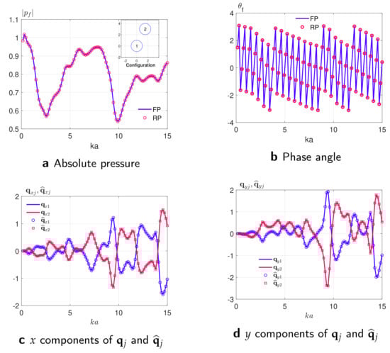
Figure 4. Variation of absolute pressure $p_f$ and phase angle ${\theta }_f$ at a focal point, and the gradient vector components $q_{xj}$${\widehat{q}}_{xj}$, $q_{yj}$ and ${\widehat{q}}_{yj}$ versus a non–dimensional wavenumber $ka$ for FR and RP formulations. The absolute pressure $p_f$ and phase angle ${\theta }_f$ at a focal point, i.e., $\left(10a,0\right)$, and the gradients are computed for a non–symmetric configuration of two cylinders as depicted in top right corner of panel (a).

Figure 5. Absolute pressure at a focal point, i.e., $\left(10a,0\right)$, with respect to normalized wavenumber $ka$ and angle of incidence $\psi$ for configurations that are symmetric (a–c) and non–symmetric (d–f) with respect to the x and y axes.

2.6.2. CPU Timing

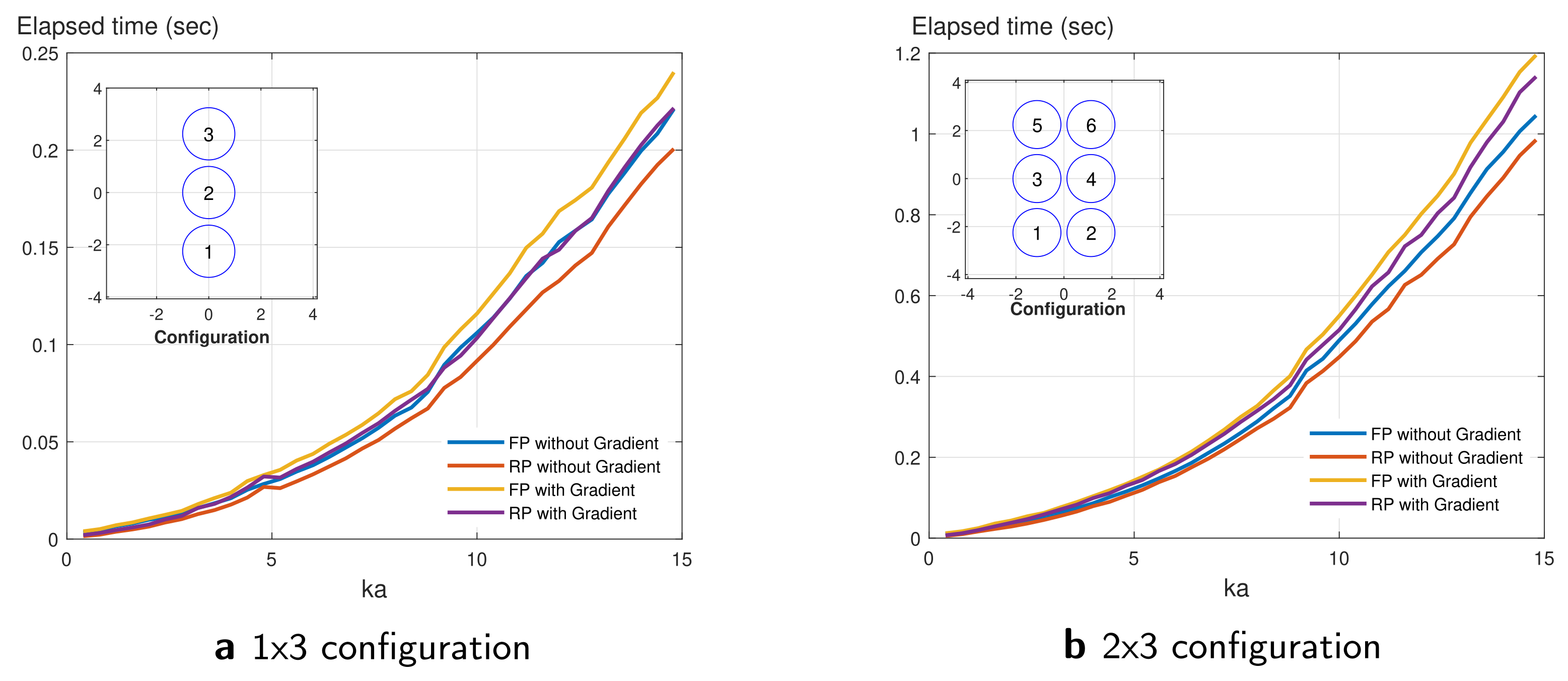
In order to compare between the CPU time of the two computing methods, two configurations were used as depicted in Figure 6a,b. Figure 6 shows the measured time. The elapsed times were used in computing the absolute pressure only, and the absolute pressure and the gradients sequentially varying the wavenumber $ka$ and using both the FP and the RP methods were measured. This was done at different discrete values of $ka\in \left(0,15\right]$. It can be seen from Figure 6 that the computation time generally increases for all computations as the non-dimensional frequency increases. Furthermore, generally the computation time in the configuration with higher number of cylinders is higher. This is due to the increase in the rank of the matrices to be evaluated during the computation process. In addition, the computation time increases for both FP and RP formulations when gradients are evaluated. However, providing gradients improves the performance of GBO algorithms allowing the faster convergence and more accurate and more reliable computations [33]. For $1\times 3$ configuration, FP with gradients takes the most compute time and FP without gradients is the least computation time; the compute times of RP with gradients and FP without gradients are of similar order. For $2\times 3$ configuration, the computation times of different methods can be put in a descending order as follows: FP with gradients, RP with gradients, FP without gradients, and RP without gradients. This depicts that using the RP method is computationally less expensive than the FP method.

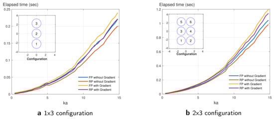
Figure 6. Compute time comparison of FP and RP methods vs. the non–dimensional wavenumber $ka$.

3. Sound Localization by Maximizing the Absolute Pressure at the Focal Point

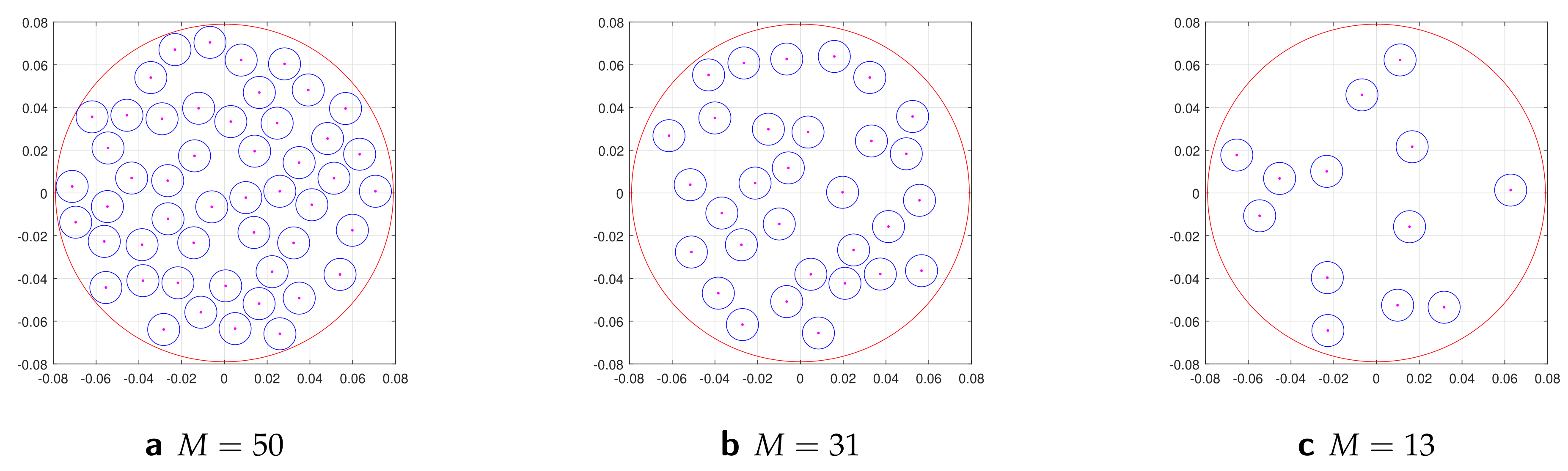
The sound localization was implemented by maximizing the absolute pressure at the focal point and by employing a gradient based optimization. Computations are performed on MATLAB using advanced parallel optimization algorithms, the MultiStart optimization solver combined with fmincon solver and SQP algorithms, and supplying the gradients of absolute pressure amplitude at the focal point $|p_f|$. Figure 7 illustrates initial random configurations of cylinders used in simulation where the locations of the control cylinder positions are denoted by pink dots. For given scatterer location points, the gradients ${\mathbf{q}}_j$ are in the direction of greatest increase of absolute pressure amplitude at the focal point $|p_f|$. As seen in the example of Figure 3 and Figure 4, this provides the optimal directions to increase $|p_f|$ by incremental displacement. Thus, in order to maximize the $|p_f|$ produced by acoustic lens, we will move the cylinders inside the circular region in the direction of the gradient vectors, i.e., ${\mathbf{q}}_j$ using gradients evaluated by FP and RP formulations. This is achieved in MATLAB with the use of Global Optimization and Parallel Computing Toolboxes, and by supplying the derived analytic form of the gradients vectors from Equation (34).

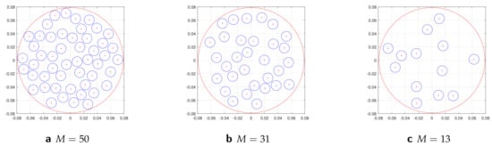
Figure 7. Initial random configurations of $M=13,31,\mathrm{and}50$ cylinders in a circular region considered in numerical simulations. Positions of each scatterer are included as components of feasible initial design vector ${\mathbf{x}}_0^M$ in GBO. The focal point is located at ${\mathbf{x}}_f=(0.0865,0)$. The radius of each cylinder denoted by blue color is $a=0.0075$ m. The radius of artificial red circle is $R=R_{out}+a=0.0715$ m, where $R_{out}=0.0695$ m is defined by constraint Equation (52). This circular region defines the location of acoustic lens comprised of a uniform planar configuration of cylinders constrained to stay within this region.

3.1. Acoustic Lens Design

In order to study the focusing and localization efficiency, we consider three cases: In the first case, we maximize the absolute pressure at a fixed value of frequency and normal incidence while supplying the gradients ${\mathbf{q}}_j$. In the second case, we maximize the root mean square of a set of the absolute pressure over a range of frequencies. In the third case, we maximize the root mean square of a set of the absolute pressure over a range of frequencies and a set of the incident angles of the impinging plane wave. In each case, we supply the analytical formulas for the gradients of objective functions. The cost functions are non-convex with many local maxima. The global maximum is unbounded in each considered cases; we solve the non-convex optimization problems with nonlinear constraints. For simplicity and demonstration of implementation of the proposed approach, we consider a configuration of uniform cylinders/shells of radius a.

3.1.1. Constrained Optimization Problem

The idea is to maximize the absolute pressure at the focal point, $|p_f|$, by rearranging the position of each cylinders and starting with random configuration of scatterers as depicted in Figure 7. The design vector, ${\mathbf{x}}^M$, consist of all scatterer position and can be represented in a column vector form as

$${\mathbf{x}}^M={[{\mathbf{r}}_1,{\mathbf{r}}_2,\dots ,{\mathbf{r}}_M]}^T={[x_1,y_1,x_2,y_2,\dots ,x_M,y_M]}^T,$$

(51)

where M is the total number of scatterers used in lens design. The nonlinear constraints for the design vector components are as follows:

1. The cylindrical scatterers are constrained to move inside a fixed circular region with the radius $r=R_{out}$, see Figure 7:

$$|{\mathbf{r}}_j|<R_{out}$$

(52)

where ${\mathbf{r}}_j=(x_j,y_j)$ and $j=1,2,\dots ,M$.

2. In order to avoid overlapping the distance between the centers of cylinders/shells are constrained by [29]:

$$|{\mathbf{r}}_i-{\mathbf{r}}_j|>2a+\delta ,\mathrm{with}a=0.0075\mathrm{m},\delta =0.0005\mathrm{m}.$$

(53)

As was shown in our earlier work [29] on acoustic cloak design, the closest proximity according to the constraint (53) should be far greater than the viscous skin depth ${\delta }_v={(2\nu /\omega )}^{1/2}$ [42]. In water, at temperature $T=5{}^{\circ }$C with kinematic viscosity $\nu =1.5182$ mm${}^2$/s [43], this is ${\delta }_v=\frac{0.000695m/\sqrt{s}}{\sqrt{f}}$ for frequency f (Hz); therefore, the undamped acoustic model is accurate for frequencies in kHz and above, which is the range of practical interest.

We use direct optimization methods such as SQP algorithms to get the best performance by taking advantage of the analytical form for the gradients of objective functions combined with parallel computing. It is suggested in [33] to include a gradient evaluation in the objective function for faster or more reliable computations. In our computations, we used MATLAB built fmincon solver which is a nonlinear programming solver that finds a local minimum of constrained nonlinear multivariable function. Therefore, to maximize the absolute pressure, we changed the sign of objective function and its gradients.

3.1.2. Broadband Multi-Directional Lens Design

The procedure for a broadband multi-directional GBO is as follows. First, we define the cost function as the root mean square (RMS) of a set of absolute pressure at the focal point $|p_f|$ s over some range of normalized wavenumbers $k_{i}a(i=1,2,\dots ,N_k)$ and over a range of incident angles ${\psi }_l(l=1,2,\dots ,N_l)$:

$$|p_f\left(\left\{{\mathbf{r}}_m\right\}\right){|}^{RMS}={\left(\frac{1}{N_k}\frac{1}{N_{\psi }}\sum _{i=1}^{N_k}\sum _{l=1}^{N_{\psi }}{\left|p_f(k_{i}a,{\psi }_l,\left\{{\mathbf{r}}_m\right\})\right|}^2\right)}^{1/2}.$$

(54)

Then, we define the broadband gradient vectors with respect to positions ${\mathbf{r}}_j$:

$${\mathbf{q}}_j^{RMS}=\frac{\partial |p_f\left(\left\{{\mathbf{r}}_m\right\}\right){|}^{RMS}}{\partial {\mathbf{r}}_j},j=1,2,\dots M,$$

(55)

which can be found in terms of the individual single frequency gradients as

$${\mathbf{q}}_j^{RMS}=\frac{1}{|p_f{|}^{RMS}}\frac{1}{N_k}\frac{1}{N_{\psi }}\sum _{i=1}^{N_k}\sum _{l=1}^{N_{\psi }}\left|p_f(k_{i}a,{\psi }_l,\left\{{\mathbf{r}}_m\right\})\right|{\mathbf{q}}_j(k_{i}a,{\psi }_l),$$

(56)

where $|p_f{|}^{RMS}$ is defined by (54) and ${\mathbf{q}}_j\left(k_{i}a\right)$ are defined by (34) and evaluated at normalized wavenumbers $k_{i}a(i=1,2,\dots ,N_k)$ and angles of incidence ${\psi }_l(l=1,2,...,N_l)$.

For a single angle of incidence ${\psi }_1$, Equations (54) and (56) reduce to the form

$$|p_f\left(\left\{{\mathbf{r}}_m\right\}\right){|}^{RMS}={\left(\frac{1}{N_k}\left[|p_f(k_{1}a,\left\{{\mathbf{r}}_m\right\}){|}^2+|p_f(k_{2}a,\left\{{\mathbf{r}}_m\right\}){|}^2+\dots +{\left|p_f(k_{N_k}a,\left\{{\mathbf{r}}_m\right\})\right|}^2\right]\right)}^{1/2}.$$

(57)

and

$${\mathbf{q}}_j^{RMS}=\frac{1}{|p_f{|}^{RMS}}\frac{1}{N_k}(|p_f\left(k_{1}a\right)|{\mathbf{q}}_j\left(k_{1}a\right)+|p_f\left(k_{2}a\right)|{\mathbf{q}}_j\left(k_{2}a\right)+\dots +|p_f\left(k_{N_k}a\right)|{\mathbf{q}}_j\left(k_{N_k}a\right)).$$

(58)

Both FP and RP formulations allow designing broadband unidirectional lens. Note that a formulation of RP reciprocal problem is given at normal incidence. Therefore, a reciprocal formulation can only be used to design broadband unidirectional lens, whereas a forward formulation can be used in all the cases: a single frequency at single incidence, i.e., unidirectional lens optimized at single frequency; broadband at single incidence, i.e., broadband unidirectional lens; and broadband multi-directional lens designs.

3.2. Numerical Examples of Sound Localization

In this section, the results of the gradient-based optimization of the uni- and multi-directional acoustic lens designs are presented including several performance measures for the frequency and the incidence angle dependencies. The optimized model is an improvement over the initial random configuration of cylinders. Numerical results are demonstrated for configurations of rigid cylinders, cylindrical voids, and empty thin elastic nickel cylindrical shells of thickness $h=0.1a$. We consider cylinders and shells submerged in a medium with the acoustic properties of water: ${\rho }_0=1000$ kg/m${}^3$, $c_0=1480$ m/s. All computations are performed for an incident plane wave propagating from left to right. We illustrate the effect of acoustic lens device on plane wave incidence localized at focal point which resembles the focusing effect of acoustic Luneburg lens.

Various values are taken for the non-dimensional wavenumber, $ka$; the total number of scatterers in the focusing lens, M; the number of discrete frequency points, $N_k$; and the number of discrete incidence angle points $N_l$ for a broadband localization and focusing as defined in Equation (54). Greater accuracy is observed, as expected, with increased number of scatterers M. However, large values of $ka$ and M require longer computation times, and some numerical experimentation is necessary to find the smallest values for which the pressure field can be localized to the desired degree in the acoustic lens.

Numerical computations are performed on MATLAB using parallel optimization algorithms with a MultiStart optimization solver, and supplying the gradients of absolute pressure $|p_f|$ with respect to position vectors. We start with an initial random planar configuration of cylinders or thin shells of uniform size and radius $a=0.0075$ m, e.g., as shown in Figure 7a–e, and consider a focal point located at ${\mathbf{x}}_f=(0.0865,0)$ m. We use MATLAB built function fmincon combined with SQP algorithm and As mentioned in fmincon documentation [33]: “a solver can reach a point x such that x is feasible, but finite differences around x always lead to an infeasible point. In this case, a solver can fail or halt prematurely. Providing a gradient allows a solver to proceed.” Therefore, supplying the gradients accelerates the optimization process by searching a wide variety of start points in parallel and allows the solver to reach the optimum values which may otherwise be impossible [29]. Here, we present results for a ring configuration of M cylinders running 200 different scenarios (initial random configurations) for a single frequency optimization and running 100 scenarios for broadband and multi-incidence-angle optimizations concurrently on 48 CPUs of Dell workstation, described next.

We evaluated the absolute pressure $|p_f{|}_{rel}$ relative to the incident background pressure at the focal point and the magnification factor (MF) defined as

$$|p_f{|}_{rel}=\frac{|p_f|}{|p_{inc}\left({\mathbf{x}}_f\right)|}=\left|p_f\right|\mathrm{and}MF=\frac{|p_f|}{|p_f{|}_{initial}},$$

(59)

where $|p_{inc}\left({\mathbf{x}}_f\right)|$ is the incident plane wave of unit amplitude at the focal point, $|p_f|$ and $|p_f{|}_{initial}$ are correspondingly the absolute pressure at the focal point for the optimized final and initial configurations.

3.2.1. Lens Design at Single Frequency and Normal Incidence

First, we present the localization effect for a plane wave incident on configuration of rigid cylinders depicted in Figure 8 and Figure 9 where various discrete values of normalized wavenumber, $ka$, and the total number of scatterers in acoustic lens, M, were considered. The optimized lens device in each example is a configuration of identical rigid cylinders located inside of circular region of radius $R_{out}=0.0715$ m. Figure 8 shows the real part of total acoustic pressure field p at normal plane wave incidence for a configuration of $M=50$ rigid (or sound hard) cylinder at discrete values of wavenumbers $ka=1,1.5,\mathrm{and}2$. Figure 9 illustrates the absolute total acoustic pressure $\left|p\right|$ for the optimized configurations of $M=13,31,\mathrm{and}50$ cylinders $ka=1,1.5,\mathrm{and}2$. The value of $|p_f|$ and magnification factor, MF, are depicted in Figure 9 for considered values of M and $ka$ under each subfigure.

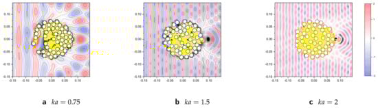
Figure 8. The real part of the total acoustic pressure field p for the optimized configurations of 50 rigid cylinders (a) at $ka=0.75:|p_f{|}_{rel}=\frac{|p_f|}{p_i\left(x_f\right)}=6.43$, (b) $ka=1.5:p_{rel}=4.13$, and (c) $ka=2:p_{rel}=4.62$. For drawing purposes values higher than 2 are denoted by yellow color and values below $-2$ are denoted by dark gray color.

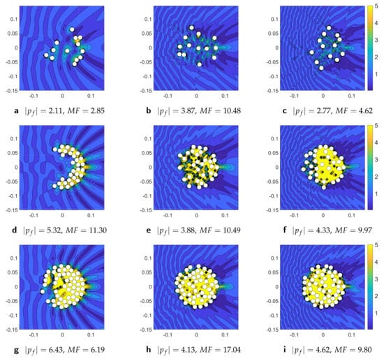
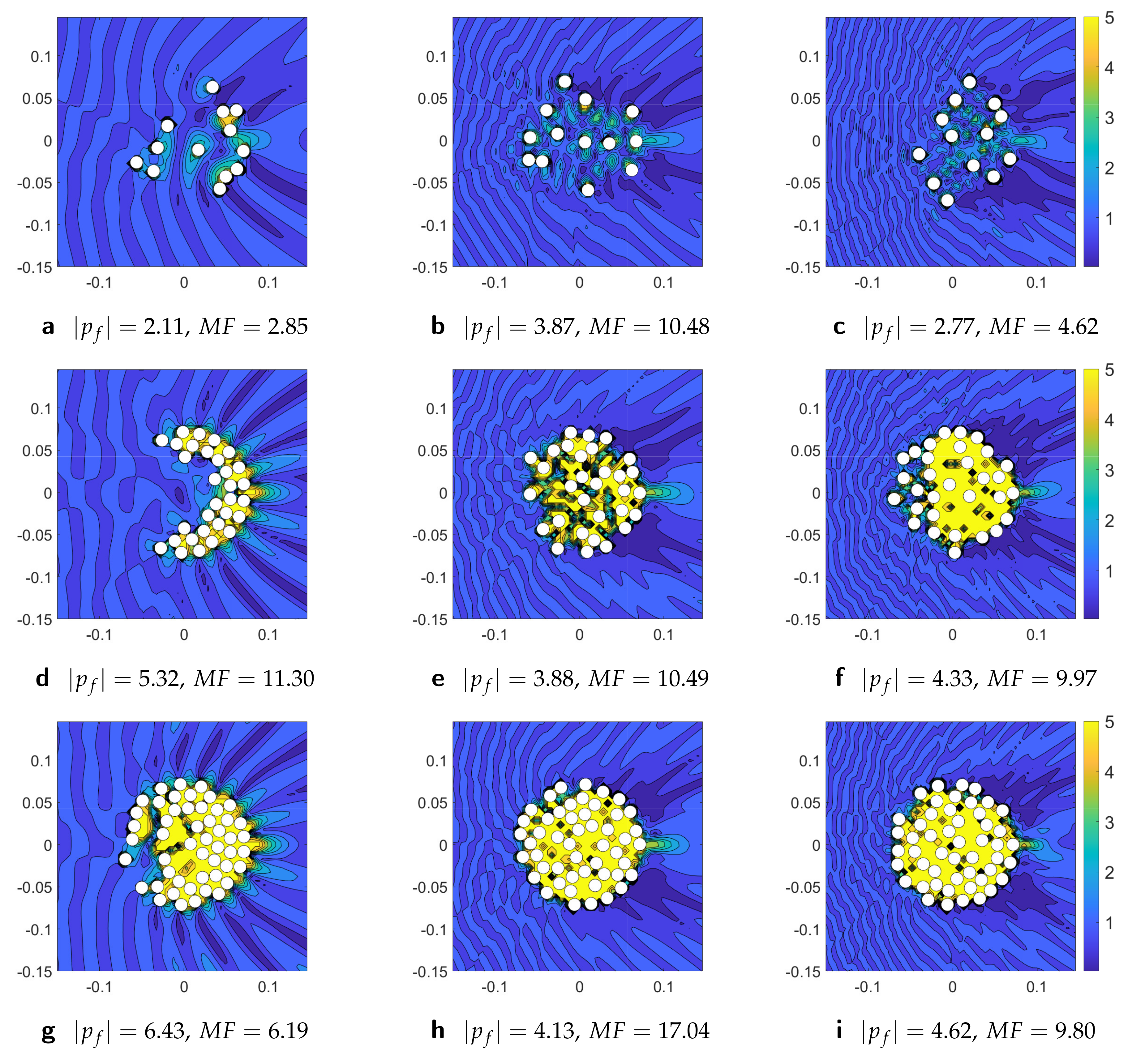
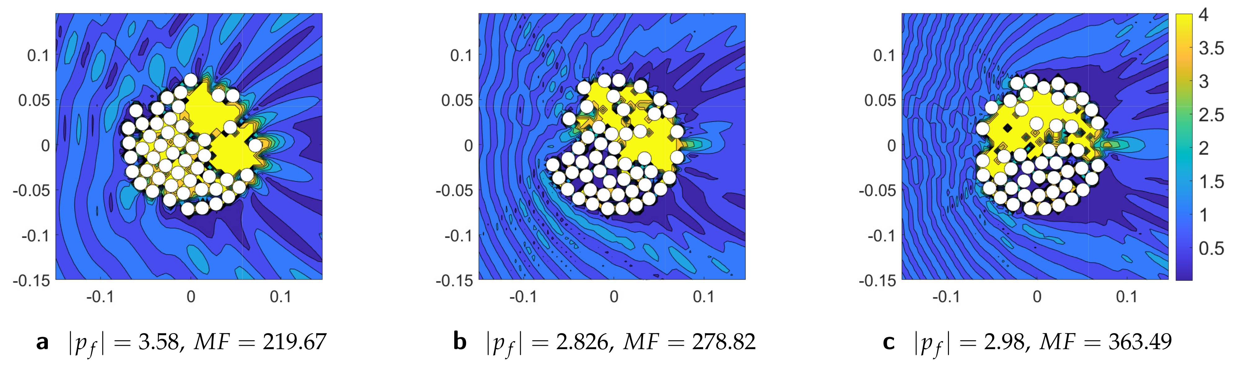
Figure 9. The absolute value of the total acoustic pressure field $\left|p\right|$ at normal plane wave incidence on the optimized configurations of M rigid cylinders at various discrete values of normalized wavenumber, $ka$. The top, middle, and lower rows are for $M=13,31,50$, respectively, and the left, center, and right columns are for $ka=0.75,1.5$, and 2, respectively.

Next, we investigate the sound localization effect for a plane wave incident on configuration of void cylinders considering discrete values of normalized wavenumber, $ka$, and the total number of scatterers in acoustic lens, M. Figure 10 illustrates the absolute total acoustic pressure $\left|p\right|$ computed at normal plane wave incidence for configuration of $M=13,31,\mathrm{and}50$ cylindrical voids (or sound soft cylinders) at normalized wavenumbers $ka=1,1.5,\mathrm{and}2$. The absolute total acoustic pressure $\left|p\right|$ is computed for the optimized configurations of $M=13,31,\mathrm{and}50$ cylinders $ka=1,1.5,\mathrm{and}2$. The value of $|p_f|$ and magnification factor, MF, are depicted in Figure 10 for considered values of M and $ka$ under each subfigure. For $ka=0.75,M=13:|p_f|=22.43,MF=275.35$, the highest amplitude $|p_f|=22.43$ is achieved, and for $ka=2,M=50:|p_f|=2.52,MF=307.27$, the highest values $MF=307.27$ is obtained. The total field results for void cylinders differ both qualitatively and quantitatively from the total field depicted in Figure 9 for rigid cylinders.

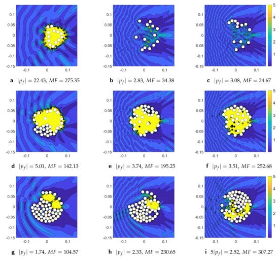
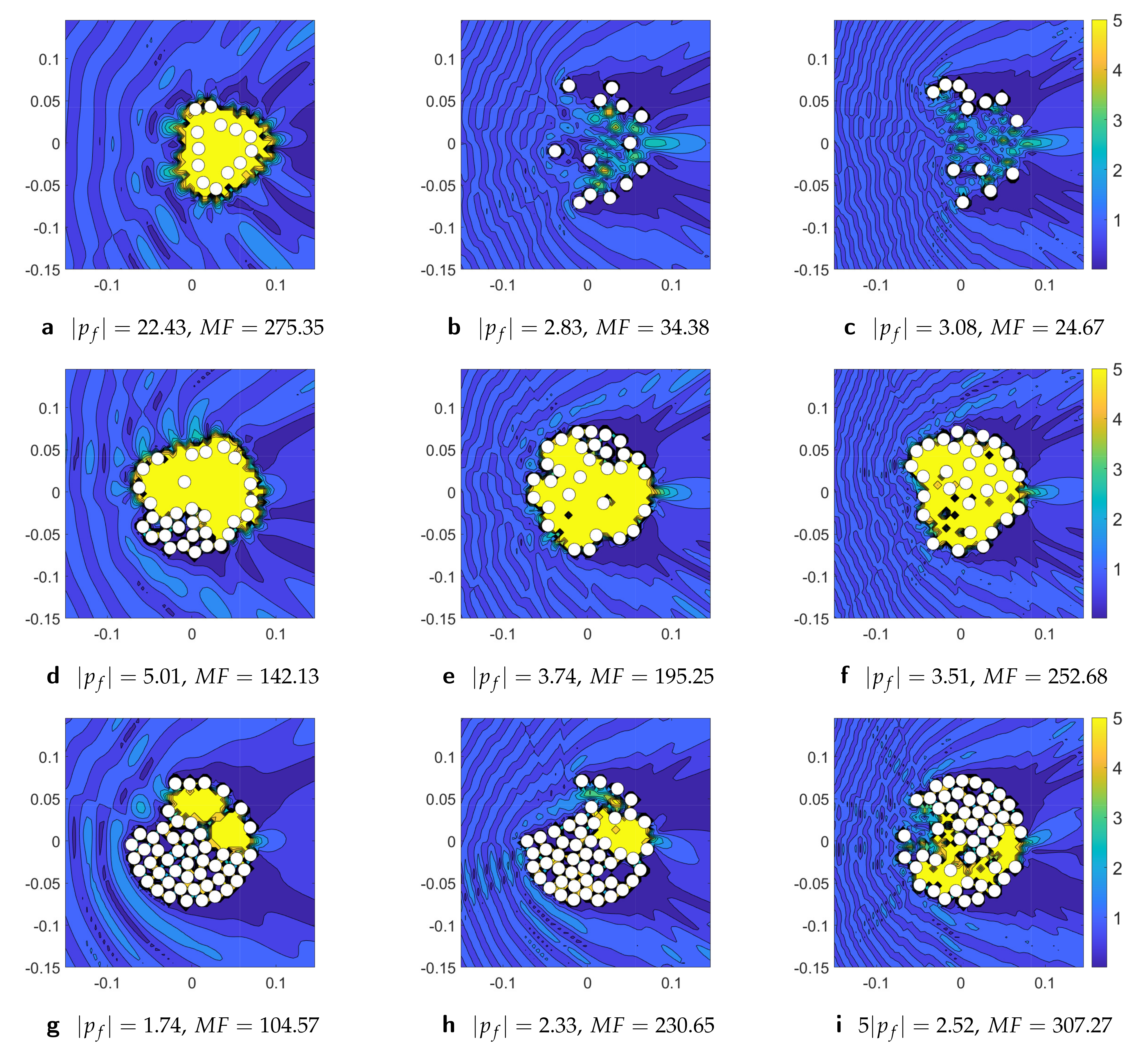
Figure 10. The absolute value of the total acoustic pressure field $\left|p\right|$ for the optimized configurations of M cylindrical voids at normal plane wave incidence from left to right for different fixed values wavenumber $ka$. The top, middle and lower rows are for $M=13,31,50$ voids, respectively, and the left, center, and right columns are for $ka=0.75,1.5$, and 2, respectively.

Finally, we present the sound localization and focusing mechanism for empty elastic thin cylindrical shells submerged in water. We consider empty thin elastic nickel cylindrical shells of thickness $h=0.1a$ with mechanical properties: $\rho =8850$ kg/m${}^3$, $c_p=5480$ m/s where a is the outer radius of scatterer. Figure 11 and Figure 12 illustrate the localization effect for a normal plane wave incident on configurations of elastic thin cylindrical shells at various discrete values of normalized wavenumber, $ka$, and the total number of scatterers M. Figure 11 displays the distribution of absolute total pressure filed $\left|p\right|$ for the optimized configurations of 50 nickel thin cylindrical shells (a) at $ka=0.75$, (b) $ka=1.5$, and (c) $ka=2$. The elastic thin cylindrical shells can display large scattering at low frequency due to internal resonances of longitudinal and flexural waves. This is confirmed by results in Figure 11 (a) at $ka=0.75$, (b) $ka=1.5$, and (c) $ka=2$, showing the highest amplitude for $ka=0.75,M=50:|p_f|=3.5805,MF=219.663$ depicted in Figure 11a. Figure 11 also shows that sound focusing becomes more noticeable with increase of frequencies. Figure 12 exhibits the distribution of absolute pressure field $\left|p\right|$ for the optimized configurations of $M=13,25,31,\mathrm{and}39$ nickel thin cylindrical shells at $ka=1.5$ (top row figures) and $ka=2$ (bottom row figures).

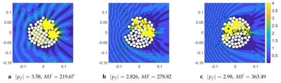
Figure 11. The absolute value of the total acoustic pressure field $\left|p\right|$ for the optimized configurations of $M=50$ nickel thin cylindrical shells at (a) $ka=0.75$, (b) $ka=1.5$, and (c) $ka=2$.

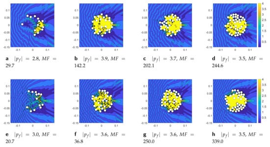
Figure 12. The absolute total acoustic pressure field $\left|p\right|$ for the optimized configurations of $M=13,25,31$, and 39 nickel thin cylindrical shells depicted from the left to the right columns respectively at normalized wavenumbers $ka=1.5$ (the top row figures) and $ka=2$ (the bottom row figures).

It is noticed that, in general, the sound focusing and localization effects are enhanced with the increase of frequency and number of scatterers. The total field distributions for void cylinders and elastic thin shells differ both qualitatively and quantitatively from the total field produced configuration of rigid cylinders. Both void cylinders and elastic thin shells produced high amplification of sound at focal point, i.e., MF values are high, compared to initial configuration. The design can be further improved by considering the cylinder radii as an additional design parameter which will require deriving analytical formulas for the gradients of absolute pressure with respect to cylinder radii and will be studied elsewhere.

3.2.2. Performance of Different Solvers for Lens Design at Single Frequency and Normal Incidence

In this section, we investigate the performance of GBO and GA, compare the best final optimal results produced, and measure the time taken by the optimization functions in all cases. We consider configurations of $M=13$ rigid and elastic scatterers at discreet values of wavenumbers $ka=0.75,1.5,$ and 2 for convenience. For GBO, we first run the fmincon solver with SQP algorithms and then we implement MultiStart optimization combined with fmincon and SQP algorithms. In GBO, we start each time with the feasible design vector ${\mathbf{x}}_0^M$, i.e., the initial random configuration depicted in Figure 7c, and use the central difference for finite differences.

For GA, we solve the optimization problem by running ga solver from Global Optimization Toolbox on MATLAB. The ga solver starts with its own initial random population and we use “rng default” option for reproducibility, analysis and testing of numerical results. We analyze the results for running the ga solver by evaluating fitness functions in parallel using 48 workers (CPUs) concurrently. We keep the maximum number of iterations before the algorithm halts at default option [44], i.e., $MaxGenerations=100\ast 2M=2600$ and vary $MaxStallGenerations$ option to obtain finer solutions. The MathWorks documentation [44] indicates that the $MaxGenerations$ option determines the maximum number of generations that the ga takes and $MaxStallGenerations$ option controls the number of steps the ga looks over to see if it is making progress and can enable the solver to obtain a better solution by allowing more function evaluations. We observed that running the ga solver with above mentioned options, the nonlinear constraints (53) were not always satisfied, the (52) constraints were slightly violated in each of considered cases.

Numerical simulations presented in Table 1 through Table 6 are performed on MATLAB using Dell Workstation with 48 CPUs. In each case, the first column represents the best values of absolute pressure $|p_f|$ obtained by a solver and the second column shows the corresponding elapsed time to compute the optimal values. The elapsed compute time is given in seconds. Table 1 through Table 3 compares the results of fmincon, MultiStart, and ga solver runs for configurations of $M=13$ rigid cylinders. Table 1 depicts the results produced by fmincon with three different options, namely, running fmincon without (w/o) gradients sequentially and in parallel using concurrently 48 workers (CPUs), and running fmincon with gradients sequentially. The results presented show that running fmincon without (w/o) gradients sequentially take 5 to 16 times longer time compared to running fmincon with gradients sequentially. Parallel computing allows to reduce compute time approximately to 3.5 to 7 times. Produced optimal values vary with change of wavenumber. For $ka=0.75$ fmincon with gradients produced better results and for $ka=1.5$ and 2 fmincon without gradients yield higher optimal values.

Table 1. The comparison of results for configuration of $M=13$ rigid cylinders at $ka=0.75,1.5,$ and 2 using fmincon solver with three different options: running fmincon without (w/o) gradients sequentially and in parallel using concurrently 48 workers, and running fmincon with gradients sequentially. The total elapsed compute time is given in seconds.

	Fmincon w/o Gradients, Sequential		Fmincon w/o Gradients, Parallel		Fmincon with Gradients, Sequential
	Optimal Value	Compute Time (s)	Optimal Value	Compute Time (s)	Optimal Value	Compute Time (s)
ka = 0.75	1.8378	192.342	1.8378	27.6712	1.8422	31.3297
ka = 1.5	2.5533	964.727	2.5533	263.194	2.0074	41.734
ka = 2	2.3017	869.472	2.3017	108.144	2.1219	126.185

When analytically evaluated gradients are supplied to fmincon, we can run MultiStart in parallel considering different scenarios concurrently. Table 2 illustrates results for GBO using MultiStart combined with fmincon and SQP algorithms. We run $20,48$, and 200 parallel scenarios with MultiStart using 48 workers concurrently, and providing gradients to fmincon which runs sequentially for each scenario. Considering 20 scenarios, MultiStart already outperforms single fmincon run results shown in Table 1 producing higher optimal values in similar compute times. Increasing the number of scenarios improves the optimal value produced by MultiStart.

Table 2. The comparison of GBO results using MultiStart combined with fmincon and SQP algorithms for the configuration of $M=13$ rigid cylinders at $ka=0.75,1.5,2$. The MultiStart solver results are presented running $20,48$, and 200 parallel scenarios using concurrently 48 workers, and providing gradients to fmincon which run sequentially for each scenario/configuration.

	20 Starting Initial Configurations		48 Starting Initial Configurations		200 Starting Initial Configurations
	Optimal Value	Compute Time (s)	Optimal Value	Compute Time (s)	Optimal Value	Compute Time (s)
ka = 0.75	2.1362	55.9269 s	2.171	239.262 s	2.379	1389.29 s
ka = 1.5	2.8136	940.251 s	2.9287	399.456 s	3.0146	2059.43 s
ka = 2	2.7468	132.335 s	−2.7962	324.068 s	2.82	2960.97 s

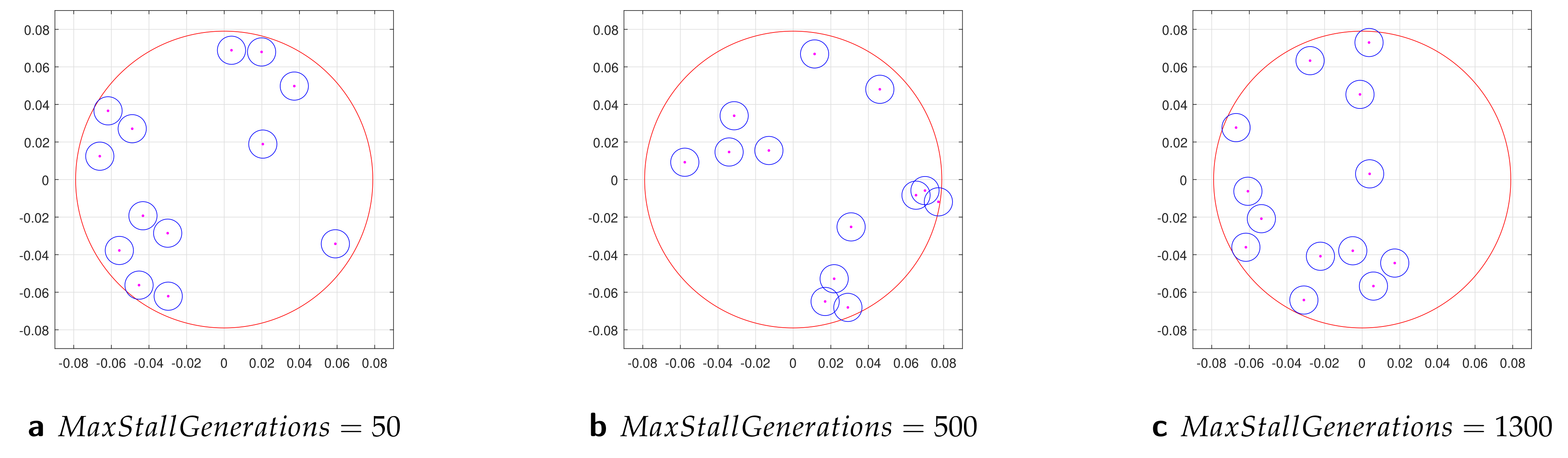
Table 3 shows the results for running ga solver in parallel using concurrently 48 workers with three different options: $MaxStallGenerations=50,500$, and 1300. The ga produced poorer results and took longer to find the best results. The ga solver violated nonlinear constraints (52), although it is still acceptable as predicted optimal scatterer positions are not more one cylinder radii away from constrained circular region $R_{out}$. However, for $ka=0.75$, running ga solver with $MaxStallGenerations=50$ resulted in infeasible solution violating both (52) and (53) constraints and allowing cylinders to overlap. Figure 13 depicts the final scatterer configurations obtained by ga solver for $ka=0.75$ with three different options: $MaxStallGenerations=50$ (a), 500 (b), and 1300 (c). For $MaxStallGenerations=500$, both constraints (52) and (53) are violated, and for $MaxStallGenerations=50$ and 1300 the constraints (52) are slightly violated. The results show that ga struggles to solve the non-convex optimization problem with nonlinear constraints.

Table 3. The comparison of results for configuration of $M=13$ rigid cylinders at $ka=0.75,1.5,2$ running ga solver in parallel using concurrently 48 workers with three different options: $MaxStallGenerations=50,500$, and 1300. In each case, the constraints (52) are slightly violated and in some cases predicted final cylinder positions are up to one cylinder radii away from a circular region of radius $R_{out}$. At $ka=0.75$, ga with option $MaxStallGenerations=500$ produces an infeasible solution violating both (52) and (53) constraints.

	$\mathit{MaxStallGenerations}=50$		$\mathit{MaxStallGenerations}=500$		$\mathit{MaxStallGenerations}=1300$
	Optimal Value	Compute Time (s)	Optimal Value	Compute Time (s)	Optimal Value	Compute Time (s)
ka = 0.75	0.74158	140.505	Equations (52) and (53) violated		0.33408	730.226
ka = 1.5	0.29781	290.763	0.30743	0.30743	0.69264	1599.15
ka = 2	0.67394	419.28	0.74616	1520.26	0.27124	1826

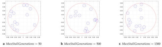
Figure 13. Final configurations of $M=13$ rigid cylinders obtained by ga solver for $ka=0.75$ with three different options: $MaxStallGenerations=50$ (a) producing $|p_f{|}_{opt}=0.74158$, $MaxStallGenerations=500$ (b) producing infeasible solution, and $MaxStallGenerations=1300$ (c) yielding $|p_f{|}_{opt}=0.33408$. The focal point is located at ${\mathbf{x}}_f=(0.0865,0)$. The radius of each cylinder denoted by blue color is $a=0.0075$ m. The radius of artificial red circle is $R=R_{out}+a=0.0715$ m where $R_{out}=0.0695$ m is defined by constraint Equation (52). For $MaxStallGenerations=500$, both constraints (52) and (53) are violated. For $MaxStallGenerations=50$ and 1300, the constraints (52) are slightly refused to confirm but most of cylinders are located inside of predefined circular region and we may consider the configurations in subfigures (a,c) as acceptable.

Table 4, Table 5 and Table 6 analyze the results of fmincon, MultiStart, and ga solver runs for configurations of $M=13$ thin elastic shells with the same options used for the configurations of rigid scatterers presented above in Table 1 through Table 3. Analyzing parallel runs of fmincon w/o gradients and MultiStart runs starting with 20 scenarios indicate that MultiStart produced much more enhanced results within a comparable compute time. In addition, the MultiStart solver starting from 200 various random configurations yields the best results and outperforms fmincon solver with and without providing gradients as well as the ga solver. The ga solver running with parallel option performs much poorer producing much lower values of $|p_f|$ and violating constraints (52). Increasing $MaxStallGenerations$ option values with ga solver overall has tendency to obtain more improved results but also required longer compute times from 3 to 6 times.

Table 4. The comparison of results for configuration of $M=13$ thin elastic shells at $ka=0.75,1.5,2$ using fmincon solver with three different options: running fmincon without (w/o) gradients sequentially and in parallel using concurrently 48 workers, and running fmincon with gradients sequentially.

	Fmincon w/o Gradients, Sequential		Fmincon w/o Gradients, Parallel		Fmincon with Gradients, Sequential
	Optimal Value	Compute Time (s)	Optimal Value	Compute Time (s)	Optimal Value	Compute Time (s)
ka = 0.75	4.2174	1127.56	4.217	144.86	1.5457	9.17429
ka = 1.5	2.0025	2030.35	2.0025	319.993	2.4193	43.9729
ka = 2	2.5211	567.85	2.521	87.4303	2.553	69.972

Table 5. The comparison of GBO results using MultiStart combined with fmincon and SQP algorithms for the configuration of $M=13$ thin elastic shells cylinders at $ka=0.75,1.5,2$. The MultiStart solver results are presented running $20,48$, and 200 parallel scenarios using concurrently 48 workers, and providing gradients to fmincon which run sequentially for each scenario/configuration.

	20 Starting Initial Configurations		48 Starting Initial Configurations		200 Starting Initial Configurations
	Optimal Value	Compute Time (s)	Optimal Value	Compute Time (s)	Optimal Value	Compute Time (s)
ka = 0.75	6.145	230.028	6.1941	479.538	6.5252	625.877
ka = 1.5	2.7405	246.051	2.8432	391.008	2.884	3084.25
ka = 2	2.9388	410.131	2.869	2539.28	2.9718	1880.6

Table 6. The comparison of results for a configuration of $M=13$ elastic thin cylindrical shells at $ka=0.75,1.5,2$ running ga solver in parallel using concurrently 48 workers with three different options: $MaxStallGenerations=50,500$, and 1300.

	$\mathit{MaxStallGenerations}=50$		$\mathit{MaxStallGenerations}=500$		$\mathit{MaxStallGenerations}=1300$
	Optimal Value	Compute Time (s)	Optimal Value	Compute Time (s)	Optimal Value	Compute Time (s)
ka = 0.75	0.052956	114.204	0.32069	530.695	0.51462	762.944
ka = 1.5	0.19884	543.15	1.2581	627.457	0.13304	1316.46
ka = 2	0.19951	208.066	0.074332	881.275	0.52169	1784.5

The GBO results illustrated in this section show the advantages of using MultiStart with fmincon which produced the highest values of absolute pressure $|p_f|$ when combined with parallel computing. The difference becomes more noticeable with the increase of number of scatterers and wavenumber. We observed that MultiStart integrated with fmincon supplying gradients was able to converge and obtain optimal solutions for configurations with larger number of scatterers and high frequencies for which single fmincon runs without supplying gradients were not able to converge and/or to obtain optimal values in reasonable time.

3.2.3. Broadband Design of Uni- and Multi-Directional Acoustic Lens

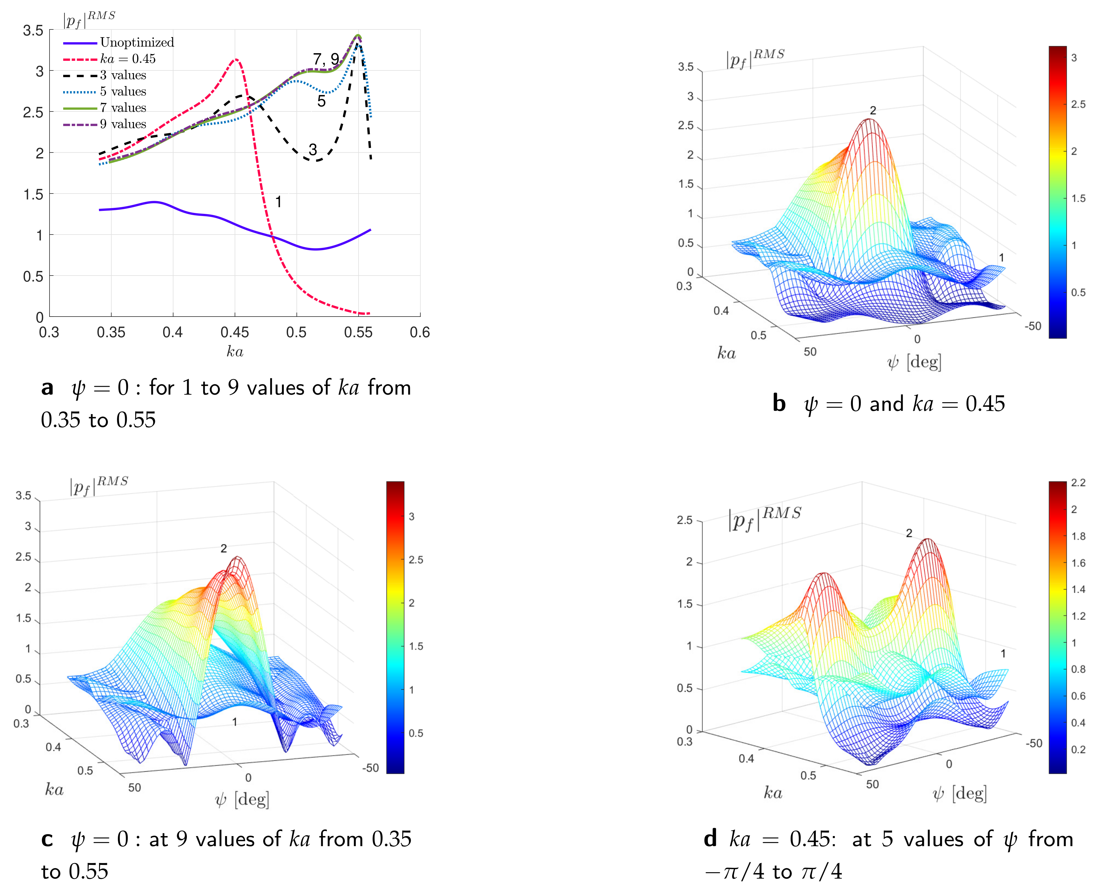
Figure 14 through Figure 18 illustrate the broadband focusing performance of unidirectional and multi-directional lens. We optimize the RMS of absolute pressure amplitude at the focal point, $|p_f{|}^{RMS}$, defined by Equation (54) for given sets of normalized wavenumbers $(N_k=\overline{1,9})$ and incident angles $(N_l=\overline{1,5})$ while supplying the analytical form of gradients ${\mathbf{q}}_j^{RMS}$ given by Equation (56). Figure 14 exhibits the dependency of the objective function $|p_f^{RMS}|$ on the normalized wavenumber $ka$ and on the angle of the incident plane wave $\psi$ for the optimized and initial unoptimized configurations of $M=50$ rigid cylinders. The RMS of absolute pressure at focal point $|p_f{|}^{RMS}$ is maximized at 1, 3, 5, 7, and 9 equidistant values of wavenumber $ka\in [0.35,0.55]$ at normal incidence $\psi =0$. Figure 14a displays the variation of $|p_f{|}^{RMS}$ with wavenumber $ka$ for unoptimized initial random and optimized configurations with $N_k=1,3,5,7,9$ equidistant values of $ka$ in the interval $0.35\le ka\le 0.55$ which corresponds to frequencies from 11 kHz to 17,274 Hz. Figure 14b–d illustrates the dependency of the objective function $|p_f^{RMS}|$ on $ka$ and $\psi$ simultaneously via 3D parametric surface plots. Here, the lower blue mesh denoted by “1” represents the results for a non-optimized configuration and the higher mesh indicated by “2” exhibits the results for the configuration optimized. The results in Figure 14b–d for the non-optimized configurations “1” show overall low values of $|p_f{|}^{RMS}$ in comparison to the mesh surface plots for optimized configurations “2” as illustrated; the results for “2” show clearly the amplification of $|p_f^{RMS}|$. For the fixed value $ka=0.45$, the surface plots in Figure 14d show that the optimized configuration “2” produces the peak performance $ka=0.45$ and near the incidence angles $-\pi /4$ and $\pi /4$; the surface plot “2” produced lower values of $|p_f^{RMS}|$ at wavenumbers near $ka=0.55$ for all $\psi$ values considered which also coincides with results in Figure 14a, denoted by the red curve “1”. The trade-off between the increase of the frequency band and focusing efficiency leads to shift of peak performance for broadband focusing achieving the maximum performance at $ka=0.55$ which is not intuitive.

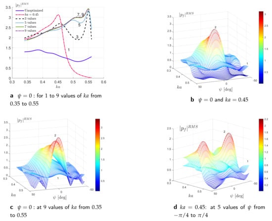
Figure 14. The RMS of pressure at focal point, $|p_f{|}^{RMS}$, optimized at 1, 3, 5, 7, and 9 equidistant values of wavenumber $ka\in [0.35,0.55]$ for the optimized configurations of $M=50$ rigid cylinders at $\psi =0$ and $\psi \in [-\pi /4,\pi /4]$. In subfigures (b–d), “1” denotes results for non–optimized configuration and “2” represents results for optimized configuration.

Figure 15 illustrates the performance of broadband unidirectional lens at different values wavenumbers $ka$ and displays the distribution of absolute total acoustic pressure field $\left|p\right|$ for the optimized unidirectional lens, the configuration of $M=50$ rigid cylindrical scatterers. The top row of Figure 15 shows results for the absolute pressure $\left|p\right|$ for values of wavenumber $ka$ at which the lens was optimized, i.e., (a) $ka=0.35$, (b) $ka=0.45$, and (c) $ka=0.55$. The bottom row of Figure 15 displays the absolute total field for values of $ka$ at which the lens was not optimized, i.e., (d) $ka=0.225$, (e) $ka=0.4$, and (f) $ka=0.585$. Figure 15a–c clearly shows the focusing effect. Figure 15d,f illustrates that focusing amplitudes reduces, and beyond these values, i.e., $0<ka\le 0.225$ and $ka>0.585$, the focusing effect diminishes. Importantly, Figure 15e exhibits clearly the sound localization at the desired focal region at wavenumber $ka=0.4$ at which the configuration was not optimized.

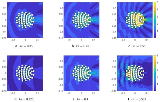
Figure 15. The absolute value of the total acoustic pressure field $\left|p\right|$ for the optimized unidirectional lens, the configuration of $M=50$ rigid cylindrical scatterers at different values of wavenumber $ka$. The unidirectional lens is optimized for $ka=0.35,0.45,\mathrm{and}0.55$, and ${\mathbf{x}}_f=(0.0865,0)$ and the performance is shown at these values of $ka$ (the top row figures) and beyond this range (the bottom row figures).

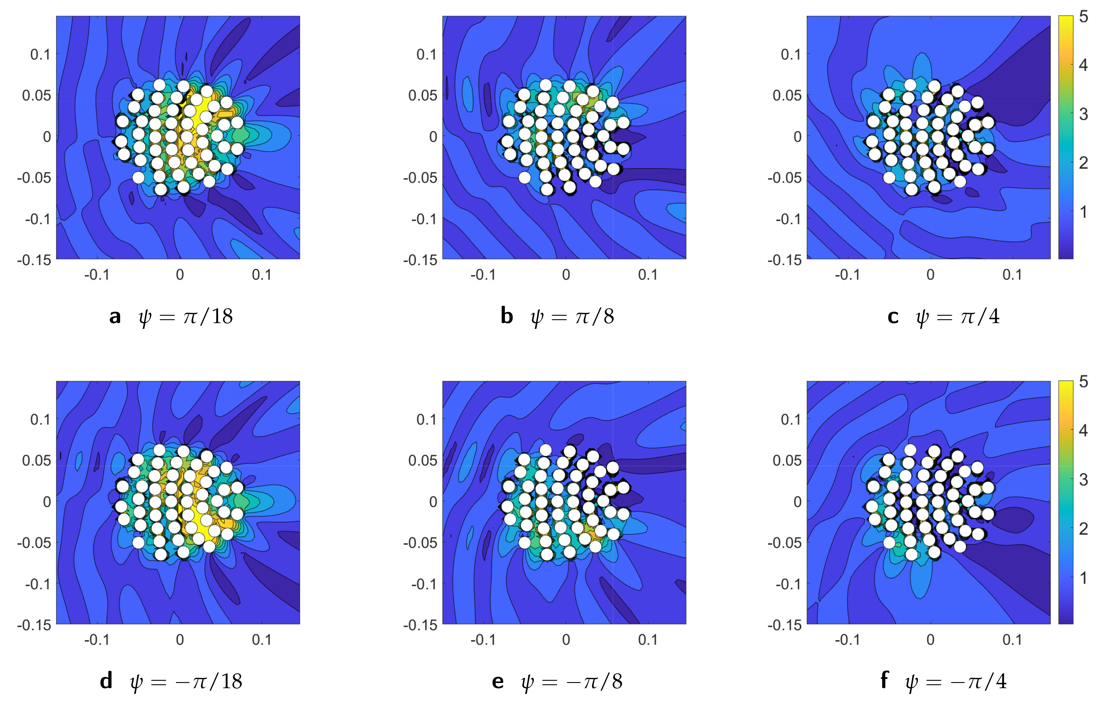
Figure 16 displays the distribution of absolute total acoustic pressure field $\left|p\right|$ for the optimized unidirectional lens, the configuration of $M=50$ rigid cylindrical scatterers at $ka=0.55$ varying values of incident angle $\psi$. The unidirectional lens is optimized for $ka=0.35,0.45,\mathrm{and}0.55$ at normal incidence, i.e., $\psi$, and the performance is shown at angles of incidence $\psi =\pi /18,\pi /8,\pi /4,\pi /18,-\pi /8,-\pi /4$. The unidirectional lens is able to localize the sound well at normal incidence and at small incident angles $\psi =\pm \pi /18$ and with increase of $\psi$ angle values focusing effect deteriorates.

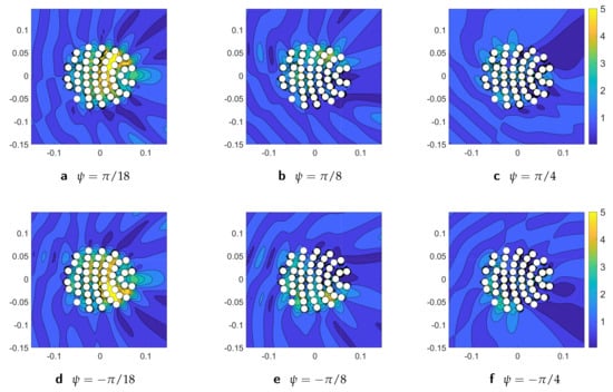
Figure 16. The absolute value of the total acoustic pressure field $\left|p\right|$ for the unidirectional lens optimized at normal incidence, i.e., the configuration of $M=50$ rigid cylinders at wavenumber $ka=0.55$ and different angles of incidence $\psi$. The performance of optimized unidirectional lens at normal incidence, i.e., $\psi =0$, is depicted in Figure 15c.

Figure 17 presents $|p_f{|}^{RMS}$, as a function of incidence angle and the normalized wavenumber $ka$ considering a simultaneous multi-frequency and multi-angle optimization of $|p_f{|}^{RMS}$ at a broad range of the incidence angle $\psi \in [-\pi /4,\pi /4]$ and 3 values of wavenumber $ka$ for configurations of $M=50$ rigid cylinders. Figure 17a–c displays the variation of $|p_f{|}^{RMS}$ with the angle of incidence at three fixed values of wavenumber $ka=0.35$ (a), $ka=0.45$ (b), and $ka=0.55$ (c) for the optimized and initial unoptimized configurations cylinders. Figure 17d illustrates the 3D surface plot of $|p_f^{RMS}|$ versus $ka$ and $\psi$ simultaneously. Here, the lower blue mesh denoted by “1” represents the results for a non-optimized configuration and the higher mesh indicated by “2” exhibits the results for the configuration optimized at three values of wavenumbers and five incident angles. Figure 17d shows that the non-optimized surface mesh “1” depicts the low values of $|p_f^{RMS}|$ in all considered values of $ka$ and $\psi$, and the surface mesh “2” is slightly lifted up with its highest amplification around $\psi =-\pi /4$ and $\psi =\pi /4$ at the largest values of $ka$ considered, i.e., $ka=0.55$. As can be seen from these figures, optimizing $|p_f{|}^{RMS}$ for angle of incidence $\psi \in [-\pi /4,\pi /4]$ using five equidistant values of $\psi$, the overall $|p_f^{RMS}|$ show low values in the incidence range considered which suggests that this range is too ambitious for the small number of discrete incident angles and frequencies considered. Therefore, we narrow it down to $\psi \in [-\pi /8,\pi /8]$.

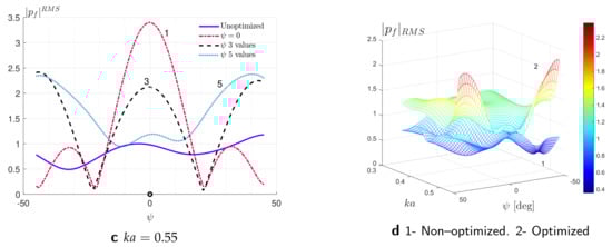
Figure 17. The RMS of pressure at focal point, $|p_f{|}^{RMS}$, optimized at 3 values of $ka=0.35,0.45,0.55$ and 5 equidistant values of $\psi \in [-\pi /4,\pi /4]$ for the optimized configurations of $M=50$ rigid cylinders. In (d), “1” denotes the results for a non–optimized configuration and “2” represents the results for the optimized configuration.

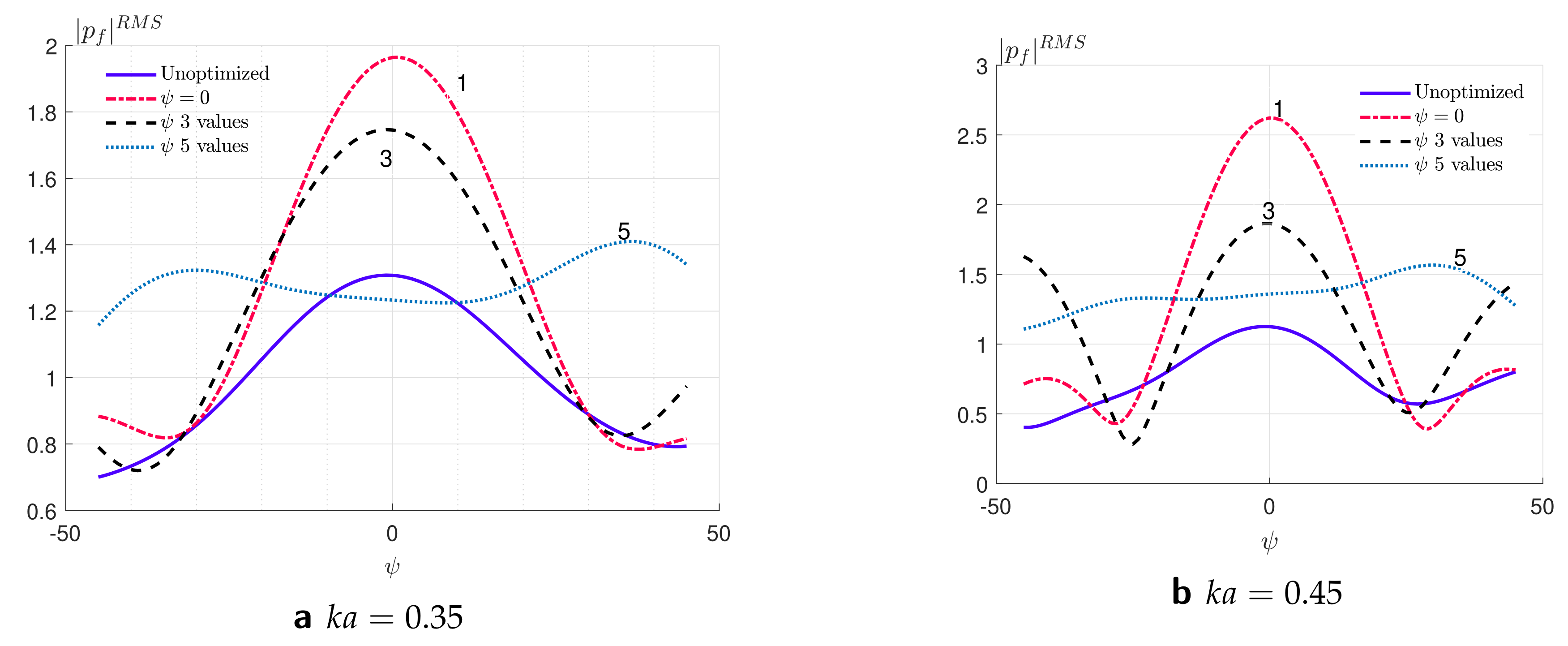
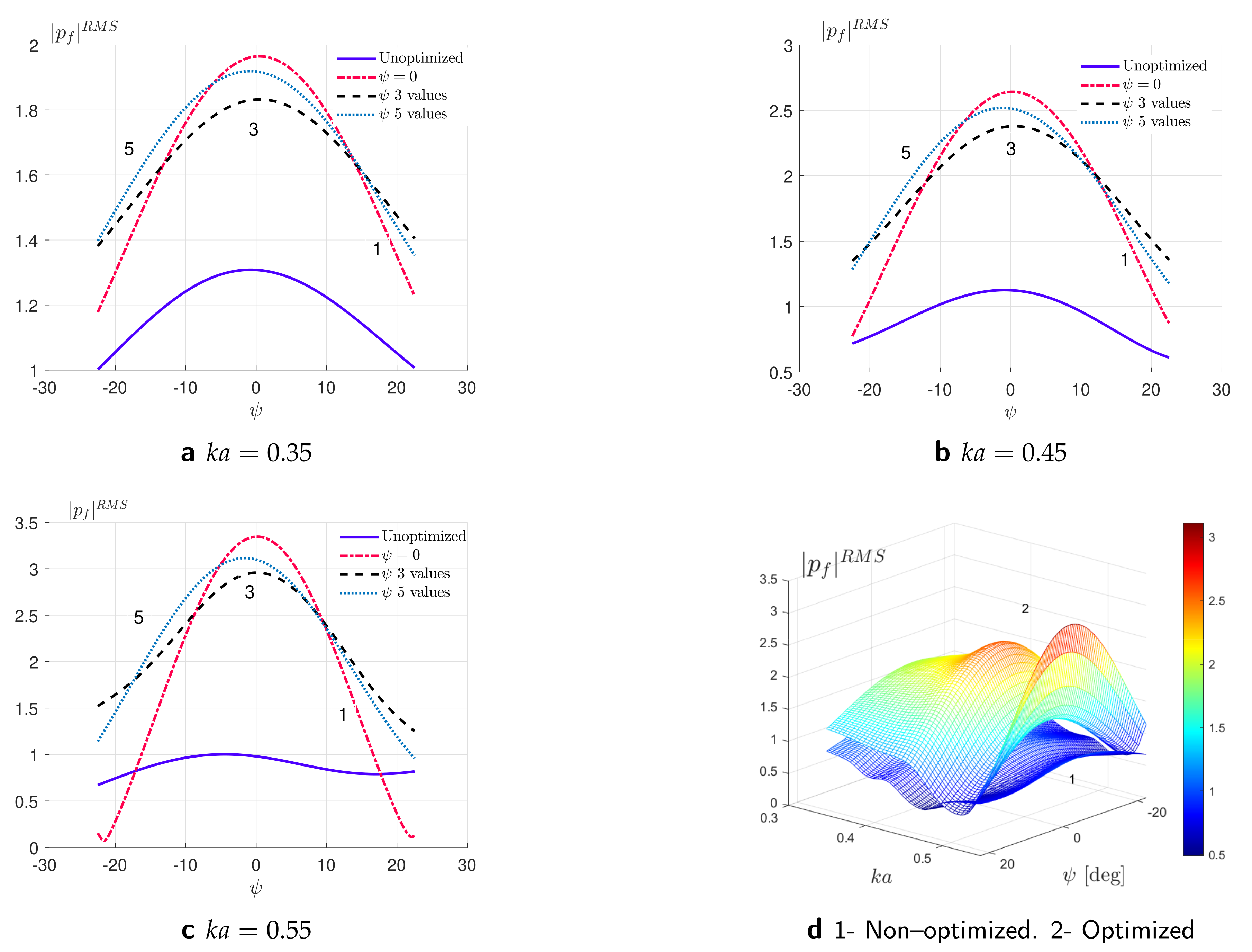
Figure 18 exhibits the distribution of RMS of the absolute pressure amplitude at focal point, $|p_f{|}^{RMS}$, optimized at three values of $ka=0.35,0.45,0.55$ and at three and five equidistant values of $\psi \in [-\pi /8,\pi /8]$ for the optimized configurations of $M=50$ rigid cylinders. The results for an unoptimized initial random configuration depicted in Figure 7a are included as a reference. Figure 18a through Figure 18c present correspondingly the variation of RMS of the absolute pressure amplitude at focal point, $|p_f{|}^{RMS}$ with respect to the angle of incidence at 3 fixed values of wavenumber $ka=0.35$ (a), $ka=0.45$ (b), and $ka=0.55$ (c). Here, the red-dashed curve corresponds to configuration optimized at single value of $\psi =0$ corresponding to normal incidence and the solid blue curve mean results for an unoptimized initial configuration at normal incidence. Figure 18a–c shows that adding more angles of incidence as a parameter in optimization broadens the range of application of multi-directional acoustic lens and improves its performance. Although optimizing at three values of $\psi =-\pi /8,0,\pi /8]$ shifted up $|p_f{|}^{RMS}$ at edge values $\psi =-\pi /8$ and $\psi =\pi /8]$, it reduced the peak at $\psi =0$. The peak performance at $\psi =0$ was further enhanced by optimizing $|p_f{|}^{RMS}$ at five equidistant values of $\psi \in [-\pi /8,\pi /8]$ across all three values of $ka$ as can be seen from these figures. Figure 18d illustrates the dependency of the objective function $|p_f^{RMS}|$ on $ka$ and $\psi$ simultaneously via 3D parametric surface plots. Here, the lower blue mesh denoted by “1” represents the results for a non-optimized configuration and the higher mesh indicated by “2” exhibits the results for the configuration optimized at three values of wavenumber $ka$ and at five equidistant values of incident angles $\psi \in [-\pi /8,\pi /8]$. In comparison to Figure 17d, the results in Figure 18 show better performance of GBO algorithm to produce a broadband multi-incident sound localization effect. The optimized design illustrates broadband performance as compared to initial configuration response although it is not included as an optimization criterion.

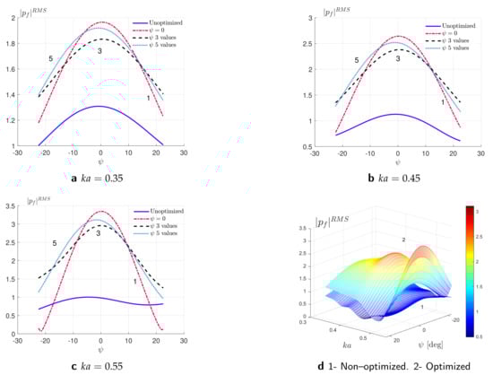
Figure 18. The RMS of the pressure at focal point, $|p_f{|}^{RMS}$, optimized at 3 values of $ka=0.35,0.45,0.55$ and at 5 equidistant values of $\psi \in [-\pi /8,\pi /8]$ for the optimized configurations of $M=50$ rigid cylinders. In panel (d), “1” denotes the results for a non–optimized configuration and “2” represents the results for the optimized configuration.

We notice that the trade-off between the increase of range of incidence and focusing efficiency leads to reduced peak performance for simultaneous broad-range incidence and broadband focusing. Results in Figure 17 for broader incidence angle range $\psi \in [-\pi /4,\pi /4]$ are poorer compared to range $\psi \in [-\pi /8,\pi /8]$ given in Figure 18. The results for a broader range of $\psi$, i.e., $\psi \in [-\pi /4,\pi /4]$, can be improved increasing the number of incidence angles in RMS computation, considering non-equidistant values of $\psi$, and choosing more points (angles) around region where $|p_f{|}^{RMS}$ values are the lowest.

4. Conclusions

We have demonstrated that the GBO technique combined with the principle of acoustic reciprocity leads to an effective method to optimally arrange scatterers so as to produce acoustic focusing. The approach uses semi-analytic expressions for the gradient of the focal pressure with respect to the scatterer positions. Two problem formulations have been considered for the inverse design of the acoustic lens: forward and reciprocal. A comparison of simulation times for both formulations shows that the reciprocal formulation takes less time to compute the absolute pressure and its gradients at the focal point. The specific type of acoustic lens considered consists of a meta-cluster of rigid cylinders or cylindrical voids or thin elastic shells submerged in water. The computations were performed using advanced parallel optimization algorithms on MATLAB, a MultiStart optimization solver, and semi-analytic expressions for the gradient of pressure at the focal point. Numerical results for the uni- and multi-directional broadband acoustic lens designs indicate that significant sound pressure amplification can be achieved by optimal scatterer rearrangement using this analytical-numerical technique. The greatest magnification in amplitude is realized using void-like scatterers.

The presented gradient assisted inverse design model provides a means to establish realistic strategies for an acoustic lens device and for its practical underwater applications. The proposed method can be extended to design 3D lenses including air-born sound and underwater acoustic, elastodynamic, or electromagnetic wave localization and focusing effects. The gradient assisted inverse design of acoustic lens can be further enhanced and implemented by integrating the gradient information, i.e., Equation (37) with deep reinforcement learning algorithms [45] and generative networks [46] which have potential to search for the globally optimized devices over a broad range of parameters and can provide better solutions than ones produced by the-state-of-the-art optimization algorithms.

Appendix A.1. Multiple Scattering Theory

Consider acoustic multiple scattering by M obstacles. For simplicity, the obstacles are assumed to be cylinders ${\mathtt{S}}_m,(m=\overline{1,M})$ centered at ${\mathbf{r}}_m$. A schematic configuration of cylindrical elastic shells is given in Figure A1. The incident field in the neighborhood of cylinder ${\mathtt{S}}_m$ is

$$p_{inc}^{\left(m\right)}\left(\mathbf{x}\right)=\sum _{n=-\infty }^{\infty }{A}_n^{\left(m\right)}{U}_n^{+}\left({\mathbf{x}}_m\right),$$

(A1)

where ${\mathbf{x}}_m$ is a position vector of point P with respect to the centers of multipoles at $O_m$ (see Figure A1):

$${\mathbf{x}}_m=\mathbf{x}-{\mathbf{r}}_m,$$

(A2)

the functions $U_n^{\pm }\left(\mathbf{x}\right)$ are

$$U_n^{\pm }\left(\mathbf{x}\right)=J_n\left(k\right|\mathbf{x}\left|\right)e^{\pm inarg\mathbf{x}}.$$

(A3)

Here, $arg\mathbf{x}\in [0,2\pi )$ and $arg(-\mathbf{x})=\left(arg\mathbf{x}\pm \pi \right)mod2\pi$, and $J_n\left(x\right)$ is the Bessel function of the first kind of order n.

Figure A1. A point source impinging on an isotropic multilaminate cylinder submerged in a fluid medium. Note that here $\mathbf{x}-{\mathbf{x}}^{\prime }={\mathbf{x}}_m-{\mathbf{x}}_m^{\prime }$.

In Equation (A1), the unknown coefficients $A_n^{\left(m\right)}$ are for an incident wave of unit amplitude in direction, ${\mathbf{e}}_1=(1,0)$:

$$p^{inc}\left(\mathbf{x}\right)=e^{ik{\mathbf{e}}_1·\mathbf{x}}\Rightarrow A_n^{\left(m\right)}=e^{ik{\mathbf{e}}_1·{\mathbf{r}}_m}{e}^{in\frac{\pi }{2}}=e^{ik{x}_m}{e}^{in\frac{\pi }{2}}.$$

(A4)

In Equation (A1), the unknown coefficients $A_n^{\left(m\right)}$ for a plane wave incidence are derived assuming no source term: $p_S=0$, and that the incident wave is the plane wave of unit amplitude in direction $\psi$:

$$p^{inc}=e^{ik{\mathbf{e}}_{\psi }·\mathbf{x}}\Rightarrow A_n^{\left(m\right)}=e^{ik\widehat{\mathbf{e}}\left(\psi \right)·{\mathbf{r}}_{\mathbf{m}}}{e}^{in(\frac{\pi }{2}-\psi )}=e^{ik(x_{m}cos\psi +y_{m}sin\psi )}{e}^{in(\frac{\pi }{2}-\psi )}.$$

(A5)

A point source normalized by its amplitude at the origin is defined by

$$p^{inc}=A_0{H}_0^{\left(1\right)}\left(k_{\perp }{r}^{\prime }\right)e^{i{k}_{z}z}\mathrm{where}{A}_0=1/H_0^{\left(1\right)}(k_{\perp }|{\mathbf{x}}^{\prime }|),$$

(A6)

and $r^{\prime }=|\mathbf{x}-{\mathbf{x}}^{\prime }|$. For a source at point S depicted in Figure A1, the coefficients $A_n^{\left(m\right)}$ follow from Equation (A6), noting that in the local coordinates of multipole centered at $O_m$:

$$r^{\prime }=|\mathbf{x}-{\mathbf{x}}^{\prime }|=|{\mathbf{x}}_m-{\mathbf{x}}_m^{\prime }|,$$

where ${\mathbf{x}}^{\prime }$ is the position vector of source at point S with respect to origin O, ${\mathbf{x}}_m$ and ${\mathbf{x}}_m^{\prime }$ are correspondingly the position vectors of an arbitrary point P and a source S with respect to $O_m$. Thus, in the neighborhood of cylinders ${\mathtt{S}}_m$, $A_n^{\left(m\right)}$ can be derived as

$$p^{inc}=A_0\sum _{n=-\infty }^{\infty }{U}_n^{+}\left(k{\mathbf{x}}_m\right)V_n^{-}\left(k{\mathbf{x}}_m^{\prime }\right)\Rightarrow A_n^{\left(m\right)}=A_0{V}_n^{-}\left(k{\mathbf{x}}_m^{\prime }\right),$$

(A7)

for $m=\overline{1,M},n\in \mathbb{Z}$, where the Graf’s addition theorem (A10) is used for $|{\mathbf{x}}_m|<|{\mathbf{x}}_m^{\prime }|$ (see Figure 1).

The total scattered field $p_{sc}$, considered as a superposition of the scattered fields by all cylinders, may be expanded as a sum of multipoles:

$$p_{sc}\left(\mathbf{x}\right)=\sum _{m=1}^M{p}_{sc}^{\left(m\right)}\left(\mathbf{x}\right),p_{sc}^{\left(m\right)}\left(\mathbf{x}\right)=\sum _{n=-\infty }^{\infty }{B}_n^{\left(m\right)}{V}_n^{+}\left({\mathbf{x}}_m\right),$$

(A8)

where $p_{sc}^{\left(m\right)}$ is the wave scattered by cylinder ${\mathtt{S}}_m$, $B_n^{\left(m\right)}$ are unknown coefficients, and

$$V_n^{\pm }\left(\mathbf{x}\right)=H_n^{\left(1\right)}\left(k\right|\mathbf{x}\left|\right)e^{\pm inarg\mathbf{x}}.$$

(A9)

In order to use boundary conditions on the surface of each cylinder ${\mathtt{S}}_m$, we will express the total field using Graf’s theorem ([47] Equation (9.1.79)):

$$V_l^{+}(\mathbf{x}-\mathbf{y})=\sum _{n=-\infty }^{\infty }\left\{\begin{array}{cc}{V}_n^{+}\left(\mathbf{x}\right)U_{n-l}^{-}\left(\mathbf{y}\right),\hfill & \left|\mathbf{x}\right|>\left|\mathbf{y}\right|,\hfill \\ U_n^{+}\left(\mathbf{x}\right)V_{n-l}^{-}\left(\mathbf{y}\right),\hfill & \left|\mathbf{x}\right|<\left|\mathbf{y}\right|.\hfill \end{array}\right.$$

(A10)

The functions $U_n^{\pm }\left(\mathbf{x}\right)$ and $V_n^{\pm }\left(\mathbf{x}\right)$ possess the properties

$$\begin{array}{c}\hfill U_n^{\pm }(-\mathbf{x})={(-1)}^n{U}_n^{\pm }\left(\mathbf{x}\right),V_n^{\pm }(-\mathbf{x})={(-1)}^n{V}_n^{\pm }\left(\mathbf{x}\right)=V_{-n}^{\pm }\left(\mathbf{x}\right)={(-1)}^n{V}_n^{\pm }\left(\mathbf{x}\right).\end{array}$$

(A11)

Let ${\mathbf{r}}_{mj}={\mathbf{r}}_m-{\mathbf{r}}_j$$(=-{\mathbf{r}}_{jm})$ be a position vector of multipole $O_m$ with respect to multipole $O_j$. As $\mathbf{x}={\mathbf{r}}_m+{\mathbf{x}}_m={\mathbf{r}}_j+{\mathbf{x}}_j\to {\mathbf{x}}_m={\mathbf{x}}_j+({\mathbf{r}}_j-{\mathbf{r}}_m)$, the total field p in the neighborhood of cylinder ${\mathtt{S}}_j$ can be written as

$$p=\sum _{n=-\infty }^{\infty }\left\{A_n^{\left(j\right)}{U}_n^{+}\left({\mathbf{x}}_j\right)+B_n^{\left(j\right)}{V}_n^{+}\left({\mathbf{x}}_j\right)+\sum _{\stackrel{m=1}{m\ne j}}^M{B}_n^{\left(m\right)}{V}_n^{+}({\mathbf{x}}_j+{\mathbf{r}}_{jm})\right\}.$$

(A12)

Then, noting the properties of $V_n^{+}\left(\mathbf{x}\right)$, Equation (A11), and using Graf’s theorem, we obtain for $|{\mathbf{x}}_j|<l_j$, where $l_j=min\left|{\mathbf{r}}_{jm}\right|$:

$$\begin{array}{cc}\hfill p& =\sum _{n=-\infty }^{\infty }\left\{A_n^{\left(j\right)}{U}_n^{+}\left(k{\mathbf{x}}_j\right)+B_n^{\left(j\right)}{V}_n^{+}\left(k{\mathbf{x}}_j\right)+\sum _{\stackrel{m=1}{m\ne j}}^M{B}_n^{\left(m\right)}\sum _{l=-\infty }^{\infty }{U}_l^{+}\left(k{\mathbf{x}}_j\right)V_{l-n}^{-}\left(k{\mathbf{r}}_{mj}\right)\right\}\hfill \\ \hfill & =\sum _{n=-\infty }^{\infty }\left\{B_n^{\left(j\right)}{V}_n^{+}\left({\mathbf{x}}_j\right)+A_n^{\left(j\right)}{U}_n^{+}\left({\mathbf{x}}_j\right)+U_n^{+}\left({\mathbf{x}}_j\right)\sum _{\stackrel{m=1}{m\ne j}}^M\sum _{l=-\infty }^{\infty }{P}_{nl}\left({\mathbf{r}}_{jm}\right)B_l^{\left(m\right)}\right\},\hfill \end{array}$$

(A13)

where

$$P_{nl}\left(\mathbf{x}\right)\equiv V_{l-n}^{+}\left(\mathbf{x}\right).$$

(A14)

Here, the matrix $\mathbf{P}=\left[P_{nl}\right]$ is equal to the transpose of Martin’s $\mathbf{S}=\left[S_{nl}\right]$ matrix [36], $\mathbf{P}={\mathbf{S}}^T$. The total incident field impinging on the cylinder ${\mathtt{S}}_j$ is a sum of the last two terms on the right hand side of Equation (A13), i.e.,

$$\begin{array}{c}\hfill p_{inc}^{\left(j\right)}+\sum _{\stackrel{m=1}{m\ne j}}^M{p}_{sc}^{\left(m\right)}=\sum _{n=-\infty }^{\infty }\left\{A_n^{\left(j\right)}+\sum _{\stackrel{m=1}{m\ne j}}^M\sum _{l=-\infty }^{\infty }{P}_{nl}\left({\mathbf{r}}_{jm}\right)B_l^{\left(m\right)}\right\}{U}_n^{+}\left({\mathbf{x}}_j\right).\end{array}$$

(A15)

The response of shell ${\mathtt{S}}_j$ to the incident field (A15) can be obtained by incorporating the boundary conditions at the interface and the transition matrix elements $T_{nq}^{\left(j\right)}$ of cylinder ${\mathtt{S}}_j$ [48,49]:

$$\begin{array}{c}\hfill p_{sc}^{\left(j\right)}=\sum _{n=-\infty }^{\infty }\sum _{q=-\infty }^{\infty }{T}_{nq}^{\left(j\right)}\left\{A_q^{\left(j\right)}+\sum _{\stackrel{m=1}{m\ne j}}^M\sum _{l=-\infty }^{\infty }{P}_{ql}\left({\mathbf{r}}_{jm}\right)B_l^{\left(m\right)}\right\}{V}_n^{+}\left({\mathbf{x}}_j\right).\end{array}$$

(A16)

The transition matrix components $T_{nq}^{\left(j\right)}$ of cylinder ${\mathtt{S}}_j$ in isolation are given in [38,48,49]. Specifically, T-matrix for a thin elastic shell is given in [49] and for rigid cylinder it reduces to the form [38]: $T_{nq}^{\left(j\right)}=-{J_n^{\prime }}^{\left(1\right)}\left(ka\right)/{H_n^{\prime }}^{\left(1\right)}\left(ka\right)$. Thus, Equations (A8) and (A16) yield a linear system of equation

$$B_n^{\left(j\right)}-\sum _{q=-\infty }^{\infty }{T}_{nq}^{\left(j\right)}\sum _{\stackrel{m=1}{m\ne j}}^M\sum _{l=-\infty }^{\infty }{P}_{ql}\left({\mathbf{r}}_{jm}\right)B_l^{\left(m\right)}=\sum _{q=-\infty }^{\infty }{T}_{nq}^{\left(j\right)}{A}_q^{\left(j\right)},n\in \mathbb{Z}.$$

(A17)

Equivalently, Equation (A17) can be written as

$$\sum _{q=-\infty }^{\infty }{T_{nq}^{\left(j\right)}}^{-1}{B}_q^{\left(j\right)}-\sum _{\stackrel{m=1}{m\ne j}}^M\sum _{l=-\infty }^{\infty }{P}_{nl}\left({\mathbf{r}}_{jm}\right)B_l^{\left(m\right)}=A_n^{\left(j\right)},n\in \mathbb{Z}.$$

(A18)

Thus

$$\sum _{m=1}^M\sum _{l=-\infty }^{\infty }{X}_{jnml}{B}_l^{\left(m\right)}=A_n^{\left(j\right)},j=\overline{1,M},n\in \mathbb{Z},$$

(A19)

$$X_{jnml}=\left\{\begin{array}{cc}{T_{nl}^{\left(j\right)}}^{-1},\hfill & m=j,\hfill \\ -P_{nl}\left({\mathbf{r}}_{jm}\right),\hfill & m\ne j.\hfill \end{array}\right.$$

(A20)

Consider now a truncated version of the infinite sum in Equation (A19) that yields an algebraic system of equations with finite dimensions:

$$\sum _{m=1}^M\sum _{l=-N}^N{X}_{jnml}{B}_l^{\left(m\right)}=A_n^{\left(j\right)},j=\overline{1,M},n\in (-N,N),$$

(A21)

or in matrix form

$$\mathbb{X}\mathbf{b}=\mathbf{a},$$

(A22)

where $\mathbb{X}$, $\mathbf{b}$, and $\mathbf{a}$ are given by Equations (17) and (10).

Appendix A.2. Far-Field Radiated Response

Using the asymptotic expansion of the Hankel function for large argument, the scattered field $p^{sc}$ of Equation (A8) in the far-field, defined as $k\left|\mathbf{x}\right|\gg 1$, becomes

$$p^{sc}=f\left(\theta \right)\sqrt{\frac{k}{i2\pi \left|\mathbf{x}\right|}}{e}^{ik\left|\mathbf{x}\right|}\left[1+O\left(\frac{1}{k\left|\mathbf{x}\right|}\right)\right],$$

(A23)

where the far-field amplitude function is

$$f\left(\theta \right)=\frac{2}{k}\sum _{m=1}^M{e}^{-ik|{\mathbf{r}}_m|cos(\theta -arg\left({\mathbf{r}}_m\right))}\sum _{n=-\infty }^{\infty }{(-i)}^n{B}_n^{\left(m\right)}{e}^{in\theta }.$$

(A24)

References

- Campbell, S.; Sell, D.; Jenkins, R.; Whiting, E.; Fan, J.; Werner, D. Review of numerical optimization techniques for meta-device design [Invited]. Opt. Mater. Express 2019, 9, 1842–1863. [Google Scholar] [CrossRef]
- Diest, K. (Ed.) Numerical Methods for Metamaterial Design. In Topics in Applied Physics; Springer: Berlin/Heidelberg, Germany, 2013; Volume 127. [Google Scholar] [CrossRef]
- Lefevre, Y.; Wahl, P.; Vermeulen, N.; Thienpont, H. Adjoint-enabled optimization of optical devices based on coupled-mode equations. Optics Express 2014, 22, 19423. [Google Scholar] [CrossRef] [PubMed]
- Walsh, T.F. Design, optimization, and fabrication of mechanical metamaterials for elastic wave control. J. Acoust. Soc. Am. 2019, 145, 1727. [Google Scholar] [CrossRef]
- Sanders, C.; Aquino, W.; Walsh, T. Design of continuously graded elastic acoustic cloaks. J. Acoust. Soc. Am. 2018, 143, EL31–EL36. [Google Scholar] [CrossRef]
- Hughes, T.W.; Minkov, M.; Williamson, I.A.D.; Fan, S. Adjoint Method and Inverse Design for Nonlinear Nanophotonic Devices. ACS Photonics 2018, 5, 4781–4787. [Google Scholar] [CrossRef] [Green Version]
- Sapra, N.V.; Vercruysse, D.; Su, L.; Yang, K.Y.; Skarda, J.; Piggott, A.Y.; Vuckovic, J. Inverse Design and Demonstration of Broadband Grating Couplers. IEEE J. Sel. Top. Quantum Electron. 2019, 25, 1–7. [Google Scholar] [CrossRef] [Green Version]
- Yang, J.; Sell, D.; Fan, J. Freeform metagratings based on complex light scattering dynamics for extreme, high efficiency beam steering. Ann. Der Phys. 2018, 530, 1700302. [Google Scholar] [CrossRef] [Green Version]
- Wang, E.; Sell, D.; Phan, T.; Fan, J. Robust design of topology-optimized metasurfaces. Opt. Mater. Express 2019, 9, 469–482. [Google Scholar] [CrossRef]
- Doshay, S.; Sell, D.; Yang, J.; Yang, R.; Fan, J. High-performance axicon lenses based on high-contrast, multilayer gratings. APL Photonics 2018, 3, 11302. [Google Scholar] [CrossRef] [Green Version]
- Méndez, C.G.; Podestá, J.M.; Lloberas-Valls, O.; Toro, S.; Huespe, A.E.; Oliver, J. Computational material design for acoustic cloaking. Int. J. Numer. Methods Eng. 2017, 112, 1353–1380. [Google Scholar] [CrossRef] [Green Version]
- Hosseinkhani, A.; Younesian, D.; Krushynska, A.O.; Ranjbar, M.; Scarpa, F. Full-Gradient Optimization of the Vibroacoustic Performance of (Non-)auxetic Sandwich Panels. Transp. Porous Media 2021. [Google Scholar] [CrossRef]
- Sigmund, O. Tailoring materials with prescribed elastic properties. Mech. Mater. 1995, 20, 351–368. [Google Scholar] [CrossRef]
- Zhang, L.; Song, B.; Fu, J.; Wei, S.; Yang, L.; Yan, C.; Li, H.; Gao, L.; Shi, Y. Topology-optimized lattice structures with simultaneously high stiffness and light weight fabricated by selective laser melting: Design, manufacturing and characterization. J. Manuf. Process. 2020, 56, 1166–1177. [Google Scholar] [CrossRef]
- Zhang, H.; Kang, Z.; Wang, Y.; Wu, W. Isotropic “Quasi-Fluid” Metamaterials Designed by Topology Optimization. Adv. Theory Simul. 2019, 3, 1900182. [Google Scholar] [CrossRef]
- Ye, M.; Gao, L.; Li, H. A design framework for gradually stiffer mechanical metamaterial induced by negative Poisson’s ratio property. Mater. Des. 2020, 192, 108751. [Google Scholar] [CrossRef]
- Popa, B.I.; Cummer, S.A. Preserving omnidirectionality in optimized asymmetric transformation optics designs. J. Opt. 2016, 18, 044018. [Google Scholar] [CrossRef] [Green Version]
- Otomori, M.; Yamada, T.; Izui, K.; Nishiwaki, S.; Andkjær, J. Topology optimization of hyperbolic metamaterials for an optical hyperlens. Struct. Multidiscip. Optim. 2016, 55, 913–923. [Google Scholar] [CrossRef]
- Eriksson, C. Thermal Design Optimization by Geometric Parameterization of Heat Sources. Master’s Thesis, Uppsala Universitet, Uppsala, Sweden, 2017. [Google Scholar]
- Håkansson, A.; Cervera, F.; Sánchez-Dehesa, J. Inverse design of photonic crystal devices. IEEE J. Sel. Areas Commun. 2005, 23, 1365–1371. [Google Scholar] [CrossRef] [Green Version]
- Håkansson, A.; Cervera, F.; Sánchez-Dehesa, J. Sound focusing by flat acoustic lenses without negative refraction. Appl. Phys. Lett. 2005, 86, 054102. [Google Scholar] [CrossRef] [Green Version]
- Håkansson, A.; Torrent, D.; Cervera, F.; Sánchez-Dehesa, J. Directional acoustic source by scattering acoustical elements. Appl. Phys. Lett. 2007, 90, 224107. [Google Scholar] [CrossRef] [Green Version]
- Lu, Z.; Sanchis, L.; Wen, J.; Cai, L.; Bi, Y.; Sánchez-Dehesa, J. Acoustic cloak based on Bézier scatterers. Sci. Rep. 2018, 8. [Google Scholar] [CrossRef]
- Floudas, C.; Gounari, C.E. A review of recent advances in global optimization. J. Glob. Optim. 2009, 45, 3–38. [Google Scholar] [CrossRef]
- Fateen, S.E.K.; Bonilla-Petriciolet, A. Gradient-Based Cuckoo Search for Global Optimization. Math. Probl. Eng. 2014, 2014, 1–12. [Google Scholar] [CrossRef]
- Sigmund, O. On the usefulness of non-gradient approaches in topology optimization. Struct. Multidiscip. Optim. 2011, 43, 589–596. [Google Scholar] [CrossRef]
- Andersen, P.; Henriquez, V.; Sanchis, L.; Sánchez-Dehesa, J. Design of multi-directional acoustic cloaks using two-dimensional shape optimization and the boundary element method. In Proceedings of the ICA 2019 and EAA EUROREGIO Deutsche Gesellschaft für Akustik e.V. Department of Electrical Engineering, Acoustic Technology, Technical University of Denmark, Aachen, Germany, 9–13 September 2019; pp. 5600–5606. [Google Scholar]
- Amirkulova, F.A.; Norris, A.N. Acoustic cloak by inverse design and gradient based optimization. J. Acoust. Soc. Am. 2017, 142, 2578. [Google Scholar] [CrossRef]
- Amirkulova, F.A.; Norris, A.N. The gradient of total multiple scattering cross-section and its application to acoustic cloaking. J. Theor. Comput. Acoust. 2020, 1950016. [Google Scholar] [CrossRef]
- Amirkulova, F.A.; Norris, A.N. Broadband Acoustic Cloak Design using Gradient-based Optimization. In Proceedings of the PHONONICS 2019: 5th International Conference on Phononic Crystals/Metamaterials, Phonon Transport and Topological Phononics, Tucson, AZ, USA, 3–7 June 2019. [Google Scholar]
- Amirkulova, F.; Caton, S.; Schrader, M.; Gobel, T.; Norris, A. Acoustic gradient index lens design using gradient based optimization. J. Acoust. Soc. Am. 2018, 143, 1948. [Google Scholar] [CrossRef]
- Fahey, L.; Amirkulova, F.; Norris, A. Broadband acoustic metamaterial design using gradient-based optimization. J. Acoust. Soc. Am. 2019, 146, 2830. [Google Scholar] [CrossRef]
- When the Solver Fails. MathWorks MATLAB Documentation. Available online: https://www.mathworks.com/help/optim/ug/when-the-solver-fails.html (accessed on 28 August 2021).
- Chen, W.; Diest, K.; Kao, C.; Marthaler, D.E.; Sweatlock, L.A.; Osher, S. Gradient Based Optimization Methods for Metamaterial Design; Springer: Dordrecht, The Netherlands, 2013; Volume 127, Chapter Numerical Methods for Metamaterial Design. Topics in Applied Physics. [Google Scholar] [CrossRef]
- McCormick, C.A.; Shepherd, M. A comparison of algorithms for the vibroacoustic optimization of a beam: Gradient-based versus evolutionary. J. Acoust. Soc. Am. 2020, 148, 2604. [Google Scholar] [CrossRef]
- Martin, P.A. Multiple Scattering: Interaction of Time-Harmonic Waves with N Obstacles; Cambridge University Press: New York, NY, USA, 2006. [Google Scholar]
- Amirkulova, F.A. Acoustic and Elastic Multiple Scattering and Radiation from Cylindrical Structures. Ph.D. Thesis, Rutgers University, Piscataway, NJ, USA, 2014. [Google Scholar]
- Amirkulova, F.A.; Norris, A.N. Acoustic multiple scattering using recursive algorithms. J. Comput. Phys. 2015, 299, 787–803. [Google Scholar] [CrossRef]
- Titovich, A.S.; Norris, A.N. Acoustic scattering from an infinitely long cylindrical shell with an internal mass attached by multiple axisymmetrically distributed stiffeners. J. Sound Vib. 2015, 338, 134–153. [Google Scholar] [CrossRef] [Green Version]
- Quan, L.; Radi, Y.; Sounas, D.L.; Alù, A. Maximum Willis Coupling in Acoustic Scatterers. Phys. Rev. Lett. 2018, 120, 254301. [Google Scholar] [CrossRef] [PubMed] [Green Version]
- Achenbach, J.D. Reciprocity in Elastodynamics; Cambridge University Press: Cambridge, UK, 2004. [Google Scholar]
- Tang, X. Acoustic Logging in Fractured and Porous Formations. Ph.D. Thesis, MIT, Cambridge, MA, USA, 1990. [Google Scholar]
- Viscosity of Water. Available online: https://wiki.anton-paar.com/en/water/ (accessed on 28 August 2021).
- ga. MathWorks MATLAB Documentation. Available online: https://www.mathworks.com/help/gads/ga.html (accessed on 28 August 2021).
- Shah, T.; Zhuo, L.; Lai, P.; Rosa-Moreno, A.D.L.; Amirkulova, F.; Gerstoft, P. Reinforcement learning applied to metamaterial design. J. Acoust. Soc. Am. 2021, 150. [Google Scholar] [CrossRef] [PubMed]
- Zhuo, L.; Amirkulova, F. Design of Acoustic Cloak Using Generative Modeling and Gradient-Based Optimization. Inter-Noise-Noise-Con Congr. Conf. Proc. 2021, 263, 3511–3522. [Google Scholar] [CrossRef]
- Abramowitz, M.; Stegun, I. Handbook of Mathematical Functions with Formulas, Graphs, and Mathematical Tables; Dover: New York, NY, USA, 1974. [Google Scholar]
- Varadan, V.K.; Varadan, V.V. (Eds.) Acoustic, Electromagnetic and Elastic Wave Scattering-Focus on the T-Matrix Approach; Pergamon Press Inc.: Oxford, UK, 1980. [Google Scholar]
- Amirkulova, F.; Norris, A.N. Acoustic multiple scattering using fast iterative techniques. In Proceedings of the ASME IMECE Conference, Tampa, FL, USA, 3–9 November 2017; p. IMECE2017-72249. [Google Scholar]
Publisher’s Note: MDPI stays neutral with regard to jurisdictional claims in published maps and institutional affiliations. |
© 2021 by the authors. Licensee MDPI, Basel, Switzerland. This article is an open access article distributed under the terms and conditions of the Creative Commons Attribution (CC BY) license (https://creativecommons.org/licenses/by/4.0/).