Article

SMIS: A Stepwise Multiple Integration Solver Using a CAS

by
José Luis Galán-García
*,†,
Pedro Rodríguez-Cielos
,
Yolanda Padilla-Domínguez
,
María Ángeles Galán-García
,
Iván Atencia
,
Pablo Rodríguez-Padilla
and
Gabriel Aguilera-Venegas
Department of Applied Mathematics, University of Málaga, 29071 Málaga, Spain
*
Author to whom correspondence should be addressed.
These authors contributed equally to this work.
Mathematics 2021, 9(22), 2866; https://doi.org/10.3390/math9222866
Submission received: 29 September 2021 / Revised: 3 November 2021 / Accepted: 5 November 2021 / Published: 11 November 2021
(This article belongs to the Special Issue Computer Algebra and Its Applications)

Abstract

:
Multiple Integration is a very important topic in different applications in Engineering and other Sciences. Using numerical software to get an approximation to the solution is a normal procedure. Another approach is working in an algebraic form to obtain an exact solution or to get general solutions depending on different parameters. Computer Algebra Systems (CAS) are needed for this last approach. In this paper, we introduce SMIS, a new stepwise solver for multiple integration developed in a CAS. The two main objectives of SMIS are: (1) to increase the capabilities of CAS to help the user to deal with this topic and (2) to be used in Math Education providing an important tool for helping with the teaching and learning process of this topic. SMIS can provide just the final solution or an optional stepwise solution (even including some theoretical comments). The optional stepwise solutions provided by SMIS are of great help for (2). Although SMIS has been developed in the specific CAS Derive, since the code is provided, it can be easily migrated to any CAS which deals with integrals and text management that allow us to display comments for intermediate steps.

1. Introduction

A Computer Algebra System (CAS) is a computer software which deals with different mathematics topics. The main two characteristics which make a mathematical software a CAS are their capability to deal with algebraic expressions and the possibility of working in an exact way. Examples of available computations in a CAS using these characteristics are: computation of antiderivatives, expansion or simplification of algebraic expressions, factorization of polynomials and working with exact values of the constants π , e , 2 or the golden ratio φ = 1 + 5 2 without the need to deal with an approximation of their values.
The importance and evolution of CAS since the first ones in the 1960s until nowadays have been enormous. Furthermore, classical numerical software, such as MatLab [1], or programming languages, such as Python [2], include CAS modules increasing their capabilities. A brief description of the evolution of CAS can be found in [3,4].
Multiple integration is very important in different Engineering applications. For this reason, in the syllabus of Engineering degrees, a topic on how to deal with multiple integration (double integrals, triple integrals, line integrals, surface integrals, flux, etcetera) and their different applications is a must. Dealing with multiple integration requires the computation of one or more definite integrals. Therefore, a tool to work properly with this topic is very welcome in Engineering, from both the application and education points of view. CAS are very important in this task but most of them lack an automatic procedure to deal with multiple integration.
The main objective of this paper is to develop specific programs in a CAS so that it can increase its capabilities in this topic. Specifically, the CAS chosen is Derive [5] but the developed programs can be easily adapted to other CAS using their particular syntax for integrals. For applications in Engineering, these new programs allow engineers to compute multiple integration with the CAS. From the Education point of view, the tasks developed with students are focused on the elaboration of such programs by themselves. When the students are the ones who develop the programs, they must have an appropriate background on the concepts and applications they are programming and, later, they are more prepared to work with this topic. The fact of programming the computations and applications of multiple integration makes the students understand properly both the theoretical backgrounds and the applications of multiple integration.
In Section 2, we detail some previous works related to this topic. In Section 3, SMIS is introduced by means of the list of its programs, providing the syntax and examples of execution for each program. The code of the first and second programs is available in this section. In addition, the Appendix A includes the code of all programs. Section 4 describes how SMIS can be used to help in the teaching and learning process in subjects dealing with multiple integration. Finally, Section 5 is devoted to presenting the conclusions obtained and to describing the related future research lines we are working on.

2. Backgrounds, Objectives and Related Works

In this section, we are going to present the backgrounds of the authors in related previous work and the description of actual applications which partially cover the scope of the main topic of this paper but pointing out their gaps which make this paper an improvement on multiple integration computations.
The authors have previously developed related works in both:
(1)
the development of new programs to increase the capabilities of CAS; and
(2)
the elaboration of specific tasks with students in order to facilitate the teaching and learning process of different mathematical topics in Engineering.
Regarding (1), in [3,6], we developed different rules to deal with improper integrals and throughout several tests we classified some of the most used CAS with respect to how they deal with advanced improper integrals computations. In both papers we pointed out that using our new rules, all considered CAS can improve the kind of improper integrals they can solve. Another work related to increasing the capabilities of CAS can be seen in [7], where the new stepwise first order partial differential equations solver SFOPDES was introduced. The fact that SFOPDES can optionally show all the steps to obtain the solution makes it also an example of (2), since we use this solver with our Engineering students in the computer lab lectures. Furthermore, the students use SFOPDES as a self-tutorial for the learning process of the topics involving partial differential equations.
Special attention has to be paid to [8,9], which are examples of (1) and (2) and can be considered as the previous versions of the present work since some computations of multiple integration are considered in both works.
The CAS chosen is Derive, mainly because it is the one we use with our students and the authors are expert in programming in this CAS. In addition, there exists an online and freely accessible journal with four issues per year, which publishes mainly papers dealing with Derive: the Derive newsletter [10], which allows the community of users to keep in contact.
In [8], the PhD thesis of the first author, an extensive study was developed. Among the objectives and hypotheses considered in this thesis, we can highlight the following:
Objective :
 To verify the positive effects of the development of programs with Derive on the learning process of the topic Multiple Integration in the degree of Technical Engineering of Telecommunications in the University of Málaga;
Hypothesis :
 The development of programs with Derive facilitates the learning of the algorithmic concepts and procedures involved in the topic Multiple Integration and improves the students’ attitudes towards the subject in terms of attention, motivation, interest and participation.
The study developed in [8] confirms the above objective and hypothesis. After a hypothesis test confirming a similar level in both, the control group and the experimental one, the final hypothesis test ensures that the students of the experimental group (those who used programming with Derive) improved their marks in exams on the topic Multiple Integration. The average of improvement was 25%.
In this paper we have not developed a study. We have improved the programs considered in the thesis with new characteristics such as obtaining stepwise solutions, information on the theory involved and warning messages about the possible wrong order of integration.
The main objective of the present work is to develop the new stepwise multiple integration solver (SMIS) with the same aim as that of SFOPDES, that is, not only obtaining the final solution of a multiple integral computation but also providing (optionally) all the intermediate steps needed to obtain the final solution. This way, SMIS can be used to compute multiple integrals (needed in many Engineering applications) but it can also be used as a tutorial in the teaching and learning process of the topics involving multiple integration.
Comparing our new solver SMIS with the already available capabilities to deal with multiple integration in different CAS or online sites, SMIS presents the following two new features:
  • SMIS can show all the intermediate steps to obtain the final solution. This fact is especially useful in Education since SMIS can be used with Engineering and Mathematics students. Let us suppose that a student solves by hand an exercise involving multiple integration and wants to check if the obtained result is right or not. If the student uses other tools actually available to solve the exercise, the final result is obtained. If the result is the same as that obtained by hand, the student could accept that the exercise has been solved properly (although it could not be true) but if the final result does not match, the student will not be able to know where the mistake is. Using SMIS, the student can check all the intermediate steps and, in the case of a mistake, can easily find where the error or errors are. Obviously, if the student does not know how to continue a specific step in an exercise, SMIS with the stepwise option on can be used to help the student to continue the exercise. This way, SMIS can be used as a powerful tool for students.
  • SMIS incorporates programs to work directly with specific applications and computations involving multiple integration. For example, as will be described in Section 3, SMIS can compute, using specific programs, double and triple integrals, multiple integrals using variable changes, areas and volumes, surface integrals, surface areas, line or double integrals using Green’s theorem [11], flux using its definition and flux using the divergence theorem [12].
    Let us consider the following example:
    Compute ϕ = S F · n d S , the flux of the vector field F = ( P , Q , R ) through the outside face of the cube S bounded by x = 0 ; x = 1 ; y = 0 ; y = 1 ; z = 0 ; z = 1 using the Divergence Theorem.
    Normally, the built-in functions in CAS allows the computation, using their specific syntax, of multiple integrals but a CAS cannot directly compute a flux. This way, the user has to check the theory involved in the computation of a flux and the Divergence Theorem and compute it by definition or create a specific program in the CAS chosen to compute it.
    That is, the user has to know that:
    ϕ = S F · n d S = V div ( F ) d x d y d z = 0 1 0 1 0 1 P x + Q y + R z d x d y d z
    and will have to use the built-in function of the CAS considered to compute partial derivatives and integrals. This is exactly what occurs with the commercial CAS, such as Mathematica [13] or Maple [14], free CAS, such as Maxima [15] or SageMath [16], or online applications such as WolframAlpha [17] or Symbolab [18].
    The possibility of using a single-called program to compute a flux is of great value not only because the user does not need to nest different built-in commands but also because the user can obtain extra information. For example, intermediate steps or warnings on the suspicious wrong order of integration.
    With SMIS, the user will only need to use the built program FluxDivergence with the appropriate parameters: FluxDivergence(F,x,0,1,y,0,1,z,0,1).
    In addition, with two extra final parameters set to true, the program will not only provide the final result but also, step by step, all the theory needed to compute it and all the intermediate steps and partial results.
    Furthermore, the programs developed in SMIS also detect possible errors in the order of integration; in which case, the result is provided together with a warning message.
Other available related works—such as the two previously mentioned, WolframAlpha and Symbolab—can also provide step by step solutions, but they lack two important features: firstly, they do not describe all the theory or steps and secondly, the free use of these tools is very restrictive. On the contrary, SMIS displays more detailed steps and will be freely available. Furthermore, as we will point out in the conclusions and future work section (Section 5), one of the future endeavors is to migrate SMIS to the free language program Python [2] using its CAS library SymPy [19] so that, in the future, it will be possible to use SMIS in any platform. As future work, we want to integrate SMIS in a free online application which will deal with different mathematical topics.
Another related work that deals with multiple integration can be found in IntegrationApplications.mth, a package available in Derive 6.0 and later. In this package, some functions are built in order to compute, in a straightforward way, double, triple and surface integrals using different coordinate systems [20]. Although this is very useful, the programs considered in SMIS represent an improvement, both in the possibility of obtaining stepwise solutions and the detection of errors in the order of integration. In [20], some applications of multiple integration using Derive can also be found, including applications related to the Stokes and Gauss theorems but in a direct way.
The rule-based integrator Rubi [21,22] is another tool to deal with multiple integration. Rubi can also provide stepwise solutions using the combination of its programs Int and Steps. When using this facility, the user obtains the integration rules used by Rubi to find out the solution. Derive can also provide the rules used when computing an integral if the user presses the step by step button available in the Calculus menu. Of course, this fact is very interesting but this stepwise solution defers from the one obtained with the programs developed in SMIS, since the user cannot obtain information on the theory involved or specific comments on intermediate steps. Rubi requires Mathematica version 7 or later. The integration rules of Rubi have been incorporated in other systems such as SymJa (Symbolic Java [23]) and, partially, in SymPy [24].

3. Description of SMIS

SMIS is a new stepwise multiple integration solver. The CAS chosen for the development of SMIS is Derive since it is the CAS we have been using with our Engineering students in the University of Málaga (Spain). We have developed two different Derive files: SMIS.mth and SMIS.dfw. The first one is a library which contains all the programs developed to deal with multiple integration. The second one loads the library and uses it to solve different examples step by step. This way, SMIS.dfw can be used as a tutorial to learn how to use SMIS. This file is also very important for teachers and students since they can use it as a tool in the teaching and learning process of concepts involving multiple integration.
Although the programs in SMIS have been developed using the specific programming language of Derive, they can be easily migrated to any CAS that deals with programming, limits, derivatives and integrals. To achieve the stepwise option, the CAS also needs to deal with functions which allow the display of partial results and texts (that is, a print or display function or similar).
The main two characteristics of SMIS are that, firstly, it can directly compute different topics on multiple integration and, secondly, it can optionally provide the theory needed to deal with the specific topics or the intermediate steps to obtain the final solution.
In order to facilitate the options of theory or stepwise resolution, two global Boolean variables have been considered: Theory and Stepwise.
The theoretical aspects and the stepwise solutions can be adapted depending on the needs of the user. In SMIS, we will present brief content on the theory involved and a detailed execution step by step of the solutions of each program but it can be easily expanded or shortened as needed.
In the following subsections, descriptions and examples of executions of the different programs included in SMIS are detailed. The two Derive files SMIS.mth and SMIS.dfw containing the library of developed programs and the tutorial of SMIS can be freely downloaded at https://acortar.link/SMIS (accessed on 22 September 2021).

3.1. Global Variables: Theory and Stepwise

The two global variables Theory and Stepwise, initially set to true, determine if the theoretical aspects and stepwise solutions are displayed in the execution of the program.
In addition, the programs of SMIS will provide two optional parameters (the last two parameters), myTheory and myStepwise, initially set to Theory and Stepwise respectively, that can be set to true or false so that each execution of any program can control whether the theory or stepwise is displayed or not, independently of the values of the global variables Theory and Stepwise.
This way, all Derive programs will have some instructions such as:
If(myTheory=true; display("Theoretical aspects"))
and
If(myStepwise=true; display("Intermediate step")),
where the display instructions will provide the theoretical aspects and/or intermediate steps depending on the values (true or false) of both global variables of the specific values set on the last two optional parameters. This will be clarified with the descriptions and examples of execution of the different programs in the next subsections.
As mentioned before, the user, when adapting the programs of SMIS to the specific needs, can expand or shorten the theoretical comments or intermediate steps.

3.2. Double Integral

In this section we describe the syntax and provide some examples of the use of programs dealing with double integrals. Specifically, SMIS deals with two different programs to work with Cartesian and polar coordinates respectively.

3.2.1. Double Integral in Cartesian Coordinates

Syntax: Double(f,u,u1,u2,v,v1,v2,myTheory,myStepwise)
Description: Compute, using Cartesian coordinates, the double integral
R f ( u , v ) d u d v = v 1 v 2 u 1 u 2 f ( u , v ) d u d v , where R R 2 is the region: u 1 u u 2 ; v 1 v v 2 .
Code:
Double(f,u,u1,u2,v,v1,v2,myTheory:=Theory,myStepwise:=Stepwise,I_):=
Prog(
   If(myTheory,
      DISPLAY("A double integral is computed by means of two definite
         integrals in a given order.") ),
   I_:=INT(f,u,u1,u2),
   If (myStepwise,
      Prog(
         DISPLAY(["In this case, integrating  the function", f, "with
            respect to variable", u, "we get", INT(f,u)]),
         DISPLAY(["Considering the limits of integration for this
            variable, we get",I_]),
         DISPLAY(["Finally, integrating this result with respect to
            variable", v, "the result is", INT(I_,v)]),
         DISPLAY("Considering the limits of integration, the~final
            result is") ) ),
   I_:=INT(I_,v,v1,v2),
   If((POSITION(u,VARIABLES(I_)) or POSITION(v,VARIABLES(I_)))/=false,
     RETURN [I_,"WARNING!: SUSPICIOUS RESULT. MAYBE THE INTEGRATION
                 ORDER IS WRONG"] ),
   RETURN I_
)
Example 1.
Double(y 3 ,y,x 2 ,sqrt(x),x,0,1,true,true)solves R y 3 d x d y where R is the region: x 2 y x ; 0 x 1 (see Figure 1).
Note that the last two parameters are set to true. This means that, independently of the values of the global variables Theory and Stepwise, the execution of the programs with the above parameters will provide the theory and the stepwise solution. If the last two parameters were missed, the theory and stepwise solution would be displayed only depending on the true values of the global variables.
The result obtained in Derive after the execution of the above example is:
A double integral is computed by means of two definite integrals in a given order.
[In this case, integrating the function, y 3 , with respect to variable, y, we get, y 4 4 ]
[Considering the limits of integration for this variable, we get, x 2 4 x 8 4 ]
[Finally, integrating this result with respect to variable, x, the result is, x 3 12 x 9 36 ]
Considering the limits of integration, the final result is
1 18
Remarks:
  • The anonymous use of variables u and v allows the user to run the program in the desired order of integration by setting u and v to x or y in the right order;
  • Regarding its use in Education, one of the recurrent mistakes that students make is to establish the right integration order. In this case, the program returns a warning message if the result is suspected of being wrong because of the integration order;
  • Since Derive cannot detect in advance whether a computation can be performed, in the code of all programs of SMIS we assume that the stepwise option can be applied. When Derive cannot perform a computation, the user will have to interrupt the execution;
  • We have used the same format than Derive. In other words, blue text corresponds with the display function of Derive and the final result is centered and in black. In addition, we will use a text in red color when Derive cannot perform a computation.
According to the first remark, and considering that R can also be expressed as the region: y 2 x y ; 0 y 1 , the following execution of Double is also right to solve the same double integral:
Double(y 3 ,x,y 2 ,sqrt(y),y,0,1,true,true) and the result in Derive is:
A double integral is computed by means of two definite integrals in a given order.
[In this case, integrating the function, y 3 , with respect to variable, x, we get, x y 3 ]
[Considering the limits of integration for this variable, we get, y 7 / 2 y 5 ]
[Finally, integrating this result with respect to variable, y, the result is, 2 y 9 / 2 9 y 6 6 ]
Considering the limits of integration, the final result is
1 18
According to the second remark, if Double is run with the limits of integration in a wrong order, a warning message will appear next to the solution. For example, the result in Derive after the execution of Double(y 3 ,x,0,1,y,x 2 ,sqrt(x),true,true) is:
A double integral is computed by means of two definite integrals in a given order.
[In this case, integrating the function, y 3 , with respect to variable, x, we get, x y 3 ]
[Considering the limits of integration for this variable, we get, y 3 ]
[Finally, integrating this result with respect to variable, y, the result is, y 4 4 ]
Considering the limits of integration, the final result is:
[ x 2 4 x 8 4 , W A R N I N G ! : S U S P I C I O U S   R E S U L T . M A Y B E   T H E I N T E G R A T I O N   O R D E R   I S   W R O N G ]
If the first optional parameter is set to false, the theoretical comments would not appear in the solution (in the previous examples, the first blue line). If the second optional parameter is set to false, the intermediate steps would not appear (blue lines 2 to 5 in the previous examples). If both optional parameters are set to false, only the final result would be obtained.
The above examples show the importance of using an appropriate order of integration. Furthermore, in some examples, the multiple integral can be computed only in a specific order of integration.
For example, let us consider the following integral: R e y 2 d x d y where R is the region bounded by the triangle of vertices ( 0 , 0 ) , ( 2 , 0 ) and ( 0 , 2 ) . That is, R can be expressed by means of the following two sets:
R = ( x , y ) R 2 | x [ 0 , 2 ] ; x y 2
R = ( x , y ) R 2 | y [ 0 , 2 ] ; 0 x y ,
which lead to the following two options for computing the multiple integral:
( 1 ) R e y 2 d x d y = 0 2 x 2 e y 2 d y d x C a n   n o t   b e   c o m p u t e d ( 2 ) R e y 2 d x d y = 0 2 0 y e y 2 d x d y = 0 2 y e y 2 d y = e y 2 2 0 2 = e 4 1 2 .
In other situations, the multiple integral cannot be computed in any order of integration or the procedure is difficult. In these situations, an appropriate change of coordinates could be very useful.

3.2.2. Double Integral in Polar Coordinates

Syntax: DoublePolar(f,u,u1,u2,v,v1,v2,myTheory,myStepwise,myx,myy)
Description: Compute, using polar coordinates, the double integral
R f ( x , y ) d x d y = v 1 v 2 u 1 u 2 ρ f ( ρ cos θ , ρ sin θ ) d u d v , where R R 2 is the region: u 1 u u 2 ; v 1 v v 2 , in polar coordinates (u and v are ρ and θ in the right order of integration).
Code:
DoublePolar(f,u,u1,u2,v,v1,v2,myTheory:=Theory,myStepwise:=Stepwise,
   myx:=x,myy:=y,f_,I_):=
Prog(
   f_:= rho SUBST(f, [myx,myy], [rho cos(theta), rho sin(theta)]),
   If(myTheory,
      PROG(
         DISPLAY("Polar coordinates are useful when the expression
            x^2+y^2 appears in the function to be integrated or in the
            region of integration."),
         DISPLAY("A double integral in polar coordinates is computed
            by means of two definite integrals in a given order."),
         DISPLAY("Previously, the~change of variables to polar
            coordinates has to be done.") ) ),
   I_:=INT(f_,u,u1,u2),
   If (myStepwise,
      Prog(
         DISPLAY(["Let us consider the polar coordinates change",
            myx, "=rho cos(theta)",
            myy, "=rho sin(theta)"]),
         DISPLAY(["The first step is the substitution of this variable
            change in function", f, "and multiply this result by the
            Jacobian rho."]),
         DISPLAY(["In this case, the~result leads to integrate the
            function", f_]),
         DISPLAY(["Integrating  the function", f_, "with respect to
         variable", u, "we get", INT(f_,u)]),
         DISPLAY(["Considering the limits of integration for this
            variable, we get",I_]),
         DISPLAY(["Finally, integrating this result with respect to
            variable", v, "the result is", INT(I_,v)]),
         DISPLAY("Considering the limits of integration, the~final
            result is") ) ),
   I_:=INT(I_,v,v1,v2),
   If((POSITION(x,VARIABLES(I_)) or POSITION(y,VARIABLES(I_)) or
       POSITION(u,VARIABLES(I_)) or POSITION(v,VARIABLES(I_)))/=false,
     RETURN [I_,"WARNING!: SUSPICIOUS RESULT. MAYBE THE INTEGRATION
                 ORDER IS WRONG OR THE VARIABLES CHANGE HAS NOT BEEN
                 DONE IN THE LIMITS OF INTEGRATION"] ),
   RETURN I_
)
Note that the use of myx and myy (set to x and y by default) allows the user to use other variables different from x and y and consider the polar variable change:
myx = ρ cos ( θ ) ; myy = ρ sin ( θ ) .
Example 2.
DoublePolar(x 2 + y 2 , ρ , 2 a cos θ , 2 b cos θ , θ ,0, π / 4 ,true,true)
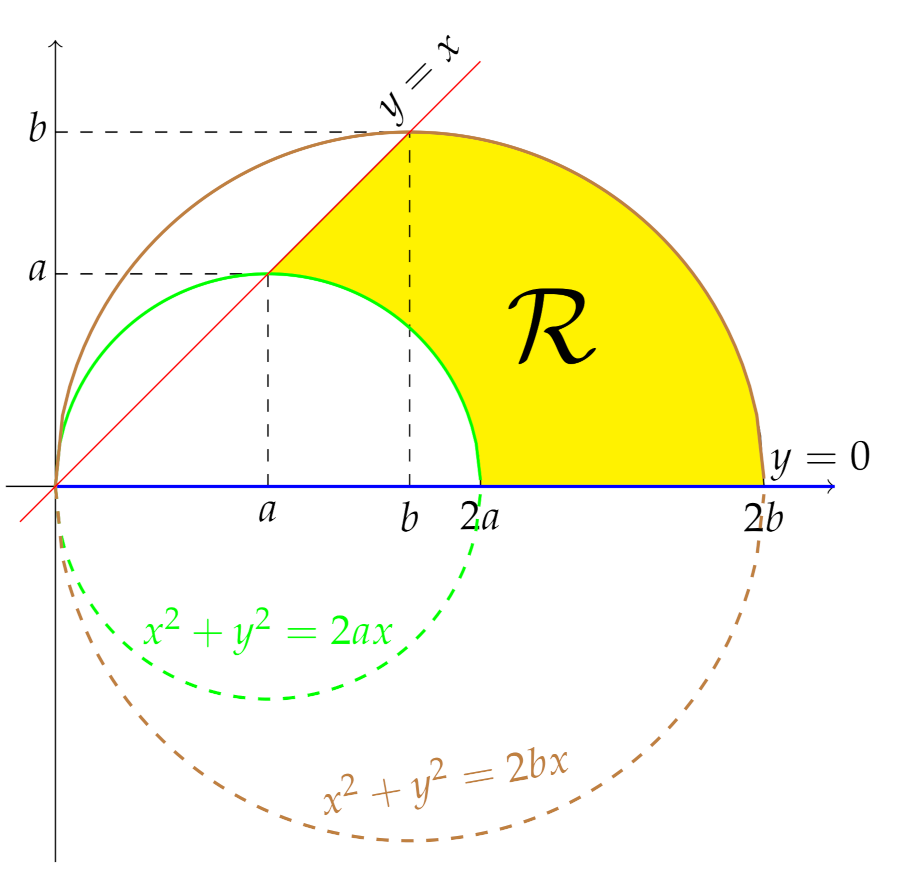
solves R ( x 2 + y 2 ) d x d y where R is the region bounded by x 2 + y 2 = 2 a x ; x 2 + y 2 = 2 b x ; y = x and y = 0 with 0 < a < b < 2 a (see Figure 2).
After running the above program, Derive returns:
Polar coordinates are useful when the expression x 2 + y 2 appears in the function to be integrated or in the region of integration.
A double integral in polar coordinates is computed by means of two definite integrals in a given order.
Previously, the change of variables to polar coordinates has to be done.
[Let us consider the polar coordinates change, x, = ρ cos ( θ ) and, y, = ρ sin ( θ ) .]
[The first step is the substitution of this variable change in function, x 2 + y 2 , and multiply this result by the Jacobian ρ .]
[In this case, the substitutions lead to integrate the function, ρ 3 ]
[Integrating the function, ρ 3 , with respect to variable, ρ , we get, ρ 4 4 ]
[Considering the limits of integration for this variable, we get, ( 4 b 4 4 a 4 ) cos ( θ ) 4 ]
[Finally, integrating this result with respect to variable, θ , the result is,
( b 4 a 4 ) sin ( θ ) cos ( θ ) 3 + 3 ( b 4 a 4 ) sin ( θ ) cos ( θ ) 2 3 θ ( a 4 b 4 ) 2 ]
Considering the limits of integration, the final result is:
b 4 a 4 ( 3 π + 8 ) 8
As for the previous program, DoublePolar also provides a warning message in case the result is suspected of being wrong because of a bad order in the limits of integration. Similar situations are considered in all programs in SMIS and will not be further commented on again. The code of the above two programs has been included here as examples of the developed code. The rest of the programs will not be displayed in the following sections but there is an appendix at the end of the paper where the code of all programs is provided.

3.3. Triple Integral

In this section, we describe the syntax and provide some examples of use of the programs dealing with triple integrals. Specifically, SMIS deals with three different programs to work with Cartesian, cylindrical and spherical coordinates respectively. The code of these programs can be found in Appendix A.2.

3.3.1. Triple Integral in Cartesian Coordinates

Syntax: Triple(f,u,u1,u2,v,v1,v2,w,w1,w2,myTheory,myStepwise)
Description: Compute, using Cartesian coordinates, the triple integral
D f ( u , v , w ) d u d v d w = w 1 w 2 v 1 v 2 u 1 u 2 f ( u , v , w ) d u d v d w , where D R 3 is the region: u 1 u u 2 ; v 1 v v 2 ; w 1 w w 2 .
Example 3.
Triple(xyz,z,0,sqrt(1-x 2 -y 2 ),y,0,sqrt(1-x 2 ),x,0,1,true,true)
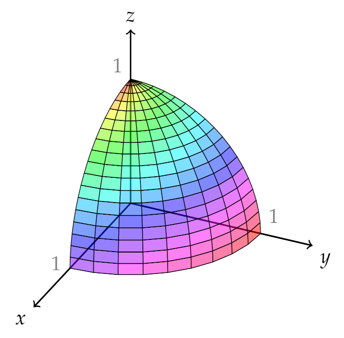
solves D x y z d x d y d z where D is the portion of sphere x 2 + y 2 + z 2 1 in the first octant x , y , z 0 (see Figure 3).
The result obtained in Derive is:
A triple integral is computed by means of three definite integrals in a given order.
[In this case, integrating the function, x y z , with respect to variable, z, we get, x y z 2 2 ]
[Considering the limits of integration for this variable, we get, x y ( x 2 + y 2 1 ) 2 ]
[Integrating the function, x y ( x 2 + y 2 1 ) 2 , with respect to variable, y, we get,
x y 2 ( 2 x 2 + y 2 2 ) 8 ]
[Considering the limits of integration for this variable, we get, x ( x 2 1 ) 2 8 ]
[Finally, integrating this result with respect to variable, x, the result is, ( x 2 1 ) 3 48 ]
Considering the limits of integration, the final result is
1 48

3.3.2. Triple Integral in Cylindrical Coordinates

Syntax: TripeCylindrical(f,u,u1,u2,v,v1,v2,w,w1,w2,myTheory,myStepwise,
myx,myy,myz)
Description: Compute, using cylindrical coordinates, the triple integral
D f ( x , y , z ) d x d y d z = w 1 w 2 v 1 v 2 u 1 u 2 ρ f ( ρ cos θ , ρ sin θ , z ) d u d v d w ,    where D R 3 is the region: u 1 u u 2 ; v 1 v v 2 ; w 1 w w 2 , in cylindrical coordinates ( u , v and w are z , ρ and θ in the right order of integration).
Note that the use of myx, myy and myz (set to x , y and z by default) allows the user to choose the role of which variables are considered as x, y or z. This way, the cylindrical variable change is:
myx = ρ cos ( θ ) myy = ρ sin ( θ ) myz = myz J a c o b i a n = ρ .
For example, if the user wants to make the cylindrical variable change as follows:
z = ρ cos ( θ ) ; x = ρ sin ( θ ) ; y = y ,
the values should be myx = z ; myy = x and myz = y . Therefore, the last three parameters of the program TripleCylindrical should be z , x and y .
Example 4.
TripleCylindrical(xyz,z,0,sqrt(1-rho 2 ),rho,0,1,theta,0,pi/2,true,true)
solves again the triple integral of Example 3 D x y z d x d y d z where D is the portion of sphere x 2 + y 2 + z 2 1 in the first octant x , y , z 0 but, in this case, using cylindrical coordinates (see Figure 3).
The result obtained in Derive is:
Cylindrical coordinates are useful when the expression x 2 + y 2 appears in the function to be integrated or in the region of integration and limits of z are easy to establish.
A triple integral in cylindrical coordinates is computed by means of three definite integrals in a given order.
Previously, the change of variables to cylindrical coordinates has to be done.
[Let us consider the cylindrical coordinates change, x, = ρ cos ( θ ) , y, = ρ sin ( θ ) , z,=, z]
[The first step is the substitution of this variable change in function, x y z , and multiply this result by the Jacobian ρ .]
[In this case, the substitutions lead to integrate the function, ρ 3 z sin ( θ ) cos ( θ ) ]
[Integrating the function, ρ 3 z sin ( θ ) cos ( θ ) , with respect to variable, z, we get,
ρ 3 z 2 sin ( θ ) cos ( θ ) 2 ]
[Considering the limits of integration for this variable, we get, ρ 3 ( 1 ρ 2 ) sin ( θ ) cos ( θ ) 2 ]
[Integrating the function, ρ 3 ( 1 ρ 2 ) sin ( θ ) cos ( θ ) 2 , with respect to variable, ρ , we get,
ρ 4 4 ρ 6 12 sin ( θ ) cos ( θ ) ]
[Considering the limits of integration for this variable, we get, sin ( θ ) cos ( θ ) 24 ]
[Finally, integrating this result with respect to variable, θ , the result is, sin ( θ ) 2 48 ]
Considering the limits of integration, the final result is
1 48

3.3.3. Triple Integral in Spherical Coordinates

Syntax: TripeSpherical(f,u,u1,u2,v,v1,v2,w,w1,w2,myTheory,myStepwise,myx,myy,myz)
Description: Compute, using spherical coordinates, the triple integral
D f ( x , y , z ) d x d y d z = w 1 w 2 v 1 v 2 u 1 u 2 ρ 2 cos ϕ f ( ρ cos ϕ cos θ , ρ cos ϕ sin θ , ρ sin ϕ ) d u d v d w ,
where D R 3 is the region: u 1 u u 2 ; v 1 v v 2 ; w 1 w w 2 , in spherical coordinates ( u , v and w are ρ , θ and ϕ in the right order of integration).
Note that the use of myx, myy and myz (set to x , y and z by default) allows the user to choose the role of which variables are considered as x, y or z. This way, the spherical variable change is:
myx = ρ cos ( ϕ ) cos ( θ ) myy = ρ cos ( ϕ ) sin ( θ ) myz = ρ sin ( ϕ ) J a c o b i a n = ρ 2 cos ( ϕ ) .
For example, if the user wants to make the spherical variable change as follows:
z = ρ cos ( ϕ ) cos ( θ ) ; x = ρ cos ( ϕ ) sin ( θ ) ; y = ρ sin ( ϕ ) ,
the values should be myx = z ; myy = x and myz = y . Therefore, the last three parameters of the program TripleSpherical should be z , x and y .
Example 5.
TripleSpherical(xyz,rho,0,1,theta,0,pi/2,phi,0,pi/2,true,true)
solves once again the triple integral of Example 3 D x y z d x d y d z where D is the portion of sphere x 2 + y 2 + z 2 1 in the first octant x , y , z 0 but, in this case, using spherical coordinates (see Figure 3).
The result obtained in Derive is:
Spherical coordinates are useful when the expression x 2 + y 2 + z 2 appears in the function to be integrated or in the region of integration.
A triple integral in spherical coordinates is computed by means of three definite integrals in a given order.
Previously, the change of variables to spherical coordinates has to be done.
[Let us consider the spherical coordinates change,
x, = ρ cos ( ϕ ) cos ( θ ) , y, = ρ cos ( ϕ ) sin ( θ ) , z, = ρ sin ( ϕ ) . ]
[The first step is the substitution of this variable change in function, x y z , and multiply this result by the Jacobian ρ 2 cos ( ϕ ) .]
[In this case, the substitutions lead to integrate the function,
ρ 5 sin ( θ ) cos ( θ ) sin ( ϕ ) cos ( ϕ ) 3 ]
[Integrating the function, ρ 5 sin ( θ ) cos ( θ ) sin ( ϕ ) cos ( ϕ ) 3 , with respect to variable, ρ , we get, ρ 6 sin ( θ ) cos ( θ ) sin ( ϕ ) . cos ( ϕ ) 3 6 ]
[Considering the limits of integration for this variable, we get:
sin ( θ ) cos ( θ ) sin ( ϕ ) cos ( ϕ ) 3 6 ]
[Integrating the function, sin ( θ ) cos ( θ ) sin ( ϕ ) cos ( ϕ ) 3 6 , with respect to variable, θ , we get, sin ( θ ) 2 sin ( ϕ ) cos ( ϕ ) 3 12 ].
[Considering the limits of integration for this variable, we get, sin ( ϕ ) cos ( ϕ ) 3 12 ].
[Finally, integrating this result with respect to variable, ϕ , the result is, cos ( ϕ ) 4 48 ].
Considering the limits of integration, the final result is:
1 48

3.4. Area of a Region R R 2

The area of a region R R 2 can be computed by the following double integral:
A r e a ( R ) = R 1 d x d y .
Therefore, depending on the use of Cartesian or polar coordinates, two different programs have been considered in SMIS. The code of these programs can be found in Appendix A.3.
Syntax:
  • Area(u,u1,u2,v,v1,v2,myTheory,myStepwise)
  • AreaPolar(u,u1,u2,v,v1,v2,myTheory,myStepwise,myx,myy)
Description: Compute, using Cartesian and polar coordinates respectively, the area of the region R R 2 determined by u 1 u u 2 ; v 1 v v 2 .
Example 6.
Area(y,x 2 ,sqrt(x),x,0,1,true,true)   computes the area of the region: x 2 y x ; 0 x 1 (see Figure 1).
The result obtained in Derive after the execution of the above program is:
The area of a region R can be computed by means of the double integral of function 1 over the region R.
To get a stepwise solution, run the program Double with function 1.
The area is:
1 3
Note that this program calls the program Double to obtain the final result. In the code, this program with the theory and stepwise options is set to false. The text "To get a stepwise solution, run the program Double with function 1" is displayed. This has been done in order not to display a detailed solution for this auxiliary computation and not to have a large text displayed. In any case, since the code is provided in the final appendix, the teacher can easily adapt this call to the specific needs. That is, if the teacher wants to show all the intermediate steps and theory depending on the user’s decision, the call to the Double function should be changed with the theory and stepwise parameters set to myTheory and myStepwise, respectively. In the following programs in the next sections, a similar situation occurs.
Example 7.
AreaPolar( ρ , 2 a cos θ , 2 b cos θ , θ ,0, π / 4 ,true,true)computes the area of the region bounded by x 2 + y 2 = 2 a x ; x 2 + y 2 = 2 b x ; y = x and y = 0 with 0 < a < b < 2 a (see Figure 2).
The result obtained in Derive after the execution of the above program is:
The area of a region R can be computed by means of the double integral of function 1 over the region R.
To get a stepwise solution, run the program DoublePolar with function 1.
The area is:
( π + 2 ) ( b 2 a 2 ) 4

3.5. Volume of a Solid D R 3

The volume of a solid D R 3 can be compute by the following triple integral:
V o l u m e ( D ) = D 1 d x d y d z .
Therefore, depending on the use of Cartesian, cylindrical or spherical coordinates, three different programs have been considered in SMIS. The code of these programs can be found in Appendix A.4.
Syntax:
  • Volume(u,u1,u2,v,v1,v2,w,w1,w2,myTheory,myStepwise)
  • VolumeCylindrical(u,u1,u2,v,v1,v2,w,w1,w2,myTheory,myStepwise,
                myx,myy,myz)
  • VolumeSpherical(u,u1,u2,v,v1,v2,w,w1,w2,myTheory,myStepwise,
                myx,myy,myz)
Description: Compute, using Cartesian, cylindrical and spherical coordinates respectively, the volume of the solid D R 3 determined by u 1 u u 2 ; v 1 v v 2 ; w 1 w w 2 .
Example 8.
Volume(z,0,sqrt(1-x 2 -y 2 ),y,0,sqrt(1-x 2 ),x,0,1,true,true)
computes the volume of the portion of sphere x 2 + y 2 + z 2 1 in the first octant x , y , z 0 (see Figure 3).
The result obtained in Derive after the execution of the above program is:
Derive CANNOT COMPUTE THIS INTEGRAL IN CARTESIAN COORDINATES.
In this example, Derive cannot perform the computation using Cartesian coordinates. This is a good example to make the student see the necessity and utility of a variable change. In this case, both cylindrical and spherical coordinates can be used as follows:
VolumeCylindrical(z,0,sqrt(1- ρ 2 ), ρ ,0,1, θ ,0, π / 2 ,true,true) computes the same volume using cylindrical coordinates.
The result obtained in Derive after the execution of the above program is:
The volume of a solid D can be computed by means of the triple integral of function 1 over the solid D.
To get a stepwise solution, run the program TripleCylindrical with function 1.
The volume is:
π 6
This example can also be solved using spherical coordinates with the following program: VolumeSpherical( ρ ,0,1, θ ,0, π / 2 , ϕ ,0, π / 2 ,true,true).

3.6. Surface Integrals

The surface integral of a scalar field f over a parametrized surface S w = w ( u , v ) ( u , v ) R u v R 2 is given by the double integral:
S f d S = R u v f ( u , v , w ( u , v ) ) 1 + w u 2 + w v 2 d u d v .
Therefore, depending on the use of Cartesian or polar coordinates, two different programs have been considered in SMIS. If the equation of the surface is given by w = w ( u , v ) , the variable on the left hand side and the value on the right hand side of this equation will be introduced separately in the second and the third parameter, respectively, of both programs. The code of these programs can be found in Appendix A.5.
Syntax:
  • SurfaceIntegral(f,myw,w,u,u1,u2,v,v1,v2,myTheory,myStepwise)
  • SurfaceIntegralPolar(f,myw,w,u,u1,u2,v,v1,v2,myTheory,myStepwise)
Description: Compute, using Cartesian and polar coordinates, respectively, the surface integral of a scalar field f over the surface S m y w = w ( u , v ) ( u , v ) R u v R 2 where R u v R 2 is determined by u 1 u u 2 ; v 1 v v 2 .
Example 9.
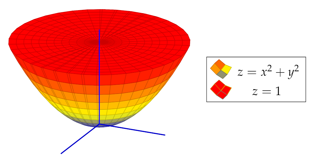
SurfaceIntegral( 1 + 4 x 2 + 4 y 2 ,z, x 2 + y 2 ,y, 1 x 2 , 1 x 2 ,x,-1,1,true,true)computes the surface integral S 1 + 4 x 2 + 4 y 2 d S over the portion of the paraboloid S z = x 2 + y 2 between z = 0 and z = 1 , using Cartesian coordinates (see Figure 4).
The result obtained in Derive after the execution of the above program is:
The surface integral of f over the surface S of equation w=w(u,v) can be computed by means of the double integral of f ( u , v , w ( u , v ) ) · 1 + ( w u ) 2 + ( w v ) 2 .
[In this case, f ( u , v , w ( u , v ) ) · 1 + ( w u ) 2 + ( w v ) 2 = , 4 x 2 + 4 y 2 + 1 ,
To get a stepwise solution, run the program Double with function, 4 x 2 + 4 y 2 + 1 ].
The surface integral is:
3 π
The same integral can also be solved using polar coordinates with the program SurfaceIntegralPolar( 1 + 4 x 2 + 4 y 2 ,z, x 2 + y 2 , ρ ,0,1, θ ,0, 2 π ,true,true).

3.7. Area of a Surface

The surface area of a parametrized surface S R 3 can be computed by the following surface integral:
A r e a ( S ) = S 1 d S .
Therefore, depending on the use of Cartesian or polar coordinates, two different programs have been considered in SMIS. The code of these programs can be found in Appendix A.6.
Syntax:
  • SurfaceArea(myw,w,u,u1,u2,v,v1,v2,myTheory,myStepwise)
  • SurfaceAreaPolar(myw,w,u,u1,u2,v,v1,v2,myTheory,myStepwise)
Description: Compute, using Cartesian and polar coordinates respectively, the area of the parametrized surface S m y w = w ( u , v ) ( u , v ) R u v R 2 where R u v R 2 is determined by u 1 u u 2 ; v 1 v v 2 .
Example 10.
SurfaceArea(z, x 2 + y 2 ,y, 1 x 2 , 1 x 2 ,x,-1,1,true,true)computes the area of the portion of the paraboloid S z = x 2 + y 2 between z = 0 and z = 1 , using Cartesian coordinates (see Figure 4).
The result obtained in Derive after the execution of the above program is:
The area of a surface S of equation w=w(u,v) can be computed by means of the surface integral of function 1.
To get a stepwise solution, run the program SurfaceIntegral with function 1.
The area of the surface is:
Derive CANNOT COMPUTE THIS INTEGRAL IN CARTESIAN COORDINATES.
Again, this is a great opportunity to point out the necessity of a variable change. With    SurfaceAreaPolar(z, x 2 + y 2 , ρ ,0,1, θ ,0, 2 π ,true,true),    this problem can be easily solved using polar coordinates.
The result obtained in Derive after the execution of the above program is:
The area of a surface S of equation w=w(u,v) can be computed by means of the surface integral of function 1.
To get a stepwise solution, run the program SurfaceIntegralPolar with function 1.
The area of the surface is:
π 5 5 6 1 6

3.8. Flux

The flux ϕ of a vector field F = ( P , Q , R ) over the parametrized surface S w = w ( u , v ) ( u , v ) R u v R 2 is given by the surface integral S F · n d S , where n is the unitary normal vector field associated with the orientation of S . Let us consider the gradient N = ( w w ( u , v ) ) = ( w u , w v , 1 ) , which is a normal vector field associated with S . Therefore, the unitary vector n coincides with either 1 | | N | | N or its opposite 1 | | N | | N , each of them corresponding to one of the two “sides" or orientations of S . Since | | N | | = 1 + ( w u ) 2 + ( w v ) 2 , in order to compute a flux, a surface integral or a double integral can be used as follows:
ϕ = S F · n d S = ± S F · N 1 | | N | | d S = ( 3 ) ± R u v F · N 1 | | N | | 1 + ( w u ) 2 + ( w v ) 2 d u d v = ± R u v F · N d u d v ,
where (3) is a link to the equation used to compute a surface integral (shown in Section 3.6). Therefore, the flux of F can be computed using the program SurfaceIntegral applied to function F · n or using the program Double applied to function F · N . The result will have a double sign ± providing this way the two possible values, from which we must select the one that corresponds to the orientation of S . When S is a closed surface, its positive orientation corresponds to the + sign of the outward normal vector, and its negative orientation corresponds to the sign of the inward normal vector.
Two different programs have been considered in SMIS to compute a flux depending on the use of Cartesian or polar coordinates. If the equation of the surface is given by w = w ( u , v ) , the variable on the left hand side and the value on the right hand side of this equation will be introduced separately in the second and the third parameter, respectively, of both programs. The code of these programs can be found in Appendix A.7. We decided to use the program Double since it does not require computation of | | N | | .
Syntax:
  • Flux(F,myw,w,u,u1,u2,v,v1,v2,myTheory,myStepwise)
  • FluxPolar(F,myw,w,u,u1,u2,v,v1,v2,myTheory,myStepwise)
Description: Compute, using Cartesian and polar coordinates respectively, the flux of a vector field F over an oriented surface S m y w = w ( u , v ) ( u , v ) R u v R 2 where R u v R 2 is determined by u 1 u u 2 ; v 1 v v 2 .
Example 11.
Flux( [ x , y , z ] ,z, x 2 + y 2 ,y, 1 x 2 , 1 x 2 ,x,-1,1,true,true)andFlux( [ x , y , z ] ,z,1,y, 1 x 2 , 1 x 2 ,x,-1,1,true,true)computes the flux of the vector field F = [ x , y , z ] over the closed and oriented surface bounded by the paraboloid S z = x 2 + y 2 and z = 1 , using Cartesian coordinates (see Figure 4).
The results obtained in Derive after the execution of the above two programs are:
The flux of F over the oriented surface S can be computed by means of the surface integral of F(u,v,w(u,v))·n(u,v), where n(u,v) is one of the two unitary normal vector fields associated with S. The flux can also be computed by means of the double integral of F(u,v,w(u,v))·N(u,v) where N(u,v) is the gradient.
[In this case, F(u,v,w(u,v))·N(u,v) =, x 2 y 2
To get a stepwise solution, run the program Double with function, x 2 y 2 ].
Depending on the use of the outward or inward normal vectors, the two different possible solutions of this flux are:
± π 2
The flux of F over the oriented surface S can be computed by means of the surface integral of F(u,v,w(u,v))·n(u,v) where n(u,v) is one of the two unitary normal vector fields associated with S. The flux can also be computed by means of the double integral of F(u,v,w(u,v))·N(u,v) where N(u,v) is the gradient.
[In this case, F(u,v,w(u,v))·N(u,v) =,1
To get a stepwise solution, run the program Double with function, 1].
Depending on the use of the outward or inward normal vectors, the two different possible solutions of this flux are:
± π
Note that the total flux is the sum of the flux over the paraboloid and the flux over the plane z = 1 . If we consider the outward normal vector of the closed surface, the results are, respectively, π 2 and π . Thus, the total flux is 3 π 2 .
FluxPolar( [ x , y , z ] ,z, x 2 + y 2 , ρ ,0,1, θ ,0, 2 π ,true,true)     and
FluxPolar( [ x , y , z ] ,z,1, ρ ,0,1, θ ,0, 2 π ,true,true)    can be used to solve the same example using polar coordinates.

3.9. Divergence Theorem

The divergence theorem (also known as Gauss’s theorem) allows computation of the flux over a closed surface by means of a triple integral as follows:
Theorem 1
(Divergence). Let F ( x , y , z ) = P ( x , y , z ) , Q ( x , y , z ) , R ( x , y , z ) be a continuous vector field defined over a solid D R 3 bounded by the closed surface S . Let n be the outward unit normal vector field associated with S . Let div F = P x + Q y + R z , the divergence of F . Then, ϕ , the flux of F along S is:
ϕ = S F · n d S = D div F d x d y d z .
Therefore, depending on the use of Cartesian, cylindrical or spherical coordinates, three different programs have been considered in SMIS. The code of these programs can be found in Appendix A.8.
Syntax:
  • FluxDivergence(F,u,u1,u2,v,v1,v2,w,w1,w2,myTheory,myStepwise)
  • FluxDivergenceCylindrical(F,u,u1,u2,v,v1,v2,w,w1,w2,myTheory,
                myStepwise)
  • FluxDivergenceSpherical(F,u,u1,u2,v,v1,v2,w,w1,w2,myTheory,
                myStepwise)
Description: Compute, using the divergence theorem, the flux of the vector field F over the closed surface S that encloses the solid D R 3 determined by u 1 u u 2 ; v 1 v v 2 ; w 1 w w 2 , using Cartesian, cylindrical and spherical coordinates respectively.
Example 12.
FluxDivergence([x,y,z],z,x 2 +y 2 ,1,y,-sqrt(1-x 2 ),sqrt(1-x 2 ),x,-1,1,true,true)   computes the flux of the vector field F = [ x , y , z ] over the closed surface bounded by the paraboloid S z = x 2 + y 2 and z = 1 , using Cartesian coordinates (see Figure 4).
The result obtained in Derive after the execution of the above program is:
The flux of F over the closed surface S that encloses the solid D can be computed by means of the triple integral of the divergence of F over the solid D.
[In this case, the divergence of F is, 3, To get a stepwise solution, run the program Triple with function", 3].
The flux is:
3 π 2
FluxDivergenceCylindrical([x,y,z],z, ρ 2 ,1, ρ ,0,1, θ ,0, 2 π ,true,true) also computes the previous flux using cylindrical coordinates.
Example 13.
FluxDivergenceSpherical([x,y,z], ρ ,0,a, θ ,0, 2 π , ϕ , π / 2 , π / 2 ,true,true)computes the flux of the vector field F = [ x , y , z ] over the closed sphere S x 2 + y 2 + z 2 = a 2 using spherical coordinates.
The result obtained in Derive after the execution of the above program is:
The flux of F over the closed surface S that encloses the solid D can be computed by means of the triple integral of the divergence of F over the solid D.
[In this case, the divergence of F is, 3, To get a stepwise solution, run the program TripleSpherical with function, 3].
The flux is:
4 π a 3

3.10. Green’s Theorem

Green’s theorem relates the calculation of a line integral over a closed path with a double integral over the region of R 2 that the path encloses as follows:
Theorem 2
(Green). Let C be a positive oriented simple closed path in R 2 and R R 2 the region it encloses. Let P ( x , y ) and Q ( x , y ) be two scalar fields defined on R with continuous partial derivatives. Then:
C P ( x , y ) d x + Q ( x , y ) d y = R Q ( x , y ) x P ( x , y ) y d x d y .
Therefore, depending on the use of Cartesian or polar coordinates, two different programs have been considered in SMIS. The code of these programs can be found in Appendix A.9.
Syntax:
  • Green(P,Q,u,u1,u2,v,v1,v2,myTheory,myStepwise)
  • GreenPolar(P,Q,u,u1,u2,v,v1,v2,myTheory,myStepwise)
Description: Compute C P ( x , y ) d x + Q ( x , y ) d y using a double integral over the region R R 2 bounded by C with limits u 1 u u 2 ; v 1 v v 2 , using Cartesian and polar coordinates respectively.
Example 14.
Green( y 3 , x 4 + x 2 ,y,0,1,x,0,1,true,true)computes the line integral C y 3 d x + ( x 4 + x 2 ) d y along the segments joining the points (0,0), (1,0), (1,1), (0,1) and back to (0,0).
The result obtained in Derive after the execution of the above program is:
The line integral of Pdx+Qdy over the closed path C that encloses the region R, can be computed by the double integral of the expression DIF(Q,x)-DIF(P,y) over R.
[In this case, DIF(Q,x)-DIF(P,y) =, 4 x 3 + 2 x 3 y 2 , To get a stepwise solution, run the program Double with function, 4 x 3 + 2 x 3 y 2 ]
The line integral is:
1
Example 15.
GreenPolar( y 3 , x 4 + x 2 , ρ ,0,a, θ ,0, 2 π ,true,true)computes the line integral C y 3 d x + ( x 4 + x 2 ) d y along the circumference x 2 + y 2 = a 2 .
The result obtained in Derive after the execution of the above program is:
The line integral of Pdx+Qdy over the closed path C that encloses the region R, can be computed by the double integral of the expression DIF(Q,x)-DIF(P,y) over R.
[In this case, DIF(Q,x)-DIF(P,y) =, 4 x 3 + 2 x 3 y 2 , To get a stepwise solution, run the program DoublePolar with function, 4 x 3 + 2 x 3 y 2 ]
The line integral is:
3 π a 4 4

4. The Use of SMIS in Mathematics Education

In this section, we want to point out the importance of SMIS for Mathematics Education. It is well-known that CAS can help the users to obtain the final result to different math problems but we think that the normal use given to CAS within Math Education has not reached the optimum approach. In most cases, CAS are considered and used as “black boxes” to which the user asks for a result and simply obtains it. We believe that CAS must be used in Math Education as “white boxes”. That is, CAS should return not only the final result but also all the major steps needed to get to it. For example, if a student solves an integral and later checks with a CAS to see if the result is right or not, what happens if the result does not match with the one the student obtained? Or what happens if the result is equivalent but the student does not recognize it? [25]. It would be more useful to see the whole process of resolution and not only the final result. This way, firstly, the student may detect the step(s) in which an error occurs or, secondly, if the student does not know how to proceed in an intermediate step, he can check the stepwise solution and find out how to proceed.
Nowadays, it is true that there are some CAS or web applications that provide intermediate steps but not for all topics and not always without a subscription which could require a large amount of money. Furthermore, in advanced topics such as the ones dealt with in SMIS, these stepwise alternatives are very few. On the other hand, an already made application could not provide the stepwise solution in the same way that the student learned. With SMIS, the teacher can introduce the theory and intermediate steps that follow the approach given at lectures. We have developed “our version” of SMIS but the teacher can easily adapt this version to specific needs. This way, SMIS is not only a stepwise solver but is also a template of how a CAS can be used to help in the teaching and learning process.
Furthermore, since we have developed programs to deal with multiple integration using different orders of integration or different coordinate systems, the teacher can use these facilities to help the student learn the importance of the appropriate order of integration and the best coordinate system in a specific exercise. This fact is of special interest when the CAS cannot compute the integrals in a specific order or in a coordinate system.
Regarding the use we have made of previous Spanish versions of SMIS or other stepwise solvers for other topics aimed to Engineering degrees, different studies have been developed with students which reveal that using this way of working with CAS improves their understanding of the topics dealt. For example, three PhD theses developed by some of the authors of this paper revealed that when working with stepwise solvers their marks in exams were up to more than 25% higher than when without working with these tools [8,26,27].
In addition, due to the COVID pandemic [28], which led in many cases to a teaching process without in situ lectures, extra materials and procedures (pdf files, videos, online lectures, …) had to be developed [29,30]. In this environment, the use of stepwise solvers has been very well valued by our students. Specifically, several questions were asked of the students, obtaining more than 4.5 points out of 5 in all of them. That is, greater that 90% of the top marks.
Another important fact is the development of appropriate tasks for students when working in computer lectures. In the last 15 years, one of the objectives of our computer lectures is to foster critical thinking in students. The result obtained with a CAS is not always correct  [31]. The use of programming with a CAS also allows the control of these possible errors. Furthermore, when the students develop a program for solving a specific kind of exercise, it will be easier for them to solve this kind of exercise by hand later, since they need to acquire a good background in order to be able to develop the program. That is why, in the task we develop with our students in the computer lectures, they not only have to apply programs already built by the teachers but also some exercises require them to develop programs themselves.

5. Conclusions and Future Work

In this paper we have introduced SMIS, a new stepwise solver for Multiple Integration. Although the programs have been developed in the CAS Derive, since the code of all programs is available in the paper, it can be easily migrated to any other computer algebra system. We have developed the following two different files:
  • SMIS.mth is a library in Derive containing all the programs of SMIS. With this library, we achieve one of the main objectives in this paper: to increase the capabilities of a CAS. When loading this library in Derive, the user can use its programs to deal directly with double, triple and surface integrals and their applications. As mentioned before, it is easy to migrate this library to other CAS so that their capabilities would also be increased.
  • SMIS.dfw is a tutorial in Derive which provides detailed examples of the uses of all the programs of SMIS. In addition, since the developed programs can optionally provide stepwise results, with this fact we achieve another important objective of this paper: SMIS can be used as a tutorial for the teaching and learning process of multiple integration and its applications which can be very useful in mathematics subjects dealing with multiple integration in Math, Physics and Engineering degrees. Again, this tutorial can be easily migrated to other CAS and, therefore, this tutorial can be used in other CAS. In addition, we have proposed “our version” of stepwise solutions but the provided code of all programs can also be adapted to the specific needs of the teacher.
We have also considered two global variables, Theory and Stepwise, initially set by default to true, which control whether the theory involved and intermediate steps are displayed or not. Again, the deepness in both theory and stepwise solutions can be easily adapted to the specific needs of the user. When setting any of these global variables to false, the results provided by the programs are simplified. In addition, the user can execute any program in the SMIS settings to true or false, two optional parameters which allow us to display or not the theory and/or stepwise solution independently of the values of the global variables.
We can conclude that adapting SMIS to specific needs is an easy task and will provide an important tool for both objectives: the increment of capabilities of a CAS and as an aid in the teaching and learning processes in the topic “Multiple integration”.
SMIS can be freely downloaded at https://acortar.link/SMIS (accessed on 22 September 2021).

Future Work

As related future works we can point out three different lines:
  • The migration of SMIS and other previously developed solvers for Partial Differential Equations [7], Line integrals [32] or Automated Theorem Provers [33] from Derive to a more portable environment such as Python [2] using SymPy [19];
  • The development of new stepwise solvers in Python for other mathematical topics;
  • The integration of all solvers in a free web online application, which can be used in different languages.
Regarding the first and the third lines, we have already developed a first approach. We have migrated some programs to Python to solve different types of Differential Equations following the same idea of optional theory and stepwise information. This draft version runs in a local web browser and the user can choose between English, Spanish or French. Our priority will be to develop a full version of a specific topic and make it freely accessible in an online application. In parallel, we want to go further with the second line mentioned before developing new stepwise solvers for other topics such as Complex Analysis, Elementary Calculus, Algebra, and so forth.
In the long term, the final goal will be the development of a free online web application to deal with a great variety of mathematical topics with optional stepwise and theory information and in different languages.

Author Contributions

All authors contributed equally to this work. In addition, J.L.G.-G. wrote the first draft of the paper. All authors have read and agreed to the published version of the manuscript.

Funding

This research received no external funding.

Institutional Review Board Statement

Not applicable.

Informed Consent Statement

Not applicable.

Acknowledgments

We thank the anonymous reviewers for their suggestions and comments which have improved the quality of the paper.

Conflicts of Interest

The authors declare no conflict of interest.

Abbreviations

   The following abbreviations are used in this manuscript:
CASComputer Algebra System
SMISStepwise Multiple Integration Solver
SFOPDESStepwise First Order Partial Differential Equations Solver

Appendix A. Code of Programs

The file SMIS.mth contents the code of all programs of SMIS. It can be downloaded at https://acortar.link/SMIS (accessed on 22 September 2021).
In any case, in this appendix we include the code of all programs of SMIS. This way, the readers who cannot use Derive, can see the code and even adapt it to the desired CAS.

Appendix A.1. Double Integral

Double(f,u,u1,u2,v,v1,v2,myTheory:=Theory,myStepwise:=Stepwise,I_):=
Prog(
   If(myTheory,
      DISPLAY("A double integral is computed by means of two definite
         integrals in a given order.") ),
   I_:=INT(f,u,u1,u2),
   If (myStepwise,
      Prog(
         DISPLAY(["In this case, integrating  the function", f, "with
            respect to variable", u, "we get", INT(f,u)]),
         DISPLAY(["Considering the limits of integration for this
            variable, we get",I_]),
         DISPLAY(["Finally, integrating this result with respect to
            variable", v, "the result is", INT(I_,v)]),
         DISPLAY("Considering the limits of integration, the~final
            result is") ) ),
   I_:=INT(I_,v,v1,v2),
   If((POSITION(u,VARIABLES(I_)) or POSITION(v,VARIABLES(I_)))/=false,
     RETURN [I_,"WARNING!: SUSPICIOUS RESULT. MAYBE THE INTEGRATION
                 ORDER IS WRONG"] ),
   RETURN I_
)
DoublePolar(f,u,u1,u2,v,v1,v2,myTheory:=Theory,myStepwise:=Stepwise,
   myx:=x,myy:=y,f_,I_):=
Prog(
   f_:= rho SUBST(f, [myx,myy], [rho cos(theta), rho sin(theta)]),
   If(myTheory,
      Prog(
         DISPLAY("Polar coordinates are useful when the expression
            x^2+y^2 appears in the function to be integrated or in the
            region of integration."),
         DISPLAY("A double integral in polar coordinates is computed
            by means of two definite integrals in a given order."),
         DISPLAY("Previously, the~change of variables to polar
            coordinates has to be done.") ) ),
   I_:=INT(f_,u,u1,u2),
   If (myStepwise,
      Prog(
         DISPLAY(["Let us consider the polar coordinates change",
            myx, "=rho cos(theta)",
            myy, "=rho sin(theta)"]),
         DISPLAY(["The first step is the substitution of this variable
            change in function", f, "and multiply this result by the
            Jacobian rho."]),
         DISPLAY(["In this case, the~result leads to integrate the
            function", f_]),
         DISPLAY(["Integrating  the function", f_, "with respect to
         variable", u, "we get", INT(f_,u)]),
         DISPLAY(["Considering the limits of integration for this
            variable, we get",I_]),
         DISPLAY(["Finally, integrating this result with respect to
            variable", v, "the result is", INT(I_,v)]),
         DISPLAY("Considering the limits of integration, the~final
            result is") ) ),
   I_:=INT(I_,v,v1,v2),
   If((POSITION(x,VARIABLES(I_)) or POSITION(y,VARIABLES(I_)) or
       POSITION(u,VARIABLES(I_)) or POSITION(v,VARIABLES(I_)))/=false,
     RETURN [I_,"WARNING!: SUSPICIOUS RESULT. MAYBE THE INTEGRATION
                 ORDER IS WRONG OR THE VARIABLES CHANGE HAS NOT BEEN
                 DONE IN THE LIMITS OF INTEGRATION"] ),
   RETURN I_
)

Appendix A.2. Triple Integral

Triple(f,u,u1,u2,v,v1,v2,w,w1,w2,
       myTheory:=Theory,myStepwise:=Stepwise,I1_,I2_):=
Prog(
   If(myTheory,
      DISPLAY("A triple integral is computed by means of three definite
         integrals in a given order.") ),
   I1_:=INT(f,u,u1,u2),
   I2_:=INT(I1_,v,v1,v2),
   If (myStepwise,
      Prog(
         DISPLAY(["In this case, integrating  the function", f, "with
            respect to variable", u, "we get", INT(f,u)]),
         DISPLAY(["Considering the limits of integration for this
            variable, we get",I1_]),
         DISPLAY(["Integrating  the function", I1_, "with
            respect to variable", v, "we get", INT(I_1,v)]),
         DISPLAY(["Considering the limits of integration for this
            variable, we get",I2_]),
         DISPLAY(["Finally, integrating this result with respect to
            variable", w, "the result is", INT(I2_,w)]),
         DISPLAY("Considering the limits of integration, the~final
            result is") ) ),
   I1_:=INT(I2_,w,w1,w2),
   If((POSITION(u,VARIABLES(I1_)) or POSITION(v,VARIABLES(I1_))
        or POSITION(w,VARIABLES(I1_)))/=false,
     RETURN [I1_,"WARNING!: SUSPICIOUS RESULT. MAYBE THE INTEGRATION
                 ORDER IS WRONG"] ),
   RETURN I1_
)
TripleCylindrical(f,u,u1,u2,v,v1,v2,w,w1,w2,myTheory:=Theory,
            myStepwise:=Stepwise,myx:=x,myy:=y,myz:=z,f_,I1_,I2_):=
Prog(
   f_:= rho SUBST(f,[myx,myy,myz],[rho cos(theta), rho sin(theta),myz]),
   If(myTheory,
      Prog(
         DISPLAY("Cylindrical coordinates are useful when the expression
            x^2+y^2 appears in the function to be integrated"),
         DISPLAY("or in the region of integration and limits of z are
            easy to establish."),
         DISPLAY("A triple integral in cylindrical coordinates is
            computed by means of three definite integrals in a given
            order."),
         DISPLAY("Previously, the~change of variables to cylindrical
            coordinates has to be done.") ) ),
   I1_:=INT(f_,u,u1,u2),
   I2_:=INT(I1_,v,v1,v2),
   If (myStepwise,
      Prog(
         DISPLAY(["Let us consider the cylindrical coordinates change",
            myx, "=rho cos(theta)",
            myy, "=rho sin(theta)",
            myz,"=",myz]),
         DISPLAY(["The first step is the substitution of this variable
            change in function", f, "and multiply this result by the
            Jacobian rho."]),
         DISPLAY(["In this case, the~substitutions lead to integrate
            the function", f_]),
         DISPLAY(["Integrating  the function", f_, "with respect to
         variable", u, "we get", INT(f_,u)]),
         DISPLAY(["Considering the limits of integration for this
            variable, we get",I1_]),
         DISPLAY(["Integrating  the function", I1_, "with
            respect to variable", v, "we get", INT(I1_,v)]),
         DISPLAY(["Considering the limits of integration for this
            variable, we get",I2_]),
         DISPLAY(["Finally, integrating this result with respect to
            variable", w, "the result is", INT(I2_,w)]),
         DISPLAY("Considering the limits of integration, the~final
            result is") ) ),
   I1_:=INT(I2_,w,w1,w2),
   If((POSITION(x,VARIABLES(I1_)) or POSITION(y,VARIABLES(I1_)) or
       POSITION(z,VARIABLES(I1_)) or POSITION(u,VARIABLES(I1_)) or
       POSITION(v,VARIABLES(I1_)) or POSITION(w,VARIABLES(I1_)))
          /=false,
     RETURN [I1_,"WARNING!: SUSPICIOUS RESULT. MAYBE THE INTEGRATION
                 ORDER IS WRONG OR THE VARIABLES CHANGE HAS NOT BEEN
                 DONE IN THE LIMITS OF INTEGRATION"] ),
   RETURN I1_
)
TripleSpherical(f,u,u1,u2,v,v1,v2,w,w1,w2,myTheory:=Theory,
                myStepwise:=Stepwise,myx:=x,myy:=y,myz:=z,f_,I1_,I2_):=
Prog(
   f_:= rho^2 cos(phi) SUBST(f, [myx,myy,myz],
      [rho cos(phi) cos(theta), rho cos(phi) sin(theta), rho sin(phi)]),
   If(myTheory,
      Prog(
         DISPLAY("Spherical coordinates are useful when the expression
            x^2+y^2+z^2 appears in the function to be integrated"),
         DISPLAY("or in the region of integration."),
         DISPLAY("A triple integral in spherical coordinates is computed
            by means of three definite integrals in a given order."),
         DISPLAY("Previously, the~change of variables to spherical
            coordinates has to be done.") ) ),
   I1_:=INT(f_,u,u1,u2),
   I2_:=INT(I1_,v,v1,v2),
   If (myStepwise,
      Prog(
         DISPLAY(["Let us consider the spherical coordinates change",
            myx, "=rho cos(phi) cos(theta)",
            myy, "=rho cos(phi) sin(theta)",
            myz, "=rho sin(phi)"]),
         DISPLAY(["The first step is the substitution of this
            variable change in function", f, "and multiply this
            result by the Jacobian rho^2 cos(phi)."]),
         DISPLAY(["In this case, the~substitutions lead to integrate
            the function", f_]),
         DISPLAY(["Integrating  the function", f_, "with respect to
         variable", u, "we get", INT(f_,u)]),
         DISPLAY(["Considering the limits of integration for this
            variable, we get",I1_]),
         DISPLAY(["Integrating  the function", I1_, "with
            respect to variable", v, "we get", INT(I1_,v)]),
         DISPLAY(["Considering the limits of integration for this
            variable, we get",I2_]),
         DISPLAY(["Finally, integrating this result with respect to
            variable", w, "the result is", INT(I2_,w)]),
         DISPLAY("Considering the limits of integration, the~final
            result is") ) ),
   I1_:=INT(I2_,w,w1,w2),
   If((POSITION(x,VARIABLES(I1_)) or POSITION(y,VARIABLES(I1_)) or
       POSITION(z,VARIABLES(I1_)) or POSITION(u,VARIABLES(I1_)) or
       POSITION(v,VARIABLES(I1_)) or POSITION(w,VARIABLES(I1_)))
          /=false,
     RETURN [I1_,"WARNING!: SUSPICIOUS RESULT. MAYBE THE INTEGRATION
                 ORDER IS WRONG OR THE VARIABLES CHANGE HAS NOT BEEN
                 DONE IN THE LIMITS OF INTEGRATION"] ),
   RETURN I1_
)

Appendix A.3. Area of a Region R R 2

Area(u,u1,u2,v,v1,v2,myTheory:=Theory,myStepwise:=Stepwise):=
Prog(
   If(myTheory,
      DISPLAY("The area of a region R can be computed by means of the
         double integral of function 1 over the region R.") ),
   If(myStepwise,
      DISPLAY("To get a stepwise solution, run the program Double
         with function 1.") ),
   If(myTheory or myStepwise,
      DISPLAY("The area is:") ),
   RETURN Double(1,u,u1,u2,v,v1,v2,false,false)
)
AreaPolar(u,u1,u2,v,v1,v2,myTheory:=Theory,myStepwise:=Stepwise,
          myx:=x,myy:=y):=
Prog(
   If(myTheory,
      DISPLAY("The area of a region R can be computed by means of the
         double integral of function 1 over the region R.") ),
   If(myStepwise,
      DISPLAY("To get a stepwise solution, run the program DoublePolar
         with function 1.") ),
   If(myTheory or myStepwise,
      DISPLAY("The area is:") ),
   RETURN DoublePolar(1,u,u1,u2,v,v1,v2,false,false,myx,myy)
)

Appendix A.4. Volume of a Solid D R 3

Volume(u,u1,u2,v,v1,v2,w,w1,w2,myTheory:=Theory,myStepwise:=Stepwise):=
Prog(
   If(myTheory,
      DISPLAY("The volume of a solid D can be computed by means of the
         triple integral of function 1 over the solid D.") ),
   If(myStepwise,
      DISPLAY("To get a stepwise solution, run the program Triple
         with function 1.") ),
   If(myTheory or myStepwise,
      DISPLAY("The volume is:") ),
   RETURN Triple(1,u,u1,u2,v,v1,v2,w,w1,w2,false,false)
)
VolumeCylindrical(u,u1,u2,v,v1,v2,w,w1,w2,myTheory:=Theory,
        myStepwise:=Stepwise,myx:=x,myy:=y,myz:=z):=
Prog(
   If(myTheory,
      DISPLAY("The volume of a solid D can be computed by means of the
         triple integral of function 1 over the solid D.") ),
   If(myStepwise,
      DISPLAY("To get a stepwise solution, run the program
         TripleCylindrical with function 1.") ),
   If(myTheory or myStepwise,
      DISPLAY("The volume is:") ),
   RETURN TripleCylindrical(1,u,u1,u2,v,v1,v2,w,w1,w2,false,false,
             myx,myy,myz)
)
VolumeSpherical(u,u1,u2,v,v1,v2,w,w1,w2,myTheory:=Theory,
        myStepwise:=Stepwise,myx:=x,myy:=y,myz:=z):=
Prog(
   If(myTheory,
      DISPLAY("The volume of a solid D can be computed by means of the
         triple integral of function 1 over the solid D.") ),
   If(myStepwise,
      DISPLAY("To get a stepwise solution, run the program
         TripleSpherical with function 1.") ),
   If(myTheory or myStepwise,
      DISPLAY("The volume is:") ),
   RETURN TripleSpherical(1,u,u1,u2,v,v1,v2,w,w1,w2,false,false,
             myx,myy,myz)
)

Appendix A.5. Surface Integrals

SurfaceIntegral(f,myw,w,u,u1,u2,v,v1,v2,myTheory:=Theory,
                myStepwise:=Stepwise,f_):=
Prog(
   f_:=subst(f,myw,w) sqrt(1+dif(w,u)^2+dif(w,v)^2),
   If(myTheory,
      DISPLAY("The surface integral of f over the surface
         S of equation w=w(u,v) can be computed by means of the
         double integral of f(u,v,w(u,v)) sqrt{1+(w’_u)^2+(w’_v)^2}.") ),
   If(myStepwise,
      DISPLAY(["In this case, f(u,v,w(u,v)) sqrt{1+(w’_u)^2+(w’_v)^2} =",
         f_, "To get a stepwise solution, run the program Double with
         function", f_]) ),
   If(myTheory or myStepwise,
      DISPLAY("The surface integral is:") ),
   RETURN Double(f_,u,u1,u2,v,v1,v2,false,false)
)
SurfaceIntegralPolar(f,myw,w,u,u1,u2,v,v1,v2,
            myTheory:=Theory,myStepwise:=Stepwise,myx_,myy_,f_):=
Prog(
   myx_ := FIRST({x,y,z}\{myw},
   myy_ := FIRST({x,y,z}\{myx_,myw}),
   f_:=subst(f,myw,w) sqrt(1+dif(w,myx_)^2+dif(w,myy_)^2),
   If(myTheory,
      DISPLAY("The surface integral of f over the surface
         S of equation w=w(u,v) can be computed by means of the double
         integral of f(u,v,w(u,v)) sqrt{1+(w’_u)^2+(w’_v)^2}.") ),
   If(myStepwise,
      DISPLAY(["In this case, f(u,v,w(u,v)) sqrt{1+(w’_u)^2+(w’_v)^2} =",
         f_, "To get a stepwise solution, run the program DoublePolar
         with function", f_]) ),
   If(myTheory or myStepwise,
      DISPLAY("The surface integral is:") ),
   RETURN DoublePolar(f_,u,u1,u2,v,v1,v2,false,false,myx_,myy_)
)

Appendix A.6. Area of a Surface

SurfaceArea(myw,w,u,u1,u2,v,v1,v2,myTheory:=Theory,
            myStepwise:=Stepwise) :=
Prog(
   If(myTheory,
      DISPLAY("The area of a surface S of equation w=w(u,v) can be
         computed by means of the surface integral of function 1.") ),
   If(myStepwise,
      DISPLAY("To get a stepwise solution, run the program
         SurfaceIntegral with function 1.") ),
   If(myTheory or myStepwise,
      DISPLAY("The area of the surface is:") ),
   RETURN SurfaceIntegral(1,myw,w,u,u1,u2,v,v1,v2,false,false)
)
SurfaceAreaPolar(myw,w,u,u1,u2,v,v1,v2,myTheory:=Theory,
                 myStepwise:=Stepwise) :=
Prog(
   If(myTheory,
      DISPLAY("The area of a surface S of equation w=w(u,v) can be
         computed by means of the surface integral of function 1.") ),
   If(myStepwise,
      DISPLAY("To get a stepwise solution, run the program
         SurfaceIntegralPolar with function 1.") ),
   If(myTheory or myStepwise,
   DISPLAY("The area of the surface is:") ),
   RETURN SurfaceIntegralPolar(1,myw,w,u,u1,u2,v,v1,v2,false,false)
)

Appendix A.7. Flux

Flux(F,myw,w,u,u1,u2,v,v1,v2,myTheory:=Theory,myStepwise:=Stepwise,f_):=
Prog(
   f_:=subst(F·grad(myw-w),myw,w),
   If(myTheory,
      Prog(
         DISPLAY("The flux of F over the oriented surface S can be
            computed by means of the surface integral of"),
         DISPLAY("F(u,v,w(u,v))·n(u,v) where n(u,v) is one of the two
            unitary normal vector fields associated with S."),
         DISPLAY("The flux can also be computed by means of
            the double integral of"),
         DISPLAY("F(u,v,w(u,v))·N(u,v) where N(u,v) is the gradient."))),
   If(myStepwise,
      DISPLAY(["In this case, F(u,v,w(u,v))·N(u,v) =",f_, "To get a
      stepwise solution, run the program Double with function", f_]) ),
   If(myTheory or myStepwise,
      DISPLAY("Depending on the use of the outward or inward normal
         vectors, the~two different possible solutions of this flux
         are:") ),
   RETURN ±Double(f_,u,u1,u2,v,v1,v2,false,false)
)
FluxPolar(F,myw,w,u,u1,u2,v,v1,v2,
            myTheory:=Theory,myStepwise:=Stepwise,myx_,myy_,f_):=
Prog(
   myx_ := FIRST({x,y,z}\{myw},
   myy_ := FIRST({x,y,z}\{myx_,myw}),
   f_:=subst(F·grad(myw-w),myw,w),
   If(myTheory,
      Prog(
         DISPLAY("The flux of F over the oriented surface S can be
            computed by means of the surface integral of"),
         DISPLAY("F(u,v,w(u,v))·n(u,v) where n(u,v) is one of the two
            unitary normal vector fields associated with S."),
         DISPLAY("The flux can also be computed by means of
            the double integral of"),
         DISPLAY("F(u,v,w(u,v))·N(u,v) where N(u,v) is the gradient."))),
   If(myStepwise,
      DISPLAY(["In this case, F(u,v,w(u,v))·N(u,v) =",f_,
         "To get a stepwise solution, run the program DoublePolar with
            function", f_]) ),
   If(myTheory or myStepwise,
      DISPLAY("Depending on the use of the outward or inward normal
         vectors, the~two different possible solutions of this flux
         are:") ),
   RETURN ±DoublePolar(f_,u,u1,u2,v,v1,v2,false,false,myx_,myy_)
)

Appendix A.8. Divergence Theorem

FluxDivergence(F,u,u1,u2,v,v1,v2,w,w1,w2,myTheory:=Theory,
               myStepwise:=Stepwise,f_):=
Prog(
   f_:=div(F),
   If(myTheory,
      DISPLAY("The flux of F over the closed surface S that
      encloses the solid D can be computed by means of the triple
      integral of the divergence of F over the solid D.") ),
   If(myStepwise,
      DISPLAY(["In this case, the~divergence of F is", f_, "To get a
         stepwise solution, run the program Triple with function",f_]) ),
   If(myTheory or myStepwise,
      DISPLAY("The flux is:") ),
   RETURN Triple(f_,u,u1,u2,v,v1,v2,w,w1,w2,false,false)
)
FluxDivergenceCylindrical(F,u,u1,u2,v,v1,v2,w,w1,w2,myTheory:=Theory,
            myStepwise:=Stepwise,myx:=x,myy:=y,myz:=z,f_):=
Prog(
   f_:=div(F),
   If(myTheory,
      DISPLAY("The flux of F over the closed surface S that
         encloses the solid D can be computed by means of the triple
         integral of the divergence of F over the solid D.") ),
   If(myStepwise,
      DISPLAY(["In this case, the~divergence of F is", f_, "To get a
         stepwise solution, run the program TripleCylindrical with
         function",f_]) ),
   If(myTheory or myStepwise,
      DISPLAY("The flux is:") ),
   RETURN TripleCylindrical(f_,u,u1,u2,v,v1,v2,w,w1,w2,false,false,
             myx,myy,myz)
)
FluxDivergenceSpherical(F,u,u1,u2,v,v1,v2,w,w1,w2,myTheory:=Theory,
            myStepwise:=Stepwise,myx:=x,myy:=y,myz:=z,f_):=
Prog(
   f_:=div(F),
   If(myTheory,
      DISPLAY("The flux of F over the closed surface S that
         encloses the solid D can be computed by means of the triple
         integral of the divergence of F over the solid D.") ),
   If(myStepwise,
      DISPLAY(["In this case, the~divergence of F is", f_, "To get a
      stepwise solution, run the program TripleSpherical with
      function",f_]) ),
   If(myTheory or myStepwise,
      DISPLAY("The flux is:") ),
   RETURN TripleSpherical(f_,u,u1,u2,v,v1,v2,w,w1,w2,false,false,
             myx,myy,myz)
)

Appendix A.9. Green’s Theorem

Green(P,Q,u,u1,u2,v,v1,v2,myTheory:=Theory,myStepwise:=Stepwise,f_):=
Prog(
   f_:=DIF(Q,x)-DIF(P,y),
   If(myTheory,
      DISPLAY("The line integral of Pdx+Qdy over the closed path C
         that encloses the region R, can be computed by the double
         integral of the expression DIF(Q,x)-DIF(P,y) over R.") ),
   If(myStepwise,
      DISPLAY(["In this case, DIF(Q,x)-DIF(P,y) =", f_,"To get a
         stepwise solution, run the program Double with function",
         f_]) ),
   If(myTheory or myStepwise,
      DISPLAY("The line integral is:") ),
   RETURN Double(f_,u,u1,u2,v,v1,v2,false,false)
)
GreenPolar(P,Q,u,u1,u2,v,v1,v2,myTheory:=Theory,
           myStepwise:=Stepwise,f_):=
Prog(
   f_:=DIF(Q,x)-DIF(P,y),
   If(myTheory,
      DISPLAY("The line integral of Pdx+Qdy over the closed path C
         that encloses the region R, can be computed by the double
         integral of the expression DIF(Q,x)-DIF(P,y) over R.") ),
   If(myStepwise,
      DISPLAY(["In this case, DIF(Q,x)-DIF(P,y) =", f_,"To get a
         stepwise solution, run the program DoublePolar with function",
         f_]) ),
   If(myTheory or myStepwise,
      DISPLAY("The line integral is:") ),
   RETURN DoublePolar(f_,u,u1,u2,v,v1,v2,false,false)
)

References

  1. Engelman, C. The legacy of MATHLAB 68. In SYMSAC ’71, Proceedings of the Second ACM Symposium on Symbolic and Algebraic Manipulation, Los Angeles, CA, USA, 23, March 1971; Association for Computing Machinery: New York, NY, USA, 1971; pp. 29–41101145800204806265. [Google Scholar]
  2. Sanner, M.F. Python: A programming language for software integration and development. J. Mol. Graph. Mod. 1999, 17, 57–61. [Google Scholar] [CrossRef]
  3. Galán–García, J.L.; Aguilera–Venegas, G.; Galán–García, M.Á.; Rodríguez-Cielos, P.; Atencia-Mc.Killop, I. Improving CAS capabilities: New rules for computing improper integrals. Appl. Math. Comput. 2018, 316, 525–540. [Google Scholar] [CrossRef]
  4. Wester, M.J. Computer Algebra Systems: A Practical Guide; Wiley: Chichester, UK, 1999. [Google Scholar]
  5. Rich, A.D. A brief history of the muMATH/Derive CASs. DERIVE Newsl. 2000, 40, 5. [Google Scholar]
  6. Galán–García, J.L.; Aguilera–Venegas, G.; Galán–García, M.Á.; Rodríguez-Cielos, P.; Atencia-Mc.Killop, I.; Padilla–Domínguez, Y.; Rodríguez-Cielos, R. Killop, I.; Padilla–Domínguez, Y.; Rodríguez-Cielos, R. Enhancing CAS improper integrals computations using extensions of the residue theorem. Adv. Comput. Math. 2019, 45, 1825–1841. [Google Scholar] [CrossRef]
  7. Galán–García, J.L.; Aguilera–Venegas, G.; Rodríguez-Cielos, P.; Padilla–Domínguez, Y.; Galán–García, M.Á. SFOPDES: A Stepwise First Order Partial Differential Equations Solver with a Computer Algebra System. Comput. Math. Appl. 2019, 78, 3152–3164. [Google Scholar] [CrossRef]
  8. Galán-García, J.L. Integrales Múltiples con Derive. Un Estudio de Innovación Curricular en Primer Curso de Ingeniería Técnica de Telecomunicación. Ph.D. Thesis, University of Málaga, Málaga, Spain, 2003. [Google Scholar]
  9. Aguilera, G.; Galán, J.L.; Gálvez, A.; Jiménez, A.J.; Padilla, Y.; Rodríguez, P. Teaching multiple integrals and their applications using DERIVE 6 as a PeCAS. In Computer Algebra in Education; Wester, M.J., Beaudin, M., Eds.; Aulona Press: Skopje, NM, USA, 2008; pp. 109–123. [Google Scholar]
  10. Böhn, J. Derive Newsletter. Available online: http://www.austromath.at/dug/ (accessed on 22 September 2021).
  11. Green, G. An Essay on the Application of Mathematical Analysis to the Theories of Electricity and Magnetism. Available online: https://books.google.es/books?id=GwYXAAAAYAAJ&redir_esc=y (accessed on 22 September 2021).
  12. Stolze, C.H. A history of the divergence theorem. Hist. Math. 1978, 5, 437–442. [Google Scholar] [CrossRef] [Green Version]
  13. Wolfram, S. Computer algebra: A 32-year update. In Proceedings of the 38th International Symposium on Symbolic and Algebraic Computation, Boston, MA, USA, 26–29 June 2013; pp. 7–8. [Google Scholar]
  14. Char, B.W.; Fee, G.J.; Geddes, K.O.; Gonnet, G.H.; Monagan, M.B. A tutorial introduction to Maple. J. Symb. Comput. 1986, 2, 179–200. [Google Scholar] [CrossRef] [Green Version]
  15. Maxima, a Computer Algebra System. Available online: http://maxima.sourceforge.net/ (accessed on 22 September 2021).
  16. Stein, W. Sage: Creating a viable free open source alternative to Magma, Maple, Mathematica, and MATLAB. Lond. Math. Soc. Lect. Note Ser. 2013, 403, 230–238. [Google Scholar]
  17. WolframAlpha Computational Intelligence. Available online: https://www.wolframalpha.com/ (accessed on 22 September 2021).
  18. Symbolab. Available online: https://www.symbolab.com/ (accessed on 22 September 2021).
  19. Joyner, D.; Čertík, O.; Meurer, A.; Granger, B.E. Open source computer algebra systems: SymPy. ACM Commun. Comput. Algebra 2012, 45, 225–234. [Google Scholar] [CrossRef]
  20. Sánchez-Ruiz, L.M.; Legua-Fernández, M.P.; Moraño-Fernández, J.A. Matemáticas con DERIVE; Universidad Politécnica de Valencia: Valencia, Spain, 2006. [Google Scholar]
  21. Rich, A.; Scheibe, P.; Abbasi, N.M. Rule-based integration: An extensive system of symbolic integration rules. J. Open Res. Softw. 2018, 3, 1073. [Google Scholar] [CrossRef]
  22. Rubi (Rule-Based Integrator). Available online: https://rulebasedintegration.org/ (accessed on 20 October 2021).
  23. SymJa Android Library. Available online: https://github.com/axkr/symja_android_library (accessed on 20 October 2021).
  24. Rubi in SymPy. Available online: https://github.com/sympy/sympy/tree/master/sympy/integrals/rubi (accessed on 20 October 2021).
  25. Moses, J. Algebraic simplification: A guide for the perplexed. Commun. ACM 1971, 14, 527–537. [Google Scholar] [CrossRef]
  26. Padilla-Domínguez, Y. Integrales de Línea con Derive. Un Estudio de Innovación Curricular en Primer Curso de Ingeniería Técnica de Telecomunicación. Ph.D. Thesis, University of Málaga, Málaga, Spain, 2003. [Google Scholar]
  27. Rodríguez-Cielos, P. Derivación e Integración de Funciones de Variable Compleja con DERIVE: Un Estudio de Innovación Curricular en Primer Curso de Ingeniería Técnica de Telecomunicación. Ph.D. Thesis, University of Málaga, Málaga, Spain, 2004. [Google Scholar]
  28. Bedford, J.; Enria, D.; Giesecke, J.; Heymann, D.L.; Ihekweazu, C.; Kobinger, G.; Lane, H.C.; Memish, Z.; Oh, M.D.; Sall, A.A.; et al. COVID-19: Towards controlling of a pandemic. Lancet 2020, 395, 1015–1018. [Google Scholar] [CrossRef]
  29. Barlovits, S.; Jablonski, S.; Lázaro, C.; Ludwig, M.; Recio, T. Teaching from a Distance–Math Lessons during COVID-19 in Germany and Spain. Educ. Sci. 2021, 11, 406. [Google Scholar] [CrossRef]
  30. Sánchez Ruiz, L.M.; Moll-López, S.; Moraño-Fernández, J.A.; Llobregat-Gómez, N. B-Learning and Technology: Enablers for University Education Resilience. An Experience Case under COVID-19 in Spain. Sustainability 2021, 13, 3532. [Google Scholar] [CrossRef]
  31. Heugl, H.; Beaudin, M.; Böhm, J. Right or Wrong? Unexpected results when using CAS. DERIVE Newsl. 2019, 115, 31–44. [Google Scholar]
  32. Aguilera-Venegas, G.; Galán-García, J.L.; Galán-García, M.Á.; Lobillo-Mora, G.; Martínez-del Castillo, J.; Merino-Córdoba, S.; Padilla-Domínguez, Y.; Rodríguez-Cielos, P.; Rodríguez-Cielos, R. Parametrization of curves and line integrals with a CAS. Int. J. Technol. Math. Educ. 2017, 24, 179–190. [Google Scholar]
  33. Aguilera-Venegas, G.; Galán-García, J.L.; Galán-García, M.Á.; Rodríguez-Cielos, P. Teaching semantic tableaux method for propositional classical logic with a CAS. Int. J. Technol. Math. Educ. 2015, 22, 85–92. [Google Scholar]
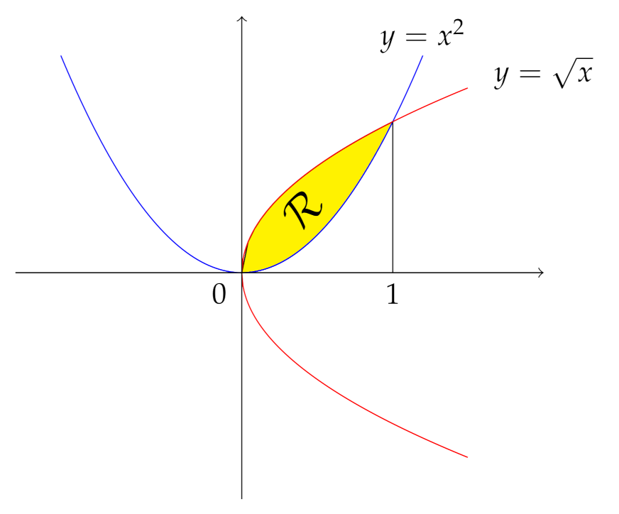
Figure 1. Region bounded by y = x 2 and y = x .
Mathematics 09 02866 g001
Figure 2. Region bounded by x 2 + y 2 = 2 a x ; x 2 + y 2 = 2 b x ; y = x and y = 0 .
Mathematics 09 02866 g002
Figure 3. Portion of sphere x 2 + y 2 + z 2 1 in the first octant x , y , z 0 .
Mathematics 09 02866 g003
Figure 4. Portion of the paraboloid z = x 2 + y 2 with 0 z 1 .
Mathematics 09 02866 g004
Publisher’s Note: MDPI stays neutral with regard to jurisdictional claims in published maps and institutional affiliations.