Convergence Analysis and Dynamical Nature of an Efficient Iterative Method in Banach Spaces

Abstract

We study the local convergence analysis of a fifth order method and its multi-step version in Banach spaces. The hypotheses used are based on the first Fréchet-derivative only. The new approach provides a computable radius of convergence, error bounds on the distances involved, and estimates on the uniqueness of the solution. Such estimates are not provided in the approaches using Taylor expansions of higher order derivatives, which may not exist or may be very expensive or impossible to compute. Numerical examples are provided to validate the theoretical results. Convergence domains of the methods are also checked through complex geometry shown by drawing basins of attraction. The boundaries of the basins show fractal-like shapes through which the basins are symmetric.

1. Introduction

Let X, Y be Banach spaces and $D\subseteq X$ be a closed and convex set. In this study, we locate a solution $x*$ of the nonlinear equation

$$G\left(x\right)=0,$$

(1)

where $G:D\subseteq X\to Y$ is a Fréchet-differentiable operator. In computational sciences, many problems can be written in the form of (1). See, for example, [1,2,3]. The solutions of such equations are rarely attainable in closed form. This is why most methods for solving these equations are usually iterative. The most well-known method for approximating a simple solution $x*$ of Equation (1) is Newton’s method, which is given by

$$x_{m+1}=x_m-G^{\prime }{\left(x_m\right)}^{-1}G\left(x_m\right),\mathrm{for}\mathrm{each}m=0,1,2,\dots$$

(2)

and has a quadratic order of convergence. In order to attain the higher order of convergence, a number of modified Newton’s or Newton-like methods have been proposed in the literature (see [2,3,4,5,6,7,8,9,10,11,12,13,14,15,16,17,18,19,20]) and references cited therein. In particular, Sharma and Kumar [18] recently proposed a fifth order method for approximating the solution of $G\left(x\right)=0$ using the Newton–Chebyshev composition defined for each $n=0,1,2,\dots$ by

$$\begin{array}{ccc}\hfill y_m& =& x_m-{\mathsf{\Gamma }}_{m}G\left(x_m\right),\hfill \\ \hfill z_m& =& y_m-{\mathsf{\Gamma }}_{m}G\left(y_m\right),\hfill \\ \hfill x_{m+1}& =& z_m-\left(2I-{\mathsf{\Gamma }}_n[z_m,y_m;G]\right){\mathsf{\Gamma }}_{m}G\left(z_m\right),\hfill \end{array}$$

(3)

where ${\mathsf{\Gamma }}_m=G^{\prime }{\left(x_m\right)}^{-1}$, and $[z_m,y_m;G]$ is the first order divided difference of G. The method has been shown to be computationally more efficient than existing methods of a similar nature.

The important part in the development of an iterative method is to study its convergence analysis. This is usually divided into two categories, namely the semilocal and local convergence. The semilocal convergence is based on the information around an initial point and gives criteria that ensure the convergence of iteration procedures. The local convergence is based on the information of a convergence domain around a solution and provides estimates of the radii of the convergence balls. Local results are important since they provide the degree of difficulty in choosing initial points. There exist many studies which deal with the local and semilocal convergence analysis of iterative methods such as [3,4,5,7,8,9,10,11,13,16,19,21,22,23]. The semilocal convergence of the method (3) in Banach spaces has been established in [18]. In the present work, we study the local convergence of this method and its multi-step version, including the computable radius of convergence, error bounds on the distances involved, and estimates on the uniqueness of the solution.

We summarize the contents of the paper. In Section 2, the local convergence (including radius of convergence, error bounds, and uniqueness results of method (3)) is studied. The generalized multi-step version is presented in Section 3. Numerical examples are performed to verify the theoretical results in Section 4. In Section 5, the basins of attractors are studied to visually check the convergence domain of the methods. Finally, some conclusions are reported in Section 6.

2. Local Convergence

The local convergence analysis of method (3) is presented in this section. Let $L_0>0$, $L>0$, $L_1>0$, and $M\ge 0$ be given parameters. It is convenient to generate some functions and parameters for the local convergence study that follows. Define function $g_1\left(t\right)$ on interval $[0,\frac{1}{L_0})$ by

$$g_1\left(t\right)=\frac{Lt}{2(1-L_{0}t)}$$

and parameter

$$r_1=\frac{2}{2L_0+L}<\frac{1}{L_0}.$$

(4)

Then, we have that $g_1\left(r_1\right)=1$ and $0\le g_1\left(t\right)\le 1$ for each $t\in [0,r_1)$. Moreover, define the function $g_2\left(t\right)$ and $h_2\left(t\right)$ on interval $[0,\frac{1}{L_0})$ by

$$g_2\left(t\right)=\left(1+\frac{M}{1-L_{0}t}\right)g_1\left(t\right)$$

and

$$h_2\left(t\right)=g_2\left(t\right)-1.$$

We have that $h_2\left(0\right)=-1<0$ and $h_2\left(r_1\right)=\frac{M}{1-L_0{r}_1}>0$. According to the intermediate value theorem, function $h_2\left(t\right)$ has zeros in the interval $(0,r_1)$. Denote such zeros by $r_2$. Finally, define functions $K\left(t\right)$, $g_3\left(t\right)$, and $h_3\left(t\right)$ on the interval $[0,\frac{1}{L_0})$ by

$$K\left(t\right)=1+\frac{1}{1-L_{0}t}\left(L_0+L_{1}t(g_2\left(t\right)+g_1\left(t\right))\right)t,$$

$$g_3\left(t\right)=\left(1+\frac{MK\left(t\right)}{1-L_{0}t}\right)g_2\left(t\right)$$

and

$$h_3\left(t\right)=g_3\left(t\right)-1.$$

We have that $h_3\left(0\right)=-1<0$ and $h_3\left(r_2\right)=\frac{MK\left(r_2\right)}{1-L_0{r}_2}>0$. According to the intermediate value theorem, function $h_3\left(t\right)$ has zeros in $(0,r_2)$. Denote such zeros by $r_3$ of function $h_3\left(t\right)$ in interval $[0,r_2)$. Set

$$r=\min \left\{r_i\right\},i=1,2,3.$$

(5)

Then, we obtain that

$$0<r\le r_1.$$

(6)

Then, for each $t\in [0,r)$

$$0\le g_1\left(t\right)\le 1,$$

(7)

$$0\le g_2\left(t\right)\le 1$$

(8)

and

$$0\le g_3\left(t\right)\le 1.$$

(9)

Let $U(v,\rho$) and $\overline{U}(v,\rho )$ symbolise the open and closed balls in X, with a radius $\rho >0$ and a centre $v\in X$.

Using the above notations, we then describe the local convergence analysis of method (3).

Theorem 1.

Suppose $G:D\subseteq X\to Y$ is a Fréchet-differentiable function. Let $[.,.;G]:X\times X\to L\left(Y\right)$ be the divided difference operator. Consider that there exist $x*\in D$, $L_0>0$, $L>0$, $L_1>0$, and $M\ge 1$, such that for each $x,y\in D$

$$G\left(x*\right)=0,G{\left(x*\right)}^{-1}\in L(Y,X),$$

(10)

$$\parallel G^{\prime }{\left(x*\right)}^{-1}\left(G^{\prime }\left(x\right)-G^{\prime }\left(x*\right)\right)\parallel \le L_0\parallel x-x*\parallel ,$$

(11)

$$\parallel G^{\prime }{\left(x*\right)}^{-1}\left(G^{\prime }\left(x\right)-G^{\prime }\left(y\right)\right)\parallel \le L\parallel x-y\parallel ,$$

(12)

$$\parallel G^{\prime }{\left(x*\right)}^{-1}{G}^{\prime }\left(x\right)\parallel \le M,$$

(13)

$$\parallel G^{\prime }{\left(x*\right)}^{-1}\left([x,y;G]-G^{\prime }\left(x*\right)\right)\parallel \le L_1(\parallel x-x*\parallel +\parallel y-x*\parallel ),$$

(14)

and

$$\overline{U}(x*,r)\subset D,$$

(15)

where r is defined by (5). Then, for each $m=0,1,\dots$, the sequence $\left\{x_m\right\}$ generated by method (3) for $x_0\in U(x*,r)-\left\{x*\right\}$ is well defined, stays in $U(x*,r)$, and converges to $x*$. Furthermore, the following estimates hold:

$$\parallel y_m-x*\parallel \le g_1(\parallel x_m-x*\parallel )\parallel x_m-x*\parallel <\parallel x_m-x*\parallel <r,$$

(16)

$$\parallel z_m-x*\parallel \le g_2(\parallel x_m-x*\parallel )\parallel x_m-x*\parallel <\parallel x_m-x*\parallel <r$$

(17)

and

$$\parallel x_{m+1}-x*\parallel \le g_3(\parallel x_m-x*\parallel )\parallel x_m-x*\parallel ,$$

(18)

where the “$g$” functions are defined previously. Furthermore, if there exists $T\in [r,\frac{2}{L_0})$ such that $\overline{U}(x*,T)\subset D$, then $x*$ is the only solution of $G\left(x\right)=0$ in $\overline{U}(x*,T)$.

Proof. 

We shall show the estimates (16)–(18) using mathematical induction. Using (4), (11), and the hypotheses $x_0\in U(x*,r)-\left\{x*\right\}$, we obtain that

$$\parallel G^{\prime }{\left(x*\right)}^{-1}\left(G\left(x_0\right)-G\left(x*\right)\right)\parallel \le L_0\parallel x_0-x*\parallel <L_{0}r<1.$$

(19)

It follows from (19) and the Banach Lemma [3] that $G^{\prime }{\left(x_0\right)}^{-1}\in L(Y,X)$ and

$$\parallel G^{\prime }{\left(x_0\right)}^{-1}{G}^{\prime }\left(x*\right)\parallel \le \frac{1}{1-L_0\parallel x_0-x*\parallel }<\frac{1}{1-L_{0}r}.$$

(20)

Hence, $y_0$ is well defined for $m=0$. Then, by using (4), (7), (12), and (20), we have

$$\begin{array}{cc}\hfill \parallel y_0-x*\parallel & \le \parallel x_0-x*-G^{\prime }{\left(x_0\right)}^{-1}G\left(x_0\right)\parallel \hfill \\ \hfill & \le \parallel G^{\prime }{\left(x_0\right)}^{-1}{G}^{\prime }\left(x*\right)\parallel \parallel {\int }_0^1{G}^{\prime }{\left(x*\right)}^{-1}[G^{\prime }(x*+\theta (x_0-x*))-G^{\prime }\left(x_0\right)]]\parallel d\theta \hfill \\ \hfill & \times \parallel x_0-x*\parallel \hfill \\ \hfill & \le \frac{L\parallel x_0-x*{\parallel }^2}{2(1-L_0\parallel x_0-x*\parallel )}\hfill \\ \hfill & =g_1(\parallel x_0-x*\parallel )\parallel x_0-x*\parallel <\parallel x_0-x*\parallel <r,\hfill \end{array}$$

(21)

which shows (16) for $m=0$ and $y_0\in U(x*,r)$.

Notice that for each $\theta \in [0,1]$ and $\parallel x*+\theta (x_0-x*)-x*\parallel =\theta \parallel x_0-x*\parallel <r$. That is, $x*+\theta (x_0-x*)\in U(x*,r)$. We can write

$$G\left(x_0\right)=G\left(x_0\right)-G\left(x*\right)={\int }_0^1{G}^{\prime }(x*+\theta (x_0-x*))(x_0-x*)d\theta .$$

(22)

Then, using (13) and (21), we have

$$\begin{array}{cc}\hfill \parallel G^{\prime }{\left(x*\right)}^{-1}G\left(x_0\right)\parallel & =\parallel {\int }_0^1{G}^{\prime }{\left(x*\right)}^{-1}{G}^{\prime }(x*+\theta (x_0-x*))(x_0-x*)d\theta \parallel \hfill \\ \hfill & \le M\parallel x_0-x*\parallel .\hfill \end{array}$$

(23)

Similarly, we obtain

$$\parallel G^{\prime }{\left(x*\right)}^{-1}G\left(y_0\right)\parallel \le M\parallel y_0-x*\parallel ,$$

(24)

$$\parallel G^{\prime }{\left(x*\right)}^{-1}G\left(z_0\right)\parallel \le M\parallel z_0-x*\parallel .$$

(25)

Using the second substep of method (3), (8), (20), (21), (27), and (24), we obtain that

$$\begin{array}{cc}\hfill \parallel z_0-x*\parallel \le & \parallel y_0-x*\parallel +\parallel G^{\prime }{\left(x_0\right)}^{-1}G\left(y_0\right)\parallel \hfill \\ \hfill =& \parallel y_0-x*\parallel +\parallel G^{\prime }{\left(x_0\right)}^{-1}{G}^{\prime }\left(x*\right)\parallel \parallel G^{\prime }{\left(x*\right)}^{-1}G\left(y_0\right)\parallel \hfill \\ \hfill \le & \parallel y_0-x*\parallel +\frac{M\parallel y_0-x*\parallel }{1-L_0\parallel x_0-x*\parallel }\hfill \\ \hfill \le & \left(1+\frac{M}{1-L_0\parallel x_0-x*\parallel }\right)\parallel y_0-x*\parallel \hfill \\ \hfill \le & \left(1+\frac{M}{1-L_0\parallel x_0-x*\parallel }\right)g_1(\parallel x_0-x*\parallel )\parallel x_0-x*\parallel \hfill \\ \hfill \le & g_2(\parallel x_0-x*\parallel )\parallel x_0-x*\parallel <\parallel x_0-x*\parallel <r.\hfill \end{array}$$

(26)

Which shows (17) for $m=0$ and $z_0\in U(x*,r)$.

Next, we have the linear operator $A_0=2I-G^{\prime }{\left(x_0\right)}^{-1}[y_0,x_0;G]$; by using (11), (14), and (20), we obtain

$$\begin{array}{cc}\hfill \parallel A_0\parallel & =\parallel 2I-G^{\prime }{\left(x_0\right)}^{-1}[z_0,y_0;G]\parallel \hfill \\ \hfill & \le 1+\parallel G^{\prime }{\left(x_0\right)}^{-1}\left(G^{\prime }\left(x_0\right)-[z_0,y_0;G]\right)\parallel \hfill \\ \hfill & \le 1+\parallel G^{\prime }{\left(x_0\right)}^{-1}{G}^{\prime }\left(x*\right)\parallel \parallel G^{\prime }{\left(x*\right)}^{-1}(G^{\prime }\left(x_0\right)-[z_0,y_0;G])\parallel \hfill \\ \hfill & \le 1+\parallel G^{\prime }{\left(x_0\right)}^{-1}{G}^{\prime }\left(x*\right)\parallel \parallel G^{\prime }{\left(x*\right)}^{-1}\left(G^{\prime }\left(x_0\right)-G^{\prime }\left(x*\right)+G^{\prime }\left(x*\right)-[z_0,y_0;G]\right)\parallel \hfill \\ \hfill & \le 1+\parallel G^{\prime }{\left(x_0\right)}^{-1}{G}^{\prime }\left(x*\right)\parallel \left(\parallel G^{\prime }{\left(x*\right)}^{-1}(G^{\prime }\left(x_0\right)-G^{\prime }\left(x*\right))\parallel +\parallel G^{\prime }{\left(x*\right)}^{-1}(G^{\prime }\left(x*\right)-[z_0,y_0;G])\parallel \right)\hfill \\ \hfill & \le 1+\frac{2}{1-L_0\parallel x_0-x*\parallel }\left(L_0\parallel x_0-x*\parallel +L_1\left(\parallel z_0-x*\parallel +\parallel y_0-x*\parallel \right)\right)\hfill \\ \hfill & \le 1+\frac{2}{1-L_0\parallel x_0-x*\parallel }\left(L_0\parallel x_0-x*\parallel +L_1\left(g_2(\parallel x_0-x*\parallel )+g_1(\parallel x_0-x*\parallel )\right)\parallel x_0-x*\parallel \right)\hfill \\ \hfill & \le 1+\frac{2}{1-L_0\parallel x_0-x*\parallel }\left(L_0+L_1\left(g_2(\parallel x_0-x*\parallel )+g_1(\parallel x_0-x*\parallel )\right)\right)\parallel x_0-x*\parallel \hfill \\ \hfill & =K(\parallel x_0-x*\parallel ).\hfill \end{array}$$

(27)

Then, using Equations (4), (9), (25), and (26), we obtain that 2.0

$$\begin{array}{cc}\hfill \parallel x_1-x*\parallel \le & \parallel z_0-x*\parallel +\parallel A_0\parallel \parallel G^{\prime }{\left(x_0\right)}^{-1}G\left(z_0\right)\parallel \hfill \\ \hfill =& \parallel z_0-x*\parallel +\parallel A_0\parallel \parallel G^{\prime }{\left(x_0\right)}^{-1}{G}^{\prime }\left(x*\right)\parallel \parallel G^{\prime }{\left(x*\right)}^{-1}G\left(z_0\right)\parallel \hfill \\ \hfill \le & \parallel z_0-x*\parallel +\frac{MK(\parallel x_0-x*\parallel )\parallel z_0-x*\parallel }{1-L_0\parallel x_0-x*\parallel }\hfill \\ \hfill \le & \left(1+\frac{MK(\parallel x_0-x*\parallel )}{1-L_0\parallel x_0-x*\parallel }\right)\parallel z_0-x*\parallel \hfill \\ \hfill \le & \left(1+\frac{MK(\parallel x_0-x*\parallel )}{1-L_0\parallel x_0-x*\parallel }\right)g_2(\parallel x_0-x*\parallel )\parallel x_0-x*\parallel \hfill \\ \hfill \le & g_3(\parallel x_0-x*\parallel )\parallel x_0-x*\parallel <\parallel x_0-x*\parallel <r,\hfill \end{array}$$

(28)

which proves the (18) for $m=0$ and $x_1\in U(x*,r)$. By simply replacing $x_0$, $y_0$, $z_0$, and $x_1$ by $x_m$, $y_m$, $z_m$, and $x_{m+1}$ in the preceding estimates, we arrive at (16)–(18). Then, from the estimates $\parallel x_{m+1}-x*\parallel <\parallel x_m-x*\parallel <r$, we deduce that ${lim}_{m\to \infty }{x}_m=x*$ and $x_{m+1}\in U(x*,r)$.

Finally, we show the uniqueness part; let $Q={\int }_0^1{G}^{\prime }(x*+t(x*-y^{*}))dt$ for some $y^{*}\in \overline{U}(x*,r)$ with $G\left(y^{*}\right)=0$. Using (15), we obtain that

$$\begin{array}{cc}\hfill \parallel G^{\prime }{\left(x*\right)}^{-1}(Q-G^{\prime }\left(x*\right)\parallel & \le {\int }_0^1{L}_0\parallel y*+t(x*-y*)-x*\parallel dt\hfill \\ \hfill & \le {\int }_0^1(1-t)\parallel x*-y*\parallel dt\hfill \\ \hfill & \le \frac{L_0}{2}T<1.\hfill \end{array}$$

(29)

It follows from (29) that Q is invertible. Then, from the identity $0=G\left(x*\right)-G\left(y*\right)=Q(x*-y*)$, we deduce that $x*=y*$. □

Remark 1.

By (11) and the estimate

$$\begin{array}{cc}\hfill \parallel G^{\prime }{\left(x*\right)}^{-1}{G}^{\prime }\left(x\right)\parallel & =\parallel G^{\prime }{\left(x*\right)}^{-1}(G^{\prime }\left(x\right)-G^{\prime }\left(x*\right))+I\parallel \hfill \\ \hfill & \le 1+\parallel G^{\prime }{\left(x*\right)}^{-1}(G^{\prime }\left(x\right)-G^{\prime }\left(x*\right))\parallel \hfill \\ \hfill & \le 1+L_0\parallel x-x*\parallel \hfill \end{array}$$

condition (13) can be dropped and be replaced by

$$M\left(t\right)=1+L_{0}t$$

or

$$M\left(t\right)=M=2,\mathit{since}t\in [0,\frac{1}{L_0}).$$

3. Generalized Method

The multistep version of (3) consisting of $q+1$, $(q\in \mathbb{N})$, steps is expressed as

$$\begin{array}{cc}\hfill & z_m^{\left(0\right)}=y_m-{\mathsf{\Gamma }}_{m}G\left(y_m\right),\hfill \\ \hfill & z_m^{\left(1\right)}=z_m-\psi (x_m,y_m,z_m)G\left(z_m\right),\hfill \\ \hfill & z_m^{\left(2\right)}=z_m^{\left(1\right)}-\psi (x_m,y_m,z_m)G\left(z_m^{\left(1\right)}\right),\hfill \\ \hfill & \dots \dots \dots \dots \dots \dots \hfill \\ \hfill & z_m^{(q-1)}=z_m^{(q-2)}-\psi (x_m,y_m,z_m)G\left(z_m^{(q-2)}\right),\hfill \\ \hfill & z_m^{\left(q\right)}=x_{m+1}=z_m^{(q-1)}-\psi (x_m,y_m,z_m)G\left(z_m^{(q-1)}\right),\hfill \end{array}$$

(30)

where $y_m=x_m-{\mathsf{\Gamma }}_{m}G\left(x_m\right)$, $z_m^{\left(0\right)}=z_m$, $\psi (x_m,y_m,z_m)=(2I-{\mathsf{\Gamma }}_m[z_m,y_m;G]){\mathsf{\Gamma }}_m$, and ${\mathsf{\Gamma }}_m=G{\left(x_m\right)}^{-1}$.

Next, we show that the generalized scheme (30) possesses convergence order $2q+3$.

3.1. Order of Convergence

The definition of divided difference is required to derive (30) convergence order. Recalling the result of Taylor’s expansion on vector functions (see [24]) for this:

Lemma 1.

$G:D\subset {\mathbb{R}}^n\to {\mathbb{R}}^n$ be r-times Fréchet differentiable in a convex set $D\subset {\mathbb{R}}^n$ then for any $x,h\in {\mathbb{R}}^n,$ the following expression holds:

$$\begin{array}{c}\hfill G(x+h)=G\left(x\right)+G^{\prime }\left(x\right)h+\frac{1}{2!}{G}^{″}\left(x\right)h^2+\frac{1}{3!}{G}^{‴}\left(x\right)h^3+\dots +\frac{1}{(r-1)!}{G}^{(r-1)}\left(x\right)h^{r-1}+R_r,\end{array}$$

(31)

where

$$\left|\right|R_r\left|\right|\le \frac{1}{r!}\underset{0\le t\le 1}{sup}\left|\right|G^{\left(r\right)}{(x+th)\left|\right|\left|\right|h\left|\right|}^{r}and{h}^r=(h,h,\stackrel{r}{\dots },h).$$

The divided difference operator $[·,·;G]:D\times D\subset {\mathbb{R}}^n\times {\mathbb{R}}^n⟶L\left({\mathbb{R}}^n\right)$ is defined by (see [24])

$$[x+h,x;G]={\int }_0^1{G}^{\prime }(x+th)dt,\forall x,h\in {\mathbb{R}}^n.$$

(32)

When we expand $G^{\prime }(x+th)$ in the Taylor series at point x and integrate, we obtain

$$[x+h,x;G]={\int }_0^1{G}^{\prime }(x+th)dt=G^{\prime }\left(x\right)+\frac{1}{2}{G}^{″}\left(x\right)h+\frac{1}{6}{G}^{‴}\left(x\right)h^2+O\left(h^3\right).$$

(33)

where $h^i=(h,h,\stackrel{i}{\dots },h),h\in {\mathbb{R}}^n.$

Let $e_m=x_m-x*$. Expanding $G\left(x_m\right)$ in a neighbourhood of $x*$ and assuming $\mathsf{\Gamma }=G^{\prime }{\left(x*\right)}^{-1}$ exists, we obtain

$$G\left(x_m\right)=G^{\prime }(x*)(e_m+A_2{\left(e_m\right)}^2+A_3{\left(e_m\right)}^3+A_4{\left(e_m\right)}^4+A_5{\left(e_m\right)}^5+O({\left(e_m\right)}^5)),$$

(34)

where $A_i=\frac{1}{i!}\mathsf{\Gamma }{G}^{\left(i\right)}\left(x*\right)\in L_i({\mathbb{R}}^n,{\mathbb{R}}^n)$ and ${\left(e_m\right)}^i=(e_m,e_m,\stackrel{i}{\dots },e_m),e_m\in {\mathbb{R}}^n,i=2,3,\dots$

Additionally,

$$G^{\prime }\left(x_m\right)=G^{\prime }\left(x*\right)(I+2A_2{e}_m+3A_3{\left(e_m\right)}^2+4A_4{\left(e_m\right)}^3+O({\left(e_m\right)}^4)),$$

(35)

$$G^{″}\left(x_m\right)=G^{\prime }(x*)(2A_2+6A_3{e}_m+12A_4{\left(e_m\right)}^2+O({\left(e_m\right)}^3)),$$

(36)

$$G^{‴}\left(x_m\right)=G^{\prime }\left(x*\right)(6A_3+24A_4{e}_m+O({\left(e_m\right)}^2)).$$

(37)

The inversion of $G^{\prime }\left(x_m\right)$ yields

$$\begin{array}{cc}\hfill G^{\prime }{\left(x_m\right)}^{-1}=(I& -2A_2{e}_m+(4A_2^2-3A_3){\left(e_m\right)}^2-(4A_4-6A_2{A}_3-6A_3{A}_2+8A_2^3){\left(e_m\right)}^3\hfill \\ \hfill & +O({\left(e_m\right)}^4))\mathsf{\Gamma }.\hfill \end{array}$$

(38)

We are in a position to investigate scheme (30)’s convergence behaviour. As a result, the following theorem is established:

Theorem 2.

Suppose that

(i) $G:D\subset {\mathbb{R}}^n\to {\mathbb{R}}^n$ is many times differentiable mapping.

(ii) There exists a solution $x*\in D$ of equation $G\left(x\right)=0$ such that $G^{\prime }\left(x*\right)$ is nonsingular.

Then, sequence $\left\{x_n\right\}$ generated by method (30) for $x_0\in D$ converges to $x*$ with order $2q+3$, $q\in \mathbb{N}$.

Proof. 

Employing (34) and (38) in the Newton iteration $y_m$, we obtain that

$$\begin{array}{cc}\hfill {\tilde{e}}_m=& y_m-x*=A_2{e}_m^2+(2A_2^2-A_3)e_m^3+(4A_2^3-4A_2{A}_3-3A_3{A}_2+3A_4)e_m^4\hfill \\ \hfill & -(8A_2^4+6A_3^2+6A_2{A}_4+4A_4{A}_2-8A_2^2{A}_3-6A_2{A}_3{A}_2-6A_3{A}_2^2)e_m^5+O\left(e_m^6\right).\hfill \end{array}$$

(39)

The Taylor series of $G\left(y_m\right)$ about $x*$ yields

$$G\left(y_m\right)=G^{\prime }\left(x*\right)({\tilde{e}}_m+A_2{\tilde{e}}_m^2+A_3{\tilde{e}}_m^3+A_4{\tilde{e}}_m^4+O\left({\tilde{e}}_m^5\right)),$$

(40)

Substituting (38)–(40) in first step of (30), we obtain

$$\begin{array}{c}\hfill {\overline{e}}_m=z_m-x*=2A_2^2{e}_m^3+(4A_2{A}_3-9A_2^3+3A_3{A}_2)e_m^4+O\left(e_m^5\right).\end{array}$$

(41)

Using Equations (35)–(37) in (33) for $x+h=z_m$, $x=y_m$, and $h={\overline{e}}_m-{\tilde{e}}_m$, it follows that

$$\begin{array}{c}\hfill [z_m,y_m;G]=G^{\prime }\left(x*\right)\left(I+A_2({\overline{e}}_m+{\tilde{e}}_m)+O({\left({\tilde{e}}_m\right)}^2,{\left({\overline{e}}_m\right)}^2)\right)\end{array}$$

and

$${\mathsf{\Gamma }}_m[z_m,y_m;G]=I-2A_2{e}_m+(4A_2^2-3A_3){\left(e_m\right)}^2+A_2({\overline{e}}_m+{\tilde{e}}_m)+O\left({\left(e_m\right)}^3\right).$$

As a result, we arrive at the conclusion

$$\begin{array}{c}\hfill \psi (x_m,y_m,z_m)=\left(I-5A_2^2{\left(e_m\right)}^2+2(10A_2^3-4A_2{A}_3-3A_3{A}_2){\left(e_m\right)}^3+O({\left(e_m\right)}^4))\right)G^{\prime }{\left(x*\right)}^{-1}.\end{array}$$

(42)

In addition, we have

$$G\left(z_m\right)=G^{\prime }\left(x*\right)({\overline{e}}_m+O({\left({\overline{e}}_m\right)}^2)).$$

(43)

Using (42) and (43) in the second step of method (30), it follows that

$$z_m^{\left(1\right)}-x*=10A_2^4{\left(e_m\right)}^5+O\left({(e_m)}^6\right).$$

(44)

The expansion of $G\left(z_m^{(q-1)}\right)$ about $x*$ yields

$$G\left(z_m^{(q-1)}\right)=G^{\prime }\left(x*\right)\left((z_m^{(q-1)}-x*)+A_2{(z_m^{(q-1)}-x*)}^2+\cdots \right).$$

(45)

Then, we have

$$\begin{array}{cc}\hfill \psi (x_m,y_m,z_m)G\left(z_m^{(q-1)}\right)=& \left(I-5A_2^2{\left(e_m\right)}^2+2(10A_2^3-4A_2{A}_3-3A_3{A}_2){\left(e_m\right)}^3+O\left({\left(e_m\right)}^4\right))\right)G^{\prime }{\left(x*\right)}^{-1}\hfill \\ \hfill & \times G^{\prime }\left(x*\right)\left((z_m^{(q-1)}-x*)+A_2{(z_m^{(q-1)}-x*)}^2+\cdots \right)\hfill \\ \hfill =& (z_m^{(q-1)}-x*)-5A_2^2(z_m^{(q-1)}-x*){\left(e_m\right)}^2+A_2{(z_m^{(q-1)}-x*)}^2+\dots .\hfill \end{array}$$

(46)

Using (46) in (30), we obtain

$$\begin{array}{c}\hfill z_m^{\left(q\right)}-x*=5A_2^2(z_m^{(q-1)}-x*){\left(e_m\right)}^2-A_2{(z_m^{(q-1)}-x*)}^2+\cdots .\end{array}$$

(47)

As we know from (44) that $z_m^{\left(1\right)}-x*=10A_2^4{\left(e_m\right)}^5+O\left({\left(e_m\right)}^6\right)$, from (47) for $q=2,3$, we therefore have

$$\begin{array}{cc}\hfill z_m^{\left(2\right)}-x*=& 5A_2^2{\left(e_m\right)}^2(z_m^{\left(1\right)}-x*)+\cdots \hfill \\ \hfill =& 50A_2^6{\left(e_m\right)}^7+O\left({\left(e_m\right)}^8\right)\hfill \end{array}$$

and

$$\begin{array}{cc}\hfill z_m^{\left(3\right)}-x*=& 5A_2^2{\left(e_m\right)}^2(z_m^{\left(2\right)}-x*)+\cdots \hfill \\ \hfill =& 250A_2^8{\left(e_m\right)}^9+O\left({\left(e_m\right)}^{10}\right).\hfill \end{array}$$

Proceeding by induction, it follows that

$$e_{m+1}=z_m^{\left(q\right)}-x*=2·5^q{A}_2^{2q+2}{\left(e_m\right)}^{2q+3}+O\left({\left(e_m\right)}^{2q+4}\right).$$

This completes the proof of Theorem 2. □

Remark 2.

Note that method (3) utilizes three functions, one derivative, and one inverse operator per full iteration and converges to the solution with the fifth order of convergence. The generalized scheme (30) based on (3) (for $q=1$) generates the methods with increasing convergence orders $5,7,9,\dots$ corresponding to $q=1,2,3,\dots$ at an additional cost of one function evaluation per each iteration. This fulfils the main aim of developing higher order methods, keeping computational cost under control.

3.2. Local Convergence

Along the same lines as method (3), we offer the local convergence analysis of method (30). Define ${\overline{g}}_2$, $\lambda$, $\mu$, and $h_{\mu }$ on the interval $[0,r_2)$ by

$${\overline{g}}_2\left(t\right)=\frac{K\left(t\right)}{1-w_0\left(t\right)},$$

$$\lambda \left(t\right)=1+{\overline{g}}_2\left(t\right)M,$$

$$\mu \left(t\right)={\lambda }^q\left(t\right)g_2\left(t\right)t^{\lambda -1}$$

and

$$h_{\mu }\left(t\right)=\mu \left(t\right)-1.$$

We have that $h_{\mu }\left(0\right)<0$. Suppose that

$$\mu \left(t\right)\to +\infty \mathrm{or}\mathrm{a}\mathrm{positive}\mathrm{number}\mathrm{as}t\to r_2^{-}.$$

(48)

Denote by $r^{\left(q\right)}$ the smallest zero on the interval $(0,r_2)$ of function $h_{\mu }$. Define $r*$ by

$$r*=\min \{r_1,r^{\left(q\right)}\}.$$

(49)

Proposition 1.

Suppose that the conditions of Theorem 2 hold. Then, sequence $\left\{x_m\right\}$ generated for $x_0\in U(x*,r*)-\left\{x*\right\}$ by method (30) is well defined in $U(x*,r*)$, remains in $U(x*,r*)$, and converges to $x*$. Moreover, the following estimates hold:

$$\begin{array}{cc}\hfill \parallel y_m-x*\parallel & \le g_1(\parallel x_m-x*\parallel )\parallel x_m-x*\parallel \le \parallel x_m-x*\parallel <r*,\hfill \\ \hfill \parallel z_m-x*\parallel & \le g_2(\parallel x_m-x*\parallel )\parallel x_m-x*\parallel \le \parallel x_m-x*\parallel ,\hfill \\ \hfill \parallel z_m^{\left(i\right)}-x*\parallel & \le {\lambda }^i(\parallel x_m-x*\parallel )\parallel z_m-x*\parallel \hfill \\ \hfill & \le {\lambda }^i(\parallel x_m-x*\parallel )g_2(\parallel x_m-x*\parallel )\parallel x_m-x*{\parallel }^{\lambda }\hfill \\ \hfill & \le \parallel x_m-x*\parallel ,i=1,2,\dots ,q-1,\hfill \end{array}$$

(50)

and

$$\begin{array}{cc}\hfill \parallel x_{k+1}-x*\parallel =\parallel z_m^{\left(q\right)}-x*\parallel & \le {\lambda }^q(\parallel x_m-x*\parallel )\parallel z_m-x*\parallel \hfill \\ \hfill & \le \mu (\parallel x_m-x*\parallel )\parallel x_m-x*\parallel .\hfill \end{array}$$

(51)

Furthermore, $x*$ is the only solution of $G\left(x\right)=0$ in $D_1=D\cap U(x*,r*)$.

Proof. 

Only new estimations (50) and (51) will be shown. We show the first two estimations using the evidence of Theorem 1. Then, we will be able to obtain that

$$\begin{array}{cc}\hfill \parallel \psi (x_m,y_m,z_m)G^{\prime }\left(x*\right)\parallel \le & \parallel \left(2I-G^{\prime }{\left(x_m\right)}^{-1}[z_m,y_m;G]\right)G^{\prime }{\left(x_m\right)}^{-1}{G}^{\prime }\left(x*\right)\parallel \hfill \\ \hfill \le & \parallel \left(2I-G^{\prime }{\left(x_m\right)}^{-1}[z_m,y_m;G]\right)\parallel \parallel G^{\prime }{\left(x_m\right)}^{-1}{G}^{\prime }\left(x*\right)\parallel \hfill \\ \hfill \le & \frac{K(\parallel x_m-x*\parallel )}{1-w_0(\parallel x_m-x*\parallel )}\hfill \\ \hfill \le & {\overline{g}}_2(\parallel x_m-x*\parallel ).\hfill \end{array}$$

(52)

Moreover, we have

$$\begin{array}{cc}\hfill \parallel z^{\left(1\right)}-x*\parallel & =\parallel z_m-x*-\psi (x_m,y_m)G\left(z_m\right)\parallel \hfill \\ \hfill & \le \parallel z_m-x*\parallel +\parallel \psi (x_m,y_m,z_m)G^{\prime }\left(x*\right)\parallel \parallel G^{\prime }{\left(x*\right)}^{-1}G\left(z_m\right)\parallel \hfill \\ \hfill & \le \parallel z_m-x*\parallel +{\overline{g}}_2(\parallel x_m-x*\parallel )M\parallel z_m-x*\parallel \hfill \\ \hfill & \le \lambda (\parallel x_m-x*\parallel )\parallel z_m-x*\parallel \hfill \\ \hfill & \le \mu (\parallel x_m-x*\parallel )\parallel x_m-x*\parallel .\hfill \end{array}$$

Similarly, we obtain

$$\begin{array}{cc}\hfill \parallel z_m^{\left(2\right)}-x*\parallel & \le \lambda (\parallel x_m-x*\parallel )\parallel z_m^{\left(1\right)}-x*\parallel \hfill \\ \hfill & \le {\lambda }^2(\parallel x_m-x*\parallel )\parallel z_m-x*\parallel \hfill \\ \hfill & \dots \dots \dots \dots \dots \dots \hfill \\ \hfill \parallel z_m^{\left(i\right)}-x*\parallel & \le {\lambda }^i(\parallel x_m-x*\parallel )\parallel z_m-x*\parallel \hfill \\ \hfill \parallel x_{m+1}-x*\parallel & \le \parallel z_m^{\left(q\right)}-x*\parallel \le {\lambda }^q(\parallel x_m-x*\parallel )\parallel z_m-x*\parallel \hfill \\ \hfill & \le \mu (\parallel x_m-x*\parallel )\parallel x_m-x*\parallel .\hfill \end{array}$$

That is, we have $x_m$, $y_m$,$z_m$, $z_m^{\left(i\right)}$$\in U(x*,r*)$, $i=1,2,\dots ,q$, and

$$\parallel x_{m+1}-x*\parallel \le \overline{c}\parallel x_m-x*\parallel ,$$

(53)

where $\overline{c}=\mu (\parallel x_0-x*\parallel )\in [0,1)$, so ${lim}_{m\to \infty }{x}_m=x*$ and $x_{m+1}\in U(x*,r*)$. The uniqueness result is standard, as shown in Theorem 1. □

4. Numerical Examples

Here, we shall demonstrate the theoretical results of local convergence which we have proved in Section 2 and Section 3. To do so, the methods of the family (30) of order five, seven, and nine are chosen. Let us denote these methods by $M_5$, $M_7$, and $M_9$, respectively. The divided difference in the examples is computed by $[x,y;F]={\int }_0^1{F}^{\prime }(y+\theta (x-y))d\theta$. We consider three numerical examples, which are presented as follows:

Example 1.

Let us consider $B={\mathbb{R}}^{m-1}$ for natural integer $m\ge 2$. B is equipped with the max-norm $\parallel x\parallel$$={\max }_{1\le i\le m-1}\parallel x_i\parallel$. The corresponding matrix norm is $\parallel A\parallel ={\max }_{1\le i\le m-1}{\sum }_{j=1}^{j=m-1}\left|a_{ij}\right|$ for $A=$${\left(a_{ij}\right)}_{1\le i,j\le m-1}$. Consider the two-point boundary value problem on interval [0, 1]:

$$\left\{\begin{array}{c}{v}^{″}+v^{3/2}=0,\hfill \\ v\left(0\right)=v\left(1\right)=0.\hfill \end{array}\right.$$

(54)

Let us denote $\Delta =1/m$, $u_i=\Delta i$, and $v_i=V\left(u_i\right)$ for each $i=0,1,\dots ,m$. We can write the discretization of $v^{{}^{″}}$ at points $u_i$ in the following form:

$$v_i^{{}^{″}}\simeq \frac{v_{i-1}-2v_i+v_{i+1}}{{\Delta }^2}\mathrm{for}\mathrm{each}i=2,3,\dots ,m-1.$$

Using the initial conditions in (54), we obtain that $v_0=v_m=0$, and (54) is equivalent to the system of the nonlinear equation $F\left(v\right)=0$ with $v=(v_1,v_2,\dots ,v_{m-1})$ in the following form:

$$\left\{\begin{array}{c}{\Delta }^2{v}_1^{3/2}-2v_1+v_2=0,\hfill \\ v_{i-1}+{\Delta }^2{v}_i^{3/2}-2v_i+v_{i+1}=0\mathrm{for}\mathrm{each}i=2,3,\dots ,m-1.\hfill \end{array}\right.$$

(55)

Using (55), the Fréchet-derivative of operator F is given by

$$F^{\prime }\left(v\right)=\left(\begin{array}{ccccc}\frac{3}{2}{\Delta }^2{v}_1^{1/2}-2& 1& 0& \dots & 0\\ 1& \frac{3}{2}{\Delta }^2{v}_1^{1/2}-2& 1& \ddots & 0\\ 0& 1& \ddots & \ddots & ⋮\\ ⋮& \ddots & \ddots & \ddots & 1\\ 0& \dots & 0& 1& \frac{3}{2}{\Delta }^2{v}_1^{1/2}-2\end{array}\right).$$

Choosing $m=11$, the corresponding solution is $x*={(0,0,0,0,0,0,0,0,0,0)}^T$, and we have $L_0=L=L_1=3.942631477$ and $M=2$. The parameters using method (30) are given in

Table 1. Numerical results for example 1.

${\mathit{M}}_5$	${\mathit{M}}_7$	${\mathit{M}}_9$
$r_1=0.00791011$	$r_1=0.00791011$	$r_1=0.00791011$
$r^{\left(1\right)}=0.00470691$	$r^{\left(2\right)}=8.50886\times {10}^{-10}$	$r^{\left(3\right)}=1.61122\times {10}^{-13}$
$r^{*}=0.00470691$	$r^{*}=8.50886\times {10}^{-10}$	$r^{*}=1.61122\times {10}^{-13}$

.

Thus, it follows that the above-considered methods of scheme (30) converge to $x*$ and remain in $\overline{U}(x*,r*)$.

Example 2.

Scholars have determined that the speed of blood in a course is an element of the distance of the blood from the conduit’s focal pivot (Figure 1). As per Poiseuille’s law, the speed (cm/s) of blood that is r cm from the focal hub of a supply route is given by the capacity

$$S\left(r\right)=C(R^2-r^2),$$

(56)

where R is the range of the course, and C is a consistent that relies upon the thickness of the blood and the tension between the two closures of the vein. Assume that for a specific course,

$$C=1.76\times {10}^5\mathrm{c}\mathrm{m}/\mathrm{s}$$

and

$$R=1.2\times {10}^{-2}\mathrm{c}\mathrm{m}.$$

Using the numerical values, the problem reduces to

$$f_2\left(x\right)=25.344-176,000x^2=0,$$

where $x=r$.

The graph of the function $f_2\left(x\right)$ is shown in Figure 2.

The zero of $f_2\left(x\right)=0$ is $x*=0.012$; then, we have $L_0=L=L_1=84.2803$ and $M=5280$. The parameters using method (30) are given in

Table 2. Numerical results for example 2.

${\mathit{M}}_5$	${\mathit{M}}_7$	${\mathit{M}}_8$
$r_1=0.169092$	$r_1=0.169092$	$r_1=0.169092$
$r^{\left(1\right)}=0.0724823$	$r^{\left(2\right)}=0.0331151$	$r^{\left(3\right)}=0.0140628$
$r^{*}=0.0724823$	$r^{*}=0.0331151$	$r^{*}=0.0140628$

.

It follows that the above-considered methods of scheme (30) will converge to $x*$ and remain in $\overline{U}(x*,r*)$ if $r*$ is chosen as shown in Table 2.

Example 3.

Consider the quasi-one-dimensional isentropic flow of a perfect gas through a variable-area channel, shown in Figure 3.

The relationship between the Mach number M and the flow area A, derived by Zucrow and Hoffman [25], is given by

$$\epsilon =\frac{A}{A^{*}}=\frac{1}{M}{\left(\frac{2}{\gamma +1}\left(1+\frac{\gamma -1}{2}{M}^2\right)\right)}^{(\gamma +1)/2(\gamma -1)},$$

(57)

where $A*$ is the choking area (i.e., the area where $M=1$), and $\gamma$ is the specific heat ratio of the flowing gas shown in Figure 4.

For each value of $\epsilon$, two values of M exist, one less than unity (i.e., subsonic flow) and one greater than unity (i.e., supersonic flow). For the values of $\epsilon =5.00$ and $\gamma =1.4$, Equation (57) becomes

$$f_3\left(x\right)=5-\frac{0.578704{(1+0.2x^2)}^3}{x}.$$

(58)

where $x=M$. The graph of the function $f_3\left(x\right)$ is shown in Figure 5, and the zero is $x*=0.116689$. Then, we have that

$$L=L_0=L_1=8.137146,\mathrm{and}M=0.610065.$$

The parameters using method (30) are given in

Table 3. Numerical results for example 3.

${\mathit{M}}_5$	${\mathit{M}}_7$	${\mathit{M}}_9$
$r_1=0.0819303$	$r_1=0.0819303$	$r_1=0.0819303$
$r^{\left(1\right)}=0.050974$	$r^{\left(2\right)}=0.0355748$	$r^{\left(3\right)}=0.0254287$
$r^{*}=0.050974$	$r^{*}=0.0355748$	$r^{*}=0.0254287$

.

The computed values of $r*$ show that the considered methods of the scheme (30) will converge to $x*$ and remain in $\overline{U}(x*,r*)$.

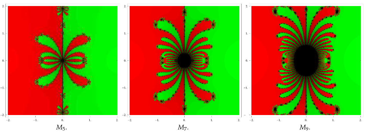
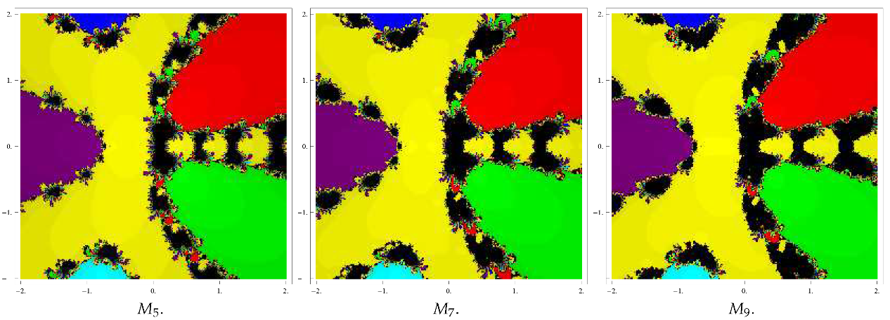
5. Study of Complex Dynamics of the Method

To view the geometry of the methods of the family (30) of five, seven, and nine order methods, in the complex plane, we present the attraction of basins of the roots by performing the methods on some functions (see

Table 4. Comparison of performance based on basins of attraction of methods.

S. No.	Test Problems	Roots	Color of Fractal	Best Performer	Poor Performer
1	$P_1\left(z\right)=z^2-4$	$-2$	red	$M_5$,	$M_7$, $M_9$
		2	green
2	$P_2\left(z\right)=z^3-z$	$-1$	red	$M_5$	$M_7$, $M_9$
		0	green
		1	blue
3	$P_3\left(z\right)=z^6+\frac{15}{7}{z}^5+5z^4$	$-0.8277\dots$	cyan	$M_5$, $M_7$	$M_9$
	$+\frac{7}{3}{z}^3-z^2+z+1$	$-0.7654-1.9514$i	yellow
		$-0.6562\dots$	purple
		$-0.7654+1.9514$i	blue
		$0.4357-0.4786$i	green
		$0.4357+0.4786$i	red

). The basins are displayed in Figure 6, Figure 7 and Figure 8 concerning capacities. To draw basins, we use square shapes $R\in \mathbb{C}$ of size $[-2,2]\times [-2,2]$ and allot various shadings to the basins. The dark region is appointed to the focuses for which the strategy is disparate.

6. Conclusions

In this work, we have extended the utilization of technique (3) by introducing its assembly investigation and complex elements. Rather than using different procedures depending on the higher subordinate request just as a Taylor series, we have utilized only a subsidiary of request one, since this actually shows up in the technique. One more benefit of our methodology is the calculation of uniqueness balls where the repeats lie just as appraisals on $\parallel x_n-x*\parallel$. These objectives are accomplished utilizing our Lipschitz-like conditions. The hypothetical outcomes so determined are confirmed on some useful issues. Finally, we have checked the security of the technique through utilizing a complex element apparatus, specifically a bowl of fascination.

References

1. Potra, F.-A.; Ptak, V. Nondiscrete Induction and Iterative Process, Research Notes in Mathematics; Pitman: Boston, MA, USA, 1984. [Google Scholar]
2. Traub, J.F. Iterative Methods for the Solution of Equations; Prentice-Hall: Englewood Cliffs, NJ, USA, 1964. [Google Scholar]
3. Argyros, I.K.; Hilout, S. Computational Methods in Nonlinear Analysis; World Scientific Publishing Company: Singapore, 2013. [Google Scholar]
4. Amat, S.; Hernández, M.A.; Romero, N. Semilocal convergence of a sixth order iterative method for quadratic equation. Appl. Num. Math. 2012, 62, 833–841. [Google Scholar] [CrossRef]
5. Argyros, I.K.; Ren, H. Improved local analysis for certain class of iterative methods with cubic convergence. Numer. Algor. 2012, 59, 505–521. [Google Scholar]
6. Argyros, I.K.; Regmi, S. Undergraduate Research at Cameron University on Iterative Procedures in Banach and Other Spaces; Nova Science Publisher: New York, NY, USA, 2019. [Google Scholar]
7. Argyros, I.K.; Sharma, J.R.; Kumar, D. Ball convergence of the Newton-Gauss method in Banach space. SeMA 2017, 74, 429–439. [Google Scholar] [CrossRef]
8. Babajee, D.K.R.; Dauhoo, M.Z.; Darvishi, M.T.; Barati, A. A note on the local convergence of iterative methods based on Adomian decomposition method and 3-node quadrature rule. Appl. Math. Comput. 2008, 200, 452–458. [Google Scholar] [CrossRef]
9. Candela, V.; Marquina, A. Recurrence relations for rational cubic methods I: The Halley method. Computing 1990, 44, 169–184. [Google Scholar] [CrossRef]
10. Candela, V.; Marquina, A. Recurrence relations for rational cubic methods II: The Chebyshev method. Computing 1990, 45, 355–367. [Google Scholar] [CrossRef]
11. Chun, C.; Stănică, P.; Neta, B. Third-order family of methods in Banach spaces. Comput. Math. Appl. 2011, 61, 1665–1675. [Google Scholar] [CrossRef] [Green Version]
12. Cordero, A.; Torregrosa, J.R. Variants of Newton’s method using fifth-order quadrature formulas. Appl. Math. Comput. 2007, 199, 686–698. [Google Scholar] [CrossRef]
13. Ezquerro, J.A.; Hernández, M.A. Recurrence relation for Chebyshev-type methods. Appl. Math. Optim. 2000, 41, 227–236. [Google Scholar] [CrossRef]
14. Usurelu, G.I.; Bejenaru, A.; Postolache, M. Newton-like methods and polynomiographic visualization of modified Thakur processes. Int. J. Comp. Math. 2021, 98, 1049–1068. [Google Scholar] [CrossRef]
15. Gdawiec, K.; Kotarski, W.; Lisowska, A. Polynomiography Based on the Nonstandard Newton-Like Root Finding Methods. Abst. Appl. Anal. 2015, 2015, 797594. [Google Scholar] [CrossRef] [Green Version]
16. Hasanov, V.I.; Ivanov, I.G.; Nebzhibov, F. A new modification of Newton’s method. Appl. Math. Eng. 2002, 27, 278–286. [Google Scholar]
17. Sharma, J.R.; Arora, H. On efficient weighted-Newton methods for solving systems of nonlinear equations. Appl. Math. Comput. 2013, 222, 497–506. [Google Scholar] [CrossRef]
18. Sharma, J.R.; Kumar, D. A fast and efficient composite Newton Chebyshev method for systems of nonlinear equations. J. Complex. 2018, 49, 56–73. [Google Scholar] [CrossRef]
19. Ren, H.; Wu, Q. Convergence ball and error analysis of a family of iterative methods with cubic convergence. Appl. Math. Comput. 2009, 209, 369–378. [Google Scholar] [CrossRef]
20. Weerkoon, S.; Fernado, T.G.I. A variant of Newton’s method with accelerated third-order convergence. Appl. Math. Lett. 2000, 13, 87–93. [Google Scholar] [CrossRef]
21. Hernández, M.A.; Salanova, M.A. Modification of Kantrovich assumptions for semi local convergence of Chebyshev method. J. Comput. Appl. Math. 2000, 126, 131–143. [Google Scholar] [CrossRef] [Green Version]
22. Gutiérrez, J.M.; Magreñán, A.A.; Romero, N. On the semilocal convergence of Newton-Kantrovich method under center-Lipschitz conditions. Appl. Math. Comput. 2013, 221, 79–88. [Google Scholar]
23. Kou, J.S.; Li, Y.T.; Wang, X.H. A modification of Newton’s method with third-order convergence. Appl. Math. Comput. 2006, 181, 1106–1111. [Google Scholar]
24. Ortega, J.M.; Rheinboldt, W.C. Iterative Solutions of Nonlinear Equations in Several Variables; Academic Press: New York, NY, USA, 1970. [Google Scholar]
25. Hoffman, J.D. Numerical Methods for Engineers and Scientists; McGraw-Hill Book Company: New York, NY, USA, 1992. [Google Scholar]
Figure 1. Cut-away view of an artery.
Mathematics 09 02510 g001
Figure 2. Graph of f 2 ( x ) .
Mathematics 09 02510 g002
Figure 3. In quasi-one-dimension flows, the stream tube cross section area is allowed to vary in one direction A = A ( x ) .
Mathematics 09 02510 g003
Figure 4. The area–Mach-number relation.
Mathematics 09 02510 g004
Figure 5. Graph of f 3 ( x ) .
Mathematics 09 02510 g005
Figure 6. Basins of attraction of M 5 , M 7 , and M 9 for polynomial P 1 ( z ) .
Mathematics 09 02510 g006
Figure 7. Basins of attraction of M 5 , M 7 , and M 9 for polynomial P 2 ( z ) .
Mathematics 09 02510 g007
Figure 8. Basins of attraction of M 5 , M 7 , and M 9 for polynomial P 3 ( z ) .
Mathematics 09 02510 g008