Article

Mixed Mesh Finite Volume Method for 1D Hyperbolic Systems with Application to Plug-Flow Heat Exchangers

by
Jiří Dostál
1,2,* and
Vladimír Havlena
1,2
1
Faculty of Electrical Engineering, Czech Technical University in Prague, Technická 2, 166 27 Prague, Czech Republic
2
University Centre for Energy Efficient Buildings, Czech Technical University in Prague, Třinecká 1024, 273 43 Buštěhrad, Czech Republic
*
Author to whom correspondence should be addressed.
Mathematics 2021, 9(20), 2609; https://doi.org/10.3390/math9202609
Submission received: 15 September 2021 / Revised: 7 October 2021 / Accepted: 8 October 2021 / Published: 16 October 2021
(This article belongs to the Special Issue Applications of Partial Differential Equations in Engineering)

Abstract

:
We present a finite volume method formulated on a mixed Eulerian-Lagrangian mesh for highly advective 1D hyperbolic systems altogether with its application to plug-flow heat exchanger modeling/simulation. Advection of sharp moving fronts is an important problem in fluid dynamics, and even a simple transport equation cannot be solved precisely by having a finite number of nodes/elements/volumes. Finite volume methods are known to introduce numerical diffusion, and there exist a wide variety of schemes to minimize its occurrence; the most recent being adaptive grid methods such as moving mesh methods or adaptive mesh refinement methods. We present a solution method for a class of hyperbolic systems with one nonzero time-dependent characteristic velocity. This property allows us to rigorously define a finite volume method on a grid that is continuously moving by the characteristic velocity (Lagrangian grid) along a static Eulerian grid. The advective flux of the flowing field is, by this approach, removed from cell-to-cell interactions, and the ability to advect sharp fronts is therefore enhanced. The price to pay is a fixed velocity-dependent time sampling and a time delay in the solution. For these reasons, the method is best suited for systems with a dominating advection component. We illustrate the method’s properties on an illustrative advection-decay equation example and a 1D plug flow heat exchanger. Such heat exchanger model can then serve as a convection-accurate dynamic model in estimation and control algorithms for which it was developed.

1. Introduction

Numerical computation is a fundamental tool for the study of complex phenomena described by sets of partial differential equations (PDE). Being able to simulate these equations gives the opportunity to answer not only research questions but to accelerate technological and knowledge advances in general. To name a few, numerical solutions of PDEs are important in fluid dynamics, magnetohydrodynamics, particle physics, automatic control, optimization, etc. In this paper, we deal with a class of problems arising in computational fluid dynamics, in particular, the advection-(diffusion)-reaction (ADR) equation. The ADR equation represents a variety of physical, chemical, or biological processes, where the examples include water pollution analysis, chemical reactors models, heat exchanger models, population growth, and others.
There exists countless amount of solution methods for such a system. Coarsely, one can choose from finite difference, finite element, or finite volume methods (FVM). Picking the FVM, which differs from the latter by engaging the divergence theorem, the main ingredients of the solutions are a spatial reconstruction scheme, numerical flux selection, grid (adaptation) selection, and a time integration method. Analysis of numerical methods for hyperbolic systems is given in [1].
A breakthrough paper by Godunov [2] presents a first-order upwind method and discusses the monotonicity of the solution schemes. Regarding spatial accuracy, his method is of the first order. A second-order scheme is referred to as MUSCL according to its originating paper [3]. This was also the first second-order total variation diminishing (TVD) [4] scheme. Such a property is there obtained by the use of a proper flux limiter function, e.g., minmod or superbee limiters [5]. There are, in fact infinitely many TVD flux limiter functions; they only need to fit the TVD region [6]. Arbitrary order, piecewise polynomial, essentially non-oscillatory scheme (ENO) for spatial reconstruction was presented in [7] and further developed in [8,9]. The most used nowadays, however, is the weighted essentially non-oscillatory scheme (WENO) first presented in [10] and further developed and analyzed in [11].
Numerical flux is driven by the Riemann problem solution, which can be either exact, e.g., [2], or approximate as in [12,13]. The latest development in the field focuses on adaptive mesh techniques. Moving mesh methods continuously reposition a finite number of grid points such that some measure is equalized over the grid; a review can be found in [14]. Another technique, the adaptive mesh refinement method, is, however, the most popular. Between the recent well-cited papers are [15,16], for example. Time integration is either multi-step, Runge–Kutta typically, or one-step, where the discontinuous Galerkin methods gain popularity lately.
This article presents a mixed-mesh method for a particular class of hyperbolic systems—systems with two characteristics, where one is non-zero and time-dependent. Traditional FVM may add significant artificial numerical diffusion at the low number of states/nodes; the presented mixed-mesh method eliminates this drawback. Sharp edges are convected undistorted even in low-dimensional situations, which is beneficial for control-oriented models for example. The model is given in the state-space representation for the convenience of the control community. Full implementation in Matlab is published as an open-source [17]. An exact discretization of the continuous model is prepared for a follow-up article.
The paper is organized as follows. First, the problem formulation is stated and a brief resume of FVM is given. The mixed-mesh finite volume method (MMFVM) is defined in the next section An application to a simple advection equation, together with a heat exchanger application, is presented at the end of the article.

1.1. Problem Formulation

Consider a general continuity equation in one spatial dimension
t q + x f = s ,
where the flux f x , t is of the form
f = V q + D q
and the variables of interest (states) q x , t : R × R R n are defined on a spatial domain x Ω and time domain t J , V t is a matrix of time-dependent transport velocities, D is a diffusion coefficient matrix, s q , x , t R n is a source/sink term and t = / t , x = / x are shorthand notations for partial differential operators with respect to time and space (Euler notation), respectively.
Under the assumption of an incompressible fluid, spatially invariant transport velocity and constant diffusion coefficients, we get a common advection-diffusion-reaction equation
t q + V x q + D x 2 q = s .
Focusing further on highly advective systems (with the Péclet number much larger than 10) the diffusion term is marginal and can be omitted [18]. Consider now the initial boundary value problem (IBVP) for the system (3), where q 0 x is an initial spatial profile at time t = t 0 and boundary conditions at x = 0 are b t (transport velocities are considered non-negative in the positive direction of x),
t q + V x q = s
q x , t 0 = q 0 x
q 0 , t = b t .
The goal is to obtain a transient solution for the variables q x , t on a defined time interval J t 0 , T . In particular, to obtain a numerical solution that preserves the wave behavior of the system without introducing numerical diffusion.

1.2. Finite Volume Method

Finite volume method (FVM) is one of the numerical solution techniques used for solving fluid dynamics problems. The core of the method lies in the usage of the divergence theorem on cells of finite volume and then on an approximation of the cell boundary fluxes from cell averages (a cell-centered method is assumed). More specifically, define a grid of N nodes, equidistant for simplicity, with a node to node distance Δ x = 1 / N . For any h : R × R R n define a notation of an average value over one grid length,
h ¯ x t = 1 Δ x c x h s , t d s ,
where the interval c x = x Δ x / 2 , x + Δ x / 2 . Now, applying the cell average to (3) and using the divergence theorem results in a system of ordinary differential equations for all cell-average variables
d d t q i + V Δ x q i 1 / 2 q i + 1 / 2 = s i ,
where q i = q ¯ x i is a cell average about position x i = i 1 / 2 Δ x , i = 1 , , N , q i ± 1 / 2 = q x i ± Δ x / 2 , t denote left and right face values, and s i = s ¯ x i is a cell source term average. The face value approximation depends on a numerical scheme used. In the first-order upwind scheme, for example, are the face values simply q i 1 / 2 = q i 1 , q i + 1 / 2 = q i . The first-order upwind approximation is monotone (no non-physical oscillations) but introduces a considerable numerical diffusion. Higher-order schemes bring higher accuracy, where the solution is smooth, but by the order barrier theorem, see [2] cannot be monotone. The remedy is to approximate the face values by a low order scheme, where the solution has high gradients, and by a high order scheme, where the solution is smooth. The switch between schemes is performed according to a slope/flux limiter function, and the method coined the term MUSCL [3]. Numerous limiters were introduced over the past five decades, starting with Van Leer [19]. An important class of slope limiters is the one forbidding an appearance of any new local extrema-the total variation diminishing class [4]. In the MUSCL scheme, the face values are approximated, component-wise, as
q i 1 / 2 = q i 1 + ϕ r i 1 2 q i 1 q i 2 q i + 1 / 2 = q i + ϕ r i 2 q i q i 1 ,
where the slope limiter function is, for example, the one by Van Leer [19]
ϕ r = r + r 1 + r
and the smoothness monitor is
r i = q i q i 1 q i + 1 q i .
See [20,21] for more schemes and slope limiters.
Time evolution of (5) is obtained using standard integration techniques such as RK4; special care, however, has to be taken concerning the sampling period. To contain the physical domain of dependence in the numerical domain of dependence (or in other words avoid interaction of adjacent Riemann problems), the sampling period must satisfy the Courant–Friedrichs–Lewy (CFL) condition [22]
max eig V Δ t Δ x .

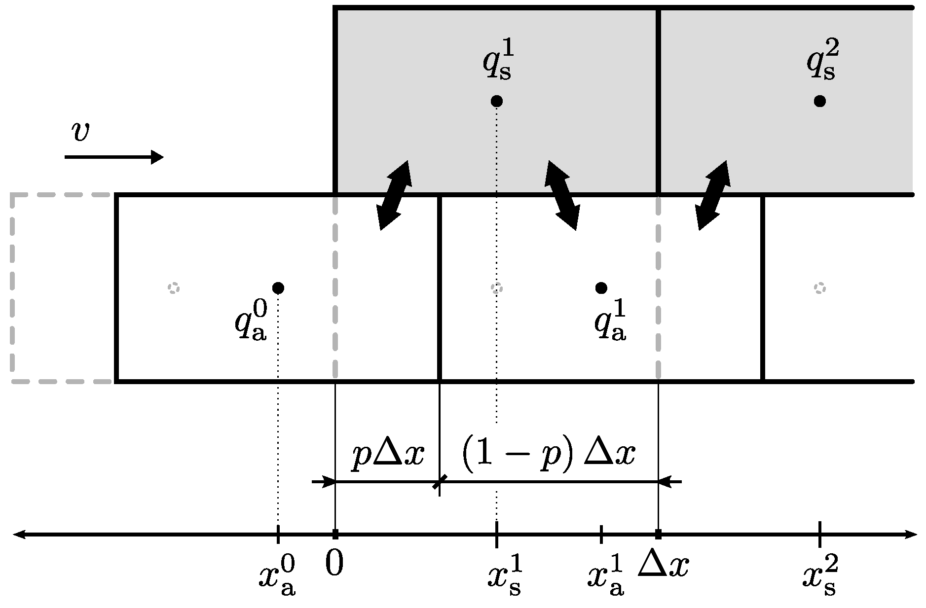
2. Mixed Mesh Finite Volume Method

The challenge of the numerical approximation of hyperbolic transport equations is to obtain high accuracy of the solution in both discontinuous and smooth regions [23]. Highly advective systems also present a challenge for the finite volume method. The cells are considered coherent (ideally mixed), and as a consequence, the flux at one boundary immediately influences fluxes at all the other boundaries. The numerical propagation speed is therefore always infinite for FVM. Pure discontinuities, as well, always dissolve into smooth step changes. The finer the grid, the less the phenomenon is observed. An exact solution, advecting discontinuities sharp, is obtained for an infinite number of cells [24].
To overcome this fundamental limitation, we propose a modified approach.
Remark 1.
Where coherent cells of finite volumes are used, an exact finite transport speed is only preserved by moving the grid by this velocity.
A Mixed-mesh Finite Volume Method (MMFVM) based on the observation of Remark 1 is presented here. The underlying principle is simple: advect (move) cells of the flowing field and simultaneously solve FVM for both the moving and static cells until the moving grid passes the static grid by one grid length; sample the state and reinitialize all moving cells to their starting positions and assign appropriate cell averages. The idea was first introduced in preceding conference papers of the authors [25,26] and will be generalized here. We believe a similar approach was used in [27,28], but a description of the spatially discretized system and its analysis are missing therein.
Definition 1 (Monocharacteristic hyperbolic system).
A system of the form (1), where the flux Jacobian J f / q can be decomposed to
J = v R D R 1 , D = diag d 1 , , d n , d i 0 , 1 i
with v t R being (for this paper) a space-independent velocity and R being a square decomposition matrix, is a monocharacteristic hyperbolic system, i.e., the system has a monocharacteristic hyperbolic property.
Remark 2.
As a hyperbolic system has a diagonalizable flux Jacobian with real eigenvalues a system is monocharacteristic hyperbolic when the Jacobian has just one nonzero eigenvalue, i.e., when a subset of the vector variable   q   advects with a transport (characteristic) velocity v, and the rest of q is stationary.
Definition 2 (Normal monocharacteristic form).
A normal monocharacteristic form is
t q + v I · · 0 x q = s
or equivalently
t q a q s + v I · · 0 x q a q s = s a s s ,
where q = q a T q s T T , s = s a T s s T T and q a x , t : R × R R n a is a vector of advected states, q s x , t : R × R R n s is a vector of stationary states and   s a q , u , t R n a , s s q , u , t R n s are respective spatially independent sink/source terms. I , 0 are square unit and zero matrices of appropriate sizes and · denotes rectangular zero matrix of coresponding size.
Lemma 1.
A system (1) with a monocharacteristic property (8) has a normal monocharacteristic form (9), (10).
Proof. 
We will prove the statement by transformation construction. The system (1) can be decomposed using the chain rule as
t q + f q x = const . x q = s x f q = const . ,
where J f / q x = const . is the flux Jacobian and s ¯ s / x f q = const . is an equivalent sink/source term. As the system is monocharacteristic hyperbolic, J can be decomposed to form (8). Defining now a permutation matrix P such that
P T D P = I · · 0 ,
the Jacobian is
J = v R P I · · 0 R P 1 .
So (1) can be rewritten as
t q + v R P I · · 0 R P 1 x q = s ¯ R P 1 t q + v I · · 0 R P 1 x q = R P 1 s ¯ .
Now, define a transformation T x = R P 1 x , then q ˜ T q , s ˜ T s ¯ and
t q ˜ + v I · · 0 x q ˜ = s ˜
is in a normal monocharacteristic form (9). □

Method Formulation

Consider a problem (1) with a monocharacteristic property (8) without a loss of generality in the monocharacteristic form (10)
t q a + v x q a = s a q a , q s , u
t q s = s s q a , q s , u
q a 0 , t = b t
q a x , 0 = q a , 0 x
q s x , 0 = q s , 0 x ,
where u t are external inputs, initial spatial profiles for advected states and static states are q a , 0 x , q s , 0 x , respectively and v t 0 . Define an equidistant grid of N elements with a grid spacing Δ x . The stationary grid Ξ s resembles the one of FVM
Ξ s = x s i i Z , 0 i N , Δ x = 1 N , x s i = i 1 2 Δ x ,
but the advected grid differs importantly. The basic idea behind the MMFVM is to allow the grid of advected states to flow along the stationary states with the characteristic velocity v.
Definition 3 (Relative cell shift).
A relative stationary-to-advected grid shift p is a distance a tracer would travel with a velocity v in a time interval t 0 , t 0 + τ taken relative to one grid length Δ x
p t = 1 Δ x t 0 t 0 + τ v s d s ,
where the integration start t 0 will be specified later on.
Definition 4 (Advected grid).
Grid positions of the advected states are
Ξ a = x a i i Z , 0 i N , x a i = x s i + p Δ x ,
where p is given by (13).
Remark 3.
Note that there is always at least one upwind “ghost” cell for the advected states at position x a 0 = p 1 / 2 Δ x , where a boundary condition is applied. Other ghost cells are added depending on the boundary conditions. See Figure 1 for illustration. Note that there is also a ghost cell at position x s 0 that can be used to apply boundary conditions for static states, but this cell in this paper does not play any role and is only added for future use and simplification of the notation.
Theorem 1 (MMFVM step).
Time evolution of a problem (11) discretized on grids Ξ s , Ξ a , is on a time interval t 0 , t 0 + τ given by
d d t q a i q s i = 1 p s a q a i , q s i , u s s q a i , q s i , u
+ p s a q a i , q s i + 1 , u s s q a i 1 , q s i , u
d d t p = v Δ x ,
where q a i , q s i , i = 0 , , N , denote centered cell average values of the advective and static grid, respectively, and s a q a 0 , q s 0 , u = 0 , s a q a N , q s N + 1 , u = 0 , s s q a 0 , q s 0 , u = 0 , s s q a 1 , q s 0 , u = 0 . The length of the time interval τ is given by the relative cell shift to integrate from p t 0 = 0 to p t 0 + τ = 1 or equivalently
t 0 t 0 + τ v t d t = Δ x .
The initial conditions are
q a i t 0 = q a x , t 0 x s i ¯
q s i t 0 = q s x , t 0 x s i ¯
p t 0 = 0 ,
for i = 1 , , N . The boundary conditions are applied to the upwind ghost cell   q a 0 t 0 = b t 0 at the beginning of the integration.
Proof. 
Direct. Spatial discretization of (11), by applying cell average operator (4) about positions x s i , x a i , gives
t q a ¯ x a i + v x q a ¯ x a i = s a ¯ x a i
t q s ¯ x s i = s s ¯ x s i
and to prove Theorem 1 we will deal with all the terms in (19) and (20) separately. Remember that x a i t = x s i + p t Δ x .
The time differential term (19) reads as
t q a ¯ x a i = 1 Δ x x a i t Δ x 2 x a i t + Δ x 2 t q a x , t d x ,
where using the Leibnitz’s integral rule the order of integration and differentiation can be switched to obtain
t q a ¯ x a i = 1 Δ x d d t x a i t Δ x 2 x a i t + Δ x 2 q a x , t d x 1 Δ x q a x a i t Δ x 2 , t d d t x a i t Δ x 2 + 1 Δ x q a x a i t + Δ x 2 , t d d t x a i t + Δ x 2 .
Now, first calculating the integral bounds derivative,
d d t x a i t ± Δ x 2 = d d t x s i + p t Δ x = Δ x d d t p t = Δ x d d t t 0 T v s Δ x d s = v t ,
we obtain the first term as
t q a ¯ x a i = 1 Δ x Δ x d d t q a i v q a i + 1 / 2 q a i 1 / 2 = d d t q a i v Δ x q a i + 1 / 2 q a i 1 / 2 ,
where q a i t = q a x a i ¯ t is a cell average value and q a i ± 1 / 2 t q a x a i ± Δ x / 2 , t denote cell face values.
The transport term (19) reads as
v x q a ¯ x a i = 1 Δ x x a i Δ x 2 x a i + Δ x 2 v x q a x , t d x ,
which using the Ostrogradsky’s divergence theorem simplifies to
v x q a ¯ x a i = v Δ x q a i + 1 / 2 q a i 1 / 2 .
The time differential term (20) reads as
t q s ¯ x s i = 1 Δ x x s i Δ x 2 x s i + Δ x 2 t q s x , t d x
which by substitution q s i t = q s ¯ x s i t immediately gives
t q s ¯ x s i = d d t q s i .
The static state source term (20) reads as
s s ¯ x s i = 1 Δ x x s i Δ x 2 x s i + Δ x 2 s s q a x , t , q s x , t , u t d x .
Given s s is spatially independent and inspecting Figure 1 we observe, that the integral may be separated as
s s ¯ x s i = 1 Δ x x s i Δ x 2 x s i Δ x 2 + p t Δ x s s q a x , t , q s x , t , u t d x + x s i Δ x 2 + p t Δ x x s i + Δ x 2 s s q a x , t , q s x , t , u t d x ,
which, under a piecewise constant spatial profile approximation of q a , q s is
s s ¯ x s i = 1 p s s q a i , q s i , u + p s s q a i 1 , q s i , u
and finally following the same reasoning as above we obtain the advected state source term (19)
s a ¯ x a i = 1 p s a q a i , q s i , u + p s a q a i , q s i + 1 , u .
The source term formulas are only valid for 0 p t 1 , which corresponds with (17). Note that higher order spatial reconstructions are possible following that appropriate calculation of the source terms (24), (25) above is performed.
Now, by substitution of (21) to (25) into (19), (20) we get
d d t q a i v Δ x q a i + 1 / 2 q a i 1 / 2 + v Δ x q a i + 1 / 2 q a i M M 1 / 2 = 1 p s a q a i , q s i , u + p s a q a i , q s i + 1 , u d d t q s i = 1 p s s q a i , q s i , u + p s s q a i 1 , q s i , u
moreover, we see that the velocity-dependent terms cancel out, and by aggregation of states, we obtain (15). Differentiation of the relative cell shift Equation (13),
d d t p t = v t Δ x
with p t 0 = 0 gives (16) and concludes the statement. □
Corollary 1 (MMFVM step for systems with a linear source term).
If a monocharacteristic hyperbolic system of Theorem 1 has a linear source term
s q a , q s , u = A aa A as A sa A ss q a q s + B a B s u ,
then (15) simplifies to
d d t q a i q s i = A aa A as A sa A ss q a i q s i + + p 0 A as A sa 0 q a i 1 q a i q s i + 1 q s i + + B a B s u
and the whole system of equations can be formulated as
d d t x = A c + p A cp x + B c u ,
where the state vector x R N + 1 · n aggregates the advected states and stationary states as
x = q a 0 T , , q a N T , q s 0 T , , q s N T T .
Proof. 
By construction. Substituting (26) into (15), after minor arrangements, gives (27). Defining now A ˜ c , 1 A aa A as A sa A ss , A ˜ c , 2 0 0 A sa 0 , A ˜ c , 3 0 A as 0 0 , B ˜ c B a B s , M = N + 1 and aggregating the states as
x ˜ = q a 0 T q s 0 T T , , q a N + 1 T q s N + 1 T T T ,
we can summarize (27) for i = 0 , , M into a formula
d d t x ˜ = I M A ˜ c , 1 x ˜ + p K 1 M A ˜ c , 2 + K + 1 M A ˜ c , 3 x ˜ + 1 M I n B ˜ c u ,
where K 1 M = I 1 M I M , K + 1 M = I + 1 M I M , I k denotes an identity matrix of size R k × k , I 1 k , I + 1 k are lower and upper shift matrices of size R k × k , respectively, 1 k R k is a column vector of ones and ⊗ denotes the Kronecker product. Now, define a permutation matrix P such that x = P T x ˜
P = P ˜ 1 2 , P ˜ = { p i , j } = 1 i odd , j = i + 1 2 1 i even , j = i + 2 N 2 0 otherwise ,
then (29) becomes (28) with
A c = P T I M A ˜ c , 1 P
A cp = P T K 1 M A ˜ c , 2 + K + 1 M A ˜ c , 3 P
B c = P T 1 M I n B ˜ c .
Theorem 2 (Mixed Mesh Finite Volume Method, MMFVM).
A numerical solution to a monocharacteristic hyperbolic system is obtained by a repetitive solution of the MMFVM step (Theorem 1/ Corollary 1).
There is a delay τ in the solution
τ i t : t τ i t t v s d s = Δ x 2 ; x = x s i , i = 1 , , N t τ i t t v s d s = Δ x ; x = x s i , i = N + 1
caused by the fact that there is an additional N + 1 st cell in the advected grid.
Proof. 
During the MMFVM step, the cell average values evolve by the governing PDE, as proved in the Theorem 1. Consider now a ghost cell q a 0 initialized by an appropriate boundary condition. It takes N + 1 MMFVM steps to move this cell along all the stationary cells. Only after N + 1 MMFVM steps, the cell has interacted with all the stationary cells and its value stops evolving.
The solution delay of the cell inside the spatial domain ( x = x s i , i = 1 , , N ) is caused by a length the MMFVM solution has to travel further opposed to a true analytic solution. More precisely, the true analytic residence time ς T i x , t is by the method of characteristics given as
ς T i x s i , t : t ς T i t v s d s = x s i = i 1 2 Δ x .
The MMFVM solution, however, has to travel a longer path (see Figure 1) and its residence time ς A i x , t is given by
ς A i x s i , t : t ς A i t v s d s = x s i + Δ x 2 = i Δ x ,
which can be, due to linearity of the integral operator, also written as
t ς A i t ς A i + ς T i v s d s + t ς A i + ς T i t v s d s = i 1 2 Δ x + Δ x 2 .
Defining a solution delay as τ i t = ς A i t ς T i t and identifying (33) in (34) we conclude the first part of (32)
t τ i t t v s d s = Δ x 2 , i = 1 , , N .
Similarly, for i = N + 1 , the analytic residence time ς T N + 1 is given by
t ς T N + 1 t v s d s = 1 .
The MMFVM residence time ς A N + 1 is given by
t ς A N + 1 t v s d s = N + 1 1 2 Δ x + Δ x 2 = 1 + Δ x ,
from which we can, by the same manipulation as above, conclude the remaining part of (32)
t τ N + 1 t t v s d s = Δ x .
Corollary 2 (State jump).
When a consecutive MMFVM step is being initialized (at p t = 1 from the preceding step), then the initial averaging of states (18) over the stationary grid Ξ s (instead of the fully shifted Ξ a grid) effectively performs a state shift/jump
q a i t + = q a i 1 t
q s i t + = q s i t
p t + = 0 ,
where t + denotes the just-after-jump instance at time t. Note that this relation holds only for a piecewise constant spatial profile approximation. Analogous relations can be derived for higher-order reconstructions.
Proof. 
Integration of (18) at p = 1 gives (35). See Figure 2 for illustration.
Note that in the case of a simple transport equation t q + v x q = s q , s q = A q + b , the solution delay (32) of MMFVM for the position x s N + 1 (corresponding to the analytic solution at x = 1 ) can be compensated by a modification to the velocity v ^ = N + 1 / N v and modification to the source term s ^ q = N + 1 / N A q + b . This statement can be shown to be true, but as it does not apply to the more general case considered, the proof is omitted.
Remark 4.
There is a minor numerical diffusion caused by the cell homogeneity (constant spatial profile over a cell). Imagine an advected cell being halfway shifted p = M M 1 / 2 , as it interacts with its left stationary cell, its state value changes and this, by cell homogeneity, in turn, affects the interaction with its right stationary cell and vice versa. This effect is, however, minor compared to FVM, where the cell homogeneity affects the greater advective flux.
In FVM, the sampling in time is bounded by the CFL condition (and possibly other stability conditions), but otherwise can be chosen freely. Sampling instances t k in MMFVM are, however, rigidly defined by the grid refinement and the actual characteristic velocity; in particular by
t 0 t 0 + t k v t d t = k Δ x , k N .
Those are the instances where the stationary and advected grid, (12) and (14), coincide, and when the last advected cell is done interacting with the stationary cell, and its value remains unchanged from thereon. The advected state boundary condition is sampled at this rate. Homogeneity assumption (piecewise constant spatial profile reconstruction) disallows free time sampling at fixed spatial positions due to passing discontinuities. Free time sampling is in general possible, but the quality of the solution strongly depends on the quality of the spatial profile reconstruction.
When the characteristic velocity tends to zero, the sampling intervals tend to infinity; this is not a desired property. To prevent this scenario, the following step is advised.
Remark 5.
When the sampling interval exceeds an allowed threshold, switch the solution method to FVM, i.e., stop the advected grid and incorporate the advective flux as is usual in FVM. It may also be beneficial to momentarily refine the grid.
Note that for low velocities the relative importance of the advective flux decreases and any numerical advection artifacts of FVM decrease. Also, as the velocity increases, the solution delay of MMFVM decreases. The MMFVM method is in a sense complementary to FVM, and its advantages prevail in highly advective scenarios.
Remark 6.
For systems with no static grid, apply the boundary condition directly to the first advected cell (and the upwind cells in the case of boundary conditions on the derivatives). MMFVM reduces to a system of ODEs with state shifts and solves the problem without transport delays in the solution.
Remark 7.
The (11) can be imagined as time and spatial evolution of an infinite number of infinitesimally small slices/points. For illustration, in a cooled water pipe, we can imagine infinitely many slices of water of width dx traveling by a defined input velocity through a pipe consisting again of infinitely many, now static, slices. For increasing N, MMFVM approximates ever so closely the continuum of the governing PDE; the solution delay of Theorem 2 diminishes and so does the numerical diffusion introduced in Remark 4.

3. Application

Two examples will be given; a simple transport-decay equation, for which an analytic solution is known and a plug-flow heat exchanger, for which comparison to a fine FVM solution will validate the solution.

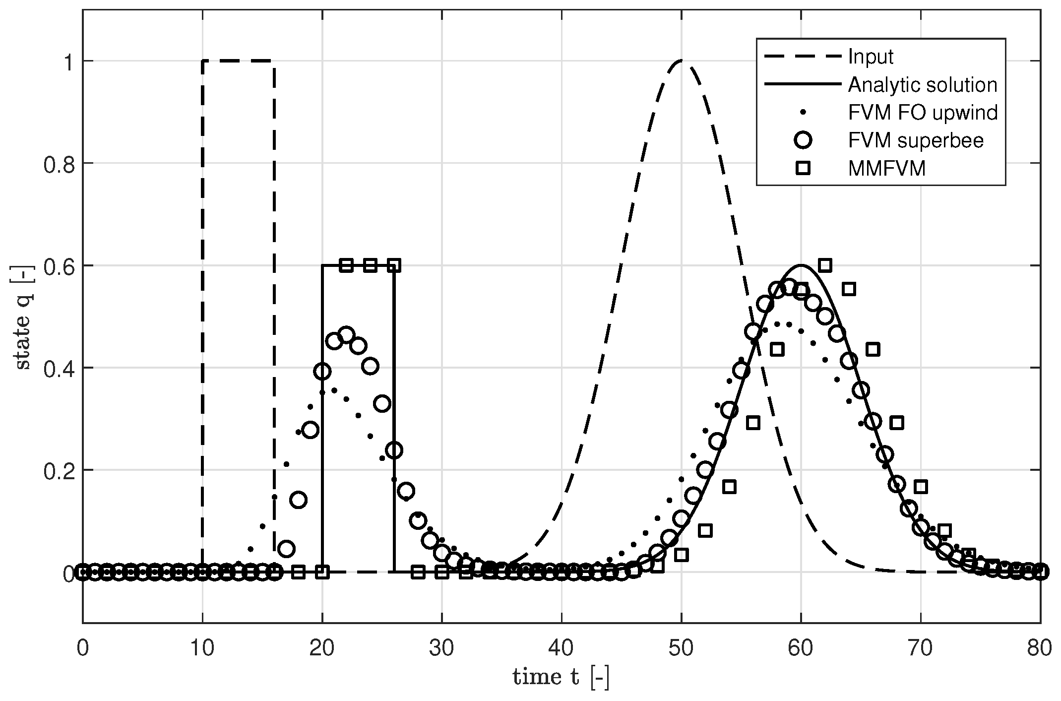
3.1. Advection-Decay Test

A simple transport equation with decay
t q x , t + v x q x , t = s q x , t q 0 , t = b t q x , 0 = 0
has by the method of characteristics an analytical solution that is only a time-shifted initial or boundary condition with exponential decay along the transport,
q x , t = 0 t < x v b t x v e s v x t x v .
This analytic solution is compared to an FVM solution with a first order upwind scheme, an FVM solution with a superbee limiter [5] and finally to the MMFVM.
According to the Theorem 2, the MMFVM solution is obtained by repetitive solution of the MMFVM step, i.e., integrate the following system in time
d d t q = s q d d t p = N v
for p 0 , 1 and perform a state jump according to Remark 2 at p = 1 , when b t is assigned to the first volume state.
Figure 3 shows the results for q 1 , t , with a simulation setting N = 5 , v = 0 . 1 and s = v ln 0 . 6 . A number of elements N = 5 is set low to highlight low-dimensional behavior of the said methods. Time integration is performed by BS23 [29] method with event location [30] (at p = 1 ). The analytic solution is q 1 , t = 0 . 6 × b t 10 , t 10 .  Figure 3 also contains the input signal b t .
It is noticeable that the FVM solution with first-order profile approximation brings great numerical diffusion to the solution. The usage of superbee slope limiter [5] improves the behavior, but under-performs in advecting discontinuities. The MMFVM solution is capable of truly advecting the input. The sampling is, however, dictated by the advection speed and is rather sparse in the case of only a few elements ( N = 5 ). Solution preserves the shape of input but suffers from the solution delay as analyzed in Theorem 2 and its proof.
Note that the problem contains no static states and therefore Remark 6 applies. However, to highlight properties of the method for general scenarios, the boundary condition has been applied to a first upwind ghost cell to generate the transport delay in the solution (N+1 integration steps instead of N). The source term had to be altered as s = s N N + 1 to account for this modification.

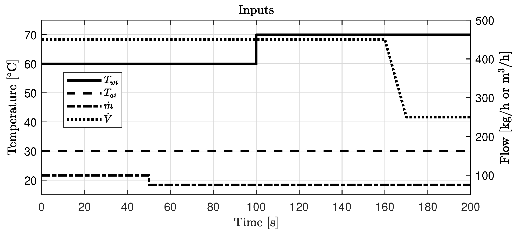
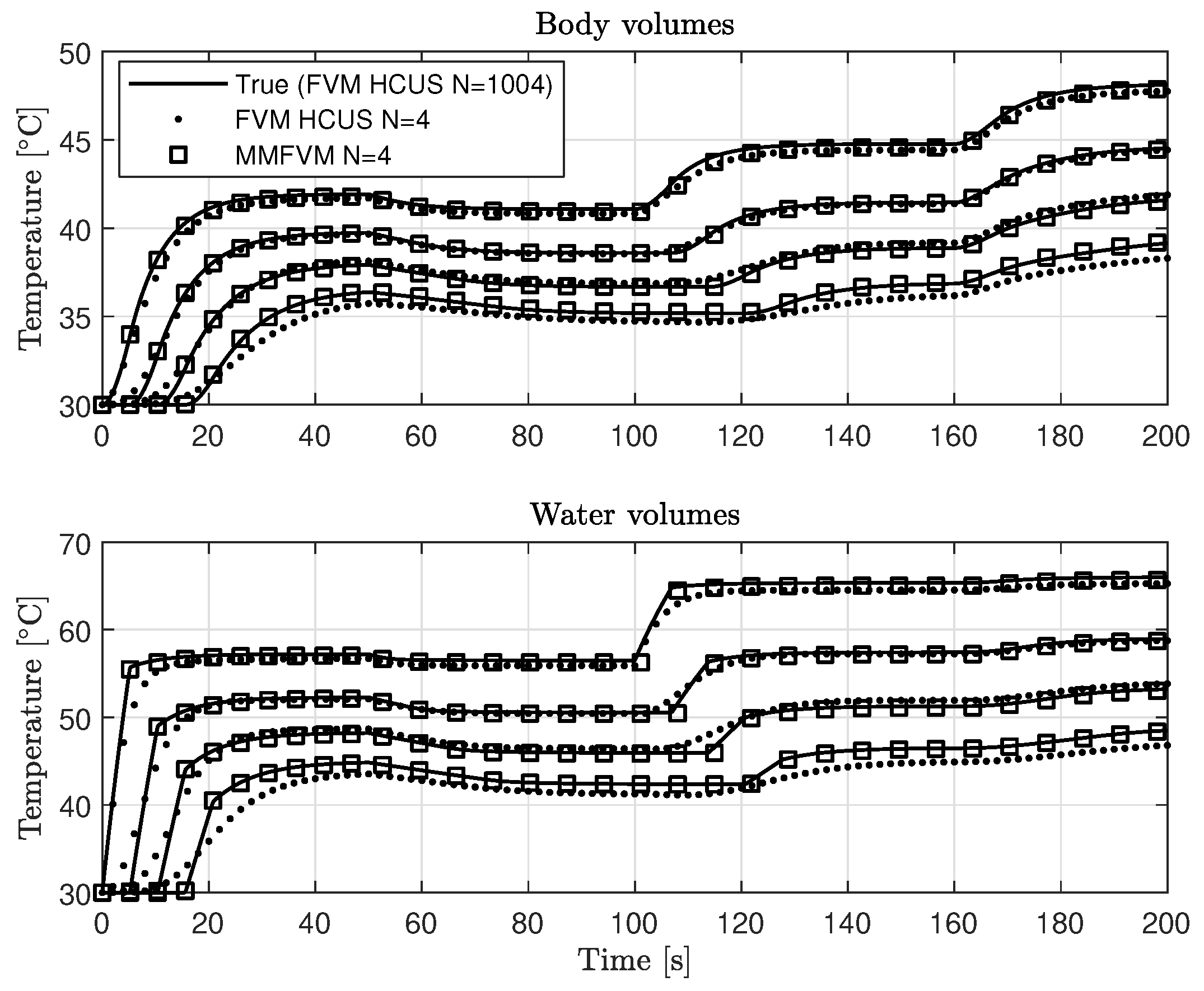
3.2. Water-to-Air Heat Exchanger Model

A plug flow heat exchanger is a plug flow reactor, where no reaction, only a heat exchange, occurs. Its model captures a distributed parameter, distributed time delay behavior and can be used for simplified modeling of, for example, water-to-air heat exchangers.
A water-to-air heat exchanger is considered to be a tubular single-pass cross-flow heat exchanger with the following assumptions: a 1 Heat transfer rates are constant in space, time and temperature. They solely depend on flow velocities. a 2 There is only one phase in both fluids, i.e., no condensation nor evaporation occurs. a 3 Fluids are incompressible and of constant density and specific heat capacity. a 4 Heat conduction (dispersion, diffusion) in the direction of flow is negligible. a 5 Water flow is radially coherent. The heat exchanger is thin in the air flow direction. a 6 Air flow has no dynamics and is ideally mixed at the inlet and outlet. The air temperature acting an the heat exchanger body as assumed constatnt and equal to the air inlet temperature. a 7 Water velocity (mass flow) is known.
The model is derived using the Fourier’s and conservation laws. The resulting system of partial differential equations is the first order hyperbolic
t T w + v x T w = α T b T w t T b = β 1 T w T b + β 2 T a T b ,
where the state variables T w = T w x , t ° C and T b = T b x , t ° C denote the water and metal body temperature, respectively, and v t = m ˙ t / m w s 1 is a normalized transport speed, where m ˙ kg / s is a water mass flow and m w kg a weight of water in the heat exchanger. The space variable was normalized using x = ξ / L , where ξ m is the space variable along the length of the heat exchanger, L m denotes the length of the heat exchanger.
The boundary conditions are
T w t , 0 = T w , in t T a t , x = T a , in t , x 0 , 1
moreover, initial conditions are
T w 0 , x = T w , 0 x T b 0 , x = T b , 0 x , x 0 , 1
where T w , 0 x and T b , 0 x are initial temperature profiles in the water and body, respectively, and T w , in t , T a , in t ° C are water and air inlet temperatures, respectively. The coefficients are
α = H wb m ˙ C w , β 1 = H wb m ˙ C b , β 2 = H ba V ˙ C b ,
where H wb m ˙ W / K , H ba ( V ˙ ) W / K are flow dependent heat exchange coefficients and C w J / K , C b J / K are total heat capacities of water and metal body, respectively. Air volumetric flow is denoted V ˙ m 3 / s . The outputs of the model are a heat flow from body to air Q t = 0 1 U A ba T b x , t T a , in t d x W and an outlet water temperature T w , out t = T w 1 , t .
FVM is applied in a standard way; the CFL condition is m ˙ t τ s t N m w , where τ s t is a sampling period.
For the application of MMFVM, first define advected and static state variables q a = T w , q s = T b and boundary conditions b t = T w , in t , u t = T a , in t . Quick observation of the source terms
s a q a , q s = α q a + α q s s s q a , q s = β 1 q a β 1 + β 2 q s + β 2 u ,
reveals their linearity. By application of the MMFVM step (26) we get the following evolution of volume averages
d d t q a i q s i = α α β 1 β 1 + β 2 q a i q s i + p 0 α β 1 0 q a i 1 q a i q s i + 1 q s i + 0 β 2 u
and a relative shift equation
d d t p = v Δ x .
Solving now this system according to Theorem 2 we obtain the solution. Time integration is performed by BS23 [29] method with event location [30] at p = 1 .
Setting of the experiment was: H wb m ˙ = 43 . 1 m ˙ / 3600 0 . 292 W / K ,   H ba V ˙ = 1 . 68 × 10 3 V ˙ 2 0 . 87 V ˙ + 260 W / K , C w = 2 . 41 · 10 3 J / K , C b = 2 . 26 × 10 3 J / K , m w = 0 . 577 kg , T w , 0 = T b , 0 = 20 ° C . The time sequence of all the four inputs is depicted in Figure 4. Figure 5 shows body and water volume temperatures at four equidistant spatial positions x = 0 . 125 , 0 . 375 , 0 . 625 , 0 . 875 (from top to bottom). Fine FVM solution ( N = 1004 ) with HCUS limiter [31] mimics the role of the true solution. To have a comparison with the two consecutive solutions with N = 4 , the states of the fine solution are averaged in space over Δ x = 1 / 4 . Figure 6 depicts the outputs. An interesting comparison begins with the FVM simulation with only four volumes ( N = 4 ) and HCUS flux limiter. Both state and output figures show how numerical diffusion alters the solution. The inlet temperature step at t = 100 s is smeared out, whereas the true solution is a sharp moving front. MMFVM with only four volumes ( N = 4 ) can advect the sharp front. However, the time sampling is tightly defined by the problem setting and transport velocity, as also is the solution delay. Considerable quality enhancement is achieved by having more volumes, a low number of volumes has been chosen to intensify the distinction in properties of the compared methods. Nevertheless, the MMFVM still performs reasonably well in this highly convective scenario.

4. Conclusions

A numerical solution method for systems with dominant advective components has been presented. The method utilized the Eulerian grid for stationary states and the Lagrangian grid for states with a characteristic velocity. Formulation of the interaction of the two grids is the main contribution of the paper. The employment of the Lagrangian grid removes advection flux from the cell-to-cell flux for its volumes as derived in the proof to Theorem 1. The solution to this problem formulation can contain discontinuities and a numerical diffusion is significantly decreased. As no finite numerical method can give an absolutely accurate numerical solution, there also is a price to pay for MMFVM. The time sampling intervals are advection velocity dependent, and there is a velocity-dependent delay in the solution. It is reasonable to resort to classic FVM for low-to-zero velocities, where diffusion/dispersion/conduction begin to prevail anyway. The MMFVM method should be used as complementary to FVM in highly-advective conditions Pe 10 . A low-order convection-accurate heat exchanger simulation model has been a primary motivation for the development of the method. The model has been implemented and its performance analyzed.

Author Contributions

Conceptualization, methodology, software, validation, formal analysis, writing—original draft preparation, writing—review and editing, visualization done by J.D.; supervision and proofreading provided by V.H. All authors have read and agreed to the published version of the manuscript.

Funding

This research was funded by Technology Agency of the Czech Republic grant number TK01020024 and by the Grant Agency of the Czech Technical University in Prague grant number SGS19/174/OHK3/3T/13.

Institutional Review Board Statement

Not applicable.

Informed Consent Statement

Not applicable.

Acknowledgments

We would like to kindly thank Vaclav Prajzner for the fruitful discussions during method conceptualization.

Conflicts of Interest

The authors declare no conflict of interest.

References

  1. Godlewski, E.; Raviart, P.A. Numerical Approximation of Hyperbolic Systems of Conservation Laws; Applied Mathematical Sciences 118; Springer: New York, NY, USA, 1996. [Google Scholar] [CrossRef]
  2. Godunov, S.K. A difference method for numerical calculation of discontinuous solutions of the equations of hydrodynamics. Mat. Sb. 1959, 89, 271–306. [Google Scholar]
  3. Van Leer, B. Towards the ultimate conservative difference scheme. V. A second-order sequel to Godunov’s method. J. Comput. Phys. 1979, 32, 101–136. [Google Scholar] [CrossRef]
  4. Harten, A. High resolution schemes for hyperbolic conservation laws. J. Comput. Phys. 1983, 49, 357–393. [Google Scholar] [CrossRef] [Green Version]
  5. Roe, P.L. Characteristic-based schemes for the Euler equations. Annu. Rev. Fluid Mech. 1986, 18, 337–365. [Google Scholar] [CrossRef]
  6. Sweby, P.K. High resolution schemes using flux limiters for hyperbolic conservation laws. SIAM J. Numer. Anal. 1984, 21, 995–1011. [Google Scholar] [CrossRef]
  7. Harten, A.; Engquist, B.; Osher, S.; Chakravarthy, S.R. Uniformly high order accurate essentially non-oscillatory schemes, III. J. Comput. Phys. 1987, 71, 231–303. [Google Scholar] [CrossRef]
  8. Shu, C.W.; Osher, S. Efficient implementation of essentially non-oscillatory shock-capturing schemes. J. Comput. Phys. 1988, 77, 439–471. [Google Scholar] [CrossRef] [Green Version]
  9. Shu, C.W.; Osher, S. Efficient implementation of essentially non-oscillatory shock-capturing schemes, II. J. Comput. Phys. 1989, 83, 32–78. [Google Scholar] [CrossRef]
  10. Liu, X.D.; Osher, S.; Chan, T. Weighted Essentially Non-oscillatory Schemes. J. Comput. Phys. 1994, 115, 200–212. [Google Scholar] [CrossRef] [Green Version]
  11. Jiang, G.S.; Shu, C.W. Efficient implementation of weighted ENO schemes. J. Comput. Phys. 1996, 126, 202–228. [Google Scholar] [CrossRef] [Green Version]
  12. Roe, P.L. Approximate Riemann solvers, parameter vectors, and difference schemes. J. Comput. Phys. 1981, 43, 357–372. [Google Scholar] [CrossRef]
  13. Toro, E.F.; Spruce, M.; Speares, W. Restoration of the contact surface in the HLL-Riemann solver. Shock Waves 1994, 4, 25–34. [Google Scholar] [CrossRef]
  14. Tang, T. Moving mesh methods for computational fluid dynamics. Contemp. Math. 2005, 383, 141–174. [Google Scholar] [CrossRef] [Green Version]
  15. Dumbser, M.; Zanotti, O.; Hidalgo, A.; Balsara, D.S. ADER-WENO finite volume schemes with space-time adaptive mesh refinement. J. Comput. Phys. 2013, 248, 257–286. [Google Scholar] [CrossRef] [Green Version]
  16. Buchmüller, P.; Dreher, J.; Helzel, C. Finite volume WENO methods for hyperbolic conservation laws on cartesian grids with adaptive mesh refinement. Appl. Math. Comput. 2016, 272, 460–478. [Google Scholar] [CrossRef]
  17. Dostal, J. MMFVM-HX-Model; GitHub: San Francisco, CA, USA, 2021. [Google Scholar] [CrossRef]
  18. Scott, A.; Socolofsky, G.H.J. CVEN 489-501: Special Topics in Mixing and Transport Processes in the Environment; Texas A&M University: College Station, TX, USA, 2005. [Google Scholar]
  19. Van Leer, B. Towards the ultimate conservative difference scheme. II. Monotonicity and conservation combined in a second-order scheme. J. Comput. Phys. 1974, 14, 361–370. [Google Scholar] [CrossRef]
  20. Wouwer, A.V.; Saucez, P.; Vilas, C. Simulation of ODE/PDE Models with MATLAB, OCTAVE and SCILAB; Springer: Berlin/Heidelberg, Germany, 2014. [Google Scholar] [CrossRef]
  21. Versteeg, H.K.; Malalasekera, W. An Introduction to Computational Fluid Dynamics: The Finite Volume Method, 2nd ed.; Pearson Education Limited: London, UK, 2007. [Google Scholar]
  22. Courant, R.; Friedrichs, K.; Lewy, H. On the partial difference equations of mathematical physics. IBM J. Res. Dev. 1967, 11, 215–234. [Google Scholar] [CrossRef]
  23. Jakobsen, H.A. Chemical Reactor Modeling; Springer International Publishing: Cham, Switzerland, 2014. [Google Scholar] [CrossRef]
  24. Dullemond, C.P.; Johansen, A. Numerical methods and applications. In Lecture Hydrodynamics; Heidelberg University: Heidelberg, Germany, 2007. [Google Scholar]
  25. Dostál, J.; Havlena, V. Convection oriented heat exchanger model. In Proceedings of the 2016 12th IEEE International Conference on Control and Automation (ICCA), Kathmandu, Nepal, 1–3 June 2016; pp. 347–352. [Google Scholar] [CrossRef]
  26. Dostál, J.; Prajzner, V.; Havlena, V. Convection oriented heat exchanger model—Identification. In Proceedings of the CLIMA 2016—12th REHVA World Congress, Aalborg, Denmark, 22–25 May 2016; Heiselberg, P.K., Ed.; Aalborg University: Aalborg, Denmark, 2016; Volume 9, pp. 1–8. [Google Scholar]
  27. Shang, H.; Forbes, J.F.; Guay, M. Characteristics-based model predictive control of distributed parameter systems. In Proceedings of the 2002 American Control Conference, Anchorage, AK, USA, 8–10 May 2002; Volume 6, pp. 4383–4388. [Google Scholar] [CrossRef]
  28. Shang, H.; Forbes, J.F.; Guay, M. Model predictive control for quasilinear hyperbolic distributed parameter systems. Ind. Eng. Chem. Res. 2004, 43, 2140–2149. [Google Scholar] [CrossRef]
  29. Bogacki, P.; Shampine, L.F. A 3(2) pair of Runge - Kutta formulas. Appl. Math. Lett. 1989, 2, 321–325. [Google Scholar] [CrossRef] [Green Version]
  30. Shampine, L.F.; Thompson, S. Event location for ordinary differential equations. Comput. Math. Appl. 2000, 39, 43–54. [Google Scholar] [CrossRef] [Green Version]
  31. Waterson, N.P.; Deconinck, H. A unified approach to the design and application of bounded higher-order convection schemes. Numer. Methods Laminar Turbul. Flow 1995, 9, 203–214. [Google Scholar]
Figure 1. Illustration of the advected grid movement against the static grid.
Mathematics 09 02609 g001
Figure 2. Illustration of a discrete state jump in otherwise continuous state evolution.
Mathematics 09 02609 g002
Figure 3. Method comparison for the advection-decay test at x = 1; number of volumes for all methods is N = 5.
Mathematics 09 02609 g003
Figure 4. Time sequence of inlet water temperature Tw,in, inlet air temperature Ta,in, water mass flow m ˙ and air volumetric flow V ˙ .
Mathematics 09 02609 g004
Figure 5. Time evolution of the body and water temperatures Tb, Tw at x = [0.125, 0.375, 0.625, 0.875] (from top to bottom). The fine FVM solution was spatially averaged to the cell size of the latter two solutions.
Mathematics 09 02609 g005
Figure 6. Time evolution of the heat output Q and the water outlet temperature Tw,out (at x = 1).
Mathematics 09 02609 g006
Publisher’s Note: MDPI stays neutral with regard to jurisdictional claims in published maps and institutional affiliations.

