Adaptive Boundary Control for a Certain Class of Reaction–Advection–Diffusion System

Abstract

Several phenomena in nature are subjected to the interaction of various physical parameters, which, if these latter are well known, allow us to predict the behavior of such phenomena. In most cases, these physical parameters are not exactly known, or even more these are unknown, so identification techniques could be employed in order to estimate their values. Systems for which their inputs and outputs vary both temporally and spatially are the so-called distributed parameter systems (DPSs) modeled through partial differential equations (PDEs). The way in which their parameters evolve with respect to time may not always be known and may also induce undesired behavior of the dynamics of the system. To reverse the above, the well-known adaptive boundary control technique can be used to estimate the unknown parameters assuring a stable behavior of the dynamics of the system. In this work, we focus our attention on the design of an adaptive boundary control for a parabolic type reaction–advection–diffusion PDE under the assumption of unknown parameters for both advection and reaction terms and Robin and Neumann boundary conditions. An identifier PDE system is established and parameter update laws are designed following the certainty equivalence approach with a passive identifier. The performance of the adaptive Neumann stabilizing controller is validated via numerical simulation.

1. Introduction

A large number of physical phenomena in nature can be modeled by partial differential equations (PDEs) like those in the field of engineering, physics, or chemical sciences since these disciplines encompass the study of phenomena such as electromagnetic field, acoustics, fluid flow, heat transfer, strength of materials, chemical reactions and concentration, mechanical vibrations, among other like logistics, flocking behavior, or even disease spreading. These phenomena have interactions between different variables and parameters for which it becomes necessary to correlate them into a mathematical model through the use of fundamental laws of nature, like those about conservation of energy, mass, and momentum. Due to the interaction between variables and parameters and by the way in which they vary both temporally and spatially, such processes are known as distributed parameter systems (DPSs). An essential feature of the DPSs is that they are infinite-dimensional systems that lead to PDEs for which, in some scenarios, it is possible to use a reduction methodology to transform the system into a finite-dimensional ordinary differential equation (ODE) in order to simplify the DPS making it more accurate for a specific application.

The PDEs are classified into three main categories, namely, the parabolic type, elliptic type, and hyperbolic type, according to the properties that each equation may have. Each one of these latter are used to describe the behavior of different phenomena, e.g., parabolic PDEs mainly describe heat transfer and diffusion processes, elliptic PDEs describe steady state behavior for systems like electrostatic fields, and the hyperbolic type are associated with vibrations or wave phenomena [1]. Unlike an ODE, where the solution leads to finding a specific state, the solution from a PDE lead us to find a family of functions due to its infinite-dimensional nature becoming necessary to establish certain conditions that help us to find the family of solutions inside a domain; such conditions are the so-called boundary conditions, namely, Dirichlet, Neumann, and Robin conditions, which ensures the well-posedness of the PDE [2].

In many DPSs, the physical parameters are unknown because these vary as the dynamics of the system evolve over time. From control theory, a recurrent approach has been widely used for estimation of unknown parameters from finite-dimensional systems, namely, the adaptive control technique, which has been extended to the control of infinite-dimensional PDEs. The adaptive control technique for PDEs successfully contribute to estimating the unknown parameters assuring the convergence to their true values. Depending on the location of the sensors and actuators, the control of PDEs can be performed either in the domain or at the boundary.

Some of the first works conducting studies of convergence of the estimation error to zero in DPSs were reported in [3,4,5]. These works were focused on the design of a model reference adaptive control (MRAC) for different types of PDEs. First, attempts on the development of a robust methodology to the design of adaptive controllers in the boundary of PDEs systems was reported in [6] to the Burgers’ equation case when considering unknown viscosity as well as that for an axially moving string system in [7]; for both cases, the adaptive laws were designed through the Lyapunov’s direct method. An adaptive boundary controller for a parabolic PDE, containing an unknown destabilizing parameter affecting the interior of the domain, was developed in [8]. In [9,10], it was shown how adaptive boundary control problems for unstable parabolic PDEs of infinite relative degree were solved via output feedback approach. In [11], the first adaptive controllers for parabolic PDEs with actuation at the boundary and spatially-varying parameters were introduced. In this latter work, the Lyapunov’s direct method was used in the design of adaptive laws guaranteeing convergence to zero for the estimation and parametric errors. The most relevant contributions for adaptive boundary control of parabolic PDEs through a backstepping approach were reported in [12,13,14]. The backstepping approach was used to establish an explicit expression for the kernel gain applied to the control law. The control law is then modified substituting the unknown parameters by their estimates. Parameter update (adaptive) laws were designed through the Lyapunov’s technique for the establishment of the parameter identifier assuring convergence to zero of the estimation error. In [15,16], adaptive boundary control laws were developed for wave equations, namely hyperbolic type PDEs. In [17], the design of a nonlinear adaptive controller, using the Lyapunov’s technique, for a hyperbolic PDE model representing crowd dynamics was reported. A system of a reaction–advection–diffusion (R–A–D) PDE of a parabolic type with a distributed input subject to an arbitrarily large and unknown time-delay was considered in [18]; although the control was not applied at the boundary, the main contribution lies with the need to compensate unfavorable effects on communication delays. The trend in this latter work was directed in the sense of [19,20], which addresses the development of control designs for coupled PDEs systems of hyperbolic and parabolic type, respectively.

Adaptive boundary control for PDEs has been positioned as an effective tool for estimation of the dynamic behavior of the state and unknown parameters from infinite-dimensional systems; the control signal is actuated at the boundary so as not to be intrusive in the domain under the fact that placement of sensors and actuators within the system becomes unfeasible [21,22].

In [23], adaptive boundary control design methods, namely, the Lyapunov’s method, and certainty equivalence approaches with passive and swapping identifiers, were shown. Backstepping controllers for boundary control of PDEs, previously designed and explicitly parametrized in physical parameters of the respective plants to be controlled, were considered as nominal controllers in the development of such adaptive control schemes. In that work, the certainty equivalence approach with passive identifier was used for the design of an adaptive boundary controller for a two-dimensional (2D) R–A–D PDE system having Dirichlet boundary conditions with actuation in one of them. In addition, authors claim that these adaptive control methods can be extended to R–A–D PDE systems in 2D and 3D as well as to systems with spatially varying (functional) parametric uncertainties and to other types of boundary conditions. Moreover, an adaptive boundary control design method via the output–feedback approach was shown, where authors also claim that this method can be applied to general R–A–D PDE systems. In [24], an adaptive boundary controller via Lyapunov’s method for a R–A–D PDE system with unknown diffusion and advection parameters having Dirichlet boundary conditions was designed. In addition, the design of an adaptive boundary control via certainty equivalence approach with passive identifiers for a 3D R–A–D system and Dirichlet boundary conditions was included. Moreover, the certainty equivalence approach but with swapping identifiers was used to the design of an adaptive boundary controller for a R–A–D system having Dirichlet boundary conditions.

In the field of control for nonlinear PDEs, there is so much to explore. The study of the backstepping methodology is motivated from its potential for nonlinear PDEs. For some of the problems that have been addressed, the nonlinearity appears in the PDE in such a way that it does not affect stability, i.e., the choice of a Lyapunov function was simple, as it was to the case for the Burgers’ equation in [6,25,26,27]. Problems of most practical interest and mathematically challenging are those with boundary control and with in-domain nonlinearities. The design of nonlinear feedback laws for this latter kind of systems is a complex task. An approach which consists in spatial discretization of a nonlinear PDE plant to the development of an optimal feedback law for the resulting ODE system was introduced in [28]. However, this proposal would entail the problem of the curse of dimensionality. The feedback linearization approach has been considered for PDEs but using spatial discretization or some ways of ODE model reduction. It is well known that a bound of the numerical solution is crucial in the establishment of stability and convergence for a fully discrete scheme applied to nonlinear PDEs. The analysis for stability and convergence of the pseudospectral (Fourier collocation) method, coupled with a variety of specially designed time-stepping methods of up to fourth order, for the numerical solution of a 3D viscous Burgers’ equation with periodic boundary conditions was carried out in [29]. The major advantage of the pseudospectral method is that it is easier to implement and very efficient due to the fast Fourier transform. The ease of implementation comes from the fact that the pseudospectral approach avoids some difficulties when evaluating 3D nonlinear terms. In that work, the inverse inequality approach is avoided, which is a classical way to obtain such a bound and leads to a restriction on the time-step in terms of the spatial grid size, which can be prohibitive in two or three dimensions.

In this work, we try with a non-previously exposed case where the adaptive boundary control methodology is used for the control of a parabolic type R–A–D PDE when assuming unknown constant parameters for the reaction and advection terms and both Robin and Neumann type boundary conditions. We focus our attention on reaching convergence to zero for the estimation error by designing adaptive laws that estimate the unknown parameters where the adaptive controller signal is actuated in one of the boundaries. Our work is motivated from [24,28], where the adaptive boundary control design for the R–A–D PDE system considered here has been left as an open problem.

This paper is organized as follows: In Section 2, the properties for function spaces are summarized. In Section 3, the R–A–D PDE system is described. In addition, a Neumann stabilizing controller previously designed, in a work of our own, for the class of PDE system considered here is shown. The identifier PDE and estimation error PDE are properly established through Section 4 and Section 5, respectively. In Section 6, parameter update (adaptive) laws are designed following the certainty equivalence approach with passive identifier. The performance of the adaptive boundary controller is shown in Section 7. Some concluding remarks are given at the end of the manuscript.

2. Function Spaces

Let us denote by $\Omega$ an open set of ${\mathbb{R}}^n$ with boundary $\Gamma$. Assume that either $\Omega$ is Lipschitz or $\Omega$ is of class $C^r$ for $r\ge 1$. The generic point of ${\mathbb{R}}^n$ is denoted by $x=\{x_1,\dots ,x_n\}$. The Lebesgue measure on ${\mathbb{R}}^n$ is denoted by $dx=d{x}_1\dots d{x}_n$.

Let us denote by $C(\Omega )$ (resp. $C^k(\Omega ),k\in \mathbb{N}$ or $k=\infty$) the space of real continuous functions on $\Omega$ (resp. the space of k times continuously differentiable functions on $\Omega$), $C\left(\overline{\Omega }\right)$ (resp. $C^k\left(\overline{\Omega }\right)$) represents the space of real continuous functions on $\overline{\Omega }$ (resp. the space of k times continuously differentiable functions on $\Omega$). Let us denote by $C_0^{\infty }$ the spaces of real $C^{\infty }$ functions on $\Omega$ with a compact support in $\Omega$.

For $p\in [1,\infty )$, $L^p(\Omega )$ is the space of real functions on $\Omega$ which are $L^p$ for the Lebesgue measure. It is a Banach space for the norm

$${\parallel u\parallel }_{L^p(\Omega )}={\left({\int }_{\Omega }{\left|u\left(x\right)\right|}^{p}dx\right)}^{1/p}.$$

(1)

For $p=\infty$, $L^{\infty }(\Omega )$ is the space of measurable and bounded real functions on $\Omega$. It is also a Banach space for the norm

$${\parallel u\parallel }_{L^{\infty }(\Omega )}=\mathrm{ess}{\sup }_{x\in \Omega }\left|u\left(x\right)\right|.$$

(2)

For $p=2$, $L^2(\Omega )$ is a Hilbert space for the scalar product

$$(u,v)={\int }_{\Omega }u\left(x\right)·v\left(x\right)dx$$

(3)

with the corresponding norm denoted by

$$\mid u\mid ={\parallel u\parallel }_{L^2(\Omega )}={\left\{(u,u)\right\}}^{1/2}.$$

(4)

Let us denote by $W^{s,p}(\Omega )$, $s\in \mathbb{N},p\in [1,\infty ]$, the Sobolev space of functions u in $L^p(\Omega )$ whose distribution derivatives of order less than or equal to s are in $L^p(\Omega )$. It is a Banach space for the norm

$${\parallel u\parallel }_{W^{s,p}(\Omega )}=\sum _{\left[\alpha \right]\le s}{\parallel D^{\alpha }u\parallel }_{L^p(\Omega )}$$

(5)

where $D_{i}u=\partial u/\partial x_i$, $i\in [1,n]$, is the notation for the partial differential derivatives of a function u, $D^{\alpha }u=D_1^{{\alpha }_1}\dots D_n^{{\alpha }_n}u=\left({\partial }^{{\alpha }_1+\cdots +{\alpha }_n}u\right)/(\partial x_1^{{\alpha }_1}\dots \partial x_n^{{\alpha }_n})$, $\alpha =\{{\alpha }_1,\dots ,{\alpha }_n\}\in {\mathbb{N}}^n$, and $\left[\alpha \right]={\alpha }_1+\cdots +{\alpha }_n$.

For $p=2$, $W^{s,2}(\Omega )=H^s(\Omega )$ and this is a Hilbert space for the scalar product

$${\left((u,v)\right)}_{H^s(\Omega )}=\sum _{\left[\alpha \right]\le s}(D^{\alpha }u,D^{\alpha }v).$$

(6)

Let us consider the Sobolev spaces $H^s(\Omega )$ which contain $C^{\infty }\left(\overline{\Omega }\right)$ and $C^s\left(\overline{\Omega }\right)$. The closure of $C_0^{\infty }(\Omega )$ in $H^s(\Omega )$ (resp. $W^{s,p}(\Omega )$) is denoted by $H_0^s(\Omega )$ (resp. $W_0^{s,p}(\Omega )$). In particular,

$$\begin{array}{ccc}\hfill H^1(\Omega )& =& \{u\in L^2(\Omega ),D_{i}u\in L^2(\Omega ),1\le i\le n\},\hfill \end{array}$$

(7)

$$\begin{array}{ccc}\hfill H_0^1(\Omega )& =& \mathrm{the}\mathrm{closure}\mathrm{of}{C}_0^{\infty }(\Omega )\mathrm{in}{H}^1(\Omega ),\hfill \end{array}$$

(8)

which are Hilbert spaces for the scalar product

$${\left((u,v)\right)}_{H^1(\Omega )}=(u,v)+\sum _{i=1}^n(D_{i}u,D_{i}v).$$

(9)

For a bounded $\Omega$, the Poincaré inequality

$$\left|u\right|\le c_0(\Omega ){\left\{\sum _{i=1}^n{\left|D_{i}u\right|}^2\right\}}^{1/2},\forall u\in H_0^1(\Omega ),$$

(10)

implies that $H_0^1(\Omega )$ is a Hilbert space for the scalar product

$$\left((u,v)\right)=\sum _{i=1}^n(D_{i}u,D_{i}v)$$

(11)

and that the corresponding norm

$$\parallel u\parallel ={\left\{\left((u,u)\right)\right\}}^{1/2}$$

(12)

is equivalent to the norm induced by $H^1(\Omega )$ [30].

3. Reaction–Advection–Diffusion (R–A–D) Equation

The R–A–D PDE model deals with the time evolution of concentration of species in a flowing medium. The adaptive boundary control methodology to be applied in this work for stabilizing a certain class of R–A–D PDE requires of the prior design a backstepping-based boundary control law (nominal backstepping controller) [23,24] that achieves the stabilization objective.

Let us consider the R–A–D system

$$\begin{array}{ccc}\hfill u_t(x,t)& =& u_{xx}(x,t)+b{u}_x(x,t)+\lambda u(x,t),\hfill \end{array}$$

(13)

$$\begin{array}{ccc}\hfill u_x(0,t)& =& -\frac{b}{2}u(0,t),\hfill \end{array}$$

(14)

$$\begin{array}{ccc}\hfill u_x(1,t)& =& \mathcal{U}\left(t\right),\hfill \end{array}$$

(15)

where $u(x,t)$ is a function defined in $x\in [0,1]\forall t\in [0,\infty )$, b and $\lambda$ are known constant coefficients. The system has a Robin condition imposed at the boundary $x=0$ as well as a Neumann actuation signal $\mathcal{U}\left(t\right)$ applied on the other one boundary $x=1$. Here, $u_{xx}(x,t)$, $b{u}_x(x,t)$, and $\lambda u(x,t)$ are the diffusion, advection and reaction terms, respectively. This last term is the one that causes instability in the system for $\lambda >0$ or it behaves as a stable system otherwise. The R–A–D PDE system (13)–(15) represents a hypothetical simple case developed in one spatial dimension and rectangular coordinates.

A Neumann stabilizing controller for the system (13)–(15) was designed in [31], via the previously mentioned backstepping approach, which is given by

$$\begin{array}{ccc}\hfill u_x(1,t)& =& -\frac{1}{2}\left({\lambda }_0+b+1\right)u(1,t)\hfill \\ & & -\frac{3}{2}{\lambda }_0{\int }_0^1\frac{I_1\left(\sqrt{{\lambda }_0(1-y^2)}\right)}{\sqrt{{\lambda }_0(1-y^2)}}u(y,t)exp\left(\frac{b}{2}(y-1)\right)dy\hfill \\ & & -{\lambda }_0{\int }_0^1\frac{I_2\left(\sqrt{{\lambda }_0(1-y^2)}\right)}{(1-y^2)}u(y,t)exp\left(\frac{b}{2}(y-1)\right)dy,\hfill \end{array}$$

(16)

when considering the heat equation

$$\begin{array}{cc}\hfill w_t(x,t)& =w_{xx}(x,t),\hfill \end{array}$$

(17)

$$\begin{array}{cc}\hfill w_x(0,t)& =0,\hfill \end{array}$$

(18)

$$\begin{array}{cc}\hfill w_x(1,t)& =-\frac{1}{2}w(1,t),\hfill \end{array}$$

(19)

as a target system, where “exp” stands for the Euler exponential constant, the parameter ${\lambda }_0$ is given as ${\lambda }_0=\lambda -\frac{b^2}{4}$, and $I_1(·)$, $I_2(·)$ stands for modified Bessel functions of the first and second kind, respectively. The Neumann stabilizing controller (16) is applied in the boundary condition (15) assuring the stabilization of the system even if the parameter $\lambda$ is large enough. It must be noticed that the stabilizing control law (16) was designed in [31] under the assumption that the parameters b and $\lambda$ from the system (13)–(15) are known.

4. Identifier PDE

Let us now consider that the constant parameters b and $\lambda$ of the system (13)–(15) are unknown and that it is still desired to stabilize the system.

We begin the analysis of our case study by introducing the auxiliary system

$$\begin{array}{ccc}\hfill {\widehat{u}}_t(x,t)& =& {\widehat{u}}_{xx}(x,t)+\widehat{b}\left(t\right)u_x(x,t)+\widehat{\lambda }\left(t\right)u(x,t)+{\gamma }^2[u(x,t)-\widehat{u}(x,t)]{\int }_0^1{u}_x^2(x,t)dx,\hfill \end{array}$$

(20)

$$\begin{array}{ccc}\hfill {\widehat{u}}_x(0,t)& =& -\frac{\widehat{b}\left(t\right)}{2}u(0,t),\hfill \end{array}$$

(21)

$$\begin{array}{ccc}\hfill {\widehat{u}}_x(1,t)& =& \mathcal{U}\left(t\right).\hfill \end{array}$$

(22)

This auxiliary system (20)–(22) is called identifier PDE. Notice here that the identifier PDE employs a copy of the original R–A–D PDE and one additional nonlinear term along with its boundary conditions. In this identifier PDE, we employ the notation $\left(\widehat{·}\right)$ to denote the estimate of a function or from a parameter, so that $\widehat{b}\left(t\right)$ and $\widehat{\lambda }\left(t\right)$ are the estimate parameters. The nonlinear additional term within the identifier is ${\gamma }^2[u(x,t)-\widehat{u}(x,t)]{\int }_0^1{u}_x^2(x,t)dx$, where $\gamma >0$ is an arbitrary constant, $u(x,t)-\widehat{u}(x,t)$ is the so-called error signal or estimation error, and ${\int }_0^1{u}_x^2(x,t)dx$ is the squared $L_2$-norm of $u_x^2(x,t)$. The $L_2$-norm is defined by

$$\begin{array}{c}\hfill \parallel v\left(t\right)\parallel ={\left({\int }_0^1{v}^2(x,t)dx\right)}^{1/2}.\end{array}$$

(23)

This identifier PDE will help us with obtaining the estimation error, which, during the adaptation process, should be gradually reduced until it becomes equal to zero as time progresses. The stabilizing control signal for the system (20)–(22) is the same as (16), but the constant parameters b, $\lambda$ are being replaced by their estimates $\widehat{b}$ and $\widehat{\lambda }$, respectively, i.e.,

$$\begin{array}{ccc}{u}_x(1,t)\hfill & =\hfill & -\frac{1}{2}\left({\widehat{\lambda }}_0\left(t\right)+\widehat{b}\left(t\right)+1\right)\widehat{u}(1,t)\hfill \\ \hfill & \hfill & -\frac{3}{2}{\widehat{\lambda }}_0\left(t\right){\int }_0^1\frac{I_1\left(\sqrt{{\widehat{\lambda }}_0\left(t\right)(1-y^2)}\right)}{\sqrt{{\widehat{\lambda }}_0\left(t\right)(1-y^2)}}\widehat{u}(y,t)exp\left(\frac{\widehat{b}\left(t\right)}{2}(y-1)\right)dy\hfill \\ \hfill & \hfill & -{\widehat{\lambda }}_0\left(t\right){\int }_0^1\frac{I_2\left(\sqrt{{\widehat{\lambda }}_0\left(t\right)(1-y^2)}\right)}{(1-y^2)}\widehat{u}(y,t)exp\left(\frac{\widehat{b}\left(t\right)}{2}(y-1)\right)dy,\hfill \end{array}$$

(24)

where ${\widehat{\lambda }}_0\left(t\right)=\widehat{\lambda }\left(t\right)-\frac{{\widehat{b}}^2\left(t\right)}{4}$.

5. Estimation Error PDE

In order to be able to approximate the value of the unknown parameters b and $\lambda$ from (13)–(14), we need to establish an expression capable of comparing the estimated parameters $\widehat{b}$, $\widehat{\lambda }$ from (20)–(21) with their real values; this expression is the so-called estimation error PDE. Let us consider the estimation error

$$e(x,t)=u(x,t)-\widehat{u}(x,t).$$

(25)

Taking the derivative of (25) with respect to time, it yields

$$e_t(x,t)=u_t(x,t)-{\widehat{u}}_t(x,t).$$

(26)

Then, the first and second space derivatives from (25), i.e., the first and second derivative with respect to x, are given by

$$\begin{array}{ccc}\hfill e_x(x,t)& =& u_x(x,t)-{\widehat{u}}_x(x,t),\hfill \end{array}$$

(27)

$$\begin{array}{ccc}\hfill e_{xx}(x,t)& =& u_{xx}(x,t)-{\widehat{u}}_{xx}(x,t).\hfill \end{array}$$

(28)

Now, regarding $u_t(x,t)$ and ${\widehat{u}}_t(x,t)$ from (13) and (20), respectively, and substituting these latter in (26), we get

$$\begin{array}{ccc}\hfill e_t(x,t)& =& u_{xx}(x,t)+b{u}_x(x,t)+\lambda u(x,t)-{\widehat{u}}_{xx}(x,t)-\widehat{b}\left(t\right)u_x(x,t)-\widehat{\lambda }\left(t\right)u(x,t)\hfill \\ & & -{\gamma }^2[u(x,t)-\widehat{u}(x,t)]{\int }_0^1{u}_x^2(x,t)dx.\hfill \end{array}$$

(29)

Rearranging (29) results in

$$\begin{array}{ccc}{e}_t(x,t)\hfill & =\hfill & u_{xx}(x,t)-{\widehat{u}}_{xx}(x,t)+b{u}_x(x,t)-\widehat{b}\left(t\right)u_x(x,t)+\lambda u(x,t)-\widehat{\lambda }\left(t\right)u(x,t)\hfill \\ \hfill & \hfill & -{\gamma }^2[u(x,t)-\widehat{u}(x,t)]{\int }_0^1{u}_x^2(x,t)dx.\hfill \end{array}$$

(30)

Now, introducing the notation $\left(\widetilde{·}\right)$ to refer to the difference between the real and estimated parameters, regarding (25) and (28), and considering the $L_2$-norm from (23), we obtain

$$\begin{array}{ccc}\hfill e_t(x,t)& =& e_{xx}(x,t)+\tilde{b}\left(t\right)u_x(x,t)+\tilde{\lambda }\left(t\right)u(x,t)-{\gamma }^{2}e(x,t){\parallel u_x\left(t\right)\parallel }^2,\hfill \end{array}$$

(31)

where $\tilde{b}\left(t\right)$ and $\tilde{\lambda }\left(t\right)$ are the parameter estimation errors, i.e.,

$$\begin{array}{c}\hfill \tilde{b}\left(t\right)=b-\widehat{b}\left(t\right),\end{array}$$

(32)

$$\begin{array}{c}\hfill \tilde{\lambda }\left(t\right)=\lambda -\widehat{\lambda }\left(t\right).\end{array}$$

(33)

To determine the boundary conditions in terms of the estimation error, let us first consider (27) along with (14) and (21), and, evaluating them at $x=0$,

$$\begin{array}{ccc}{e}_x(0,t)\hfill & =\hfill & u_x(0,t)-{\widehat{u}}_x(0,t),\hfill \\ \hfill & =\hfill & -\frac{b}{2}u(0,t)-\frac{\widehat{b}\left(t\right)}{2}u(0,t),\hfill \\ \hfill & =\hfill & -[b-\widehat{b\left(t\right)}]u(0,t),\hfill \\ \hfill & =\hfill & -\frac{\tilde{b}\left(t\right)}{2}u(0,t).\hfill \end{array}$$

(34)

Repeating the previous process for (15) and (22) evaluated at $x=1$ yields

$$\begin{array}{ccc}{e}_x(1,t)\hfill & =\hfill & u_x(1,t)-{\widehat{u}}_x(1,t),\hfill \\ \hfill & =\hfill & \mathcal{U}\left(t\right)-\mathcal{U}\left(t\right),\hfill \\ \hfill & =\hfill & 0.\hfill \end{array}$$

(35)

Thus, we get the estimation error PDE (31) with boundary conditions (34) and (35).

6. Parameter Update Laws

Up to this point, we have established three PDE systems: the unstable R–A–D PDE (13)–(15) with unknown parameters b and $\lambda$, the identifier PDE (20)–(22) with parametric estimates $\widehat{b}\left(t\right)$ and $\widehat{\lambda }\left(t\right)$, and the estimation error PDE (31)–(35) which contains the preceding systems via estimation error (25). In what follows, we will prove that the system (31)–(35) is bounded and square integrable in time in the sense of the $L_2$-norm (23).

Let us consider the Lyapunov function

$$\begin{array}{c}\hfill V\left(t\right)=\frac{1}{2}{\int }_0^1{e}^2(x,t)dx+\frac{{\tilde{b}}^2\left(t\right)}{2{\gamma }_1}+\frac{{\tilde{\lambda }}^2\left(t\right)}{2{\gamma }_2}\end{array}$$

(36)

and its time derivative given by

$$\begin{array}{ccc}\dot{V}\left(t\right)\hfill & =\hfill & {\int }_0^{1}e(x,t)e_t(x,t)dx+\frac{\tilde{b}\left(t\right)}{{\gamma }_1}\dot{\tilde{b}}\left(t\right)+\frac{\tilde{\lambda }\left(t\right)}{{\gamma }_2}\dot{\tilde{\lambda }}\left(t\right),\hfill \\ \hfill & =\hfill & {\int }_0^{1}e(x,t)e_t(x,t)dx+\frac{\tilde{b}\left(t\right)}{{\gamma }_1}[\dot{b}-\dot{\widehat{b}}\left(t\right)]+\frac{\tilde{\lambda }\left(t\right)}{{\gamma }_2}[\dot{\lambda }-\dot{\widehat{\lambda }}\left(t\right)],\hfill \\ \hfill & =\hfill & {\int }_0^{1}e(x,t)e_t(x,t)dx-\frac{1}{{\gamma }_1}\tilde{b}\left(t\right)\dot{\widehat{b}}\left(t\right)-\frac{1}{{\gamma }_2}\tilde{\lambda }\left(t\right)\dot{\widehat{\lambda }}\left(t\right),\hfill \end{array}$$

(37)

where $\dot{b},\dot{\lambda }=0$ since these are constants and ${\gamma }_1,{\gamma }_2>0$. From (31), (37) becomes

$$\begin{array}{ccc}\dot{V}\left(t\right)\hfill & =\hfill & {\int }_0^{1}e(x,t)\left(e_{xx}(x,t)+\tilde{b}\left(t\right)u_x(x,t)+\tilde{\lambda }\left(t\right)u(x,t)-{\gamma }^{2}e(x,t){\parallel u_x\left(t\right)\parallel }^2\right)dx\hfill \\ \hfill & \hfill & -\frac{1}{{\gamma }_1}\tilde{b}\left(t\right)\dot{\widehat{b}}\left(t\right)-\frac{1}{{\gamma }_2}\tilde{\lambda }\left(t\right)\dot{\widehat{\lambda }}\left(t\right),\hfill \\ \hfill & =\hfill & {\int }_0^{1}e(x,t)e_{xx}(x,t)dx+\tilde{b}\left(t\right){\int }_0^{1}e(x,t)u_x(x,t)dx+\tilde{\lambda }\left(t\right){\int }_0^{1}e(x,t)u(x,t)dx\hfill \\ \hfill & \hfill & -{\gamma }^2{\parallel u_x\left(t\right)\parallel }^2{\int }_0^1{e}^2(x,t)dx-\frac{1}{{\gamma }_1}\tilde{b}\left(t\right)\dot{\widehat{b}}\left(t\right)-\frac{1}{{\gamma }_2}\tilde{\lambda }\left(t\right)\dot{\widehat{\lambda }}\left(t\right).\hfill \end{array}$$

Using integration by parts on some terms of (38) along with boundary conditions (34)–(35) and regarding the $L_2$-norm (23), we get

$$\begin{array}{ccc}\dot{V}\left(t\right)\hfill & =\hfill & -\parallel e_x{\left(t\right)\parallel }^2-{\gamma }^2{\parallel u_x\left(t\right)\parallel }^2{\parallel e\left(t\right)\parallel }^2+\frac{\tilde{b}\left(t\right)}{2}e(0,t)u(0,t)\hfill \\ \hfill & \hfill & +\tilde{b}\left(t\right){\int }_0^{1}e(x,t)u_x(x,t)dx+\tilde{\lambda }\left(t\right){\int }_0^{1}e(x,t)u(x,t)dx\hfill \\ \hfill & \hfill & -\frac{1}{{\gamma }_1}\tilde{b}\left(t\right)\dot{\widehat{b}}\left(t\right)-\frac{1}{{\gamma }_2}\tilde{\lambda }\left(t\right)\dot{\widehat{\lambda }}\left(t\right).\hfill \end{array}$$

(38)

From the adaptive control theory [32], we need to get rid of those terms that do not allow for ensuring that (38) is negative definite. In order to achieve this latter, the following adaptive laws (also known as parameter update laws) are chosen:

$$\begin{array}{ccc}\hfill \dot{\widehat{b}}\left(t\right)& =& {\gamma }_1\left({\int }_0^{1}e(x,t)u_x(x,t)dx+\frac{1}{2}e(0,t)u(0,t)\right),\hfill \end{array}$$

(39)

$$\begin{array}{ccc}\hfill \dot{\widehat{\lambda }}\left(t\right)& =& {\gamma }_2{\int }_0^{1}e(x,t)u(x,t)dx,\hfill \end{array}$$

(40)

which, when replaced in (38), causes the last five terms be cancelled, yielding

$$\begin{array}{c}\hfill \dot{V}\left(t\right)=-\parallel e_x{\left(t\right)\parallel }^2-{\gamma }^2\parallel u_x{\left(t\right)\parallel }^2{\parallel e\left(t\right)\parallel }^2,\end{array}$$

(41)

which implies

$$V\left(t\right)\le V\left(0\right).$$

(42)

Now, according to (36), we can see that $\tilde{b}$ and $\tilde{\lambda }$ as well as the term ${\int }_0^1{e}^2(x,t)dx={\parallel e\left(t\right)\parallel }^2$ are all bounded functions.

Certain properties can be achieved from (41) if we integrate it, with respect to time, by setting t from zero to infinity, i.e.,

$$V(\infty )-V\left(0\right)=-{\int }_0^{\infty }{\parallel e_x\left(t\right)\parallel }^{2}dt-{\int }_0^{\infty }{\gamma }^2{\parallel u_x\left(t\right)\parallel }^2{\parallel e\left(t\right)\parallel }^{2}dt,$$

and accordingly to (42)

$$V(\infty )+{\int }_0^{\infty }{\parallel e_x\left(t\right)\parallel }^{2}dt+{\int }_0^{\infty }{\gamma }^2{\parallel u_x\left(t\right)\parallel }^2{\parallel e\left(t\right)\parallel }^{2}dt\le V\left(0\right),$$

(43)

from which $\parallel e_x\left(t\right)\parallel$ and $\parallel u_x\left(t\right)\parallel \parallel e\left(t\right)\parallel$ are square integrable functions of time, i.e., $\parallel e_x\left(t\right)\parallel$, $\parallel u_x\left(t\right)\parallel \parallel e\left(t\right)\parallel \in {\mathcal{L}}_2$.

In addition, from the adaptive laws (39)–(40), $|\dot{\widehat{b}}\left(t\right)|\le {\gamma }_1\parallel e(x,t)\parallel \parallel u_x(x,t)\parallel$ and $|\dot{\widehat{\lambda }}\left(t\right)|\le {\gamma }_2\parallel e(x,t)\parallel \parallel u(x,t)\parallel$, so $\dot{\widehat{b}}\left(t\right),\dot{\widehat{\lambda }}\left(t\right)\in {\mathcal{L}}_2$.

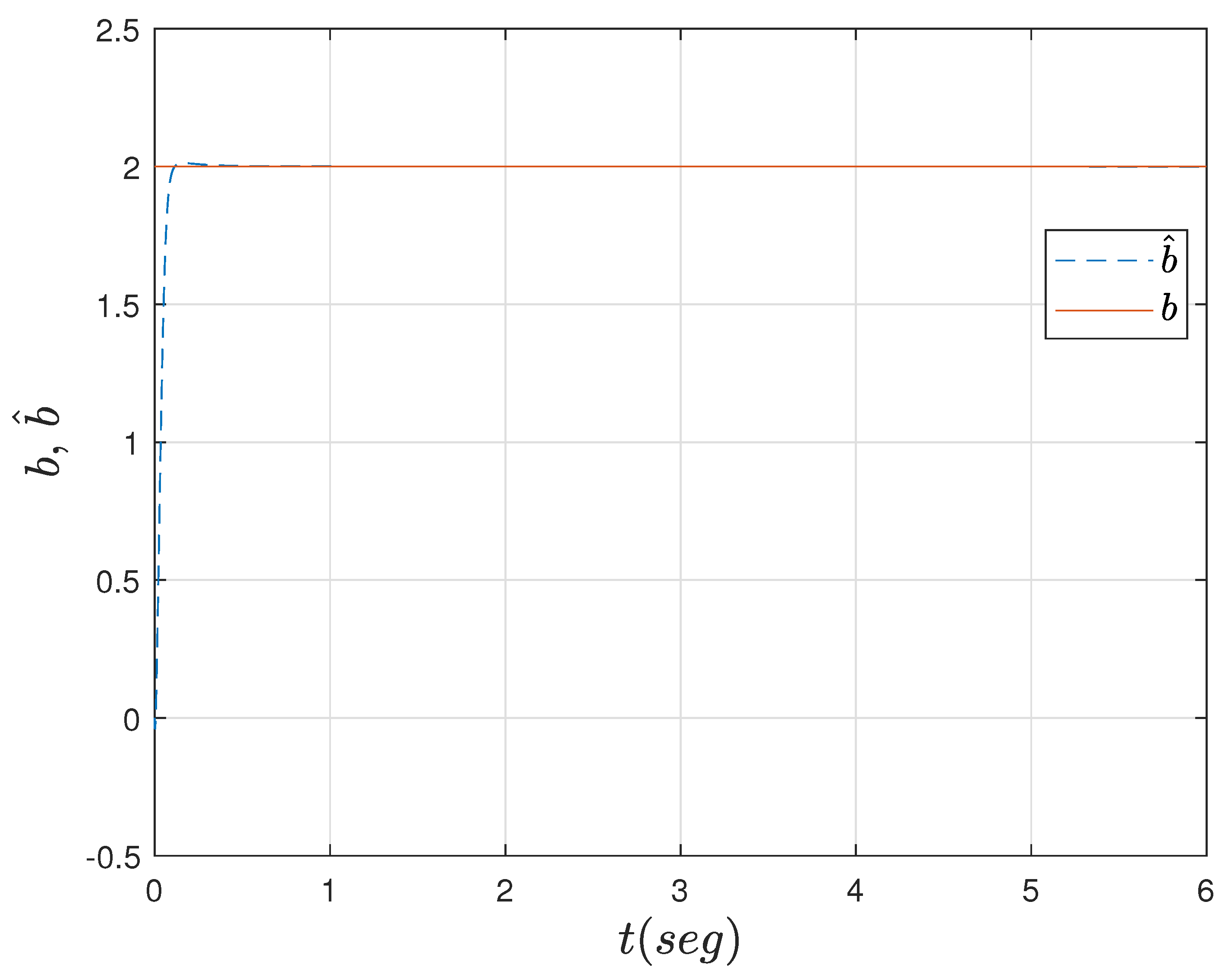
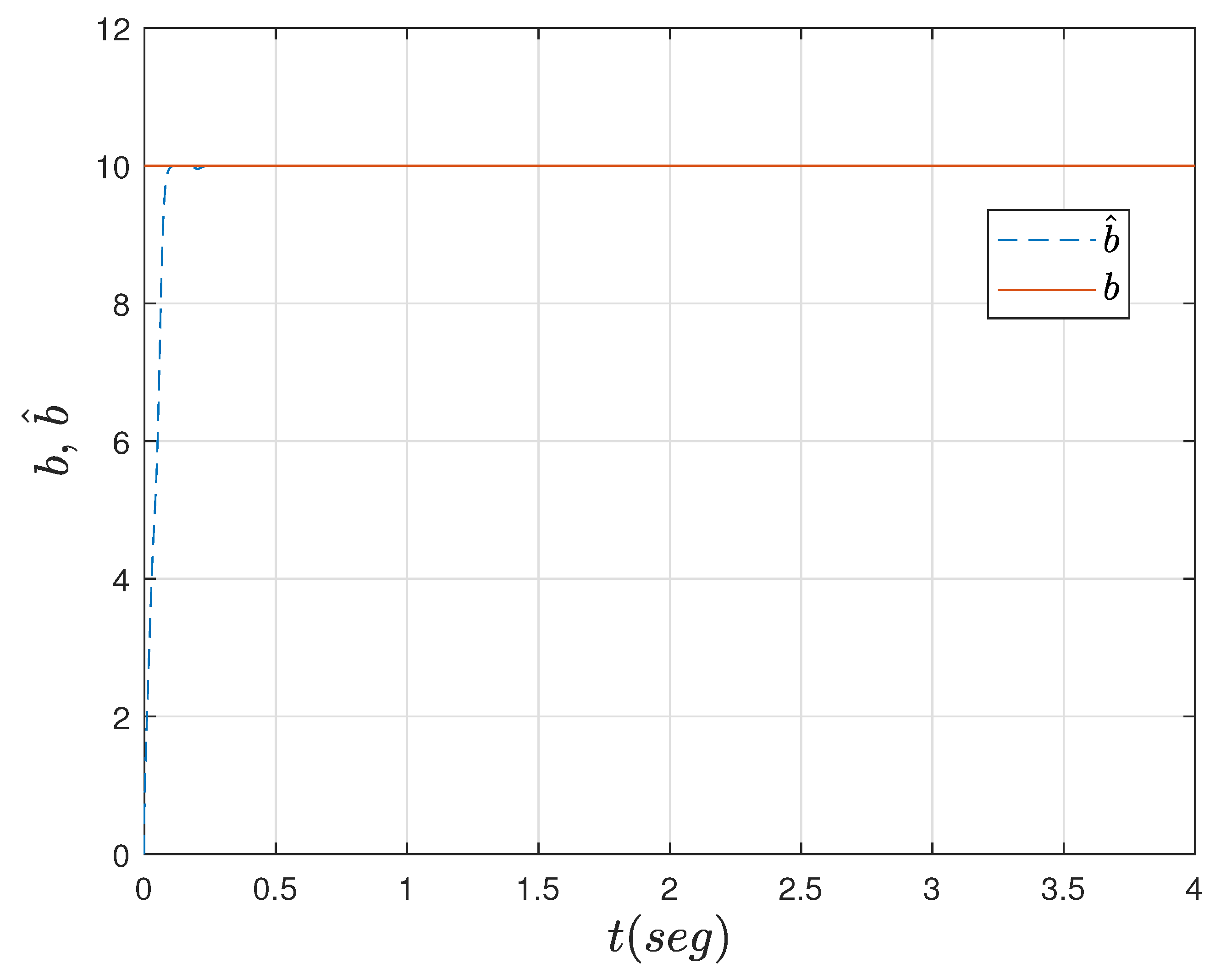
In the manner described above, it has been proved that the system (20)–(22) effectively estimates $\widehat{b}$ and $\widehat{\lambda }$ which converge to the true parameters b and $\lambda$ via adaptive laws (39)–(40), allowing for the dynamics of the system (20)–(22) also converge with that from (13)–(15). Then, the following lemma can be stated.

Lemma 1.

The identifier (20)–(22) with update laws (39)–(40) guarantees

$$\begin{array}{ccc}\hfill \parallel e\left(t\right)\parallel & \in & {\mathcal{L}}_{\infty }\cap {\mathcal{L}}_2,\hfill \end{array}$$

(44)

$$\begin{array}{ccc}\hfill \parallel e_x\left(t\right)\parallel ,\parallel u_x\left(t\right)\parallel \parallel e\left(t\right)\parallel & \in & {\mathcal{L}}_2,\hfill \end{array}$$

(45)

$$\begin{array}{ccc}\hfill \tilde{b}\left(t\right),\tilde{\lambda }\left(t\right)& \in & {\mathcal{L}}_{\infty },\hfill \end{array}$$

(46)

$$\begin{array}{ccc}\hfill \dot{\widehat{b}}\left(t\right),\dot{\widehat{\lambda }}\left(t\right)& \in & {\mathcal{L}}_2.\hfill \end{array}$$

(47)

From Lemma 1, although the stability of the identifier has been proven, the proof for closed-loop stability of the whole adaptive boundary control scheme designed here can be carried out along the same lines as in [24].

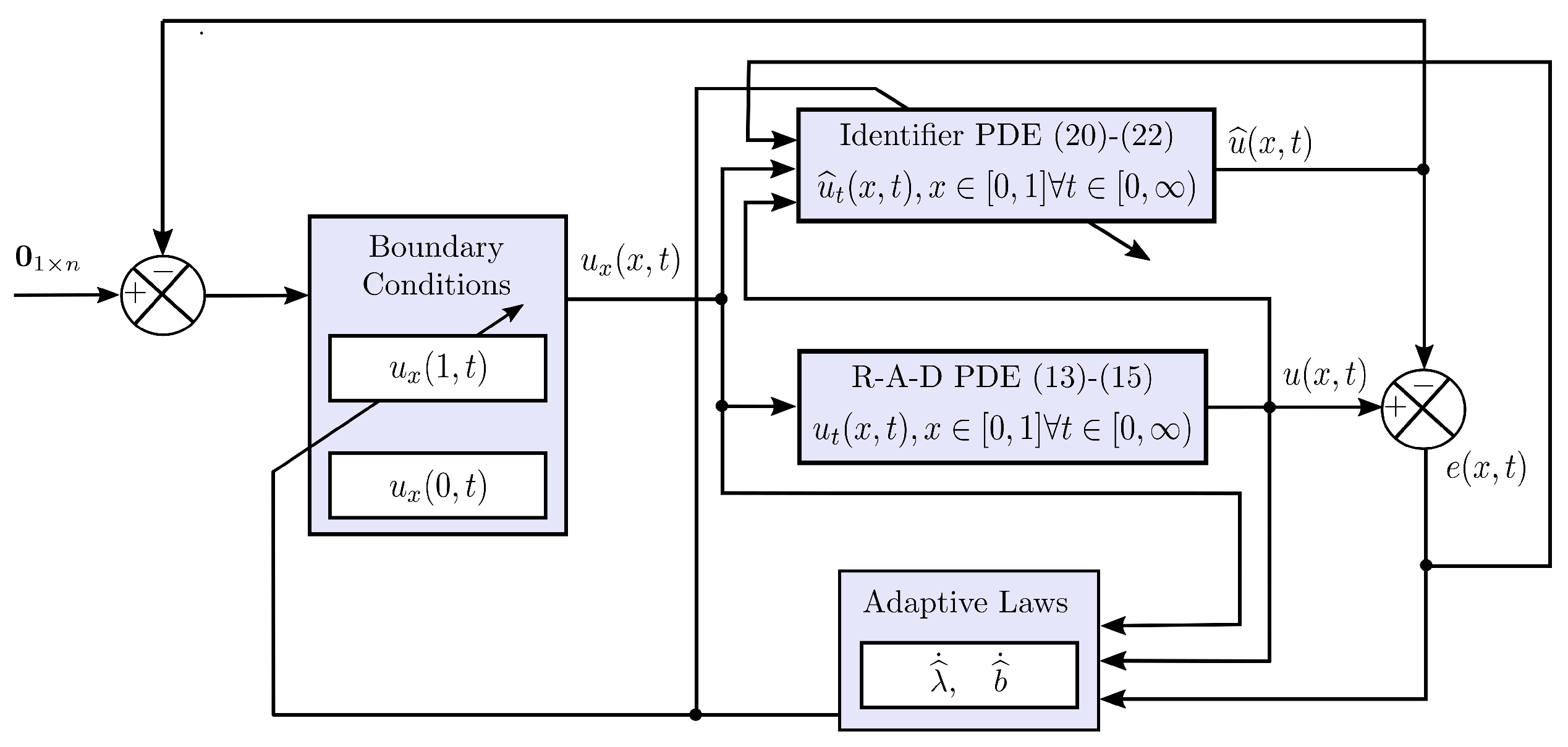
In Figure 1, a block diagram is shown to illustrate the adaptive control scheme for the R–A–D PDE system (13)–(15).

7. Simulation Results

In this section, we discuss the simulation results from the dynamics in the closed loop of the adaptive Neumann stabilizing controller. The main objective is to show the convergence to zero for the estimation error (25) as a function of time and that the estimated parameters $\widehat{b}$ and $\widehat{\lambda }$ converge to their true values as time progresses. The simulation is set to $b=2$ and $\lambda =12$ along with initial condition $u_0\left(x\right)=10sin\left(\pi x\right)$. A built-in function in MATLAB with a previous finite discretization in space process to solve a resulting $2\times 2$ parabolic PDE system, consisting of the R–A–D PDE system (13)–(15) and identifier PDE (20)–(22), is implemented. Figure 2 shows the dynamics of the R–A–D PDE system with adaptive Neumann control at the boundary while Figure 3 shows the progression in time of the identifier PDE. The dynamics from the identifier PDE are very similar to that from the R–A–D PDE system. Figure 4 clearly shows how the estimation error (25) converges to zero almost immediately after starting the process. In Figure 5, we can see the effort of the control signal (24), where the parametric estimates $\widehat{b}$ and $\widehat{\lambda }$ actively affect its behavior as they are computed at each time interval. Figure 6 and Figure 7 show the progression of convergence over time of the estimated parameters $\widehat{\lambda }$ and $\widehat{b}$ versus their true values, respectively. The performance of the adaptive Neumann stabilizing control scheme but for parameters set to $b=10$ and $\lambda =30$ and initial condition $u_0\left(x\right)=5(1-2sin(3\pi x/2))$ is shown from Figure 8, Figure 9, Figure 10, Figure 11, Figure 12 and Figure 13.

8. Conclusions

In this work, an adaptive Neumann stabilizing controller is designed to a certain class of an R–A–D PDE system under the assumption of unknown constant parameters to the reaction and advection terms along with combined boundary conditions of both Robin and Neumann type. The performance of the adaptive boundary controller is evaluated via numerical simulation. Simulation results from the convergence to zero for the estimation error as well as the convergence of the parametric estimates to their true (assumed as unknowns but constant) values show that the backstepping-based adaptive boundary control scheme, particularly the certainty equivalence design with passive identifier, also works well with this certain class of PDE system. As future work, the design of an adaptive Neumann stabilizing controller could be explored to try with boundary control of coupled R–A–D PDE systems with spatially-varying coefficients, or having the same diffusivity parameter, but with both Robin and Neumann boundary conditions or to extend our proposal to the case of distributed actuation and unknown input delay.