Abstract
Multi-class classification in imbalanced datasets is a challenging problem. In these cases, common validation metrics (such as accuracy or recall) are often not suitable. In many of these problems, often real-world problems related to health, some classification errors may be tolerated, whereas others are to be avoided completely. Therefore, a cost-sensitive variable selection procedure for building a Bayesian network classifier is proposed. In it, a flexible validation metric (cost/loss function) encoding the impact of the different classification errors is employed. Thus, the model is learned to optimize the a priori specified cost function. The proposed approach was applied to forecasting an air quality index using current levels of air pollutants and climatic variables from a highly imbalanced dataset. For this problem, the method yielded better results than other standard validation metrics in the less frequent class states. The possibility of fine-tuning the objective validation function can improve the prediction quality in imbalanced data or when asymmetric misclassification costs have to be considered.
1. Introduction
Machine learning methods are pervasive nowadays, and classification is one of the main problems within this field [1,2]. Classification consists of predicting the value or state of a discrete variable of interest, called the class, given the values of other variables, called the predictive or feature variables. Multi-class classification [3,4] is a specific classification problem, in which the class variable has more than two possible values, as opposed to the usual binary classification. Some authors propose the adaptation of binary classification methods to deal with multi-class data [5,6,7], but these techniques often present inconveniences.
In real-world datasets, the distribution of the class variable is usually far from being uniform, with some classes being much more frequent than others. This kind of data is called imbalanced [8,9]. As the rare classes have few cases to learn from, standard classifiers tend to learn the rules to classify the common classes and ignore the rare ones. Consequently, rare classes are usually misclassified. In some applications, such as cancer or fraud detection, the main concern is precisely the identification of infrequent cases. This is especially problematic in multi-class schemes [10,11].
Many solutions have been proposed to tackle binary classification for imbalanced data [8,9,12], including balancing the classes by means of resampling (e.g., oversampling of the rare class or undersampling of the common class [13]), or improving the recognition of the underrepresented class. Some solutions applied to binary imbalanced data are not practical for multi-class imbalanced data [14,15], especially resampling methods, due to the increase in complexity. In this case, algorithm level approaches, which try to bias the classification learning towards the rare classes, are more commonly applied.
Variable or feature selection [16,17,18,19] can play a crucial role when facing imbalanced data [20]. An excessive number of variables may decrease both the generalization of the model by over-fitting and its performance by introducing noise. Therefore, variable selection methods aim at choosing the set of variables that better discriminates between the classes of the target variable, i.e., irrelevant or redundant variables are usually discarded in order to improve the performance of the model.
Bayesian networks (BNs) [21,22] have been employed successfully for classification purposes [23] in many applications [24,25,26,27,28,29], including multi-class tasks [30]. Roughly speaking, BNs are compact representations of the joint probability distribution over a set of variables, whose independence relationships are encoded by a directed acyclic graph [21]. In the context of classification, the use of fixed or restricted structures is widespread since they allow the reduction of the number of parameters to be estimated from data while maintaining the accuracy of the model [24].
We propose a cost-sensitive [31,32,33] variable selection method for multi-class imbalanced data [34], in the sense that the validation metric takes into account the different impact of each error type in the classification errors. Thus, one can specify a priori a cost or loss function encoding the problem-specific aspects (i.e., the cost/loss of each kind of misclassification). Then, using a variable selection algorithm, this cost-based metric is optimized, and the best-fitting variables are selected. Our main contribution is the introduction of a validation metric that generalizes the standard classification metrics (i.e., accuracy, precision, and recall) by using custom cost matrices that allow different misclassification penalties. In order to test the proposed approach, we apply it to the problem of forecasting the next-hour air quality from air pollutants and climate data, using a highly imbalanced real dataset. This dataset was chosen as a case study due to its severe imbalance and the different impact of each misclassification type.
Many predictive models have been proposed for air quality forecasting in the last few years using machine-learning [35], most of them employing neural networks or other deep learning techniques [36,37]. In [36], different neural network structures were tested for both short-term and long-term predictions. In [37], deep neural networks are also used but including spatial and geographical information. Other works, like [38], have proposed several regularization techniques to increase the model performance and to reduce over-fitting.
Bayesian networks (BNs) and Bayesian methods have also been used for air pollution prediction [39,40,41,42]. In [39], BNs were successfully used for predicting ozone levels through structural learning. Other more recent works have employed BNs for predicting the air quality with a fixed set of predictors in Shanghai (China) [40] and in Genoa (Italy) [41]. In the former, a general structure is compared to other models, whereas, in the latter, an expert-elicited model is compared to an automatically built structure. However, these two works look rather elementary, and few details on the methodology and experimental set-ups were given. A more exhaustive list of machine-learning contributions to forecasting air pollutants or air quality can be found in [38,42].
Regarding the air quality prediction problem, we propose to use the aforementioned methodology to improve the classification rate on the infrequent class states (which normally correspond to harmful pollution levels), which consists of using a variable selection procedure and a more general validation metric that allows custom misclassification penalizations.
The structure of the rest of the paper is as follows. In Section 2, we give a brief overview of Bayesian networks, a description of a parsimonious variable selection procedure, and we describe the multi-class classification problem and discuss how to validate a multi-class model. Then, still in Section 2, we introduce the problem of forecasting an air quality index and propose custom cost functions for it. In Section 3, we present and describe the experimental results of the proposed approach, testing it with air quality data. Finally, in Section 4, we discuss the results and comment on their main implications.
2. Methodology
2.1. Bayesian Networks
A Bayesian network is a compact representation of the joint probability distribution over a set of variables , whose independence relations are encoded by the structure of an underlying directed acyclic graph (DAG) [21,22]. Briefly speaking, a BN is defined as a pair , where G is a DAG and P is a set of conditional probability distributions (CPDs). G is composed of nodes that represent random variables (), and links between pairs of nodes representing statistical dependence. Each node has an associated probability distribution , where denotes the parents of in the DAG G. Attending to the factorization encoded in the DAG, the joint probability distribution over all the variables in the network is defined as the product of the CPDs attached to each node, so that
where represents the domain or set of all possible values of the variable .
Figure 1 shows an example of a Bayesian network, whose joint distribution for variables can be factorized as
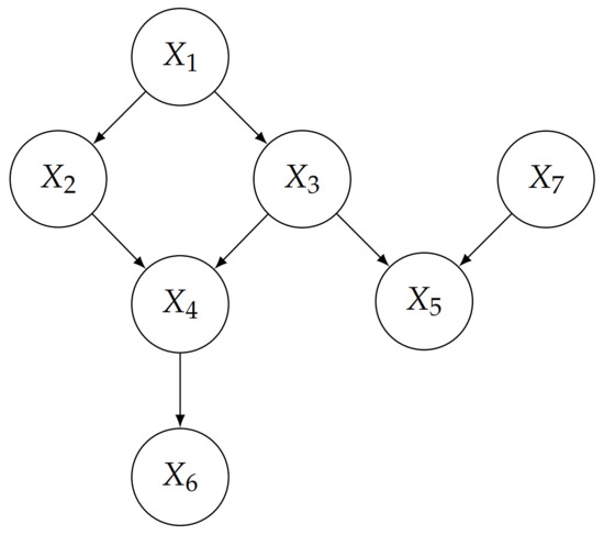
Figure 1.
An example of a Bayesian network.
When a BN contains both discrete and continuous nodes, it is called a hybrid BN. A hybrid BN classifier is a BN that contains a discrete variable of interest C and a set of predictive (continuous or discrete) variables . The goal of such a classifier is to determine the probability that an object with observed features belongs to each class , and to return the most likely one [23]:
A number of restricted DAGs have been proposed to solve regression tasks, aiming at reducing the number of parameters to be estimated from data while maintaining the accuracy of the model [23,24]. The simplest case is the naive Bayes (NB), a fixed structure whose class variable C is the parent of all remaining explanatory variables , i.e., links point from C to each . In other words, the predictors are considered independent of each other given C. The strong independence assumption is compensated by the reduction in the number of parameters to be estimated from data since the posterior probability distribution over the class variable C is computed as follows:
There exist other restricted and more elaborated structures that relax the independence assumption, for instance, k-dependence Bayesian classifiers (kDB), which allow that each feature has up to k more parents besides the class variable. The naive Bayes is a special case of kBDs, where [23]. Learning the structure of restricted models can be done from data by means of constraint-based techniques or greedy search techniques [23,43]. These approaches can also be used to learn unrestricted structures, i.e., those that do not distinguish a class variable. However, these techniques are often computationally expensive and harder to implement. Moreover, the naive Bayes model has repeatedly shown excellent performance in classification problems.
In this study, a conditional linear Gaussian (CLG) Bayesian network with naive Bayes structure is considered. More precisely, the class C is a multinomial variable with four states, and the remaining nodes are continuous variables. Even though exact inference is feasible in this case, approximate inference is easier to implement and to generalize to more complex network structures. Approximate inference includes algorithms such as evidence or likelihood weighting [44], importance sampling [45], and other techniques [22,43]. The R package bnlearn [46], which includes an implementation of the likelihood weighting algorithm, was used to build the hybrid BN classifier.
2.2. Variable Selection
A variable selection process was carried out using an incremental wrapper sequential subset with replacement method [47]. Let C be the class variable, i.e., the variable we are interested in classifying, and the set of predictive variables of C. Let be the set of variables included in the classification model . Firstly, we need to determine an order for the predictive variables . Let be the ordered set of the predictive variables.
To initialize the algorithm, the first variable in () and the class C are included in . Then, the variables in are used to build a classification model, , and a measure of predictive performance, V, is computed using the k-fold cross-validation technique [48]. This technique splits the complete dataset into k subsets, with k-1 being used to learn the model (train set) and the other to compute the predictive performance (test set). The splits are obtained randomly and maintaining the proportions of the different values of the class variable. This method is repeated k times so that a new train and test sets are used each time. The average of the k performance measures (V), giving an estimate of the out-of-sample loss. In our experiments, a k-value of 10 was applied.
After the initial model is obtained, the next variable in () can either be added to , replace a predictive variable in or not being included in . The criteria to decide the path of the variables in depends on the predictive performance of the new classifier, . More precisely, each variable in always takes the following steps (not necessarily in this order):
- it replaces the predictive variables in , one by one, and the predictive performance, , of the new classifier, , is computed. If the predictive performance of is higher, i.e., , the new variable replaces and the predictive performance () is set as the current one (V);
- it is inserted in and the predictive performance of , , is computed. If , is kept in and V = .
These steps are repeated for all the variables in and the loop starts over as long as the model’s performance improves. The details for the variable selection method carried out are shown in Algorithm 1.
The predictive performance of model can be measured with any metric of interest, such as the global accuracy, the recall or precision of a class, among others. Section 2.3 further discusses the validation metrics used in this work.
| Algorithm 1: Incremental Wrapper Sequential Subset with Replacement (IWSR) |
 |
2.3. Multi-Class Classification
In binary classification, the most common validation metrics are accuracy, precision, and recall. A single metric among these can be rather informative, depending on the specific problem. However, in highly imbalanced datasets, the accuracy may not be reliable. Moreover, in problems where one wants to keep the false-negative rate low, obtaining a high value of the recall rather than the accuracy or the precision is preferable.
Multi-class classification models are challenging to validate. Several strategies have been proposed to reduce multi-class classification to binary classification, such as one-versus-all and all-versus-all schemes [15,49]. However, this approach may generate a large number of models and metrics, and it is preferable to use purely multi-class classifiers.
In a multi-class problem, it is often impossible to compare models with a single metric, or even with a few of them. In particular, in a multi-class scheme, there are not single values for precision and recall, but there are different values for each class variable state. The validation or the selection of a model will rely critically on the chosen metrics.
Classification results can be gathered in what is called the confusion matrix, either represented as a table (Table 1, left) or purely as a matrix: , where we assume r class values or states. The value , in row i and column j, stands for the number of observations whose class value is and were classified as being of class . From these values, we can compute , the absolute frequency of class value i, as , and the total number of observations, . The sum of the main diagonal, , yields the total number of correct classifications, whereas values out of that diagonal, with , represent misclassifications. From the confusion matrix, the accuracy (fraction of correct predictions) is computed simply as . The recall and precision for class k can be calculated as:
whose denominators are respectively the sums of elements in row k and column k, and the common numerator is the number of correctly classified observations in class k.

Table 1.
Confusion matrix (left) and loss matrix (right) for multiclass classification with r states.
All these metrics are symmetric, in the sense that the importance of every classification error is the same. Therefore, there are many problems where these standard metrics are not suitable, due to imbalance in the data or the different cost of classification errors (i.e., misclassifications for some class values have a heavier impact than for other class states). These problems typically arise in diagnostic or health problems, in which it is critical to have a low proportion of false negatives, and the impact of having some false positives is admissible. In these situations, asymmetric costs should be employed to measure the performance of a model.
To overcome these inconveniences, we propose an extension of the metrics above that generalizes them and permits establishing different weights for every possible classification. We define , which is a weight for the classification of class state i as j. These will be a cost or loss in case of failure () but a benefit or reward in the case of success (). These weights can be collected in what we call a loss matrix, , even though values in the main diagonal actually correspond to rewards (see Table 1, right). Absolute cost/reward values in this matrix are not relevant, as long as the ratios between different types of errors are kept.
Using the loss matrix , and the confusion matrix introduced above, we define the validation metric V, which depends on both, as:
where the numerator stands for the weighted number of successes and the denominator is the total weighted number of classifications (both successes and failures). This definition of validation metric V is motivated by two aspects: it is a generalization of the usual metrics (accuracy, recall, precision), and it is bounded between 0 and 1, where 1 corresponds to a perfect classification. For instance, if we set to be a matrix full of ones, becomes the usual accuracy. If is a matrix full of zeros but with ones in the row (resp. column) k (see Equation (3) below), then yields the usual recall (resp. precision) for class k. For instance, to recover the precision for class state 1, , and the recall for class state 2, , we can compute and respectively, with the following loss matrices:
Another metric that has been proposed for multi-class classification problems is the geometric mean of the recalls () [50] of each class value (see Equation (4)). Due to the nature of the geometric mean, this metric will try to maximize, simultaneously and with certain homogeneity, all the recall values:
2.4. Forecasting Air Quality Index
To check the proposed approach for cost-sensitive variable selection in multi-class imbalanced data, Algorithm 1 was tested with different objective functions in the problem of forecasting the air quality index (NAQI) one time-step ahead. Several alternatives were employed and analyzed, depending on the objective metric to be optimized in the variable selection process. The six objective functions were: accuracy (), recall for state (), recall for state (), geometric mean of the recalls (), and the two custom cost functions, and , defined in Section 2.4.3.
2.4.1. The NAQI Air Quality Index
In order to establish air quality levels, we use the definition of the National Air Quality Index (NAQI) from Spain, according to the official Spanish methodology [51]. This index comprises the values of five key air pollutants: , , , , and , and the index category is assigned based on the worst level among the pollutants. The explanation of each pollutant can be found in Table 2. For and , the hourly average levels are used in NAQI. For , , and , the index uses the moving average of the values among the last 8, 24, and 24 h, respectively. We will denote these moving averages as , , and , and they will also be used as predictive variables later. There are six possible labels for the NAQI, which, ordered by increasing pollution, are defined in Spanish as: “buena” (good), “razonablemente buena” (fair), “regular” (moderate), “desfavorable” (poor), “muy desfavorable” (very poor), and “extremadamente desfavorable” (extremely poor). Further details can be found in [51].
Table 2.
Description of the predictive variables and their percentage of missing values in the original dataset.
2.4.2. Data Source and Analysis
Three yearly datasets containing a number of relevant pollutants and climatic variables measured hourly were acquired from www.gijon.es/es/datos. These datasets originate from Gijón (Asturias), a city in northern Spain, and covers the period from 2017 to 2019.
The merged dataset contained missing values, which were imputed using the R package missForest. On the other hand, the first 23 h were removed since the computation of the moving averages leads to data loss. Moreover, the last observation (i.e., the last hour of the last day) was also removed since no data were available for the next hours. Table 2 shows the description of the predictive variables considered, as well as their percentage of missing values in the original dataset. The completed dataset was used to compute the air quality index (NAQI), described above. Since our goal is to predict the NAQI value one hour ahead, we shifted this variable one time step behind. The NAQI variable, i.e., the class in this case study, is a highly imbalanced multinomial variable with four states. Table 3 shows the relative frequency of each category of the class variable.
Table 3.
Relative frequency (%) of each category of the class variable (NAQI) and sample sizes for the complete, train, and test datasets.
For an adequate validation of the models, the dataset was split into training and test datasets. The train set corresponds to years 2017 and 2018 ( of the total observations), whereas data in the test set correspond to 2019 (). These two datasets contain a similar proportion of the class categories (see Table 3). The train set was used for running the cost-sensitive variable selection procedure (Algorithm 1) to optimize different cost metrics. The test set was employed exclusively for a final independent validation of the models learned with the training dataset.
2.4.3. Custom Cost Functions for the Air Quality Problem
In the problem of forecasting the air quality index, the correct identification of the worst levels is crucial. In the dataset analyzed, these are states 3 and 4, which correspond to levels “Moderate” (the second most critical state to identify in this dataset) and “Poor” (the most critical state), respectively, and also are, by far, the two less frequent classes in the dataset (see Table 3). With the aim of improving the predictions on class states 3 and 4, two custom cost functions were proposed as follows.
The first one was given by an explicit formula taking into account the relative frequencies of the class states so that the most frequent classes are less relevant in the validation metric. To do that, we computed the costs: , where stands for the absolute frequency of class state i (; their values can be deduced from Table 3). We will refer to this cost function as . With this definition, if a class state is much less frequent than , the cost of misclassifying the class state i as j is very high. On the contrary, if is much more frequent than , the misclassification of i as j is not severely penalized, as the cost is around 1. For this specific problem, the resulting loss matrix is displayed in Table 4 (left). This kind of cost-sensitive metric is general and may be useful for other imbalanced problems as well, in which asymmetrical costs make sense.
Table 4.
The two custom loss matrices, (left) and (right), used for variable selection in the problem of forecasting the next-hour national air quality index (NAQI) value.
The second custom loss function was set manually with the aim of improving the predictions, especially the recalls on class states 3 and 4, which are the two less frequent values and correspond to the two worst air quality levels. With that goal, we defined the loss function given by the asymmetric loss matrix given in Table 4 (right). We will refer to this cost function as .
3. Results
The proposed approach for cost-sensitive variable selection in multi-class imbalanced data was tested using six objective functions: accuracy (), recall for state (), recall for state (), geometric mean of the recalls (), and the two custom cost functions and defined previously. For each objective function, 10 independent runs were executed, and, for each run, the variable selection algorithm in Algorithm 1 was employed for optimizing the objective function across the training dataset. After finishing, a set of selected variables was obtained for each objective function (see Table 5). A number between five and eight variables were selected for each objective function, with and being the ones selecting fewer variables, and and the ones selecting more variables. The most frequently selected variable (selected by all models) was , followed by , , and (selected five out of six times).
Table 5.
Selected variables depending on the optimization objective function.
Figure 2 shows the distribution of the most frequently selected variables for each value of the air quality index (those selected in more than one model). For some predictive variables, differences among their distributions are noticeable (, , , , ). However, for other predictors (, , ), the distributions are rather overlapped, which might make the discrimination among the class values more difficult and, therefore, yield a worse classification performance. Nevertheless, even if some of these variables do not individually discriminate between the class states, they still help improve the classification performance when combined with others.
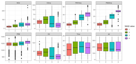
Figure 2.
Box-plots of some of the predictive variables for each value of the air quality index.
After the variable selection process, the models were fit again using the training set, restricted to the selected variables, and their performances were analyzed using the test set, in order to carry out an independent validation. The accuracy of each model over the test set is reported in Table 6, and the recall and precision for each class state and each model are reported in Table 7. The best accuracy, recalls, and precisions for class states 3 and 4 are highlighted in boldface. Figure 3 shows the pair precision–recall for each class state and optimized objective function, plotted from the figures in Table 7. Note that the higher and more to the right a point is, the better.
Table 6.
Accuracy over the test set for each objective metric. The best value is highlighted in boldface.
Table 7.
Recall and precision over the test set for each validation metric and for each class state. The best values for class states 3 and 4 are highlighted in boldface.
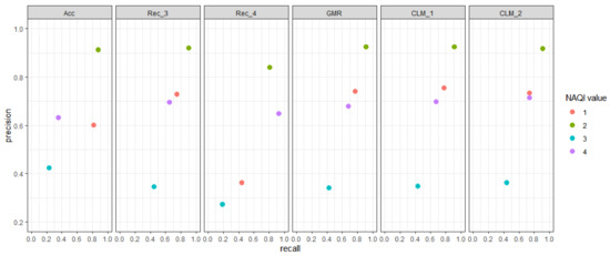
Figure 3.
Results of precision–recall pairs for each class state and each optimized objective function (by columns).
The objective metrics show an accuracy value between ≈0.72 and ≈0.87, with being the most accurate, closely followed by , and being the least accurate, followed by (Table 6). Note that the model with objective function is the second-worst model in terms of accuracy, even though it was trained to maximize this measure.
Regarding recall and precision (Table 7), no objective function outperforms the others in all class states. Class state 1 has a recall around in all objective metrics, except for , which obtains a value of ≈0.44. In terms of precision, the pattern is similar, obtains a lower value in comparison with the others. Regarding the recall and precision of class 2, most objective metrics obtain a value of around , except for , which obtains lower values. Class state 3 is the most difficult to classify, as all objective metrics get recall values up to (), and precision values up to (). Finally, gets the highest recall for class 4 () and second-lowest precision (), with getting the highest precision () and second-highest recall ().
4. Discussion
The problem of multi-class classification presents some characteristics that make it much more complex than the binary case [15]. One of the most relevant aspects is the imbalance, or very marked non-uniformity, in the distribution of the class values [8]. In these cases, the metrics usually used to measure the predictive quality of the models, such as accuracy, precision, or recall, may not be suitable for the model validation [10,11].
In addition, in some of these problems, the impact of a classification error varies dramatically depending on the actual class and the predicted class. For example, this happens in real-world models related to the diagnosis of diseases, public health issues, the occurrence of natural disasters, or other similar situations. Ideally, it would be desirable that there were no classification errors. However, if this is not possible, one strategy is to be more conservative in the predictions, so that the most severe cases are detected correctly, even if this means that a higher number of less serious class states are misclassified.
In this work, we propose an approach for dealing with multi-class imbalanced datasets, employing a flexible validation metric that encodes the different impacts of classification errors. These kinds of techniques are sometimes referred to as cost-sensitive [32,33]. To build the predictive model or classifier, we use a variable selection algorithm [47] that parsimoniously adds or removes variables to increase the model performance. This performance is measured according to a specific cost or loss function in order to take into account the different types of classification errors adequately.
As proof of concept, the proposed methodology has been applied to predict an air quality index (NAQI [51]) using current levels of air pollutants and climatic variables. The incorrect identification of poor air quality events may jeopardize sensitive individuals (children, seniors, lung, or heart diseases) or even healthy people, worsening their symptoms and quality of life [52,53]. In these episodes, the authorities usually recommend to avoid or reduce outdoors activities [54]. Therefore, it is desirable to be able to reliably identify these events in advance.
In the analyzed air quality problem, the results show some interesting facts. The model built to optimize the accuracy over the training set is the second-worst in accuracy over the test set. This suggests overfitting in that model and remarks the need for independent validation of the model results. By contrast, the methods and that were optimized for recall over the training set on class states 3 and 4, respectively, keep leading these metrics in the test set as well; however, they reduce the recall of other class states, especially .
If we consider class states 3 and 4 at the same time, and are the two best alternatives, closely followed by , with being the best-performing if we focus on state 4. According to the results, seems to yield the most balanced results on the minority class states, which are also the most relevant to predict in this problem. Therefore, the custom loss metrics were capable of improving the prediction quality and a better forecasting of high pollution episodes.
The proposed cost-sensitive variable selection method can be employed not only with a Bayesian network classifier, but with any other classification technique (e.g., CNNs, SVMs, random forests, etc.). This approach also allows the use of probabilistic loss functions (e.g., log-likelihood, or similar). In that case, the model would necessarily have to be probabilistic too, which is a natural property of the Bayesian networks.
Concerning the air quality problem, the use of Bayesian networks is scarce in the literature, and the works are often rudimentary. Unlike other related papers [40,41,42], the method we propose allows an optimal selection of the predictive variables. It also performs a more adequate evaluation of the models for this highly imbalanced multi-class problem using custom loss metrics, which can improve the prediction quality over the infrequent class states. As opposed to [42], we use a purely multi-class model, avoiding the need to establish thresholds for discriminating different class levels. In this work, we have chosen the naive Bayes structure for the classifier, since it is flexible enough and cost-effective [24]. Nevertheless, a more complex Bayesian network structure could yield better classification results for the air quality prediction, as [40] suggests. However, the computational complexity of the variable selection algorithm could increase significantly if it is combined with a structural learning procedure.
A relevant part of our approach is the choice of the custom loss matrix to be used in Equation (2). In [42], they propose the ranked probability score (RPS) metric, whose misclassification weights are the distances between the class values. However, the use of an adjustable loss matrix permits a better fit to a specific problem, which is essential in the context of imbalanced data. The costs in should reflect the nature of the problem and the impact of the classification errors in each case. Although there is not a general recipe, the costs should normally be non-negative, and their values should increase with if the class variable is ordinal, or reflect the relative frequencies of the class states for heavily imbalanced data, in order to favor the infrequent values (see Section 2.4.3).
To summarize, we have presented a possible generalization of the usual validation metrics for classification, which can codify the cost or reward of the different classification outcomes. Using it, a variable selection algorithm was able to select the best-performing variables for the less frequent class states in a highly imbalanced dataset. The selected variables improved the results over the infrequent class values in an independent validation. The possibility of fine-tuning the objective validation function can improve the prediction quality in imbalanced data or when asymmetric misclassification costs have to be taken into account.
Author Contributions
The two authors contributed equally to all aspects of research. All authors have read and agreed to the published version of the manuscript.
Funding
This research received no external funding.
Institutional Review Board Statement
Not applicable.
Informed Consent Statement
Not applicable.
Data Availability Statement
The data used in this work can be found at www.gijon.es/es/datos.
Acknowledgments
D.R.-L. thanks the support from the Center for Development and Transfer of Mathematical Research to Industry CDTIME (University of Almería), from the research group FQM-229 (Junta de Andalucía), and from the ‘Campus de Excelencia Internacional del Mar’ CEIMAR (University of Almería).
Conflicts of Interest
The authors declare no conflict of interest.
Abbreviations
The following abbreviations are used in this manuscript:
| DAG | Directed acyclic graph |
| BN(s) | Bayesian network(s) |
| CLG | Conditional linear Gaussian |
| CPD | Conditional probability distributions |
| CM | Confusion matrix |
| LM | Loss (cost) matrix |
| Accuracy | |
| Recall for class state k | |
| Precision for class state k | |
| Geometric mean of the recalls | |
| Custom loss matrix k () | |
| Obs. | Observed values |
| Pred. | Predicted values |
| NAQI | National Air Quality Index (Spanish official air quality index) |
References
- Jordan, M.I.; Mitchell, T.M. Machine learning: Trends, perspectives, and prospects. Science 2015, 349, 255–260. [Google Scholar] [CrossRef] [PubMed]
- Murphy, K. Machine Learning: A Probabilistic Perspective; Adaptive Computation and Machine Learning; MIT Press: Cambridge, MA, USA, 2012. [Google Scholar]
- Rau, A.; Nadal, J.P. A model for a multi-class classification machine. Phys. A Stat. Mech. Appl. 1992, 185, 428–432. [Google Scholar] [CrossRef]
- Chaitra, P.; Kumar, D.R.S. A review of multi-class classification algorithms. Int. J. Pure Appl. Math. 2018, 118, 17–26. [Google Scholar]
- Li, T.; Zhu, S.; Ogihara, M. Using discriminant analysis for multi-class classification: An experimental investigation. Knowl. Inf. Syst. 2006, 10, 453–472. [Google Scholar] [CrossRef]
- Kang, S.; Cho, S.; Kang, P. Constructing a multi-class classifier using one-against-one approach with different binary classifiers. Neurocomputing 2015, 149, 677–682. [Google Scholar] [CrossRef]
- Yang, X.; Yu, Q.; He, L.; Guo, T. The one-against-all partition based binary tree support vector machine algorithms for multi-class classification. Neurocomputing 2013, 113, 1–7. [Google Scholar] [CrossRef]
- Chawla, N. Data Mining for Imbalanced Datasets: An Overview. In Data Mining and Knowledge Discovery Handbook; Maimon, O., Rokach, L., Eds.; Springer: New York, NY, USA, 2005; pp. 853–867. [Google Scholar] [CrossRef]
- Shakeel, F.; Sabhitha, A.S.; Sharma, S. Exploratory review on class imbalance problem: An overview. In Proceedings of the 8th International Conference on Computing, Communication and Networking Technologies (ICCCNT), Delhi, India, 3–5 July 2017; pp. 1–8. [Google Scholar] [CrossRef]
- Wang, S.; Yao, X. Multiclass imbalance problems: Analysis and potential solutions. IEEE Trans. Syst. Man Cybern. Part B 2012, 42, 1119–1130. [Google Scholar] [CrossRef]
- Ortigosa-Hernández, J.; Inza, I.; Lozano, J.A. Measuring the class-imbalance extent of multi-class problems. Pattern Recognit. Lett. 2017, 98, 32–38. [Google Scholar] [CrossRef]
- Norinder, U.; Boyer, S. Binary classification of imbalanced datasets using conformal prediction. J. Mol. Graph. Model. 2017, 72, 256–265. [Google Scholar] [CrossRef]
- Estabrooks, A.; Jo, T.; Japkowicz, N. A multiple resampling method for learning from imbalanced data sets. Comput. Intell. 2004, 20, 18–36. [Google Scholar] [CrossRef]
- Sun, Y.; Wong, A.K.; Kamel, M.S. Classification of imbalanced data: A review. Int. J. Pattern Recognit. Artif. Intell. 2009, 23, 687–719. [Google Scholar] [CrossRef]
- Sahare, M.; Gupta, H. A review of multi-class classification for imbalanced data. Int. J. Adv. Comput. Res. 2012, 2, 160. [Google Scholar]
- Bell, D.A.; Wang, H. A formalism for relevance and its application in feature subset selection. Mach. Learn. 2000, 41, 175–195. [Google Scholar] [CrossRef]
- Inza, I.; Larrañaga, P.; Etxeberria, R.; Sierra, B. Feature subselection by Bayesian networks based optimization. Artif. Intell. 2000, 123, 157–184. [Google Scholar] [CrossRef]
- Mladenic, D. Feature Selection for Dimensionality Reduction. In Subspace, Latent Structure and Feature Selection; Lecture Notes in Computer Science; Springer: Berlin, Germany, 2006; Volume 3940, pp. 84–102. [Google Scholar]
- Vesselinov, V.V.; Alexandrov, B.S.; O’Malley, D. Contaminant source identification using semi-supervised machine learning. J. Contam. Hydrol. 2018, 212, 134–142. [Google Scholar] [CrossRef]
- Fu, G.H.; Xu, F.; Zhang, B.Y.; Yi, L.Z. Stable variable selection of class-imbalanced data with precision–recall criterion. Chemom. Intell. Lab. Syst. 2017, 171, 241–250. [Google Scholar] [CrossRef]
- Pearl, J. Probabilistic Reasoning in Intelligent Systems; Morgan-Kaufmann: San Mateo, CA, USA, 1988. [Google Scholar]
- Korb, K.B.; Nicholson, A.E. Bayesian Artificial Intelligence; CRC Press: Boca Raton, FL, USA, 2010. [Google Scholar]
- Bielza, C.; Larrañaga, P. Discrete Bayesian network classifiers: A survey. ACM Comput. Surv. 2014, 47, 1–43. [Google Scholar] [CrossRef]
- Friedman, N.; Geiger, D.; Goldszmidt, M. Bayesian Network Classifiers. Mach. Learn. 1997, 29, 131–163. [Google Scholar] [CrossRef]
- Mohanty, R.; Ravi, V.; Patra, M. Classification of web services using bayesian network. J. Softw. Eng. Appl. 2012, 5, 291–296. [Google Scholar] [CrossRef]
- Mittal, A.; Cheong, L.H. Addressing the problems of Bayesian network classification of video using high-dimensional features. IEEE Trans. Knowl. Data Eng. 2004, 16, 230–244. [Google Scholar] [CrossRef]
- Kang, Z.; Yang, J.; Zhong, R. A bayesian-network-based classification method integrating airborne lidar data with optical images. IEEE J. Sel. Top. Appl. Earth Obs. Remote Sens. 2016, 10, 1651–1661. [Google Scholar] [CrossRef]
- Castro-Luna, G.M.; Martínez-Finkelshtein, A.; Ramos-López, D. Robust keratoconus detection with Bayesian network classifier for Placido-based corneal indices. Contact Lens Anterior Eye 2020, 43, 366–372. [Google Scholar] [CrossRef]
- Maldonado, A.D.; Aguilera, P.A.; Salmerón, A. Modeling zero-inflated explanatory variables in hybrid Bayesian network classifiers for species occurrence prediction. Environ. Model. Softw. 2016, 82, 31–43. [Google Scholar] [CrossRef]
- Farid, D.M.; Zhang, L.; Rahman, C.M.; Hossain, M.A.; Strachan, R. Hybrid decision tree and naïve Bayes classifiers for multi-class classification tasks. Expert Syst. Appl. 2014, 41, 1937–1946. [Google Scholar] [CrossRef]
- Elkan, C. The foundations of cost-sensitive learning. In Proceedings of the International Joint Conference on Artificial Intelligence, Seattle, WA, USA, 4–10 August 2001; Volume 17, pp. 973–978. [Google Scholar]
- Liu, X.Y.; Zhou, Z.H. The influence of class imbalance on cost-sensitive learning: An empirical study. In Proceedings of the Sixth International Conference on Data Mining (ICDM’06), Hong Kong, China, 18–22 December 2006; pp. 970–974. [Google Scholar]
- Lozano, A.C.; Abe, N. Multi-class cost-sensitive boosting with p-norm loss functions. In Proceedings of the 14th ACM SIGKDD International Conference on Knowledge Discovery and Data Mining, Las Vegas, NV, USA, 24–27 August 2008; pp. 506–514. [Google Scholar]
- Sun, Y.; Kamel, M.S.; Wong, A.K.; Wang, Y. Cost-sensitive boosting for classification of imbalanced data. Pattern Recognit. 2007, 40, 3358–3378. [Google Scholar] [CrossRef]
- Kang, G.K.; Gao, J.Z.; Chiao, S.; Lu, S.; Xie, G. Air quality prediction: Big data and machine learning approaches. Int. J. Environ. Sci. Dev. 2018, 9, 8–16. [Google Scholar] [CrossRef]
- Barai, S.; Dikshit, A.; Sharma, S. Neural network models for air quality prediction: A comparative study. In Soft Computing in Industrial Applications; Springer: Berlin, Germany, 2007; pp. 290–305. [Google Scholar]
- Yi, X.; Zhang, J.; Wang, Z.; Li, T.; Zheng, Y. Deep distributed fusion network for air quality prediction. In Proceedings of the 24th ACM SIGKDD International Conference on Knowledge Discovery & Data Mining, London, UK, 19–23 August 2018; pp. 965–973. [Google Scholar]
- Zhu, D.; Cai, C.; Yang, T.; Zhou, X. A machine learning approach for air quality prediction: Model regularization and optimization. Big Data Cogn. Comput. 2018, 2, 5. [Google Scholar] [CrossRef]
- Sucar, L.E.; Pérez-Brito, J.; Ruiz-Suárez, J.C.; Morales, E. Learning structure from data and its application to ozone prediction. Appl. Intell. 1997, 7, 327–338. [Google Scholar] [CrossRef]
- Yang, R.; Yan, F.; Zhao, N. Urban air quality based on Bayesian network. In Proceedings of the 2017 IEEE 9th International Conference on Communication Software and Networks (ICCSN), Guangzhou, China, 6–8 May 2017; pp. 1003–1006. [Google Scholar]
- Vairo, T.; Lecca, M.; Trovatore, E.; Reverberi, A.P.; Fabiano, B. A Bayesian belief network for local air quality forecasting. Chem. Eng. 2019, 76. [Google Scholar] [CrossRef]
- Pucer, J.F.; Pirš, G.; Štrumbelj, E. A Bayesian approach to forecasting daily air-pollutant levels. Knowl. Inf. Syst. 2018, 57, 635–654. [Google Scholar]
- Rodger, J.A. Application of a fuzzy feasibility Bayesian probabilistic estimation of supply chain backorder aging, unfilled backorders, and customer wait time using stochastic simulation with Markov blankets. Expert Syst. Appl. 2014, 41, 7005–7022. [Google Scholar] [CrossRef]
- Fung, R.; Chang, K.C. Weighting and integrating evidence for stochastic simulation in Bayesian networks. Mach. Intell. Pattern Recognit. 1990, 10, 209–219. [Google Scholar]
- Ramos-López, D.; Masegosa, A.R.; Salmerón, A.; Rumí, R.; Langseth, H.; Nielsen, T.D.; Madsen, A.L. Scalable importance sampling estimation of Gaussian mixture posteriors in Bayesian networks. Int. J. Approx. Reason. 2018, 100, 115–134. [Google Scholar] [CrossRef]
- Scutari, M. Learning Bayesian networks with the bnlearn R package. J. Stat. Softw. 2010, 35, 1–22. [Google Scholar] [CrossRef]
- Wang, A.; An, N.; Chen, G.; Li, L.; Alterovitz, G. Accelerating wrapper-based feature selection with K-nearest-neighbor. Knowl.-Based Syst. 2015, 83, 81–91. [Google Scholar] [CrossRef]
- Stone, M. Cross-Validatory Choice and Assessment of Statistical Predictions. J. R. Stat. Soc. Ser. B Methodol. 1974, 36, 111–147. [Google Scholar] [CrossRef]
- Aly, M. Survey on multiclass classification methods. Neural Netw. 2005, 19, 1–9. [Google Scholar]
- Du, L.; Xu, Y.; Zhu, H. Feature selection for multi-class imbalanced data sets based on genetic algorithm. Ann. Data Sci. 2015, 2, 293–300. [Google Scholar] [CrossRef]
- Resolución de 2 de Septiembre de 2020, de la Dirección General de Calidad y Evaluación Ambiental, por la que se Modifica el Anexo de la Orden TEC/351/2019, de 18 de Marzo, por la que se Aprueba el Índice Nacional de Calidad del Aire; Jueves 10 de Septiembre de 2020; Boletín Oficial del Estado: Madrid, Spain, 2020; Volume 242, pp. 75835–75838.
- Wen, X.J.; Balluz, L.; Mokdad, A. Association between media alerts of air quality index and change of outdoor activity among adult asthma in six states, BRFSS, 2005. J. Community Health 2009, 34, 40–46. [Google Scholar] [CrossRef] [PubMed]
- Rice, M.B.; Ljungman, P.L.; Wilker, E.H.; Gold, D.R.; Schwartz, J.D.; Koutrakis, P.; Washko, G.R.; O’Connor, G.T.; Mittleman, M.A. Short-term exposure to air pollution and lung function in the Framingham Heart Study. Am. J. Respir. Crit. Care Med. 2013, 188, 1351–1357. [Google Scholar] [CrossRef]
- Saxena, P.; Sonwani, S. Policy Regulations and Future Recommendations. In Criteria Air Pollutants and Their Impact on Environmental Health; Springer: Singapore, 2019; pp. 127–157. [Google Scholar]
Publisher’s Note: MDPI stays neutral with regard to jurisdictional claims in published maps and institutional affiliations. |
© 2021 by the authors. Licensee MDPI, Basel, Switzerland. This article is an open access article distributed under the terms and conditions of the Creative Commons Attribution (CC BY) license (http://creativecommons.org/licenses/by/4.0/).