Aboodh Transform Iterative Method for Spatial Diffusion of a Biological Population with Fractional-Order

Abstract

In this paper, a new approximate analytical method is proposed for solving the fractional biological population model, the fractional derivative is described in the Caputo sense. This method is based upon the Aboodh transform method and the new iterative method, the Aboodh transform is a modification of the Laplace transform. Illustrative cases are considered and the comparison between exact solutions and numerical solutions are considered for different values of alpha. Furthermore, the surface plots are provided in order to understand the effect of the fractional order. The advantage of this method is that it is efficient, precise, and easy to implement with less computational effort.

1. Introduction

Fractional calculus is a field of Mathematics that consists of ordinary and partial derivatives of positive non-integer order, it has attracted huge attention because it provides practical models than the integer derivative [1,2,3,4,5,6], for comprehensive study on fractional calculus see [7,8,9,10,11].

Integral transform for solving problems in science can be traced back to the work of P.S. Laplace (1749–1827) on probability theory in the 1780’s, also to the treatise of J.B. Fourier (1768–1830) titled “La Thèorie Analytique de La chaleur” published in 1822 [12]. Since then, the establishment and development of new integral transforms with various modifications have been of great interest to researchers [13,14,15,16,17,18].

A new iterative method was proposed by Daftardar–Gejji and Jafari [19] to solve functional equations, the solutions were presented in series form. The new iterative method is formulated on the basis of decomposing the nonlinear terms. Several authors have used the new iterative method to solve linear and nonlinear fractional partial differential equations [20,21,22,23,24]. Nonlinear $SE{I}_1{I}_{2}R$ fractional-order epidemic model for the transmission of dynamics of HIV epidemics has been solved in [25] using generalized mean value theorem. Nonlinear fractional-order SIR epidemic model with memory was solved in [26] using a numerical scheme that considered past activity. The fractional-order model of an energy supply–demand system was examined in [27], this fractional model can also be used to adjust and control the supply and demand of energy in countries with limited energy resources, for more fractional biological models, see [28,29].

The main objective of this paper is to use Aboodh transform iterative method to obtain the approximate analytical solution of the time-fractional biological population model [30].

$$D_t^{\alpha }Q={\left(Q^2\right)}_{xx}+{\left(Q^2\right)}_{yy}+\mathcal{G}\left(Q\right),t>0,x,y\in \mathbb{R},0<\alpha \le 1,$$

(1)

$$\mathcal{G}\left(Q\right)=h{Q}^q(1-r{Q}^p),$$

(2)

with the initial condition

$$Q(x,y,0)=Q_0(x,y),$$

(3)

where Q represents the population density and $\mathcal{G}\left(Q\right)$ the population supply by reason of deaths and births, $h,q,p,r$ are real numbers, $D^{\alpha }$ denotes the differential operator in Caputo sense, for Hölder estimates and its solution see [31], the constitutive equations are given as

$$\mathcal{G}\left(Q\right)=CQ,$$

(4)

C is a constant, Malthusian Law [32].

$$\mathcal{G}\left(Q\right)=C_{1}Q-C_{2}Q,$$

(5)

for positive constant $C_1$ and $C_2$, Verhulst Law [31].

$$\mathcal{G}\left(Q\right)=C{Q}^{\theta },(C>0,0<\theta \le 1),$$

(6)

C is a constant, Porous media [33,34].

The fractional differential equation is very useful in modeling biological systems because it is naturally related to biological systems with memory which is a major advantage over the classical integer order mathematical models and they are related to fractals which are plenty in biological systems. A class of traveling wave solutions for nonlinear one-dimensional space–time fractional biological population model was considered in [35] using $\left({\displaystyle \frac{G^{{}^{\prime }}}{G}}\right)$ expansion method. Linear and nonlinear biological population models were solved using Adomian decomposition method, homotopy analysis method, homotopy perturbation method, variational iteration method and iterative Laplace transform method [36,37,38]. The draw back with most of the aforementioned methods is that they require complex and so much computational effort. To reduce the computational effort and complexity, we proposed a new method called the Aboodh transform iterative method, which is a combination of the Aboodh transform and the new iterative method for solving the time-fractional biological population model which is the novelty of this study. The proposed method provides a solution in the form of a convergent series.

This paper is arranged as follows, we discussed briefly some definitions and preliminary concepts of Aboodh transform in Section 2, in Section 3, we considered the idea of the Aboodh transform iterative method and in Section 4, we illustrate the accuracy and efficiency of the method by considering some cases of practical importance. Finally, we presented the conclusion in Section 5.

2. Preliminary Concepts

This section is devoted to some known definitions and results which are used further in this paper.

Definition 1.

Aboodh transform for function Q(t) of exponential order over the set of functions is defined as [16]

$$\mathcal{A}=\left\{Q:\mid Q\left(t\right)\mid <M{e}^{k_j\mid t\mid },ift\in {(-1)}^j\times [0,\infty ),j=1,2;\left(M,k_1,k_2>0\right)\right\},$$

(7)

where Q(t) is denoted by

$$\mathcal{A}\left[Q\left(t\right)\right]=\mathcal{H}\left(\nu \right),$$

(8)

and defined as

$$\mathcal{A}\left[Q\left(t\right)\right]={\displaystyle \frac{1}{\nu }}{\int }_0^{\infty }Q\left(t\right)e^{-\nu t}dt=\mathcal{H}\left(\nu \right),t\le 0,k_1\le \nu \le k_2.$$

(9)

Definition 2.

Inverse Aboodh transform of function Q(t),

$$If\mathcal{A}\left[Q\left(t\right)\right]=\mathcal{H}\left(\nu \right),$$

then the inverse Aboodh transform of a function Q(t), $t\in (0,\infty )$ is defined as [39]

$$Q\left(t\right)=A^{-1}\left[\mathcal{H}\left(\nu \right)\right].$$

(10)

Definition 3.

The Mittag–Leffler function for one parameter is given as [40]

$$E_{\alpha }\left(z\right)=\sum _{k=0}^{\infty }{\displaystyle \frac{z^k}{\Gamma (k\alpha +1)}},\alpha ,z\in \mathbb{C},\mathbb{R}e\left(\alpha \right)\ge 0.$$

(11)

Lemma 1.

(Linearity property of Aboodh transform) If Aboodh transform of $Q_1\left(t\right)$ and $Q_2\left(t\right)$ are $\mathcal{P}\left(\nu \right)$ and $\mathcal{H}\left(\nu \right)$ respectively [41],

$$\mathcal{A}[{\gamma }_1{Q}_1\left(t\right)+{\gamma }_2{Q}_2\left(t\right)]=\mathcal{A}\left[{\gamma }_1{Q}_1\left(t\right)\right]+\mathcal{A}\left[{\gamma }_2{Q}_2\left(t\right)\right]$$

$$={\gamma }_1\mathcal{P}\left(\nu \right)+{\gamma }_2\mathcal{H}\left(\nu \right),$$

(12)

where ${\gamma }_1$ and ${\gamma }_2$ are arbitrary constants.

Lemma 2.

Aboodh transformation of Caputo fractional derivative of order α is [42]

$$\mathcal{A}[\left(D_t^{\alpha }Q\left(t\right)\right);\nu ]={\nu }^{\alpha }\mathcal{A}\left[Q\left(t\right)\right]-\sum _{s=0}^{n-1}{\displaystyle \frac{Q^{\left(s\right)}\left(0\right)}{{\nu }^{2-\alpha +s}}},n-1<\alpha \le n,n\in \mathbb{N}.$$

(13)

See

Table 1. Aboodh transform for some elementary functions [42].

Q(t)	$\mathcal{A}$[Q(t)] = $\mathcal{H}$$\left(\mathit{\nu }\right)$
1	${\displaystyle \frac{1}{{\nu }^2}}$
t	${\displaystyle \frac{1}{{\nu }^3}}$
$t^n$	${\displaystyle \frac{n!}{{\nu }^{n+2}}}$  $n=0,1,2,\cdots$
$t^{\alpha }$	${\displaystyle \frac{\Gamma (\alpha +1)}{{\nu }^{\alpha +2}}}$

for Aboodh transform of some functions.

3. Aboodh Transform Iterative Method

In this section, we describe the fundamental idea of Aboodh transform iterative method. Aboodh transform is a modification of the Laplace transform and it is defined in the time domain $t\ge 0.$ Consider the initial value problem of the form

$$D^{\alpha }Q(x,y,t)=R\left(Q(x,y,t)\right)+N\left(Q(x,y,t)\right)+\mathcal{G}(x,y,t),n-1<\alpha \le n,$$

(14)

with initial condition

$$Q^{\left(s\right)}(x,y,0)=Q_s(x,y),s=0,1,2,\dots ,n-1.$$

(15)

$\mathcal{G}(x,y,t)$ is the source function, whileR andN are the linear and nonlinear operators respectively. Applying Aboodh transform on both sides of Equation (14) and using the initial condition, we get

$$\mathcal{A}\left[Q(x,y,t)\right]={\displaystyle \frac{1}{{\nu }^{\alpha }}}\left(\sum _{s=0}^{n-1}{\displaystyle \frac{Q^{\left(s\right)}(x,y,0)}{{\nu }^{2-\alpha +s}}}\right)+{\displaystyle \frac{1}{{\nu }^{\alpha }}}\left(\mathcal{A}\left[R\left(Q\right(x,y,t\left)\right)+N\left(Q\right(x,y,t\left)\right)+\mathcal{G}(x,y,t)\right]\right).$$

(16)

Simplifying and taking the inverse Aboodh transform of both sides of Equation (16), we get

$$Q(x,y,t)={\mathcal{A}}^{-1}\left[{\displaystyle \frac{1}{{\nu }^{\alpha }}}\left(\sum _{s=0}^{n-1}{\displaystyle \frac{Q^{\left(s\right)}(x,y,0)}{{\nu }^{2-\alpha +s}}}+\mathcal{A}\left[\mathcal{G}(x,y,t)\right]\right)+{\displaystyle \frac{1}{{\nu }^{\alpha }}}\left(\mathcal{A}\left[R\left(Q\right(x,y,t\left)\right)+N\left(Q\right(x,y,t\left)\right)\right]\right)\right].$$

(17)

The nonlinear operator N is decomposed as [19]

$$N\left(Q(x,y,t)\right)=N\left(\sum _{s=0}^{\infty }{Q}_s(x,y,t)\right)$$

$$=N\left(Q_0(x,y,t)\right)+\sum _{s=1}^{\infty }\left\{N\left(\sum _{i=0}^s{Q}_i(x,y,t)\right)-N\left(\sum _{i=0}^{s-1}{Q}_i(x,y,t)\right)\right\}.$$

(18)

In a similar manner, linear operator R can be decomposed as

$$R\left(Q(x,y,t)\right)=R\left(\sum _{s=0}^{\infty }{Q}_s(x,y,t)\right)$$

$$=R\left(Q_0(x,y,t)\right)+\sum _{s=1}^{\infty }\left\{R\left(\sum _{i=0}^s{Q}_i(x,y,t)\right)-R\left(\sum _{i=0}^{s-1}{Q}_i(x,y,t)\right)\right\}.$$

(19)

Next, we define the m-th order approximate series as

$${\mathcal{Q}}^{\left(m\right)}(x,y,t)=\sum _{k=0}^m{Q}_k(x,y,t)$$

$$=Q_0(x,y,t)+Q_1(x,y,t)+Q_2(x,y,t)+\cdots +Q_m(x,y,t),m\in \mathbb{N}.$$

(20)

If we assume that the solution of Equation (14) is

$$Q(x,y,t)=\underset{m\to \infty }{lim}{\mathcal{Q}}^{\left(m\right)}(x,y,t)=\sum _{k=0}^m{Q}_k(x,y,t).$$

(21)

Then, the series in Equation (21) absolutely and uniformly converges to unique solution for Equation (14) [19] if N and R are contractions. By substituting Equations (18) and (20) into (17) with the application of the linearity property, we get

$$\begin{array}{c}\sum _{s=0}^{\infty }{Q}_s(x,y,t)={\mathcal{A}}^{-1}\left[{\displaystyle \frac{1}{{\nu }^{\alpha }}}\left(\sum _{s=0}^{n-1}{\displaystyle \frac{Q^{\left(s\right)}(x,y,0)}{{\nu }^{2-\alpha +s}}}\right)+\mathcal{A}\left[\mathcal{G}(x,y,t)\right]\right]\hfill \\ +{\mathcal{A}}^{-1}\left[{\displaystyle \frac{1}{{\nu }^{\alpha }}}\left(\mathcal{A}\left[R\left(Q_0(x,y,t)\right)+N\left(Q_0(x,y,t)\right)\right]\right)\right]\\ \hfill +{\mathcal{A}}^{-1}\left[{\displaystyle \frac{1}{{\nu }^{\alpha }}}\left(\mathcal{A}\left[\sum _{s=1}^{\infty }\left(R\left(Q_s(x,y,t)\right)+\left\{N\left(\sum _{i=0}^s{Q}_i(x,y,t)\right)-N\left(\sum _{i=0}^{s-1}{Q}_i(x,y,t)\right)\right\}\right)\right]\right)\right].\end{array}$$

(22)

Then, we create the following iterations

$$Q_0(x,y,t)={\mathcal{A}}^{-1}\left[{\displaystyle \frac{1}{{\nu }^{\alpha }}}\left(\sum _{s=0}^{n-1}{\displaystyle \frac{Q^{\left(s\right)}(x,y,0)}{{\nu }^{2-\alpha +s}}}\right)+\mathcal{A}\left[\mathcal{G}(x,y,t)\right]\right],n-1<\alpha \le n,$$

(23)

$$\begin{gathered} Q_1(x,y,t)={\mathcal{A}}^{-1}\left[{\displaystyle \frac{1}{{\nu }^{\alpha }}}\left(\mathcal{A}\left[R\left(Q_0(x,y,t)\right)+N\left(Q_0(x,y,t)\right)\right]\right)\right], \\ ⋮ \end{gathered}$$

(24)

$$\begin{array}{c}{Q}_{s+1}(x,y,t)=\hfill \\ {\mathcal{A}}^{-1}\left[{\displaystyle \frac{1}{{\nu }^{\alpha }}}\left(\mathcal{A}\left[\sum _{s=1}^{\infty }\left(R\left(Q_s(x,y,t)\right)+\left\{N\left(\sum _{i=0}^s{Q}_i(x,y,t)\right)-N\left(\sum _{i=0}^{s-1}{Q}_i(x,y,t)\right)\right\}\right)\right]\right)\right],\\ \hfill s=1,2,\cdots .\end{array}$$

(25)

The series solution converges, for a classical approach to the convergence of this series see [19,43].

4. Applications

In this section, we considered some cases to demonstrate the efficiency and the effectiveness of the proposed method.

4.1. Case 1

If $h=q=r=p=1$ ( Verhulst Law [32] ) and $Q_0\left(x\right)=exp\left({\displaystyle \frac{x}{3}}\right)$ for one dimensional time-fractional biological population model Equation (1) becomes

$$D_t^{\alpha }Q={\left(Q^2\right)}_{xx}+Q(1-\frac{4}{9}Q),t>0,0<\alpha \le 1,$$

(26)

from case 1, we set

$R\left(Q\right(x,t\left)\right)=Q$,

$N\left(Q(x,t)\right)={\left(Q^2\right)}_{xx}-\frac{4}{9}{Q}^2$,

$Q(x,0)=exp\left({\displaystyle \frac{x}{3}}\right)$.

Using the iterative procedure described in Section 3,

$$Q_0={\mathcal{A}}^{-1}\left[{\displaystyle \frac{1}{{\nu }^{\alpha }}}\left(\sum _{s=0}^{n-1}{\displaystyle \frac{Q^{\left(s\right)}(x,0)}{{\nu }^{2-\alpha +s}}}\right)\right]$$

$$={\mathcal{A}}^{-1}\left[{\displaystyle \frac{Q(x,0)}{{\nu }^2}}\right]$$

(27)

$$=exp\left({\displaystyle \frac{x}{3}}\right).$$

$$Q_1={\mathcal{A}}^{-1}\left[{\displaystyle \frac{1}{{\nu }^{\alpha }}}\left(\mathcal{A}\left[R\left(Q_0(x,t)\right)+N\left(Q_0(x,t)\right)\right]\right)\right]$$

$$={\mathcal{A}}^{-1}\left[{\displaystyle \frac{1}{{\nu }^{\alpha }}}\left(\mathcal{A}\left[Q_0+{\left(Q_0^2\right)}_{xx}-{\displaystyle \frac{4}{9}}{Q}_0^2\right]\right)\right]$$

(28)

$$=exp\left({\displaystyle \frac{x}{3}}\right){\displaystyle \frac{t^{\alpha }}{\Gamma (\alpha +1)}}.$$

$$Q_2={\mathcal{A}}^{-1}\left[{\displaystyle \frac{1}{{\nu }^{\alpha }}}\left(\mathcal{A}\left[R\left(Q_1(x,t)\right)+\left\{N(Q_0(x,t)+Q_1(x,t))-N\left(Q_0(x,t)\right)\right\}\right]\right)\right]$$

$$={\mathcal{A}}^{-1}\left[{\displaystyle \frac{1}{{\nu }^{\alpha }}}\left(\mathcal{A}\left[Q_1+\left\{{\left({(Q_0+Q_1)}^2\right)}_{xx}-{\displaystyle \frac{4}{9}}{(Q_0+Q_1)}^2-{\left(Q_0^2\right)}_{xx}+{\displaystyle \frac{4}{9}}{Q}_0^2\right\}\right]\right)\right]$$

(29)

$$\begin{gathered} =exp\left({\displaystyle \frac{x}{3}}\right){\displaystyle \frac{t^{2\alpha }}{\Gamma (2\alpha +1)}}. \\ ⋮ \end{gathered}$$

$$Q_m={\mathcal{A}}^{-1}\left[{\displaystyle \frac{1}{{\nu }^{\alpha }}}\left(\mathcal{A}\left[R\left(Q_{m-1}(x,t)\right)+\left\{N\left(\sum _{i=0}^{m-1}{Q}_i(x,t)\right)-N\left(\sum _{i=0}^{m-2}{Q}_i(x,t)\right)\right\}\right]\right)\right]$$

$$={\mathcal{A}}^{-1}\left[{\displaystyle \frac{1}{{\nu }^{\alpha }}}\left(\mathcal{A}\left[Q_{m-1}(x,t)\right]\right)\right]$$

(30)

$$=exp\left({\displaystyle \frac{x}{3}}\right){\displaystyle \frac{t^{m\alpha }}{\Gamma (m\alpha +1)}}.$$

The m-th order approximate series is derived as

$${\mathcal{Q}}^m(x,t)=\sum _{k=0}^m{Q}_k(x,t)=Q_0(x,t)+Q_1(x,t)+Q_2(x,t)+\cdots +Q_m(x,t)$$

$$=exp\left({\displaystyle \frac{x}{3}}\right)+exp\left({\displaystyle \frac{x}{3}}\right){\displaystyle \frac{t^{\alpha }}{\Gamma (\alpha +1)}}+exp\left({\displaystyle \frac{x}{3}}\right){\displaystyle \frac{t^{2\alpha }}{\Gamma (2\alpha +1)}}+\cdots +exp\left({\displaystyle \frac{x}{3}}\right){\displaystyle \frac{t^{m\alpha }}{\Gamma (m\alpha +1)}}$$

(31)

$$=exp\left({\displaystyle \frac{x}{3}}\right)\left(1+{\displaystyle \frac{t^{\alpha }}{\Gamma (\alpha +1)}}+{\displaystyle \frac{t^{2\alpha }}{\Gamma (2\alpha +1)}}+\cdots +{\displaystyle \frac{t^{m\alpha }}{\Gamma (m\alpha +1)}}\right)$$

$$=exp\left({\displaystyle \frac{x}{3}}\right)\sum _{k=0}^m{\displaystyle \frac{t^{k\alpha }}{\Gamma (k\alpha +1)}}.$$

So, the m-th order approximate series solution approach the exact solution as $m\to \infty ,$

$$Q(x,t)=\underset{m\to \infty }{lim}{\mathcal{Q}}^{\left(m\right)}(x,t)$$

$$=exp\left({\displaystyle \frac{x}{3}}\right)\underset{m\to \infty }{lim}{\displaystyle \frac{t^{k\alpha }}{\Gamma (k\alpha +1)}}$$

(32)

$$=exp\left({\displaystyle \frac{x}{3}}\right)E_{\alpha }\left(t^{\alpha }\right),$$

taking $\alpha =1,$ the exact solution to Equation (26) is

$$Q(x,t)=exp\left({\displaystyle \frac{x}{3}}\right)E_1\left(t\right)$$

$$=exp\left({\displaystyle \frac{x}{3}}+t\right).$$

Table 2. Absolute error for Case (1) when $t=0.2$.

x	$\mathit{\alpha }=0.25$	$\mathit{\alpha }=0.5$	$\mathit{\alpha }=0.75$	$\mathit{\alpha }=1$
0.1	$2.3\times {10}^{-10}$	$3.9\times {10}^{-14}$	0	0
0.5	$5.2\times {10}^{-10}$	$8.8\times {10}^{-14}$	0	0
0.9	$7.0\times {10}^{-10}$	$1.2\times {10}^{-13}$	0	0

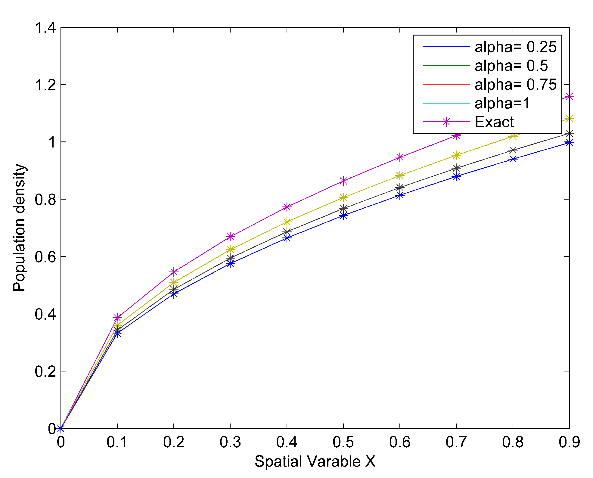
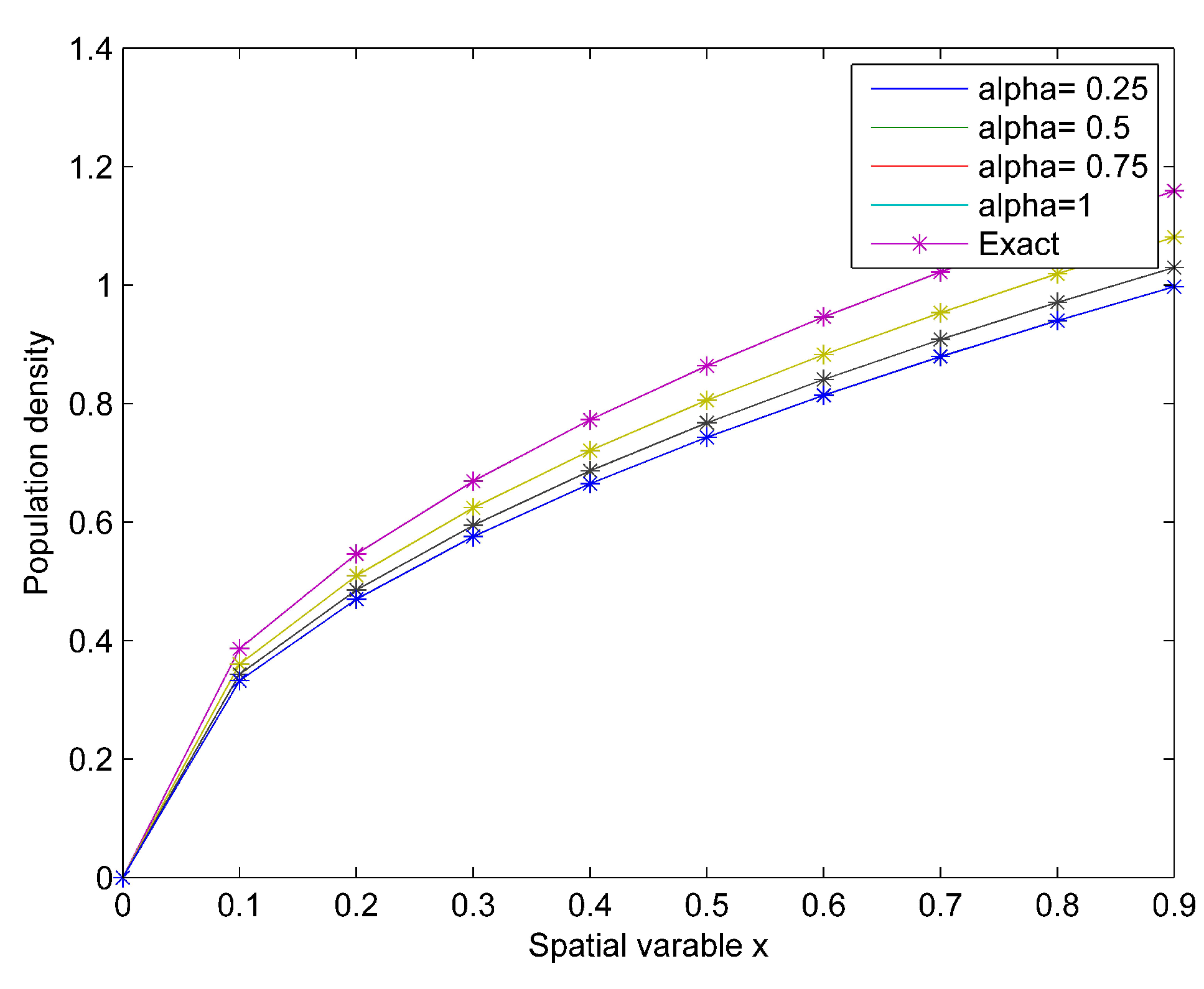
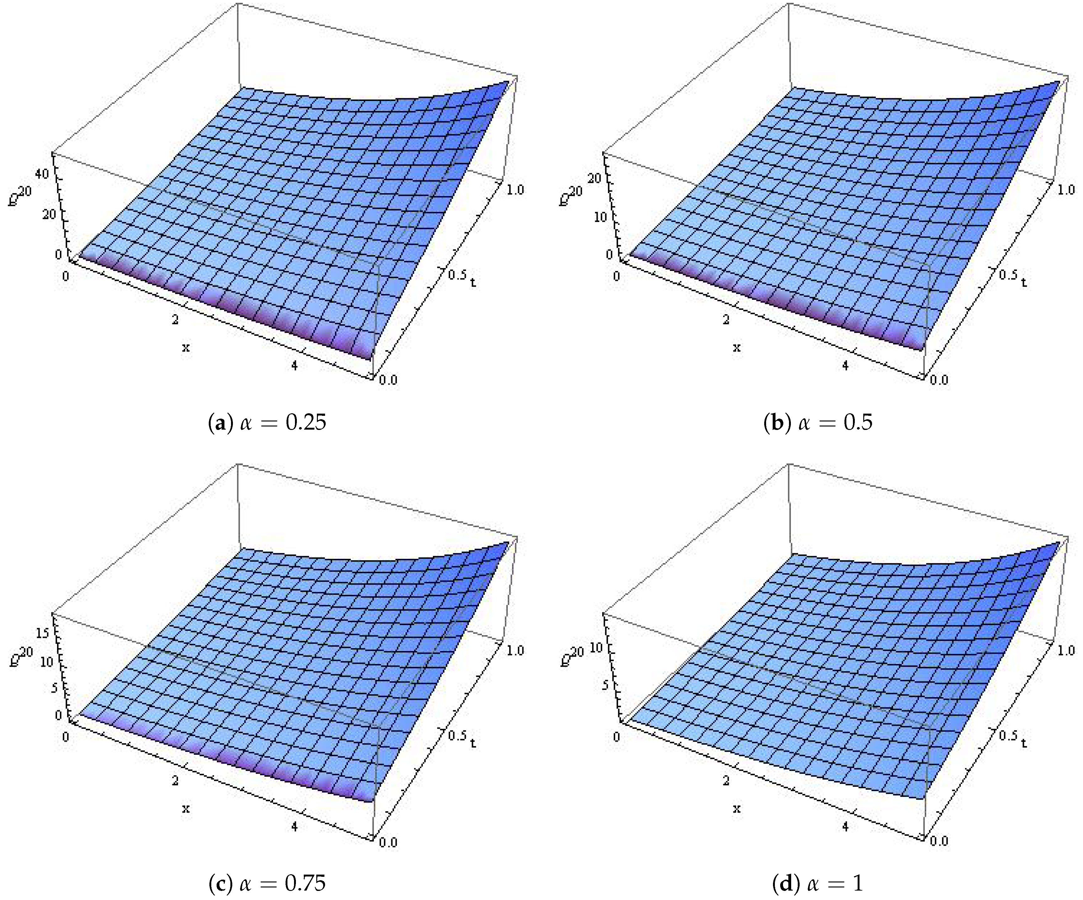
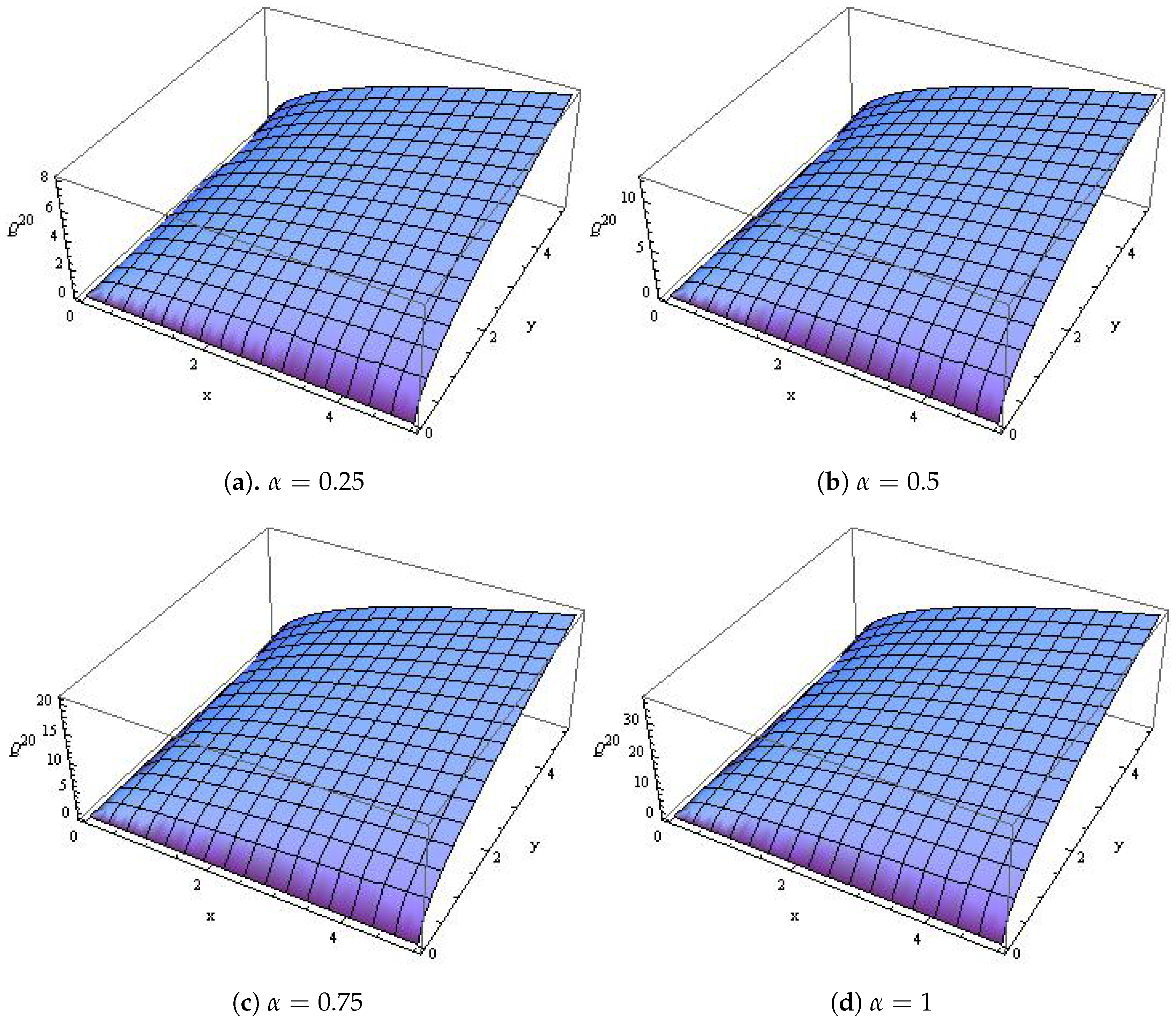
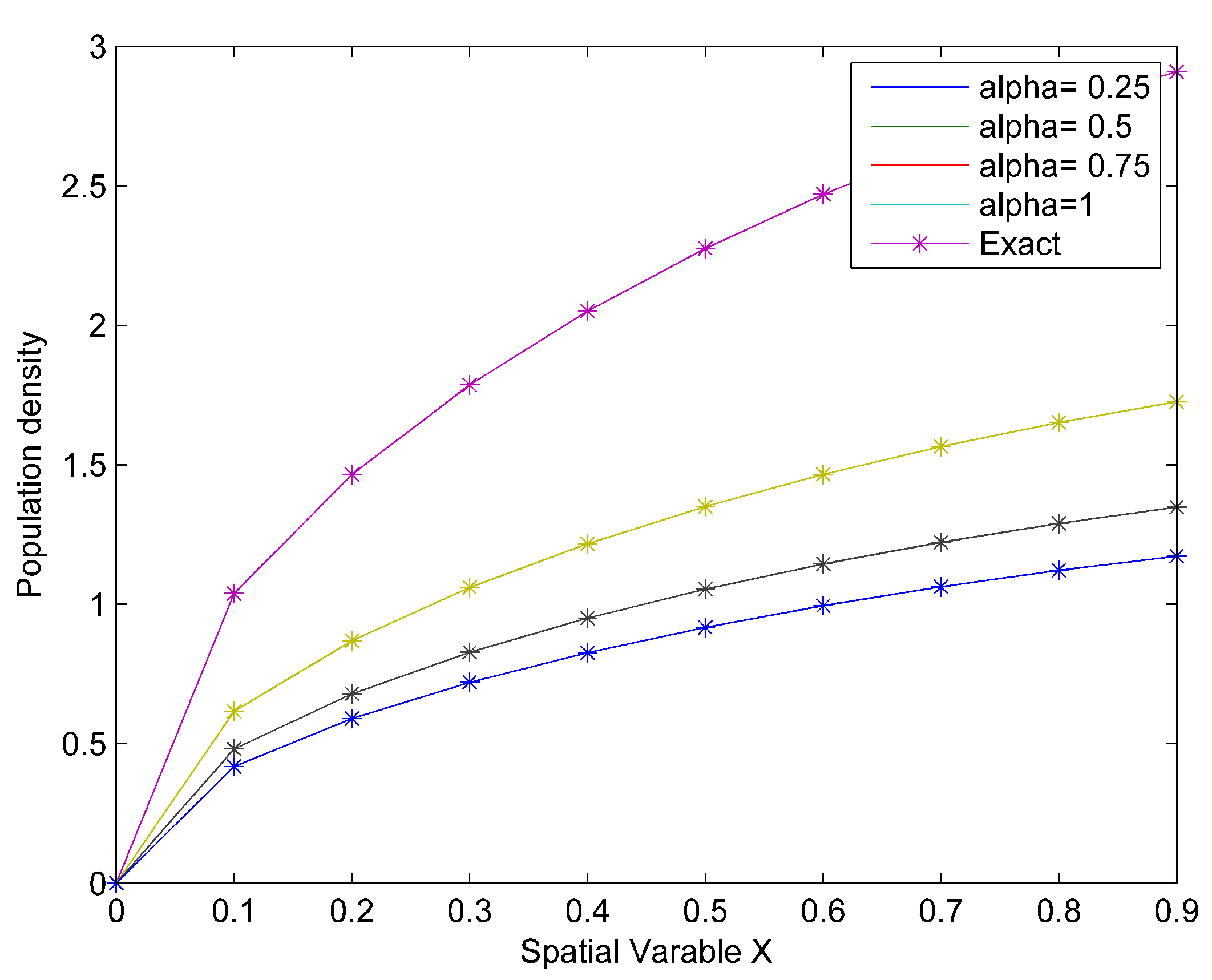
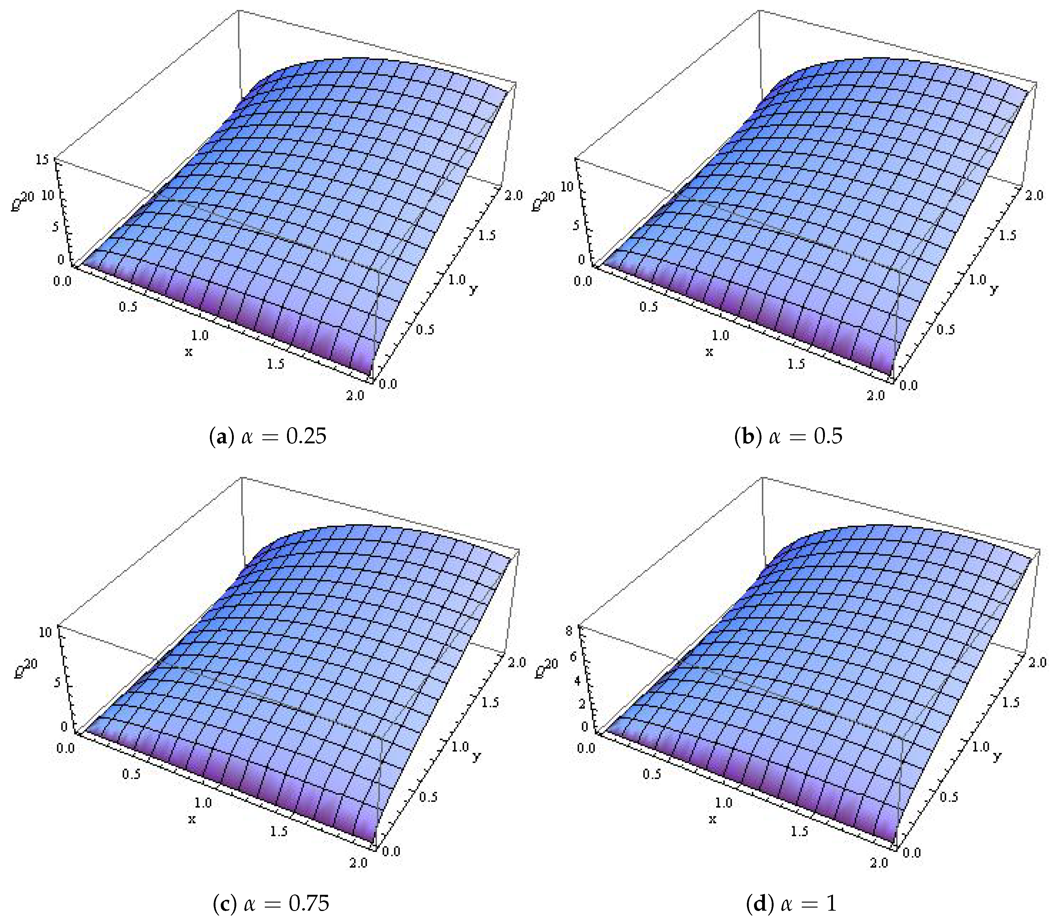
shows the absolute error $E_{abs}=\parallel Q-Q_{10}\parallel$ when $\alpha =0.25,0.5,0.75$ and 1, Figure 1 shows the comparison between the exact solution and the approximate solution while Figure 2 shows the surface plot of the population density when $\alpha =0.25,0.5,0.75$ and $1.$

4.2. Case 2

If $h={\displaystyle \frac{1}{4}},$ $q=1,$ $r=0,$ (Malthusian Law [32] ) and $Q_0\left(x\right)=x^{1/2}$ for one dimensional time-fractional biological population model Equation (1) becomes

$$D_t^{\alpha }Q={\left(Q^2\right)}_{xx}+{\displaystyle \frac{1}{4}}Q,t>0,0<\alpha \le 1,$$

(33)

from case 2, we set

$R\left(Q(x,t)\right)={\displaystyle \frac{1}{4}}Q$,

$N\left(Q(x,t)\right)={\left(Q^2\right)}_{xx}$,

$Q(x,0)=x^{1/2}$.

Using the iterative procedure described in Section 3,

$$Q_0={\mathcal{A}}^{-1}\left[{\displaystyle \frac{1}{{\nu }^{\alpha }}}\left(\sum _{s=0}^{n-1}{\displaystyle \frac{Q^{\left(s\right)}(x,0)}{{\nu }^{2-\alpha +s}}}\right)\right]$$

$$={\mathcal{A}}^{-1}\left[{\displaystyle \frac{Q(x,0)}{{\nu }^2}}\right]$$

(34)

$$=x^{1/2}.$$

$$Q_1={\mathcal{A}}^{-1}\left[{\displaystyle \frac{1}{{\nu }^{\alpha }}}\left(\mathcal{A}\left[R\left(Q_0(x,t)\right)+N\left(Q_0(x,t)\right)\right]\right)\right]$$

$$={\mathcal{A}}^{-1}\left[{\displaystyle \frac{1}{{\nu }^{\alpha }}}\left(\mathcal{A}\left[{\displaystyle \frac{1}{4}}{Q}_0+{\left(Q_0^2\right)}_{xx}\right]\right)\right]$$

(35)

$$=x^{1/2}{\displaystyle \frac{\frac{1}{4}{t}^{\alpha }}{\Gamma (\alpha +1)}}.$$

$$Q_2={\mathcal{A}}^{-1}\left[{\displaystyle \frac{1}{{\nu }^{\alpha }}}\left(\mathcal{A}\left[R\left(Q_1(x,t)\right)+\left\{N(Q_0(x,t)+Q_1(x,t))-N\left(Q_0(x,t)\right)\right\}\right]\right)\right]$$

$$={\mathcal{A}}^{-1}\left[{\displaystyle \frac{1}{{\nu }^{\alpha }}}\left(\mathcal{A}\left[{\displaystyle \frac{1}{4}}{Q}_1+\left\{{\left({(Q_0+Q_1)}^2\right)}_{xx}-{\left(Q_0^2\right)}_{xx}\right\}\right]\right)\right]$$

(36)

$$\begin{gathered} ={\displaystyle \frac{x^{1/2}{\left({\displaystyle \frac{1}{4}}{t}^{\alpha }\right)}^2}{\Gamma (2\alpha +1)}}. \\ ⋮ \end{gathered}$$

$$Q_m={\mathcal{A}}^{-1}\left[{\displaystyle \frac{1}{{\nu }^{\alpha }}}\left(\mathcal{A}\left[R\left(Q_{m-1}(x,t)\right)+\left\{N\left(\sum _{i=0}^{m-1}{Q}_i(x,t)\right)-N\left(\sum _{i=0}^{m-2}{Q}_i(x,t)\right)\right\}\right]\right)\right]$$

$$={\mathcal{A}}^{-1}\left[{\displaystyle \frac{1}{{\nu }^{\alpha }}}\left(\mathcal{A}\left[{\displaystyle \frac{1}{4}}{Q}_{m-1}(x,t)\right]\right)\right]$$

(37)

$$={\displaystyle \frac{x^{1/2}{\left({\displaystyle \frac{1}{4}}{t}^{\alpha }\right)}^m}{\Gamma (m\alpha +1)}}.$$

The m-th order approximate series is derived as

$${\mathcal{Q}}^m(x,t)=\sum _{k=0}^m{Q}_k(x,t)=Q_0(x,t)+Q_1(x,t)+Q_2(x,t)+\cdots +Q_m(x,t)$$

$$=x^{1/2}+{\displaystyle \frac{x^{1/2}{\displaystyle \frac{1}{4}}{t}^{\alpha }}{\Gamma (\alpha +1)}}+{\displaystyle \frac{x^{1/2}{\left({\displaystyle \frac{1}{4}}{t}^{\alpha }\right)}^2}{\Gamma (2\alpha +1)}}+\cdots +{\displaystyle \frac{x^{1/2}{\left({\displaystyle \frac{1}{4}}{t}^{\alpha }\right)}^m}{\Gamma (m\alpha +1)}}$$

$$=x^{1/2}\left({\displaystyle \frac{{\displaystyle \frac{1}{4}}{t}^{\alpha }}{\Gamma (\alpha +1)}}+{\displaystyle \frac{{\left({\displaystyle \frac{1}{4}}{t}^{\alpha }\right)}^2}{\Gamma (2\alpha +1)}}+\cdots +{\displaystyle \frac{{\left({\displaystyle \frac{1}{4}}{t}^{\alpha }\right)}^m}{\Gamma (m\alpha +1)}}\right)$$

(38)

$$=x^{1/2}\sum _{k=0}^m{\displaystyle \frac{{\left({\displaystyle \frac{1}{4}}{t}^{\alpha }\right)}^k}{\Gamma (k\alpha +1)}}.$$

So, the m-th order approximate series solution approach the exact solution as $m\to \infty ,$

$$Q(x,t)=\underset{m\to \infty }{lim}{\mathcal{Q}}^{\left(m\right)}(x,t)$$

$$=x^{1/2}\underset{m\to \infty }{lim}\sum _{k=0}^m{\displaystyle \frac{{\left({\displaystyle \frac{1}{4}}{t}^{\alpha }\right)}^k}{\Gamma (k\alpha +1)}}$$

(39)

$$=x^{1/2}{E}_{\alpha }\left({\displaystyle \frac{1}{4}}{t}^{\alpha }\right),$$

(40)

taking $\alpha =1,$ the exact solution to Equation (33) is

$$Q(x,t)=x^{1/2}{E}_1\left({\displaystyle \frac{1}{4}}t\right)$$

$$=x^{1/2}exp\left({\displaystyle \frac{t}{4}}\right).$$

(41)

Table 3. Absolute error for Case (2) when $t=0.2$.

x	$\mathit{\alpha }=0.25$	$\mathit{\alpha }=0.5$	$\mathit{\alpha }=0.75$	$\mathit{\alpha }=1$
0.1	$5.4\times {10}^{-3}$	$6.2\times {10}^{-7}$	$2.7\times {10}^{-11}$	$4.4\times {10}^{-16}$
0.5	$6.2\times {10}^{-3}$	$7.1\times {10}^{-7}$	$3.1\times {10}^{-11}$	$6.7\times {10}^{-16}$
0.9	$7.1\times {10}^{-3}$	$8.2\times {10}^{-4}$	$3.5\times {10}^{-11}$	$6.7\times {10}^{-16}$

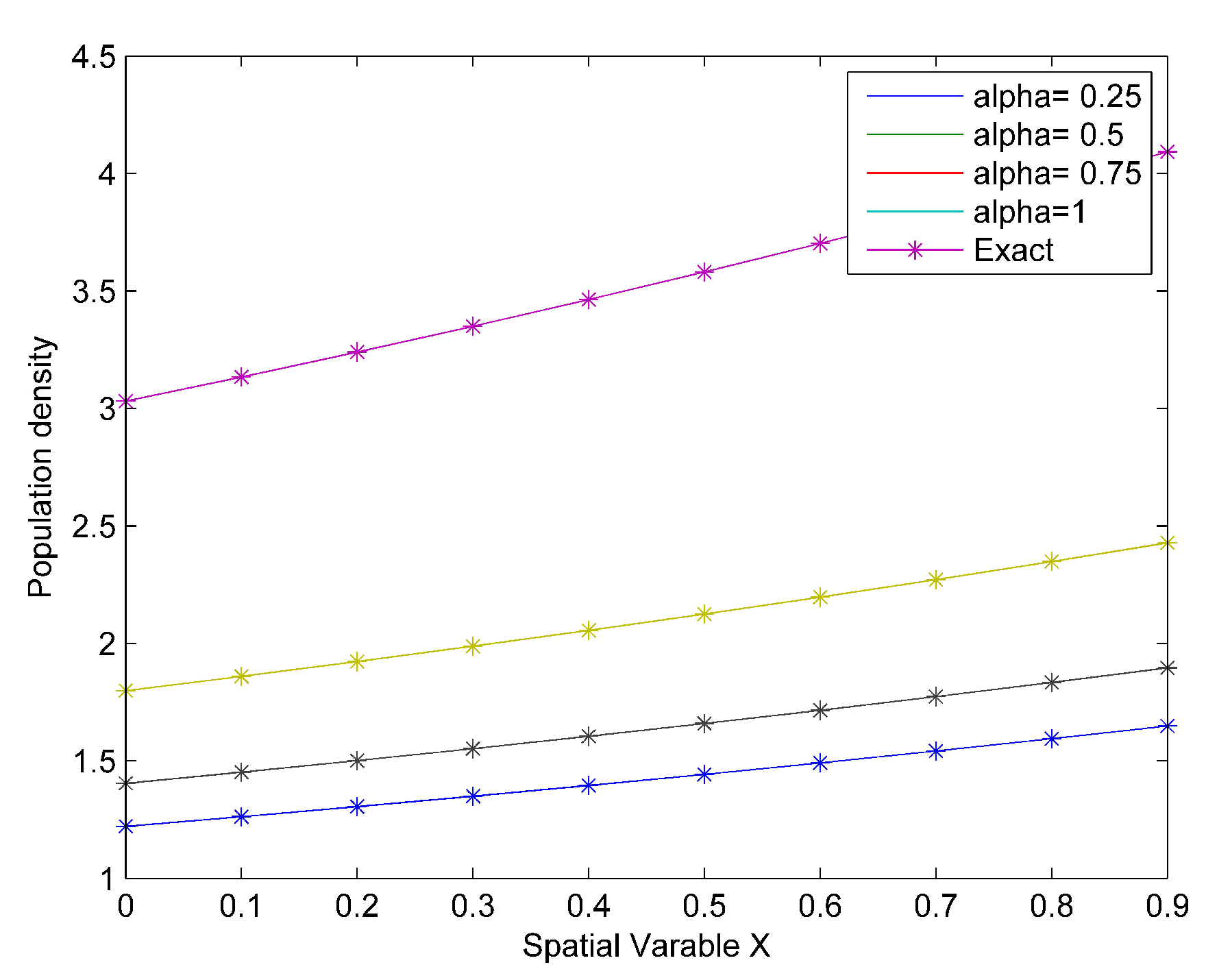
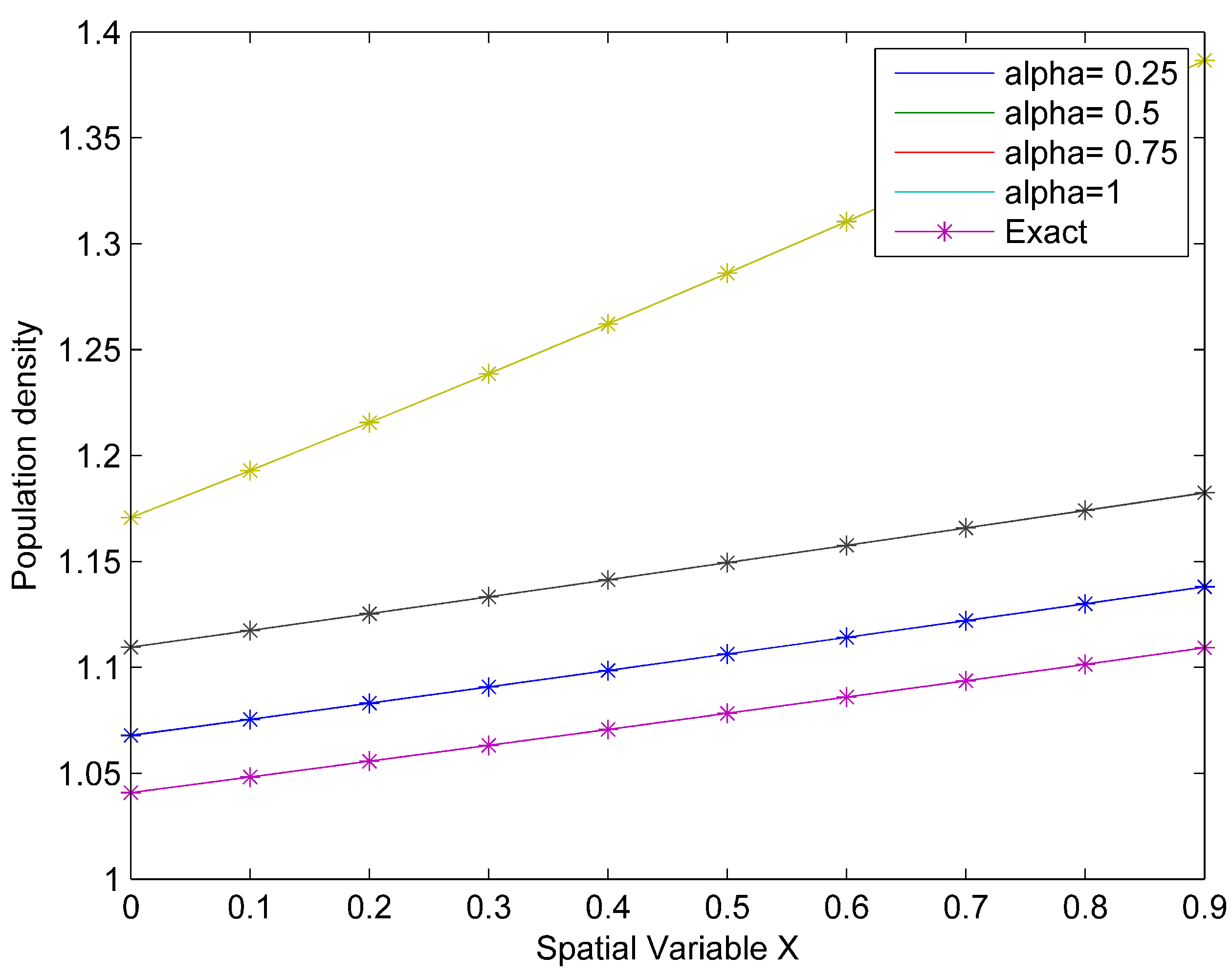
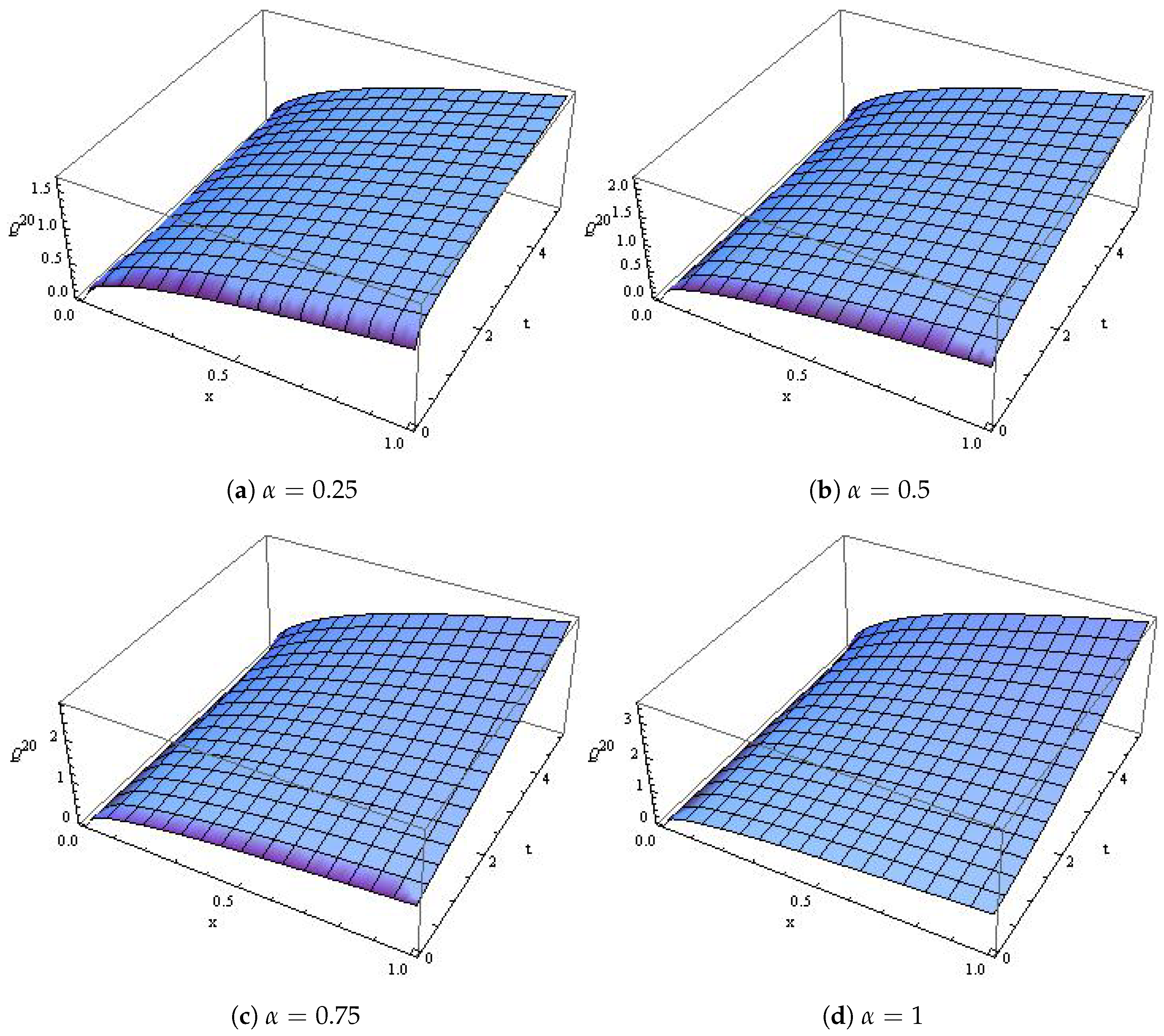
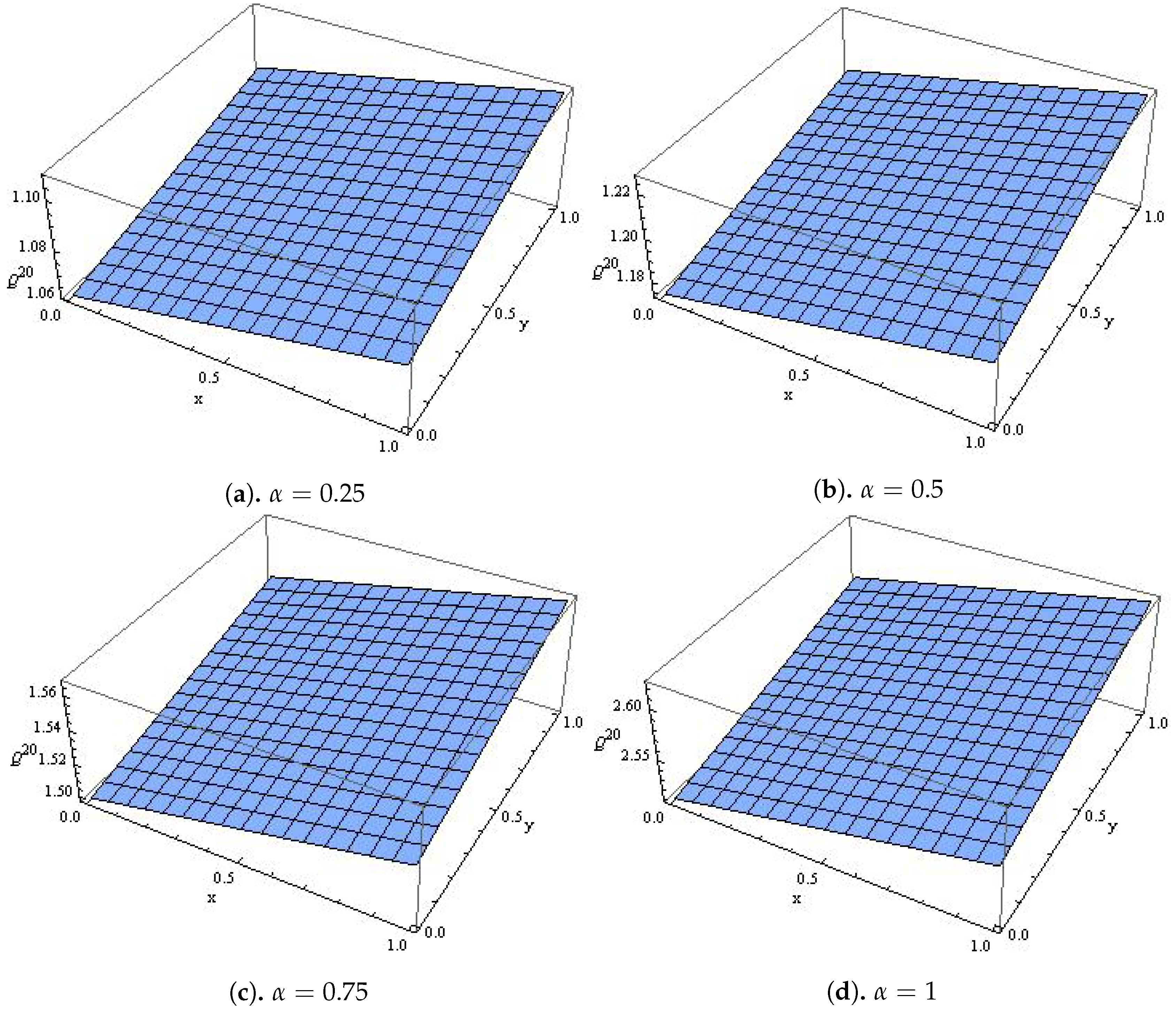
shows the absolute error $E_{abs}=\parallel Q-Q_{10}\parallel$ when $\alpha =0.25,0.5,0.75$ and 1, Figure 3 shows the comparison between the exact solution and the approximate solution while Figure 4 shows the surface plot of the population density when $\alpha =0.25,0.5,0.75$ and $1.$

4.3. Case 3

If $q=1,$ $r=0,$ (Malthusian Law [32] ) and $Q_0(x,y)=\sqrt{xy}$ the time-fractional biological population model Equation (1) becomes

$$D_t^{\alpha }Q={\left(Q^2\right)}_{xx}+{\left(Q^2\right)}_{yy}+hQ,t>0,0<\alpha \le 1,$$

(42)

from case 3, we set

$R\left(Q\right(x,y,t\left)\right)=hQ$,

$N\left(Q(x,y,t)\right)={\left(Q^2\right)}_{xx}+{\left(Q^2\right)}_{yy}$,

$Q(x,y,0)=\sqrt{xy}$.

Using the iterative procedure described in Section 3,

$$Q_0={\mathcal{A}}^{-1}\left[{\displaystyle \frac{1}{{\nu }^{\alpha }}}\left(\sum _{s=0}^{n-1}{\displaystyle \frac{Q^{\left(s\right)}(x,y,0)}{{\nu }^{2-\alpha +s}}}\right)\right]$$

$$={\mathcal{A}}^{-1}\left[{\displaystyle \frac{Q(x,y,0)}{{\nu }^2}}\right]$$

(43)

$$=\sqrt{xy}.$$

$$Q_1={\mathcal{A}}^{-1}\left[{\displaystyle \frac{1}{{\nu }^{\alpha }}}\left(\mathcal{A}\left[R\left(Q_0(x,y,t)\right)+N\left(Q_0(x,y,t)\right)\right]\right)\right]$$

$$={\mathcal{A}}^{-1}\left[{\displaystyle \frac{1}{{\nu }^{\alpha }}}\left(\mathcal{A}\left[h{Q}_0+{\left(Q_0^2\right)}_{xx}+{\left(Q_0^2\right)}_{yy}\right]\right)\right]$$

(44)

$$=\sqrt{xy}{\displaystyle \frac{h{t}^{\alpha }}{\Gamma (\alpha +1)}}.$$

$$Q_2={\mathcal{A}}^{-1}\left[{\displaystyle \frac{1}{{\nu }^{\alpha }}}\left(\mathcal{A}\left[R\left(Q_1(x,y,t)\right)+\left\{N(Q_0(x,y,t)+Q_1(x,y,t))-N\left(Q_0(x,y,t)\right)\right\}\right]\right)\right]$$

$$={\mathcal{A}}^{-1}\left[{\displaystyle \frac{1}{{\nu }^{\alpha }}}\left(\mathcal{A}\left[h{Q}_1+\left\{{\left({(Q_0+Q_1)}^2\right)}_{xx}+{\left({(Q_0+Q_1)}^2\right)}_{yy}-N({\left(Q_0^2\right)}_{xx}+{\left(Q_0^2\right)}_{yy})\right\}\right]\right)\right]$$

(45)

$$\begin{gathered} =\sqrt{xy}{\displaystyle \frac{{\left(h{t}^{\alpha }\right)}^2}{\Gamma (2\alpha +1)}}. \\ ⋮ \end{gathered}$$

$$Q_m={\mathcal{A}}^{-1}\left[{\displaystyle \frac{1}{{\nu }^{\alpha }}}\left(\mathcal{A}\left[R\left(Q_{m-1}(x,y,t)\right)+\left\{N\left(\sum _{i=0}^{m-1}{Q}_i(x,y,t)\right)-N\left(\sum _{i=0}^{m-2}{Q}_i(x,y,t)\right)\right\}\right]\right)\right]$$

$$={\mathcal{A}}^{-1}\left[{\displaystyle \frac{1}{{\nu }^{\alpha }}}\left(\mathcal{A}\left[h{Q}_{m-1}(x,y,t)\right]\right)\right]$$

(46)

$$\sqrt{xy}{\displaystyle \frac{{\left(h{t}^{\alpha }\right)}^m}{\Gamma (m\alpha +1)}}.$$

The m-th order approximate series is derived as

$${\mathcal{Q}}^m(x,y,t)=\sum _{k=0}^m{Q}_k(x,y,t)=Q_0(x,y,t)+Q_1(x,y,t)+Q_2(x,y,t)+\cdots +Q_m(x,y,t)$$

$$=\sqrt{xy}+\sqrt{xy}{\displaystyle \frac{h{t}^{\alpha }}{\Gamma (\alpha +1)}}+\sqrt{xy}{\displaystyle \frac{{\left(h{t}^{\alpha }\right)}^2}{\Gamma (2\alpha +1)}}+\cdots +\sqrt{xy}{\displaystyle \frac{{\left(h{t}^{\alpha }\right)}^m}{\Gamma (m\alpha +1)}}$$

$$=\sqrt{xy}\left(1+{\displaystyle \frac{h{t}^{\alpha }}{\Gamma (\alpha +1)}}+{\displaystyle \frac{{\left(h{t}^{\alpha }\right)}^2}{\Gamma (2\alpha +1)}}+\cdots +{\displaystyle \frac{{\left(h{t}^{\alpha }\right)}^m}{\Gamma (m\alpha +1)}}\right)$$

(47)

$$=\sqrt{xy}\sum _{k=0}^m{\displaystyle \frac{{\left(h{t}^{\alpha }\right)}^k}{\Gamma (k\alpha +1)}}.$$

So, the m-th order approximate series solution approaches the exact solution as $m\to \infty$,

$$Q(x,y,t)=\underset{m\to \infty }{lim}{\mathcal{Q}}^{\left(m\right)}(x,y,t)$$

$$=\sqrt{xy}\underset{m\to \infty }{lim}\sum _{k=0}^m{\displaystyle \frac{{\left(h{t}^{\alpha }\right)}^k}{\Gamma (k\alpha +1)}}$$

(48)

$$=\sqrt{xy}{E}_{\alpha }\left(h{t}^{\alpha }\right),$$

taking $\alpha =1$, the exact solution to Equation (42) is

$$Q(x,y,t)=\sqrt{xy}{E}_1\left(ht\right)$$

$$=\sqrt{xy}exp\left(ht\right),$$

(49)

which is the exact solution to the standard biological population model in [37] when $h=\frac{1}{5}$ and $\alpha =1.$

Table 4. Absolute error for Case (3) when $t=0.2$.

x	y	$\mathit{\alpha }=0.25$	$\mathit{\alpha }=0.5$	$\mathit{\alpha }=0.75$	$\mathit{\alpha }=1$
0.1	0.2	$8.7\times {10}^{-12}$	$1.5\times {10}^{-15}$	0	0
0.1	0.6	$1.5\times {10}^{-11}$	$2.7\times {10}^{-15}$	0	0
0.1	1	$1.9\times {10}^{-11}$	$3.4\times {10}^{-15}$	0	0
0.5	0.2	$1.9\times {10}^{-11}$	$3.4\times {10}^{-15}$	0	0
0.5	0.6	$3.4\times {10}^{-11}$	$5.8\times {10}^{-15}$	0	0
0.5	1	$4.3\times {10}^{-11}$	$7.4\times {10}^{-15}$	0	0
0.9	0.2	$2.6\times {10}^{-11}$	$4.6\times {10}^{-15}$	0	0
0.9	0.6	$4.5\times {10}^{-11}$	$7.8\times {10}^{-15}$	0	0
0.9	1	$5.8\times {10}^{-11}$	$1.0\times {10}^{-14}$	0	0

shows the absolute error $E_{abs}=\parallel Q-Q_{10}\parallel$ when $\alpha =0.25,0.5,0.75$ and 1, Figure 5 shows the comparison between the exact solution and approximate solution while Figure 6 shows the surface plot of the population density when $\alpha =0.25,0.5,0.75$ and $1.$

In

Table 5. Comparison of the absolute error for Case (3) when $t=0.2$.

x	y	Present Method ${\mathit{E}}_{\mathbf{abs}},\mathit{\alpha }=0.5$	Present Method ${\mathit{E}}_{\mathbf{abs}},\mathit{\alpha }=1$	Method in [44] ${\mathit{E}}_{\mathbf{abs}},\mathit{\alpha }=0.5$	Method in [44] ${\mathit{E}}_{\mathbf{abs}},\mathit{\alpha }=1$
0.1	0.2	$1.5\times {10}^{-15}$	0	$1.5\times {10}^{-15}$	$2.7\times {10}^{-17}$
0.1	0.6	$2.6\times {10}^{-15}$	0	$2.6\times {10}^{-15}$	$5.5\times {10}^{-17}$
0.1	1	$3.4\times {10}^{-15}$	0	$3.4\times {10}^{-15}$	$5.5\times {10}^{-17}$
0.5	0.2	$3.4\times {10}^{-15}$	0	$3.4\times {10}^{-15}$	$5.5\times {10}^{-17}$
0.5	0.6	$5.9\times {10}^{-15}$	0	$5.9\times {10}^{-15}$	$1.1\times {10}^{-16}$
0.5	1	$7.4\times {10}^{-15}$	0	$7.6\times {10}^{-15}$	$2.2\times {10}^{-16}$
0.9	0.2	$4.6\times {10}^{-15}$	0	$4.6\times {10}^{-15}$	$2.2\times {10}^{-16}$
0.9	0.6	$7.9\times {10}^{-15}$	0	$7.9\times {10}^{-15}$	$2.2\times {10}^{-16}$
0.9	1	$1.0\times {10}^{-14}$	0	$1.0\times {10}^{-14}$	$2.2\times {10}^{-16}$

, we compared the absolute error of the present method with the method in [44] when $t=0.2$.

4.4. Case 4

If $q=p=1,$ ( Verhulst Law [32] ) and $Q_0(x,y)=exp\left({\displaystyle \frac{1}{2}}\sqrt{{\displaystyle \frac{hr}{2}}}(x+y)\right),$ the time-fractional biological population model Equation (1) becomes

$$D_t^{\alpha }Q={\left(Q^2\right)}_{xx}+{\left(Q^2\right)}_{yy}+hQ(1-rQ),t>0,0<\alpha \le 1,$$

(50)

from case 4, we set

$R\left(Q\right(x,y,t\left)\right)=hQ$,

$N\left(Q(x,y,t)\right)={\left(Q^2\right)}_{xx}+{\left(Q^2\right)}_{yy}-hr{Q}^2$,

$Q(x,y,0)=exp\left({\displaystyle \frac{1}{2}}\sqrt{{\displaystyle \frac{hr}{2}}}(x+y)\right)$.

Using the iterative procedure described in Section 3,

$$Q_0={\mathcal{A}}^{-1}\left[{\displaystyle \frac{1}{{\nu }^{\alpha }}}\left(\sum _{s=0}^{n-1}{\displaystyle \frac{Q^{\left(s\right)}(x,y,0)}{{\nu }^{2-\alpha +s}}}\right)\right]$$

$$={\mathcal{A}}^{-1}\left[{\displaystyle \frac{Q(x,y,0)}{{\nu }^2}}\right]$$

(51)

$$=exp\left({\displaystyle \frac{1}{2}}\sqrt{{\displaystyle \frac{hr}{2}}}(x+y)\right).$$

$$Q_1={\mathcal{A}}^{-1}\left[{\displaystyle \frac{1}{{\nu }^{\alpha }}}\left(\mathcal{A}\left[R\left(Q_0(x,y,0)\right)+N\left(Q_0(x,y,0)\right)\right]\right)\right]$$

$$={\mathcal{A}}^{-1}\left[{\displaystyle \frac{1}{{\nu }^{\alpha }}}\left(\mathcal{A}\left[h{Q}_0+{\left(Q_0^2\right)}_{xx}+{\left(Q_0^2\right)}_{yy}-hr{Q}_0^2\right]\right)\right]$$

(52)

$$=exp\left({\displaystyle \frac{1}{2}}\sqrt{{\displaystyle \frac{hr}{2}}}(x+y)\right){\displaystyle \frac{h{t}^{\alpha }}{\Gamma (\alpha +1)}}.$$

$$Q_2={\mathcal{A}}^{-1}\left[{\displaystyle \frac{1}{{\nu }^{\alpha }}}\left(\mathcal{A}\left[R\left(Q_1(x,y,0)\right)+\left\{N\left(Q_0(x,y,t)+Q_1(x,y,t)\right)-N\left(Q_0(x,y,t)\right)\right\}\right]\right)\right]$$

$$\begin{array}{c}={\mathcal{A}}^{-1}\left[{\displaystyle \frac{1}{{\nu }^{\alpha }}}\left(\mathcal{A}\left[h{Q}_1\right]\right)\right]+\hfill \\ \hfill {\mathcal{A}}^{-1}\left[{\displaystyle \frac{1}{{\nu }^{\alpha }}}\left(\mathcal{A}\left[({\left({(Q_0+Q_1)}^2\right)}_{xx}+{\left({(Q_0+Q_1)}^2\right)}_{yy}-hr{(Q_0+Q_1)}^2)-({\left(Q_0^2\right)}_{xx}+{\left(Q_0^2\right)}_{yy}-hr{Q}_0^2)\right]\right)\right]\end{array}$$

(53)

$$\begin{gathered} =exp\left({\displaystyle \frac{1}{2}}\sqrt{{\displaystyle \frac{hr}{2}}}(x+y)\right){\displaystyle \frac{{\left(h{t}^{\alpha }\right)}^2}{\Gamma (2\alpha +1)}}. \\ ⋮ \end{gathered}$$

$$Q_m={\mathcal{A}}^{-1}\left[{\displaystyle \frac{1}{{\nu }^{\alpha }}}\left(\mathcal{A}\left[R\left(Q_{m-1}(x,y,t)\right)+\left\{N\left(\sum _{i=0}^{m-1}{Q}_i(x,y,t)\right)-N\left(\sum _{i=0}^{m-2}{Q}_i(x,y,t)\right)\right\}\right]\right)\right]$$

$$={\mathcal{A}}^{-1}\left[{\displaystyle \frac{1}{{\nu }^{\alpha }}}\left(\mathcal{A}\left[h{Q}_{m-1}(x,y,t)\right]\right)\right]$$

(54)

$$=exp\left({\displaystyle \frac{1}{2}}\sqrt{{\displaystyle \frac{hr}{2}}}(x+y)\right){\displaystyle \frac{{\left(h{t}^{\alpha }\right)}^m}{\Gamma (m\alpha +1)}}.$$

The m-th order approximate series is derived as

$${\mathcal{Q}}^m(x,y,t)=\sum _{k=0}^m{Q}_k(x,y,t)=Q_0(x,y,t)+Q_1(x,y,t)+Q_2(x,y,t)+\cdots +Q_m(x,y,t)$$

$$\begin{array}{c}=exp\left({\displaystyle \frac{1}{2}}\sqrt{{\displaystyle \frac{hr}{2}}}(x+y)\right)+exp\left({\displaystyle \frac{1}{2}}\sqrt{{\displaystyle \frac{hr}{2}}}(x+y)\right){\displaystyle \frac{h{t}^{\alpha }}{\Gamma (\alpha +1)}}+\hfill \\ \hfill exp\left({\displaystyle \frac{1}{2}}\sqrt{{\displaystyle \frac{hr}{2}}}(x+y)\right){\displaystyle \frac{{\left(h{t}^{\alpha }\right)}^2}{\Gamma (2\alpha +1)}}+\cdots +exp\left({\displaystyle \frac{1}{2}}\sqrt{{\displaystyle \frac{hr}{2}}}(x+y)\right){\displaystyle \frac{{\left(h{t}^{\alpha }\right)}^m}{\Gamma (m\alpha +1)}}\end{array}$$

$$=exp\left({\displaystyle \frac{1}{2}}\sqrt{{\displaystyle \frac{hr}{2}}}(x+y)\right)\left(1+{\displaystyle \frac{h{t}^{\alpha }}{\Gamma (\alpha +1)}}+{\displaystyle \frac{{\left(h{t}^{\alpha }\right)}^2}{\Gamma (2\alpha +1)}}+\cdots +{\displaystyle \frac{{\left(h{t}^{\alpha }\right)}^m}{\Gamma (m\alpha +1)}}\right)$$

(55)

$$=exp\left({\displaystyle \frac{1}{2}}\sqrt{{\displaystyle \frac{hr}{2}}}(x+y)\right)\sum _{k=0}^m{\displaystyle \frac{{\left(h{t}^{\alpha }\right)}^k}{\Gamma (k\alpha +1)}}.$$

So, the m-th order approximate series solution approach the exact solution as $m\to \infty$,

$$Q(x,y,t)=\underset{m\to \infty }{lim}{\mathcal{Q}}^{\left(m\right)}(x,y,t)$$

$$=exp\left({\displaystyle \frac{1}{2}}\sqrt{{\displaystyle \frac{hr}{2}}}(x+y)\right)\underset{m\to \infty }{lim}\sum _{k=0}^m{\displaystyle \frac{{\left(h{t}^{\alpha }\right)}^k}{\Gamma (k\alpha +1)}}$$

(56)

$$=exp\left({\displaystyle \frac{1}{2}}\sqrt{{\displaystyle \frac{hr}{2}}}(x+y)\right)E_{\alpha }\left(h{t}^{\alpha }\right)$$

taking $\alpha =1$, the exact solution to Equation (50) is

$$=exp\left({\displaystyle \frac{1}{2}}\sqrt{{\displaystyle \frac{hr}{2}}}(x+y)\right)E_1\left(ht\right)$$

$$=exp\left({\displaystyle \frac{1}{2}}\sqrt{{\displaystyle \frac{hr}{2}}}(x+y)+ht\right),$$

(57)

which is the exact solution to the biological population model in [36] when $h=1.$

Table 6. Absolute error for Case (4) when $t=0.2$.

x	y	$\mathit{\alpha }=0.25$	$\mathit{\alpha }=0.5$	$\mathit{\alpha }=0.75$	$\mathit{\alpha }=1$
0.1	0.2	$6.4\times {10}^{-11}$	$1.1\times {10}^{-14}$	0	0
0.1	0.6	$6.9\times {10}^{-11}$	$1.2\times {10}^{-14}$	0	0
0.1	1	$7.3\times {10}^{-11}$	$1.3\times {10}^{-14}$	0	0
0.5	0.2	$6.9\times {10}^{-11}$	$1.2\times {10}^{-14}$	0	0
0.5	0.6	$7.3\times {10}^{-11}$	$1.3\times {10}^{-14}$	0	0
0.5	1	$7.8\times {10}^{-11}$	$1.4\times {10}^{-14}$	0	0
0.9	0.2	$7.3\times {10}^{-11}$	$1.2\times {10}^{-14}$	0	0
0.9	0.6	$7.8\times {10}^{-11}$	$1.4\times {10}^{-14}$	0	0
0.9	1	$8.3\times {10}^{-11}$	$1.4\times {10}^{-14}$	0	0

shows the absolute error $E_{abs}=\parallel Q-Q_{10}\parallel$ when $\alpha =0.25,0.5,0.75$ and 1, Figure 7 shows the comparison between the exact solution and approximate solution while Figure 8 shows the surface plot of the population density when $\alpha =0.25,0.5,0.75$ and $1.$

4.5. Case 5

If $h=1,$ $r=0$ and $Q_0(x,y)={\left(Sin\left(x\right)Sinh\left(y\right)\right)}^{1/2},$ the time-fractional biological population model Equation (1) becomes

$$D_t^{\alpha }Q={\left(Q^2\right)}_{xx}+{\left(Q^2\right)}_{yy}+Q,t>0,0<\alpha \le 1,$$

(58)

from case 4, we set

$R\left(Q\right(x,y,t\left)\right)=Q$,

$N\left(Q(x,y,t)\right)={\left(Q^2\right)}_{xx}+{\left(Q^2\right)}_{yy}$,

$Q(x,y,0)={\left(Sin\left(x\right)Sinh\left(y\right)\right)}^{1/2}$.

Using the iterative procedure described in Section 3,

$$Q_0={\mathcal{A}}^{-1}\left[{\displaystyle \frac{1}{{\nu }^{\alpha }}}\left(\sum _{s=0}^{n-1}{\displaystyle \frac{Q^{\left(s\right)}(x,y,0)}{{\nu }^{2-\alpha +s}}}\right)\right]$$

$$={\mathcal{A}}^{-1}\left[{\displaystyle \frac{Q(x,y,0)}{{\nu }^2}}\right]$$

(59)

$$={\left(Sin\left(x\right)Sinh\left(y\right)\right)}^{1/2}.$$

$$Q_1={\mathcal{A}}^{-1}\left[{\displaystyle \frac{1}{{\nu }^{\alpha }}}\left(\mathcal{A}\left[R\left(Q_0(x,y,0)\right)+N\left(Q_0(x,y,0)\right)\right]\right)\right]$$

$$={\mathcal{A}}^{-1}\left[{\displaystyle \frac{1}{{\nu }^{\alpha }}}\left(\mathcal{A}\left[Q_0+{\left(Q_0^2\right)}_{xx}+{\left(Q_0^2\right)}_{yy}\right]\right)\right]$$

(60)

$$={\left(Sin\left(x\right)Sinh\left(y\right)\right)}^{1/2}{\displaystyle \frac{t^{\alpha }}{\Gamma (\alpha +1)}}.$$

$$Q_2={\mathcal{A}}^{-1}\left[{\displaystyle \frac{1}{{\nu }^{\alpha }}}\left(\mathcal{A}\left[R\left(Q_0(x,y,t)\right)+\left\{N(Q_0(x,y,t)+Q_1(x,y,t))-N\left(Q_0(x,y,t)\right)\right\}\right]\right)\right]$$

$$={\mathcal{A}}^{-1}\left[{\displaystyle \frac{1}{{\nu }^{\alpha }}}\left(\mathcal{A}\left[Q_1+\left\{{\left({(Q_0+Q_1)}^2\right)}_{xx}+{\left({(Q_0+Q_1)}^2\right)}_{yy}-({\left(Q_0^2\right)}_{xx}+{\left(Q_0^2\right)}_{yy})\right\}\right]\right)\right]$$

(61)

$$\begin{gathered} ={\left(Sin\left(x\right)Sinh\left(y\right)\right)}^{1/2}{\displaystyle \frac{t^{2\alpha }}{\Gamma (2\alpha +1)}}. \\ ⋮ \end{gathered}$$

$$Q_m={\mathcal{A}}^{-1}\left[{\displaystyle \frac{1}{{\nu }^{\alpha }}}\left(\mathcal{A}\left[R\left(Q_{m-1}(x,y,t)\right)+\left\{N\left(\sum _{i=0}^{m-1}{Q}_i(x,y,t)\right)-N\left(\sum _{i=0}^{m-2}{Q}_i(x,y,t)\right)\right\}\right]\right)\right]$$

$$={\mathcal{A}}^{-1}\left[{\displaystyle \frac{1}{{\nu }^{\alpha }}}\left(\mathcal{A}\left[Q_{m-1}(x,y,t)\right]\right)\right]$$

(62)

$$={\left(Sin\left(x\right)Sinh\left(y\right)\right)}^{1/2}{\displaystyle \frac{t^{m\alpha }}{\Gamma (m\alpha +1)}}.$$

The m-th order approximate series is derived as

$${\mathcal{Q}}^m(x,y,t)=\sum _{k=0}^m{Q}_k(x,y,t)=Q_0(x,y,t)+Q_1(x,y,t)+Q_2(x,y,t)+\cdots +Q_m(x,y,t)$$

$$={\left(Sin\left(x\right)Sinh\left(y\right)\right)}^{1/2}\left(1+{\displaystyle \frac{t^{\alpha }}{\Gamma (\alpha +1)}}+{\displaystyle \frac{t^{2\alpha }}{\Gamma (2\alpha +1)}}+\cdots +{\displaystyle \frac{t^{m\alpha }}{\Gamma (m\alpha +1)}}\right)$$

(63)

$$={\left(Sin\left(x\right)Sinh\left(y\right)\right)}^{1/2}\sum _{k=0}^m{\displaystyle \frac{t^{t\alpha }}{\Gamma (k\alpha +1)}}.$$

So, the m-th order approximate series solution approach the exact solution as $m\to \infty$,

$$Q(x,y,t)=\underset{m\to \infty }{lim}{\mathcal{Q}}^{\left(m\right)}(x,y,t)$$

$$={\left(Sin\left(x\right)Sinh\left(y\right)\right)}^{1/2}\underset{m\to \infty }{lim}\sum _{k=0}^m{\displaystyle \frac{t^{k\alpha }}{\Gamma (k\alpha +1)}}$$

(64)

$$={\left(Sin\left(x\right)Sinh\left(y\right)\right)}^{1/2}{E}_{\alpha }\left(t^{\alpha }\right),$$

taking $\alpha =1$, the exact solution to Equation (58) is

$$Q(x,y,t)={\left(Sin\left(x\right)Sinh\left(y\right)\right)}^{1/2}{E}_1\left(t\right)$$

$$={\left(Sin\left(x\right)Sinh\left(y\right)\right)}^{1/2}exp\left(t\right),$$

(65)

which is the exact solution to the biological population model in [45].

Table 7. Absolute error for Case (5) when $t=0.2$.

x	y	$\mathit{\alpha }=0.25$	$\mathit{\alpha }=0.5$	$\mathit{\alpha }=0.75$	$\mathit{\alpha }=1$
0.1	0.2	$7.4\times {10}^{-4}$	$8.6\times {10}^{-8}$	$3.7\times {10}^{-12}$	$5.6\times {10}^{-17}$
0.1	0.6	$1.3\times {10}^{-3}$	$1.5\times {10}^{-7}$	$6.6\times {10}^{-12}$	$1.1\times {10}^{-16}$
0.1	1	$1.8\times {10}^{-3}$	$2.1\times {10}^{-7}$	$9.0\times {10}^{-12}$	$1.1\times {10}^{-16}$
0.5	0.2	$1.6\times {10}^{-3}$	$1.9\times {10}^{-7}$	$8.2\times {10}^{-12}$	$1.7\times {10}^{-16}$
0.5	0.6	$2.9\times {10}^{-3}$	$3.3\times {10}^{-7}$	$1.4\times {10}^{-11}$	$2.2\times {10}^{-16}$
0.5	1	$3.9\times {10}^{-3}$	$4.5\times {10}^{-7}$	$2.0\times {10}^{-11}$	$3.3\times {10}^{-16}$
0.9	0.2	$2.1\times {10}^{-3}$	$2.4\times {10}^{-7}$	$1.0\times {10}^{-11}$	$1.7\times {10}^{-16}$
0.9	0.6	$3.7\times {10}^{-3}$	$4.3\times {10}^{-7}$	$1.9\times {10}^{-11}$	$3.3\times {10}^{-16}$
0.9	1	$5.1\times {10}^{-3}$	$5.8\times {10}^{-7}$	$2.5\times {10}^{-11}$	$4.4\times {10}^{-16}$

shows the absolute error $E_{abs}=\parallel Q-Q_{10}\parallel$ when $\alpha =0.25,0.5,0.75$ and 1, Figure 9 shows the comparison between the exact and approximate solutions while Figure 10 shows the surface plot of the population density when $\alpha =0.25,0.5,0.75$ and $1.$

In

Table 8. Comparison of the absolute error for Case (5) when $t=0.2$.

x	y	Present Method ${\mathit{E}}_{\mathbf{abs}},\mathit{\alpha }=0.5$	Present Method ${\mathit{E}}_{\mathbf{abs}},\mathit{\alpha }=1$	Method in [44] ${\mathit{E}}_{\mathbf{abs}},\mathit{\alpha }=0.5$	Method in [44] ${\mathit{E}}_{\mathbf{abs}},\mathit{\alpha }=1$
0.1	0.2	$8.6\times {10}^{-8}$	$5.6\times {10}^{-17}$	$8.6\times {10}^{-8}$	$5.6\times {10}^{-17}$
0.1	0.6	$1.5\times {10}^{-7}$	$1.1\times {10}^{-16}$	$1.5\times {10}^{-7}$	$1.1\times {10}^{-16}$
0.1	1	$2.1\times {10}^{-7}$	$1.1\times {10}^{-16}$	$2.1\times {10}^{-7}$	$1.1\times {10}^{-16}$
0.5	0.2	$1.9\times {10}^{-7}$	$1.7\times {10}^{-16}$	$1.9\times {10}^{-7}$	$1.7\times {10}^{-16}$
0.5	0.6	$3.3\times {10}^{-7}$	$2.2\times {10}^{-16}$	$3.3\times {10}^{-7}$	$2.2\times {10}^{-16}$
0.5	1	$4.5\times {10}^{-7}$	$3.3\times {10}^{-16}$	$4.5\times {10}^{-7}$	$3.3\times {10}^{-16}$
0.9	0.2	$2.4\times {10}^{-7}$	$1.7\times {10}^{-16}$	$2.4\times {10}^{-7}$	$1.7\times {10}^{-16}$
0.9	0.6	$4.3\times {10}^{-7}$	$3.3\times {10}^{-16}$	$4.3\times {10}^{-7}$	$3.3\times {10}^{-16}$
0.9	1	$5.8\times {10}^{-7}$	$4.4\times {10}^{-16}$	$5.8\times {10}^{-7}$	$4.4\times {10}^{-16}$

, we compared the absolute error of the present method with the method in [44] when $t=0.2$.

5. Conclusions

In this paper, we used the Aboodh transform iterative method to obtain the approximate analytical solutions of one and two dimensions fractional biological population models. To the best of our knowledge, no attempt has been made regarding the approximate analytical solution of fractional biological population models using the Aboodh transform iterative method which is the novelty of this study. We observed that the series form solutions converged to the exact solutions which agree strongly with the results in [37,44,45]. The graphical solution of Figure 1, Figure 2, Figure 3, Figure 4, Figure 5, Figure 6, Figure 7, Figure 8, Figure 9 and Figure 10 and Table 2, Table 3, Table 4, Table 5, Table 6, Table 7 and Table 8 revealed that the solutions depends not only on the time t but also on the fractional-order $\alpha$. The population density increases with the spatial variables and time, an indication that the fractional model complements the anomalous biological diffusion behavior observed in the field. Figure 1, Figure 3, Figure 5, Figure 7 and Figure 9 showed that the exact and approximate series solutions were nearly identical for different values of $\alpha .$ However, the approximate series solution can be improved by increasing the values of $m.$ Finally, the easy implementation of the proposed method suggests that it can be modified for the solutions of other fractional partial differential equations arising in applied science. In the future, the authors intend to study the stability and error analysis of the proposed method.

References

1. Pinto, C.M.; Carvalho, A.R. Diabetes mellitus and TB co-existence: Clinical implications from a fractional order modelling. Appl. Math. Model. 2019, 68, 219–243. [Google Scholar] [CrossRef]
2. Kumar, D.; Singh, J.; Tanwar, K.; Baleanu, D. A new fractional exothermic reactions model having constant heat source in porous media with power, exponential and Mittag-Leffler laws. Int. J. Heat Mass Transf. 2019, 138, 1222–1227. [Google Scholar] [CrossRef]
3. Kumar, D.; Singh, J.; Baleanu, D. On the analysis of vibration equation involving a fractional derivative with Mittag-Leffler law. Math. Methods Appl. Sci. 2020, 43, 443–457. [Google Scholar] [CrossRef]
4. Kumar, D.; Singh, J.; Al Qurashi, M.; Baleanu, D. A new fractional SIRS-SI malaria disease model with application of vaccines, antimalarial drugs, and spraying. Adv. Differ. Equ. 2019, 1, 278. [Google Scholar] [CrossRef] [Green Version]
5. Kumar, D.; Singh, J.; Al Qurashi, M.; Baleanu, D. A hybrid analytical algorithm for nonlinear fractional wave-like equations. Math. Model. Nat. Phenom. 2019, 14, 304. [Google Scholar] [CrossRef] [Green Version]
6. Goswami, A.; Singh, J.; Kumar, D. An efficient analytical approach for fractional equal width equations describing hydro-magnetic waves in cold plasma. Phys. Stat. Mech. Appl. 2019, 524, 563–575. [Google Scholar] [CrossRef]
7. Podlubny, I. Fractional Differential Equations: An Introduction to Fractional Derivatives, Fractional Differential Equations, to Methods of Their Solution and Some of Their Applications; Elsevier: Amsterdam, The Netherlands, 1998. [Google Scholar]
8. Oldham, K.; Spanier, J. The Fractional Calculus Theory and Applications of Differentiation and Integration to Arbitrary Order; Academic Press: New York, NY, USA, 1974. [Google Scholar]
9. Miller, K.S.; Ross, B. An Introduction to the Fractional Calculus and Fractional Differential Equations; Wiley: New York, NY, USA, 1993. [Google Scholar]
10. Kilbas, A.A.A.; Srivastava, H.M.; Trujilo, J.J. Theory and Applications of Fractional Differential Equations; Elsevier: Amsterdam, The Netherlands, 2006; Volume 204. [Google Scholar]
11. Diethelm, K. The Analysis of Fractional Differential Equations: An Application-Oriented Exposition Using Differential Operators of Caputo Type; Springer Science and Business Media: Berlin/Heidelberg, Germany, 2010. [Google Scholar]
12. Debnath, L.; Bhatta, D. Integral Transforms and Their Applications; CRC Press: Boca Raton, FL, USA, 2014. [Google Scholar]
13. Watugula, G.K. A New Integral Transform to Solve Differential Equations and Control Engineering Problems. Int. J. Math. Educ. Sxience Technol. 1993, 24, 409–421. [Google Scholar] [CrossRef]
14. Khan, Z.H.; Khan, W.A. Natural transform-Properties and applications. NUST J. Eng. Sci. 2008, 1, 127–133. [Google Scholar]
15. Elzaki, T.M. The new integral transform Elzaki transform. Glob. J. Pure Appl. Math. 2011, 7, 57–64. [Google Scholar]
16. Aboodh, K.S. The new integral transform Aboodh transform. Glob. J. Pure Appl. Math. 2013, 9, 35–43. [Google Scholar]
17. Maitama, S.; Weidong, Z. New Integral Transform: Shehu Transform a Generalization of Sumudu and Laplace Transform for Solving Differential Equations. Int. J. Anal. Appl. 2019, 17, 167–190. [Google Scholar]
18. Saadeh, R.; Ahmad, Q.; Aliaa, B. A New Integral Transform: ARA Transform and its Properties and Applications. Symmetry 2020, 12, 925. [Google Scholar] [CrossRef]
19. Daftardar-Gejji, V.; Jafari, H. An Iterative Method for Solving Nonlinear Functional Equations. J. Math. Anal. Appl. 2006, 316, 753–763. [Google Scholar] [CrossRef] [Green Version]
20. Xu, F.; Gao, Y.; Zhang, W. Construction of analytic solution for time-fractional Boussinesq equation using iterative method. Adv. Math. Phys. 2015, 2015. [Google Scholar] [CrossRef]
21. Daftardar-Gejji, V.; Bhalekar, S. Solving fractional boundary value problems with Dirichlet boundary conditions using a new iterative method. Comput. Math. Appl. 2010, 59, 1801–1809. [Google Scholar] [CrossRef] [Green Version]
22. Bhalekar, S.; Daftardar-Gejji, V. Solving evolution equations using a new iterative method. Numer. Methods Partial. Differ. Equ. Int. J. 2010, 26, 906–916. [Google Scholar] [CrossRef]
23. Bhalekar, S.; Daftardar-Gejji, V. New iterative method: Application to partial differential equations. Appl. Math. Comput. 2008, 203, 778–783. [Google Scholar] [CrossRef]
24. Li, W.; Pang, Y. An iterative method for time-fractional Swift-Hohenberg equation. Adv. Math. Phys. 2018, 1–13. [Google Scholar] [CrossRef]
25. Naik, P.A.; Zu, J.; Owolabi, K.M. Global dynamics of a fractional order model for the transmission of HIV epidemic with optimal control. Chaos Solitons Fractals 2020, 138, 109826. [Google Scholar] [CrossRef]
26. Naik, P.A. Global dynamics of a fractional-order SIR epidemic model with memory. Int. J. Biomath. 2020, 2050071. [Google Scholar] [CrossRef]
27. Noeiaghdam, S.; Sidorov, D. Caputo-Fabrizio Fractional Derivative to Solve the Fractional Model of Energy Supply-Demand System. Math. Model. Eng. Probl. 2020, 7, 359–367. [Google Scholar] [CrossRef]
28. Yavuz, M.; Özdemir, N. Analysis of an epidemic spreading model with exponential decay law. Math. Sci. Appl. Notes 2020, 8, 142–154. [Google Scholar] [CrossRef] [Green Version]
29. Sene, N. Fractional SIRI Model with Delay in Context of the Generalized Liouville–Caputo Fractional Derivative; CRC Press: Boca Raton, FL, USA, 2020. [Google Scholar]
30. El-Sayed, A.M.A.; Rida, S.Z.; Arafa, A.A.M. Exact solutions of fractional-order biological population model. Commun. Theor. Phys. 2009, 52, 992–996. [Google Scholar] [CrossRef]
31. Lu, Y.G. Hölder estimates of solutions of biological population equations. Appl. Math. Lett. 2000, 13, 123–126. [Google Scholar] [CrossRef] [Green Version]
32. Gurtin, M.E.; MacCamy, R.C. On the diffusion of biological populations. Math. Biosci. 1977, 3, 35–49. [Google Scholar] [CrossRef]
33. Bear, J. Dynamics of Fluids in Porous Media; Courier Corporation: Chelmsford, MA, USA, 2013. [Google Scholar]
34. Okubo, A.; Levin, S.A. Diffusion and Ecological Problems: Mathematical Models; Springer: Berlin, Germany, 1980; Volume 10. [Google Scholar]
35. Akram, G.; Batool, F. A class of traveling wave solutions for space–time fractional biological population model in mathematical physics. Indian J. Phys. 2017, 91, 1145–1148. [Google Scholar] [CrossRef]
36. Khan, H.; Khan, A.; Al Qurashi, M.; Baleanu, D.; Shah, R. An Analytical Investigation of Fractional-Order Biological Model Using an Innovative Technique. Complexity 2020, 2020, 13. [Google Scholar] [CrossRef]
37. Shakeri, F.; Dehghan, M. Numerical solution of a biological population model using He’s variational iteration method. Comput. Math. Appl. 2007, 54, 1197–1209. [Google Scholar] [CrossRef] [Green Version]
38. Roul, P. Application of homotopy perturbation method to biological population model. Appl. Appl. Math. 2010, 10, 1369–1378. [Google Scholar]
39. Aruldoss, R.; Devi, R.A. Aboodh Transform for Solving Fractional Differential Equations. Glob. J. Pure Appl. Math. 2020, 16, 145–153. [Google Scholar]
40. Mittag-Leffler, M.G. Sur la nouvelle fonction Eα(x). CR Acad. Sci. Paris 1903, 2, 1003. [Google Scholar]
41. Aggarwal, S.; Sharma, N.; Chauhan, R. Application of Aboodh transform for solving linear Volterra integro-differential equations of second kind. Int. J. Res. Advent Technol. 2018, 6, 1186–1190. [Google Scholar]
42. Cherif, M.H.; Ziane, D. A New Numerical Technique for Solving Systems of Nonlinear fractional Partial Differential Equations. Int. J. Anal. Appl. 2017, 15, 188–197. [Google Scholar]
43. Jafari, H. Iterative Method for Solving Systems of Fractional Differential Equation. Ph.D Thesis, Pune University, Pune, India, 2006. [Google Scholar]
44. Prakash, A.; Kumar, M. Numerical solution of two dimensional time fractional-order biological population model. Open Phys. 2016, 14, 177–186. [Google Scholar] [CrossRef]
45. Khalouta, A.; Kadem, A. A new numerical technique for solving Caputo time-fractional biological population equation. AIMS Math. 2019, 4, 1307–1319. [Google Scholar] [CrossRef]
Figure 1. Comparison between exact and approximate solutions for Case (1).
Mathematics 09 00155 g001
Figure 2. The surface plot for Case (1) with different values for α.
Mathematics 09 00155 g002
Figure 3. Comparison between exact and approximate solutions for Case (2).
Mathematics 09 00155 g003
Figure 4. The surface plot for Case (2) with different values for α.
Mathematics 09 00155 g004
Figure 5. Comparison between exact and approximate solutions for Case (3).
Mathematics 09 00155 g005
Figure 6. The surface plot for Case (3) with different values of α, h = 1/5, t = 10.
Mathematics 09 00155 g006
Figure 7. Comparison between exact and approximate solutions for Case (4).
Mathematics 09 00155 g007
Figure 8. The surface plot for Case (4) with different values of α, t = 46, h = 0.02, r = 0.2.
Mathematics 09 00155 g008
Figure 9. Comparison between exact and approximate solutions for Case (5).
Mathematics 09 00155 g009
Figure 10. The surface plot for Case (5) with different values of α and t = 3/2.
Mathematics 09 00155 g010