New Series Solution of the Caputo Fractional Ambartsumian Delay Differential Equationation by Mittag-Leffler Functions

Abstract

The fractional generalization of the Ambartsumian delay equation with Caputo’s fractional derivative is considered. The Ambartsumian delay equation is very difficult to be solved neither in the case of ordinary derivatives nor in the case of fractional derivatives. In this paper we combine the Laplace transform with the Adomian decomposition method to solve the studied equation. The exact solution is obtained as a series which terms are expressed by the Mittag-Leffler functions. The advantage of the present approach over the known in the literature ones is discussed.

1. Introduction

One of the successfully applied differential equations as a model is the Ambartsumian equation. This equation was derived in its original version by Ambartsumian [1] to describe the absorption of light by the interstellar matter. Later, many authors studied various properties of the solution of this equation. It is worth to mention the works about the existence and uniqueness [2] and about the introduced power series solution [3]. Note that several methods are applied to solve the classical Ambartsumian equation, such as, the Adomian decomposition method (ADM) combined with the Laplace Transform (LT) [4], the Homotopy perturbation method (HPM) [5]. Recently, based on the main property of fractional derivatives, their memory property, the ordinary derivative is replaced by a fractional one to make the model of the absorption of light by the interstellar matter more adequate. Besides, the standard Ambartsumian equation has been deducted by Ambartsumian [1] based on basic concepts in matter physics. However, the formulation of the current fractional model may requires additional information about the nature of interstellar constellation. Moreover, the present paper is devoted to obtaining analytical approximations in closed form which posses many advantages over the existing approaches in the relevant literature.

Several fractional generalizations of Ambartsumian equation are defined and studied (for example, the conformable derivative has been applied in [6,7], the Caputo fractional derivative has been used in [8]). In paper [8], the authors applied the homotopy transform analysis method (HTAM) to Caputo fractional generalization of Ambartsumian equation to obtain the solution as a power series in terms of powers of the fractional order.

One of the methods which is well known and successfully applied to different types of differential equations is the Adomian decomposition method (ADM). The ADM was extensively used to solve various type of problems for ordinary differential equations (see, for example [9,10,11,12,13,14,15,16], for fractional differential equations (see, for example, [17,18,19,20,21]), for inverting the Laplace transforms (see, for example [22]).

In this paper we study the fractional generalization of the Ambartsumian delay equation with Caputo fractional derivative. We combine both well known the ADM and LT to solve the studied equation. We obtain a new type of the exact solution for the given fractional model. This solution is in the form of a series in terms of the Mittag-Leffler functions. The explicit formulas for all terms of the series solution are provided. It is one of the advantages of the obtained solution comparatively with the known in the literature (for example, compare with the recently published paper [23] in which the explicit formulas only of the first several terms are obtained). The other advantage of the obtained solution is the proved convergence in the whole domain of the current model. Some numerical simulations are provided to illustrate the convergence, the influence of both the delay parameter and the initial value and to compare the obtained series solution with some known in the literature.

2. Some Preliminary Results from Fractional Calculus

Based on engineering reasoning, we will consider the case when the fractional order $\alpha \in (0,1)$.

In this section we will provide some well known results from fractional calculus which will be used in our further study.

In this paper we will use the following definitions for fractional derivatives and integrals for scalar functions $y:[0,T]\to \mathbb{R}$ with $T\le \infty$ (note in the case $T=\infty$ the interval will be half open):

-

Riemann-Liouville fractional integral of order $\alpha \in (0,1)$ ([24])

$${}_0{I}_t^{\alpha }y\left(t\right)=\frac{1}{\Gamma \left(\alpha \right)}\underset{0}{\overset{t}{\int }}\frac{y\left(s\right)}{{(t-s)}^{1-\alpha }}ds,t\in (0,T],$$

where $\Gamma$ is the Gamma function.

-

Caputo fractional derivative of order $\alpha \in (0,1)$ ([24]) is

$${}_0^C{D}_t^{\alpha }y\left(t\right)=\frac{1}{\Gamma \left(1-\alpha \right)}\underset{0}{\overset{t}{\int }}{\left(t-s\right)}^{-\alpha }\frac{d}{ds}y\left(s\right)ds,t\in (0,T].$$

Remark 1.

In the case $\alpha \to 1$ the Caputo fractional derivative is reduced to ordinary derivative (for more details, see, for example [24]).

The Laplace transform (LT) of the Caputo fractional derivative is

$$\mathcal{L}\left[{}_0^C{D}_t^{\alpha }y\left(t\right)\right]\left(s\right)=s^{\alpha }Y\left(s\right)-s^{\alpha -1}y\left(0\right),$$

(1)

where $Y\left(s\right)$ is the LT of $y\left(t\right)$. In our study we will use Mittag-Leffler functions of two parameter defined by

$$E_{\alpha ,\beta }\left(z\right)=\sum _{m=0}^{\infty }\frac{z^m}{\Gamma (\alpha m+\beta )},(\alpha >0,\beta >0),$$

in particular $E_{\alpha ,1}\left(z\right)=E_{\alpha }\left(z\right)$. It follows from the definition that

$$E_{1,1}\left(z\right)=e^z.$$

(2)

The LT of the expression of Mittag-Leffler function is ([24]):

$$\mathcal{L}\left(t^{\beta -1}{E}_{\alpha ,\beta }\left(\lambda t^{\alpha }\right)\right)\left(s\right)=\frac{s^{\alpha -\beta }}{s^{\alpha }-\lambda },Re\left(s\right)>{\left|\lambda \right|}^{\frac{1}{\alpha }}.$$

(3)

As partial cases of (3) we obtain the following equalities which will be used later (for more details see [24]):

$$\mathcal{L}\left(E_{\alpha }(-t^{\alpha })\right)\left(s\right)=\frac{s^{\alpha -1}}{s^{\alpha }+1},$$

(4)

$$\mathcal{L}\left(t^{\alpha -1}{E}_{\alpha ,\alpha }(-\lambda t^{\alpha })\right)\left(s\right)=\frac{1}{s^{\alpha }+\lambda },Re\left(s\right)>{\left|\lambda \right|}^{\frac{1}{\alpha }},$$

(5)

$$\mathcal{L}\left(t^{\alpha }{E}_{\alpha ,\alpha +1}(-\lambda t^{\alpha })\right)\left(s\right)=\frac{s^{-1}}{s^{\alpha }+\lambda },Re\left(s\right)>{\left|\lambda \right|}^{\frac{1}{\alpha }}.$$

(6)

Some useful properties of Mittag-Leffler function are given by ([24])

$$E_{\alpha ,\beta }\left(z\right)=z{E}_{\alpha ,\alpha +\beta }\left(z\right)+\frac{1}{\Gamma \left(\beta \right)},$$

(7)

$$E_{\alpha }\left(z\right)=z{E}_{\alpha ,\alpha +1}\left(z\right)+1,$$

(8)

$$E_{1,2}\left(z\right)=\left(e^z-1\right)/\left(z\right),$$

(9)

and

$${\int }_0^t{\tau }^{\gamma -1}{E}_{\alpha ,\gamma }\left(a{\tau }^{\alpha }\right){\left(t-\tau \right)}^{\beta -1}{E}_{\alpha ,\beta }\left[b{\left(t-\tau \right)}^{\alpha }\right]d\tau =\frac{t^{\beta +\gamma -1}}{a-b}\left[a{E}_{\alpha ,\beta +\gamma }\left(a{t}^{\alpha }\right)-b{E}_{\alpha ,\beta +\gamma }\left(b{t}^{\alpha }\right)\right].$$

(10)

3. Algorithm for Obtaining Series Solution of Caputo Fractional Ambartsumian Equationation by Combined LT-ADM

3.1. Statement of the Problem

In this paper we will study the following Caputo fractional Ambartsumian equation

$${}_0^C{D}_t^{\alpha }y\left(t\right)=-y\left(t\right)+\frac{1}{q}y\left(\frac{t}{q}\right),t>0,$$

(11)

where $y\in \mathbb{R}$, ${}_0^C{D}_t^{\alpha }y\left(t\right)$ is the Caputo fractional derivative of $y\left(t\right)$, and $q>1$ is a constant. The model is subjected to the initial condition:

$$y\left(0\right)=\lambda ,$$

(12)

where $\lambda$ is a constant.

We will provide a procedure for obtaining a series solution of the Caputo fractional Ambartsumian Equationations (11) and (12). We will combine both methods LT and ADM (we will call this procedure combined LT-ADM).

3.2. General Slgorithm of Combined LT-ADM

Apply the LT to Equationations (11) and (12), apply equality (1) and obtain

$$s^{\alpha }Y\left(s\right)-\lambda s^{\alpha -1}=-Y\left(s\right)+Y\left(qs\right),$$

(13)

where $Y\left(s\right)$ is the LT of $y\left(t\right)$ and $Y\left(qs\right)$ is the LT of $\left(\frac{1}{q}y\left(\frac{t}{q}\right)\right)$ (see [25] for details of the LT). In order to apply the ADM, we rewrite Equation (13) in the canonical form:

$$Y\left(s\right)=\frac{\lambda s^{\alpha -1}}{s^{\alpha }+1}+\frac{Y\left(qs\right)}{s^{\alpha }+1}.$$

(14)

It is well known that the ADM assumes the solution $Y\left(s\right)$ as a series in the form

$$Y\left(s\right)=\sum _{i=0}^{\infty }{Y}_i\left(s\right),$$

(15)

where $Y_i\left(s\right),i=1,2,\cdots$ are unknown functions. Now, we will use LT to obtain these functions.

Substitute the series (15) in (13) and obtain

$$\sum _{i=0}^{\infty }{Y}_i\left(s\right)=\frac{\lambda s^{\alpha -1}}{s^{\alpha }+1}+\frac{1}{s^{\alpha }+1}\sum _{i=0}^{\infty }{Y}_i\left(qs\right).$$

(16)

Following the ideas of [1] we get

$$Y_0\left(s\right)=\frac{\lambda s^{\alpha -1}}{s^{\alpha }+1},and{Y}_i\left(s\right)=\frac{Y_{i-1}\left(qs\right)}{s^{\alpha }+1},i\ge 1.$$

(17)

From the recurrence scheme (17) step by step we could obtain all terms $Y_i\left(s\right),i=1,2,\cdots$ in the series (15).

Let $i=1$. From (17) we get

$$Y_1\left(s\right)=\frac{Y_0\left(qs\right)}{s^{\alpha }+1}=\frac{\lambda q^{\alpha -1}{s}^{\alpha -1}}{(s^{\alpha }+1)}\frac{1}{(q^{\alpha }{s}^{\alpha }+1)},$$

(18)

or

$$Y_1\left(s\right)=\frac{\lambda q^{\alpha -1}}{s}\frac{s^{\alpha }}{(s^{\alpha }+1)(q^{\alpha }{s}^{\alpha }+1)}.$$

(19)

Using partial fractions, we have

$$\frac{s^{\alpha }}{(s^{\alpha }+1)(q^{\alpha }{s}^{\alpha }+1)}=\frac{A_1}{s^{\alpha }+1}+\frac{A_2}{q^{\alpha }{s}^{\alpha }+1},$$

where $A_1$ and $A_2$ are given by

$$\begin{array}{cc}& A_1=\underset{s^{\alpha }\to -1}{lim}\frac{s^{\alpha }}{(q^{\alpha }{s}^{\alpha }+1)}=\frac{-1}{1-q^{\alpha }},\hfill \\ & A_2=\underset{s^{\alpha }\to -q^{-\alpha }}{lim}\frac{s^{\alpha }}{(s^{\alpha }+1)}=\frac{q^{-\alpha }}{q^{-\alpha }-1}=\frac{1}{1-q^{\alpha }}=-A_1.\hfill \end{array}$$

(20)

Substitute (20) in (19), we obtain the first term in the series (15)

$$Y_1\left(s\right)=\lambda q^{\alpha -1}\left[\frac{-s^{-1}}{(s^{\alpha }+1)(1-q^{\alpha })}+\frac{q^{-\alpha }{s}^{-1}}{(s^{\alpha }+q^{-\alpha })(1-q^{\alpha })}\right],$$

or

$$Y_1\left(s\right)=\lambda q^{\alpha -1}\left[A_1\frac{s^{-1}}{(s^{\alpha }+1)}+q^{-\alpha }{A}_2\frac{s^{-1}}{(s^{\alpha }+q^{-\alpha })}\right]=\frac{\lambda q^{\alpha -1}}{1-q^{\alpha }}\left[-\frac{s^{-1}}{(s^{\alpha }+1)}+q^{-\alpha }\frac{s^{-1}}{(s^{\alpha }+q^{-\alpha })}\right].$$

(21)

Let $i=2$. From recurrence equality (17) and Equation (18) we have

$$\begin{array}{cc}\hfill Y_2\left(s\right)& =\frac{Y_1\left(qs\right)}{s^{\alpha }+1}=\frac{1}{s^{\alpha }+1}\frac{\lambda q^{\alpha -1}{\left(qs\right)}^{\alpha -1}}{({\left(qs\right)}^{\alpha }+1)}\frac{1}{(q^{\alpha }{\left(qs\right)}^{\alpha }+1)}\hfill \\ & =\frac{\lambda q^{2(\alpha -1)}{s}^{\alpha -1}}{(s^{\alpha }+1)}\frac{1}{(q^{2\alpha }{s}^{\alpha }+1)(q^{\alpha }{s}^{\alpha }+1)}.\hfill \end{array}$$

(22)

Also,

$$\begin{array}{cc}\hfill Y_2\left(s\right)& =\frac{\lambda q^{\alpha -1}}{(s^{\alpha }+1)(1-q^{\alpha })}\left[\frac{-q^{-1}{s}^{-1}}{(q^{\alpha }{s}^{\alpha }+1)}+\frac{q^{-\alpha }{q}^{-1}{s}^{-1}}{(q^{\alpha }{s}^{\alpha }+q^{-\alpha })}\right]\hfill \\ & =\frac{\lambda q^{\alpha -2}{s}^{-1}}{(s^{\alpha }+1)(1-q^{\alpha })}\left[\frac{-1}{(q^{\alpha }{s}^{\alpha }+1)}+\frac{1}{(q^{2\alpha }{s}^{\alpha }+1)}\right]\hfill \\ & =\frac{\lambda q^{\alpha -2}{s}^{-1}}{(s^{\alpha }+1)(1-q^{\alpha })}\left[\frac{-q^{2\alpha }{s}^{\alpha }-1+q^{\alpha }{s}^{\alpha }+1}{(q^{\alpha }{s}^{\alpha }+1)(q^{2\alpha }{s}^{\alpha }+1)}\right]\hfill \\ & =\frac{\lambda q^{2(\alpha -1)}{s}^{\alpha -1}}{(s^{\alpha }+1)(q^{\alpha }{s}^{\alpha }+1)(q^{2\alpha }{s}^{\alpha }+1)}=\frac{\lambda q^{2(\alpha -1)}}{s}\frac{s^{\alpha }}{(s^{\alpha }+1)(q^{\alpha }{s}^{\alpha }+1)(q^{2\alpha }{s}^{\alpha }+1)}.\hfill \end{array}$$

(23)

Similarly to the case of $i=1$, by partial fractions, we can write

$$\frac{s^{\alpha }}{(s^{\alpha }+1)(q^{\alpha }{s}^{\alpha }+1)(q^{2\alpha }{s}^{\alpha }+1)}=\frac{B_1}{s^{\alpha }+1}+\frac{B_2}{q^{\alpha }{s}^{\alpha }+1}+\frac{B_3}{q^{2\alpha }{s}^{\alpha }+1},$$

(24)

where the unknown coefficient are given by

$$\begin{array}{cc}& B_1=\underset{s^{\alpha }\to -1}{lim}\frac{s^{\alpha }}{(q^{\alpha }{s}^{\alpha }+1)(q^{2\alpha }{s}^{\alpha }+1)}=\frac{-1}{(1-q^{\alpha })\left(1-q^{2\alpha }\right)}=\frac{-1}{{(1-q^{\alpha })}^2\left(1+q^{\alpha }\right)},\hfill \\ & B_2=\underset{s^{\alpha }\to -q^{-\alpha }}{lim}\frac{s^{\alpha }}{(s^{\alpha }+1)(q^{2\alpha }{s}^{\alpha }+1)}=\frac{-q^{-\alpha }}{(1-q^{-\alpha })(1-q^{\alpha })}=\frac{1}{{\left(1-q^{\alpha }\right)}^2},\hfill \\ & B_3=\underset{s^{\alpha }\to -q^{-2\alpha }}{lim}\frac{s^{\alpha }}{(s^{\alpha }+1)(q^{\alpha }{s}^{\alpha }+1)}=\frac{-q^{\alpha }}{(1-q^{\alpha })\left(1-q^{2\alpha }\right)}=\frac{-q^{\alpha }}{{\left(1-q^{\alpha }\right)}^2(1+q^{\alpha })}.\hfill \end{array}$$

(25)

Substitute the coefficients $B_i,i=1,2,3$, defined by (25), in equalities (24) and (23) and obtain the second term in the series (15)

$$\begin{array}{cc}\hfill Y_2\left(s\right)& =\frac{\lambda q^{2(\alpha -1)}}{s}\left(\frac{B_1}{s^{\alpha }+1}+\frac{B_2}{q^{\alpha }{s}^{\alpha }+1}+\frac{B_3}{q^{2\alpha }{s}^{\alpha }+1}\right)\hfill \\ & =\lambda q^{2(\alpha -1)}\left(B_1\frac{s^{-1}}{s^{\alpha }+1}+B_2{q}^{-\alpha }\frac{s^{-1}}{s^{\alpha }+q^{-\alpha }}+B_3{q}^{-2\alpha }\frac{s^{-1}}{s^{\alpha }+q^{-2\alpha }}\right)\hfill \\ & =\lambda \frac{q^{2(\alpha -1)}}{{(1-q^{\alpha })}^2}\left[\frac{-s^{-1}}{(s^{\alpha }+1)\left(1+q^{\alpha }\right)}+\frac{q^{-\alpha }{s}^{-1}}{(s^{\alpha }+q^{-\alpha })}+\frac{-q^{-\alpha }{s}^{-1}}{\left(s^{\alpha }+q^{-2\alpha }\right)(1+q^{\alpha })}\right],\hfill \end{array}$$

(26)

Let $i=3$. From equalities (17), and (22) we get

$$\begin{array}{cc}\hfill Y_3\left(s\right)& =\frac{Y_2\left(qs\right)}{s^{\alpha }+1}=\frac{\lambda q^{3(\alpha -1)}{s}^{\alpha -1}}{(s^{\alpha }+1)}\frac{1}{(q^{3\alpha }{s}^{\alpha }+1)(q^{2\alpha }{s}^{\alpha }+1)(q^{\alpha }{s}^{\alpha }+1)},\hfill \end{array}$$

(27)

and applying (26) and some simplifications we obtain

$$\begin{array}{cc}\hfill Y_3\left(s\right)& =\frac{Y_2\left(qs\right)}{s^{\alpha }+1}=\frac{\lambda q^{3(\alpha -1)}{s}^{\alpha -1}}{(s^{\alpha }+1)(q^{\alpha }{s}^{\alpha }+1)(q^{2\alpha }{s}^{\alpha }+1)(q^{3\alpha }{s}^{\alpha }+1)}\hfill \\ & =\frac{\lambda q^{3(\alpha -1)}}{s}\times \frac{s^{\alpha }}{(s^{\alpha }+1)(q^{\alpha }{s}^{\alpha }+1)(q^{2\alpha }{s}^{\alpha }+1)(q^{3\alpha }{s}^{\alpha }+1)}\hfill \\ & =\frac{\lambda q^{3(\alpha -1)}}{s}\left[\frac{C_1}{(s^{\alpha }+1)}+\frac{C_2}{(q^{\alpha }{s}^{\alpha }+1)}+\frac{C_3}{\left(q^{2\alpha }{s}^{\alpha }+1\right)}+\frac{C_4}{\left(q^{3\alpha }{s}^{\alpha }+1\right)}\right],\hfill \end{array}$$

(28)

where the coefficients $C_1$, $C_2$, $C_3$, and $C_4$ are given by

$$\begin{array}{cc}& C_1=\underset{s^{\alpha }\to -1}{lim}\frac{s^{\alpha }}{(q^{\alpha }{s}^{\alpha }+1)(q^{2\alpha }{s}^{\alpha }+1)(q^{3\alpha }{s}^{\alpha }+1)}=\frac{-1}{(1-q^{\alpha })(1-q^{2\alpha })(1-q^{3\alpha })},\hfill \\ & C_2=\underset{s^{\alpha }\to -q^{-\alpha }}{lim}\frac{s^{\alpha }}{(s^{\alpha }+1)(q^{2\alpha }{s}^{\alpha }+1)(q^{3\alpha }{s}^{\alpha }+1)}=\frac{1}{{\left(1-q^{\alpha }\right)}^2(1-q^{2\alpha })}=\frac{1}{{\left(1-q^{\alpha }\right)}^3(1+q^{\alpha })},\hfill \\ & C_3=\underset{s^{\alpha }\to -q^{-2\alpha }}{lim}\frac{s^{\alpha }}{(s^{\alpha }+1)(q^{\alpha }{s}^{\alpha }+1)(q^{3\alpha }{s}^{\alpha }+1)}=\frac{-q^{\alpha }}{{\left(1-q^{\alpha }\right)}^3(1+q^{\alpha })}=-q^{\alpha }{C}_2,\hfill \\ & C_4=\underset{s^{\alpha }\to -q^{-3\alpha }}{lim}\frac{s^{\alpha }}{(s^{\alpha }+1)(q^{\alpha }{s}^{\alpha }+1)(q^{2\alpha }{s}^{\alpha }+1)}=\frac{q^{3\alpha }}{(1-q^{\alpha })(1-q^{2\alpha })(1-q^{3\alpha })}=-q^{3\alpha }{C}_1.\hfill \end{array}$$

(29)

Hence, from (29) and (28) we obtain the third term in the series (16)

$$\begin{array}{cc}& Y_3\left(s\right)\hfill \\ & =\lambda q^{3(\alpha -1)}\left[C_1\frac{s^{-1}}{(s^{\alpha }+1)}+q^{-\alpha }{C}_2\frac{s^{-1}}{(s^{\alpha }+q^{-\alpha })}+q^{-2\alpha }{C}_3\frac{s^{-1}}{\left(s^{\alpha }+q^{-2\alpha }\right)}+q^{-3\alpha }{C}_4\frac{s^{-1}}{\left(s^{\alpha }+q^{-3\alpha }\right)}\right],\hfill \end{array}$$

(30)

where coefficients $C_i,i=1,2,3,4$ are given by (29).

By induction from recurrence equalities (17) we get

$$\begin{array}{cc}\hfill Y_i\left(s\right)& =\frac{Y_{i-1}\left(qs\right)}{s^{\alpha }+1}=\frac{\lambda q^{i(\alpha -1)}{s}^{\alpha -1}}{(s^{\alpha }+1)}\frac{1}{{\prod }_{k=1}^i\left(q^{k\alpha }{s}^{\alpha }+1\right)}\hfill \\ & =\lambda q^{i(1-i)\alpha /2-i}\frac{s^{\alpha -1}}{(s^{\alpha }+1)}\frac{1}{{\prod }_{k=1}^i\left(s^{\alpha }+q^{-k\alpha }\right)},i\ge 1.\hfill \end{array}$$

(31)

Proceeding as above, one can obtain higher-order components of $Y_i\left(s\right)$ in the form

$$Y_i\left(s\right)=\lambda q^{i(\alpha -1)}\left[K_1^{\left(i\right)}\frac{s^{-1}}{(s^{\alpha }+1)}+\sum _{j=1}^i{q}^{-j\alpha }{K}_{j+1}^{\left(i\right)}\frac{s^{-1}}{(s^{\alpha }+q^{-j\alpha })}\right],$$

(32)

where coefficients $K_j^{\left(i\right)},j=1,2,\cdots ,i+1$ depend on q and $\alpha$. Note the explicit expressions for the coefficients $K_j^{\left(i\right)}$ are very complicated and we will ignore them at this stage. Later we will use only the first three components which obtained above.

Now, using the terms $Y_i\left(s\right),i=1,2,\cdots ,$ of the series (15) we will obtain the series solution of the initial value problem (11), (12). Apply the inverse LT to the series (15) to obtain the solution $y\left(t\right)$ of (11) and apply (6) on $Y\left(s\right)$. We obtain

$$y\left(t\right)={\mathcal{L}}^{-1}\left[Y\left(s\right)\right]=\sum _{i=0}^{\infty }{\mathcal{L}}^{-1}\left[Y_i\left(s\right)\right]=\sum _{i=0}^{\infty }{y}_i\left(t\right)=y_0\left(t\right)+y_1\left(t\right)+y_2\left(t\right)+\cdots ,$$

(33)

where from (17), (21), (4) and (6) we get

$$\begin{array}{cc}\hfill y_0\left(t\right)& ={\mathcal{L}}^{-1}\left[Y_0\left(s\right)\right]={\mathcal{L}}^{-1}\left[\frac{\lambda s^{\alpha -1}}{s^{\alpha }+1}\right]=\lambda E_{\alpha }\left[-t^{\alpha }\right],\hfill \\ \hfill y_1\left(t\right)& ={\mathcal{L}}^{-1}\left[Y_1\left(s\right)\right]=\lambda q^{\alpha -1}{\mathcal{L}}^{-1}\left[\frac{A_1{s}^{-1}}{(s^{\alpha }+1)}+\frac{q^{-\alpha }{A}_2{s}^{-1}}{(s^{\alpha }+q^{-\alpha })}\right]\hfill \\ & =\lambda q^{\alpha -1}\left(A_1{t}^{\alpha }{E}_{\alpha ,\alpha +1}\left[-t^{\alpha }\right]+q^{-\alpha }{A}_2{t}^{\alpha }{E}_{\alpha ,\alpha +1}\left[-q^{-\alpha }{t}^{\alpha }\right]\right),\hfill \\ & =\lambda q^{\alpha -1}{t}^{\alpha }\left(A_1{E}_{\alpha ,\alpha +1}\left[-t^{\alpha }\right]+q^{-\alpha }{A}_2{E}_{\alpha ,\alpha +1}\left[-q^{-\alpha }{t}^{\alpha }\right]\right).\hfill \end{array}$$

(34)

Similarly, $y_2\left(t\right)$ and $y_3\left(t\right)$ can be obtained as

$$y_2\left(t\right)=\lambda q^{2(\alpha -1)}{t}^{\alpha }\left(B_1{E}_{\alpha ,\alpha +1}\left[-t^{\alpha }\right]+q^{-\alpha }{B}_2{E}_{\alpha ,\alpha +1}\left[-q^{-\alpha }{t}^{\alpha }\right]+q^{-2\alpha }{B}_3{E}_{\alpha ,\alpha +1}\left[-q^{-2\alpha }{t}^{\alpha }\right]\right),$$

(35)

and

$$\begin{array}{cc}\hfill y_3\left(t\right)& =\lambda q^{3(\alpha -1)}{t}^{\alpha }(C_1{E}_{\alpha ,\alpha +1}\left[-t^{\alpha }\right]+q^{-\alpha }{C}_2{E}_{\alpha ,\alpha +1}\left[-q^{-\alpha }{t}^{\alpha }\right]+q^{-2\alpha }{C}_3{E}_{\alpha ,\alpha +1}\left[-q^{-2\alpha }{t}^{\alpha }\right]\hfill \\ & +q^{-3\alpha }{C}_4{E}_{\alpha ,\alpha +1}\left[-q^{-3\alpha }{t}^{\alpha }\right]).\hfill \end{array}$$

(36)

Similarly, from (32), the equalities (4)–(6) for LT, we can obtain $y_i,i\ge 4,$ in the form:

$$y_i\left(t\right)=\lambda q^{i(\alpha -1)}{t}^{\alpha }\left\{K_1^{\left(i\right)}{E}_{\alpha ,\alpha +1}[-t^{\alpha }]+\sum _{j=1}^i{q}^{-j\alpha }{K}_{j+1}^{\left(i\right)}{E}_{\alpha ,\alpha +1}[-q^{-j\alpha }{t}^{\alpha }]\right\},i=1,2,3,\cdots .$$

(37)

where coefficients $K_j^{\left(i\right)}$, $j=1,2,3,\cdots ,i-1$, depend on q and $\alpha$. Unfortunately, we could obtain their explicit formulas only for $i=1,2,3$. Therefore, the series solution given by (33) with terms $y_i\left(t\right)$ defined by (37) practically is not applicable. We could use it only for the third partial sum since only these terms are given explicitly by (34)–(36).

3.3. Series Solution with One-Parameter Mittag-Leffler Functions

This section applying the ideas for obtaining the series solution (37) with coefficients (33) and some obtained formulas, we will get general explicit formulas for the terms $y_i$, $i=1,2,3,\cdots$.

We will use the presentation (31). Define

$$F\left(s\right)=\frac{s^{\alpha -1}}{(s^{\alpha }+1)},G_i\left(s\right)=\frac{1}{{\prod }_{k=1}^i\left(s^{\alpha }+q^{-k\alpha }\right)},i=1,2,3,\cdots .$$

(38)

Then from (31) for any $i\ge 1$ we get

$$Y_i\left(s\right)=\lambda q^{i(1-i)\alpha /2-i}F\left(s\right)G_i\left(s\right).$$

(39)

Now, apply the inverse LT to (39) and obtain the general term $y_i\left(t\right)$ of the series solution in the form

$$y_i\left(t\right)=\lambda q^{i(1-i)\alpha /2-i}{\mathcal{L}}^{-1}\left[F\left(s\right)\right]\ast {\mathcal{L}}^{-1}\left[G_i\left(s\right)\right],$$

or

$$y_i\left(t\right)=\lambda q^{i(1-i)\alpha /2-i}f\left(t\right)\ast g\left(t\right)=\lambda q^{i(1-i)\alpha /2-i}{\int }_0^{t}f(t-\tau )g\left(\tau \right)d\tau ,$$

(40)

where $(\ast )$ refers to the convolution of $f\left(t\right)$ and $g\left(t\right)$ with

$$\begin{array}{cc}\hfill f\left(t\right)& ={\mathcal{L}}^{-1}\left[F\left(s\right)\right]=E_{\alpha }\left[-t^{\alpha }\right],\hfill \\ \hfill g\left(t\right)& ={\mathcal{L}}^{-1}\left[G_i\left(s\right)\right]={\mathcal{L}}^{-1}\left[\frac{1}{{\prod }_{k=1}^i\left(s^{\alpha }+q^{-k\alpha }\right)}\right]=\sum _{k=1}^i\frac{1}{W_i^{\prime }(-q^{-k\alpha })}{\mathcal{L}}^{-1}\left[\frac{1}{\left(s^{\alpha }+q^{-k\alpha }\right)}\right],\hfill \\ & =\sum _{k=1}^i\frac{1}{W_i^{\prime }(-q^{-k\alpha })}{t}^{\alpha -1}{E}_{\alpha ,\alpha }\left[-q^{-k\alpha }{t}^{\alpha }\right],\hfill \end{array}$$

(41)

where $W_i\left(s\right)={\prod }_{k=1}^i\left(s+q^{-k\alpha }\right)$ and $W_i^{\prime }\left(s\right)$ is its derivative. Substitute (41) in (40) and obtain

$$\begin{array}{cc}\hfill y_i\left(t\right)& =\lambda q^{i(1-i)\alpha /2-i}{\int }_0^t\sum _{k=1}^i\frac{1}{W_i^{\prime }(-q^{-k\alpha })}{E}_{\alpha }\left[-{\left(t-\tau \right)}^{\alpha }\right]{\tau }^{\alpha -1}{E}_{\alpha ,\alpha }\left[-q^{-k\alpha }{\tau }^{\alpha }\right]d\tau ,\hfill \\ & =\lambda q^{i(1-i)\alpha /2-i}\sum _{k=1}^i\frac{1}{W_i^{\prime }(-q^{-k\alpha })}{\int }_0^t{E}_{\alpha }\left[-{\left(t-\tau \right)}^{\alpha }\right]{\tau }^{\alpha -1}{E}_{\alpha ,\alpha }\left[-q^{-k\alpha }{\tau }^{\alpha }\right]d\tau .\hfill \end{array}$$

(42)

From integral formula (10) with $\beta =1$, $\gamma =\alpha$, $a=-q^{-k\alpha }$, and $b=-1$ we obtain

$${\int }_0^t{E}_{\alpha }\left[-{\left(t-\tau \right)}^{\alpha }\right]{\tau }^{\alpha -1}{E}_{\alpha ,\alpha }\left[-q^{-k\alpha }{\tau }^{\alpha }\right]d\tau =\frac{t^{\alpha }\left(E_{\alpha ,\alpha +1}\left[-t^{\alpha }\right]-q^{-k\alpha }{E}_{\alpha ,\alpha +1}\left[-q^{-k\alpha }{t}^{\alpha }\right]\right)}{\left(1-q^{-k\alpha }\right)}.$$

(43)

From (42) and (43) we obtain

$$y_i\left(t\right)=\lambda q^{i(1-i)\alpha /2-i}{t}^{\alpha }\sum _{k=1}^i\frac{\left(E_{\alpha ,\alpha +1}\left[-t^{\alpha }\right]-q^{-k\alpha }{E}_{\alpha ,\alpha +1}\left[-q^{-k\alpha }{t}^{\alpha }\right]\right)}{\left(1-q^{-k\alpha }\right)W_i^{\prime }(-q^{-k\alpha })},i\ge 1.$$

(44)

From (33) and (44) we obtain the general form of the series solution of (11) in the form

$$y\left(t\right)=\lambda E_{\alpha }\left[-t^{\alpha }\right]+\lambda \sum _{i=1}^{\infty }{q}^{i(1-i)\alpha /2-i}{t}^{\alpha }\sum _{k=1}^i\frac{\left(E_{\alpha ,\alpha +1}\left[-t^{\alpha }\right]-q^{-k\alpha }{E}_{\alpha ,\alpha +1}\left[-q^{-k\alpha }{t}^{\alpha }\right]\right)}{\left(1-q^{-k\alpha }\right)W_i^{\prime }(-q^{-k\alpha })}.$$

(45)

It is easy to verify that in formula (45) the components $y_1\left(t\right)$, $y_2\left(t\right)$, and $y_3\left(t\right)$ are the same as the ones obtained in Section 3.2 and explicitly given by (34)–(36).

Although, all terms of the series solution (45) are given explicitly, we will continue to simplify further.

From formula (8) with $z=-t^{\alpha }$ and $z=-q^{-k\alpha }{t}^{\alpha }$, respectively, we have

$$t^{\alpha }{E}_{\alpha ,\alpha +1}\left[-t^{\alpha }\right]=-E_{\alpha }\left[-t^{\alpha }\right]+1,$$

(46)

$$q^{-k\alpha }{t}^{\alpha }{E}_{\alpha ,\alpha +1}\left[-q^{-k\alpha }{t}^{\alpha }\right]=-E_{\alpha }\left[-q^{-k\alpha }{t}^{\alpha }\right]+1.$$

(47)

Substitute (46) and (47) in (45) and get

$$y\left(t\right)=\lambda E_{\alpha }\left[-t^{\alpha }\right]+\lambda \sum _{i=1}^{\infty }{q}^{i(1-i)\alpha /2-i}\sum _{k=1}^i\frac{\left(E_{\alpha }\left[-q^{-k\alpha }{t}^{\alpha }\right]-E_{\alpha }\left[-t^{\alpha }\right]\right)}{\left(1-q^{-k\alpha }\right)W_i^{\prime }(-q^{-k\alpha })}.$$

(48)

According to the definition of function $W_i\left(s\right)$ we have

$W_i^{\prime }\left(s\right)={\sum }_{m=1}^i{\prod }_{j=1,j\ne m}^i(s+q^{-j\alpha })$ and $W_i^{\prime }(-q^{-k\alpha })={\prod }_{j=1,j\ne k}^i(q^{-j\alpha }-q^{-k\alpha })$. Finally, we obtain the formula for the series solution of Equation (11) given by

$$y\left(t\right)=\lambda E_{\alpha }\left[-t^{\alpha }\right]+\lambda \sum _{i=1}^{\infty }{q}^{i(1-i)\alpha /2-i}\sum _{k=1}^i\frac{\left(E_{\alpha }\left[-q^{-k\alpha }{t}^{\alpha }\right]-E_{\alpha }\left[-t^{\alpha }\right]\right)}{\left(1-q^{-k\alpha }\right){\prod }_{j=1,j\ne k}^i(q^{-j\alpha }-q^{-k\alpha })}.$$

(49)

It is noticed that in formula (49) only one-parameter Mittag-Leffler function is used. Accordingly, the formula (49) has an advantage comparatively with (45) in which two-parameter Mittag-Leffler functions are used. In addition, it can be easily verified that the expression (49) satisfies the initial condition (12), i.e., the series (49) is a solution of the initial value problem (11) and (12).

In connection with our further considerations we will define the n-partial sum ${\rho }_n$ of the series (49) and we will call it n-th approximate solution of (11) and (12):

$${\rho }_n\left(t\right)=\lambda E_{\alpha }\left[-t^{\alpha }\right]+\lambda \sum _{i=1}^n{q}^{i(1-i)\alpha /2-i}\sum _{k=1}^i\frac{\left(E_{\alpha }\left[-q^{-k\alpha }{t}^{\alpha }\right]-E_{\alpha }\left[-t^{\alpha }\right]\right)}{\left(1-q^{-k\alpha }\right){\prod }_{j=1,j\ne k}^i(q^{-j\alpha }-q^{-k\alpha })}.$$

(50)

Also, define the absolute residual error $R{E}_n\left(t\right)$ by

$$R{E}_n\left(t\right)=|{}_0^C{D}_t^{\alpha }{\rho }_n\left(t\right)+{\rho }_n\left(t\right)-\frac{1}{q}{\rho }_n\left(\frac{t}{q}\right)|$$

(51)

Applying the equality ${}_0^C{D}_t^{\alpha }{E}_{\alpha }\left[a{t}^{\alpha }\right]=a{E}_{\alpha }\left[a{t}^{\alpha }\right],t\ge 0,a\in \mathbb{R}$ we get

$$\begin{array}{cc}& R{E}_n\left(t\right)=|{}_0^C{D}_t^{\alpha }{\rho }_n\left(t\right)+{\rho }_n\left(t\right)-\frac{1}{q}{\rho }_n\left(\frac{t}{q}\right)|\hfill \\ & =|-\lambda E_{\alpha }\left[-t^{\alpha }\right]-\lambda \sum _{i=1}^n{q}^{i(1-i)\alpha /2-i}\sum _{k=1}^i\frac{\left(q^{-k\alpha }{E}_{\alpha }\left[-q^{-k\alpha }{t}^{\alpha }\right]-E_{\alpha }\left[-t^{\alpha }\right]\right)}{\left(1-q^{-k\alpha }\right){\prod }_{j=1,j\ne k}^i(q^{-j\alpha }-q^{-k\alpha })},\hfill \\ & +\lambda E_{\alpha }\left[-t^{\alpha }\right]+\lambda \sum _{i=1}^n{q}^{i(1-i)\alpha /2-i}\sum _{k=1}^i\frac{\left(E_{\alpha }\left[-q^{-k\alpha }{t}^{\alpha }\right]-E_{\alpha }\left[-t^{\alpha }\right]\right)}{\left(1-q^{-k\alpha }\right){\prod }_{j=1,j\ne k}^i(q^{-j\alpha }-q^{-k\alpha })}\hfill \\ & -\frac{1}{q}\lambda E_{\alpha }\left[-{\left(\frac{t}{q}\right)}^{\alpha }\right]-\frac{1}{q}\lambda \sum _{i=1}^n{q}^{i(1-i)\alpha /2-i}\sum _{k=1}^i\frac{\left(E_{\alpha }\left[-q^{-k\alpha }{\left(\frac{t}{q}\right)}^{\alpha }\right]-E_{\alpha }\left[-{\left(\frac{t}{q}\right)}^{\alpha }\right]\right)}{\left(1-q^{-k\alpha }\right){\prod }_{j=1,j\ne k}^i(q^{-j\alpha }-q^{-k\alpha })}|,\hfill \\ & =\lambda |\frac{1}{q}{E}_{\alpha }\left[-q^{-\alpha }{t}^{\alpha }\right]-\sum _{i=1}^n{q}^{i(1-i)\alpha /2-i}\sum _{k=1}^i\frac{E_{\alpha }\left[-q^{-k\alpha }{t}^{\alpha }\right]}{{\prod }_{j=1,j\ne k}^i(q^{-j\alpha }-q^{-k\alpha })}\hfill \\ & +\sum _{i=1}^n{q}^{i(1-i)\alpha /2-i-1}\sum _{k=1}^i\frac{E_{\alpha }\left[-q^{-(k+1)\alpha }{t}^{\alpha }\right]-E_{\alpha }\left[-q^{-\alpha }{t}^{\alpha }\right]}{\left(1-q^{-k\alpha }\right){\prod }_{j=1,j\ne k}^i(q^{-j\alpha }-q^{-k\alpha })}|.\hfill \end{array}$$

(52)

4. Convergence of the Series Solution

Theorem 1.

For $q>1$, the series solution (49) is convergent for $t\ge 0$, $\forall \alpha \in (0,1]$.

Proof. 

Let $t\ge 0$ be a fixed number and $i\ge 1$ be a fixed integer. Then from (49) and $0<E_{\alpha }[-u]\le 1$, $E_{\alpha }[-{(u/\beta )}^{\alpha }]-E_{\alpha }[-u^{\alpha }]<1$ for $u\ge 0$, $\beta \ge 1$, and $q^{j\alpha }\le q^{i\alpha }$, $q^{j\alpha }\ge q^{\alpha }$ for $j=1,2,\cdots ,i,$ we have

$$\begin{array}{cc}\hfill \left|y\right(t\left)\right|& \le \left|\lambda \right|E_{\alpha }[-t^{\alpha }]+\left|\lambda \right|\left|\sum _{i=1}^{\infty }{q}^{i(1-i)\alpha /2-i}\sum _{k=1}^i\frac{(E_{\alpha }[-q^{-k\alpha }{t}^{\alpha }]-E_{\alpha }\left[-t^{\alpha }\right])}{\left(1-q^{-k\alpha }\right){\prod }_{j=1,j\ne k}^i(q^{-j\alpha }-q^{-k\alpha })}\right|\hfill \\ & \le \left|\lambda \right|+\left|\lambda \right|\sum _{i=1}^{\infty }{q}^{i(1-i)\alpha /2-i}\sum _{k=1}^i\frac{{\prod }_{j=1}^i{q}^{j\alpha }}{\left(q^{k\alpha }-1\right){\prod }_{j=1,j\ne k}^i|1-q^{(j-k)\alpha }|}\hfill \\ & \le \left|\lambda \right|+\left|\lambda \right|\sum _{i=1}^{\infty }{q}^{i(1-i)\alpha /2-i+i^2\alpha }\sum _{k=1}^i\frac{1}{\left(q^{k\alpha }-1\right){\prod }_{j=1,j\ne k}^i|1-q^{(j-k)\alpha }|}\hfill \\ & \le \left|\lambda \right|+\frac{\left|\lambda \right|}{q^{\alpha }-1}\sum _{i=1}^{\infty }{q}^{i(1+i)\alpha /2-i}\sum _{k=1}^i\frac{1}{{\prod }_{j=1,j\ne k}^i|1-q^{(j-k)\alpha }|}\hfill \\ & =\left|\lambda \right|+\frac{\left|\lambda \right|}{q^{\alpha }-1}\sum _{i=1}^{\infty }{q}^{i(1-i)\alpha /2-i}\sum _{k=1}^i\frac{q^{k\alpha }{\prod }_{j=1,j\ne k}^i{q}^{j\alpha }}{\left(q^{k\alpha }-1\right){\prod }_{j=1,j\ne k}^i|1-q^{j-k\alpha }|}\hfill \\ & =\left|\lambda \right|+\frac{\left|\lambda \right|}{q^{\alpha }-1}\sum _{i=1}^{\infty }{q}^{i(\alpha -1)}\sum _{k=1}^i\frac{1}{\left(q^{k\alpha }-1\right){\prod }_{j=1,j\ne k}^i|1-q^{j-k\alpha }|}.\hfill \end{array}$$

(53)

Denote $u_i=q^{i(\alpha -1)}{\sum }_{k=1}^i\frac{1}{\left(q^{k\alpha }-1\right){\prod }_{j=1,j\ne k}^i|1-q^{j-k\alpha }|}$ for $i=1,2,\cdots$.

Apply $q^{(i-k)\alpha }\ge q^{\alpha }$ for $k-1,2,\cdots ,i-1$ and $j-i\le -1;$ for $j=1,2,\cdots ,i-1$, i.e., $q^{(j-i)\alpha }\le q^{-\alpha }$ and $|1-q^{(j-i)\alpha }|=1-q^{(j-i)\alpha }\ge 1-q^{-\alpha }$ and obtain

$$\begin{array}{cc}& u_i=q^{i(\alpha -1)}\sum _{k=1}^i\frac{1}{\left(q^{k\alpha }-1\right){\prod }_{j=1,j\ne k}^i|1-q^{(j-k)\alpha }|}\hfill \\ & =q^{i(\alpha -1)}\left(\sum _{k=1}^{i-1}\frac{1}{\left(q^{k\alpha }-1\right)(q^{(i-k)\alpha }-1){\prod }_{j=1,j\ne k}^{i-1}|1-q^{(j-k)\alpha }|}+\frac{1}{\left(q^{i\alpha }-1\right){\prod }_{j=1}^{i-1}|1-q^{j-i\alpha }|}\right)\hfill \\ & =q^{i(\alpha -1)}\left(\sum _{k=1}^{i-1}\frac{1}{\left(q^{k\alpha }-1\right)(q^{(i-k)\alpha }-1){\prod }_{j=1,j\ne k}^{i-1}|1-q^{(j-k)\alpha }|}+\frac{1}{\left(q^{i\alpha }-1\right){\prod }_{j=1}^{i-1}|1-q^{j-i\alpha }|}\right)\hfill \\ & \le \frac{q^{i(\alpha -1)}}{{(q^{alp}-1)}^2}\sum _{k=1}^{i-1}\frac{1}{{\prod }_{j=1,j\ne k}^{i-1}|1-q^{(j-k)\alpha }|}+\frac{1}{q^{i(1-\alpha )}\left(q^{i\alpha }-1\right){\prod }_{j=1}^{i-1}|1-q^{(j-i)\alpha }|}\hfill \\ & \le \frac{q^{(\alpha -1)}}{{(q^{\alpha }-1)}^2}{u}_{i-1}+\frac{1}{q^{i(1-\alpha )}\left(q^{i\alpha }-1\right){(1-q^{-\alpha })}^{i-1}}.\hfill \end{array}$$

(54)

From (57), inequalities $q>1,\alpha \in (0,1)$ it follows that $q^{\alpha -1}<1$,${lim}_{i\to \infty }\frac{1}{|1-q^{i\alpha }|}=0$ and therefore, ${lim}_{i\to \infty }\frac{u_i}{u_{i-1}}<1$, i.e., the series solution given by (49) is convergent for $t>0$. □

5. Limit Case as $\mathit{\alpha }\mathbf{\to }\mathbf{1}$ of the Series Solution

According to Remark 1 the Caputo fractional derivative is reduced to an ordinary one as $\alpha \to 1$. Thus, the studied Caputo fractional generalzation (11) of Ambartsumian differential equation will be reduced to the well known and studied in the literature model

$$y^{\prime }\left(t\right)=-y\left(t\right)+\frac{1}{q}y\left(\frac{t}{q}\right),t>0,$$

(55)

Now, take limit $\alpha \to 1$ in the obtained series solution (49), use the equality $E_1\left[u\right]=e^u,u\in \mathbb{R}$ and obtain

$$\tilde{y}\left(t\right)=\lambda e^{-t}+\lambda \sum _{i=1}^{\infty }{q}^{i(1-i)1/2-i}\sum _{k=1}^i\frac{e^{-\frac{t}{q^k}}-e^{-t}}{\left(1-q^{-k}\right){\prod }_{j=1,j\ne k}^i(q^{-j}-q^{-k})}.$$

(56)

As partial cases of (56) we obtain

$$\begin{array}{cc}& y_0\left(t\right)=\lambda e^{-t},\hfill \\ & y_1\left(t\right)=\lambda q^{-1}\frac{e^{-\frac{t}{q}}-e^{-t}}{\left(1-q^{-1}\right)}=\lambda \frac{e^{-\frac{t}{q}}-e^{-t}}{\left(q-1\right)},\hfill \\ & y_2\left(t\right)=\lambda q^{-3}\left(\frac{e^{-\frac{t}{q}}-e^{-t}}{\left(1-q^{-1}\right)(q^{-2}-q^{-1})}+\frac{e^{-\frac{t}{q^2}}-e^{-t}}{\left(1-q^{-2}\right)(q^{-1}-q^{-2})}\right),\hfill \\ & =\lambda \left(\frac{e^{-\frac{t}{q}}-e^{-t}}{\left(q-1\right)(1-q)}+\frac{e^{-\frac{t}{q^2}}-e^{-t}}{q^{-1}\left(q^2-1\right)(q-1)}\right),\hfill \\ & =\lambda \frac{1}{{(1-q)}^2(1+q)}\left(q{e}^{-\frac{t}{q^2}}-(q+1)e^{-\frac{t}{q}}+e^{-t}\right),\hfill \\ & y_3\left(t\right)=\lambda q^{-6}(\frac{e^{-\frac{t}{q}}-e^{-t}}{\left(1-q^{-1}\right)(q^{-2}-q^{-1})(q^{-3}-q^{-1})}+\frac{e^{-\frac{t}{q^2}}-e^{-t}}{\left(1-q^{-2}\right)(q^{-1}-q^{-2})(q^{-3}-q^{-2})}\hfill \\ & +\frac{e^{-\frac{t}{q^3}}-e^{-t}}{\left(1-q^{-3}\right)(q^{-1}-q^{-3})(q^{-2}-q^{-3})}),\hfill \\ & =\lambda \left(\frac{e^{-\frac{t}{q}}-e^{-t}}{\left(q-1\right)(q-1)(q^2-1)}-q\frac{e^{-\frac{t}{q^2}}-e^{-t}}{\left(q^2-1\right)(q-1)(q-1)}+q^3\frac{e^{-\frac{t}{q^3}}-e^{-t}}{\left(q^3-1\right)(q^2-1)(q-1)}\right),\hfill \\ & =\frac{\lambda }{(q-1)(q^2-1)(q^3-1)}\left(-e^{-t}+(1+q+q^2)e^{-\frac{t}{q}}-(q+q^2+q^3)e^{-\frac{t}{q^2}}+q^3{e}^{-\frac{t}{q^3}}\right).\hfill \end{array}$$

(57)

The Equation (55) with initial condition (12) is studied by many authors and different types of series solutions are obtained. In [15] a series solutions with exponential functions is obtained. If we compare the formulas (10), (11) (with corrected typos) for the first three in terms, obtained in [15], one can see, that they coincide the formulas (57), obtained as a limit case of the new formula (49). Therefore, the new series solution (49) in fractional case $\alpha \in (0,1)$ is a generalization for the ordinary case known in the literature.

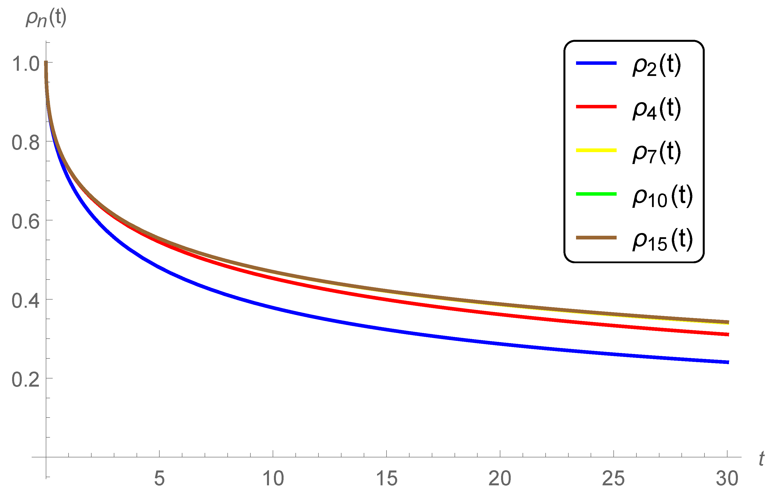
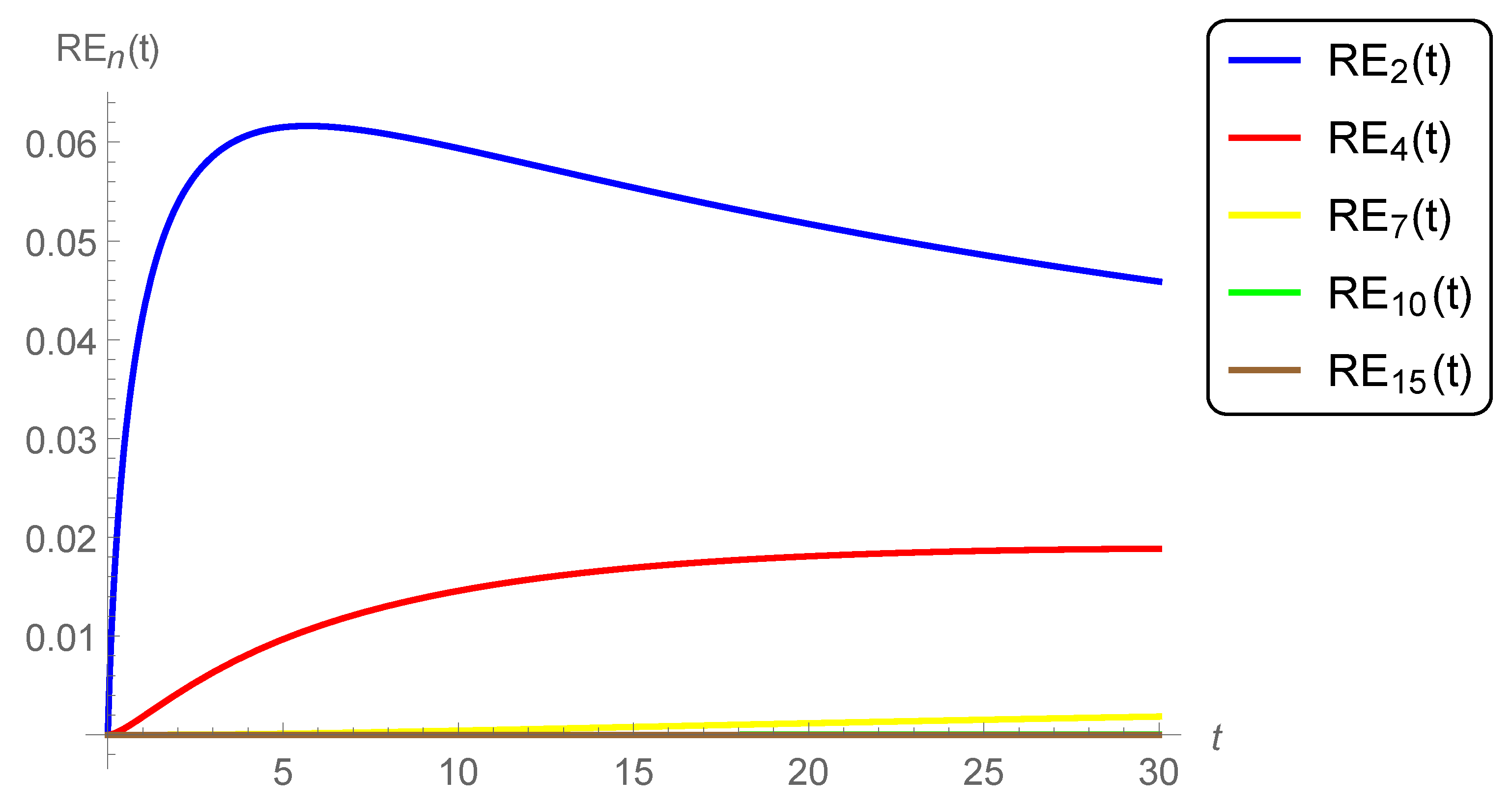
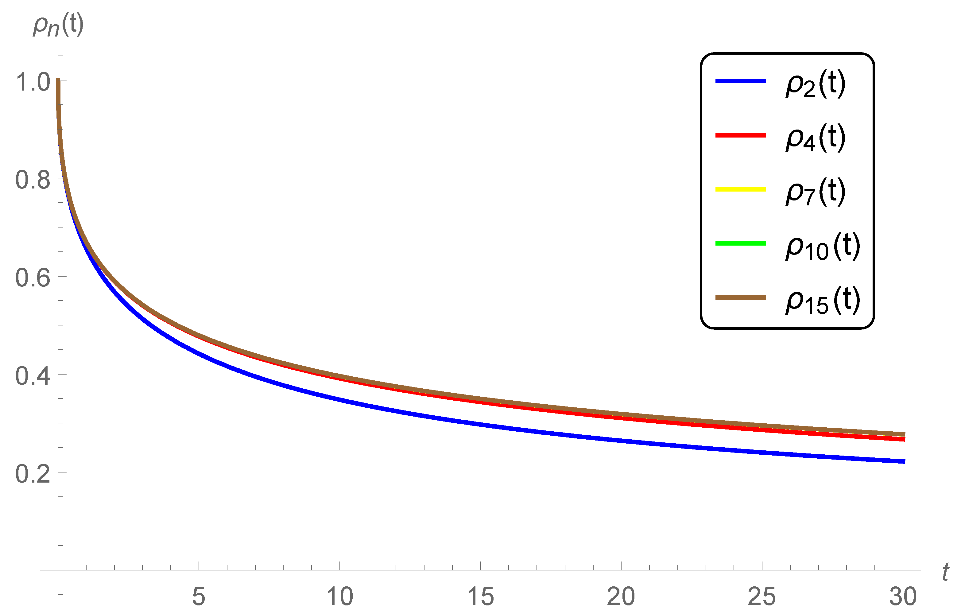
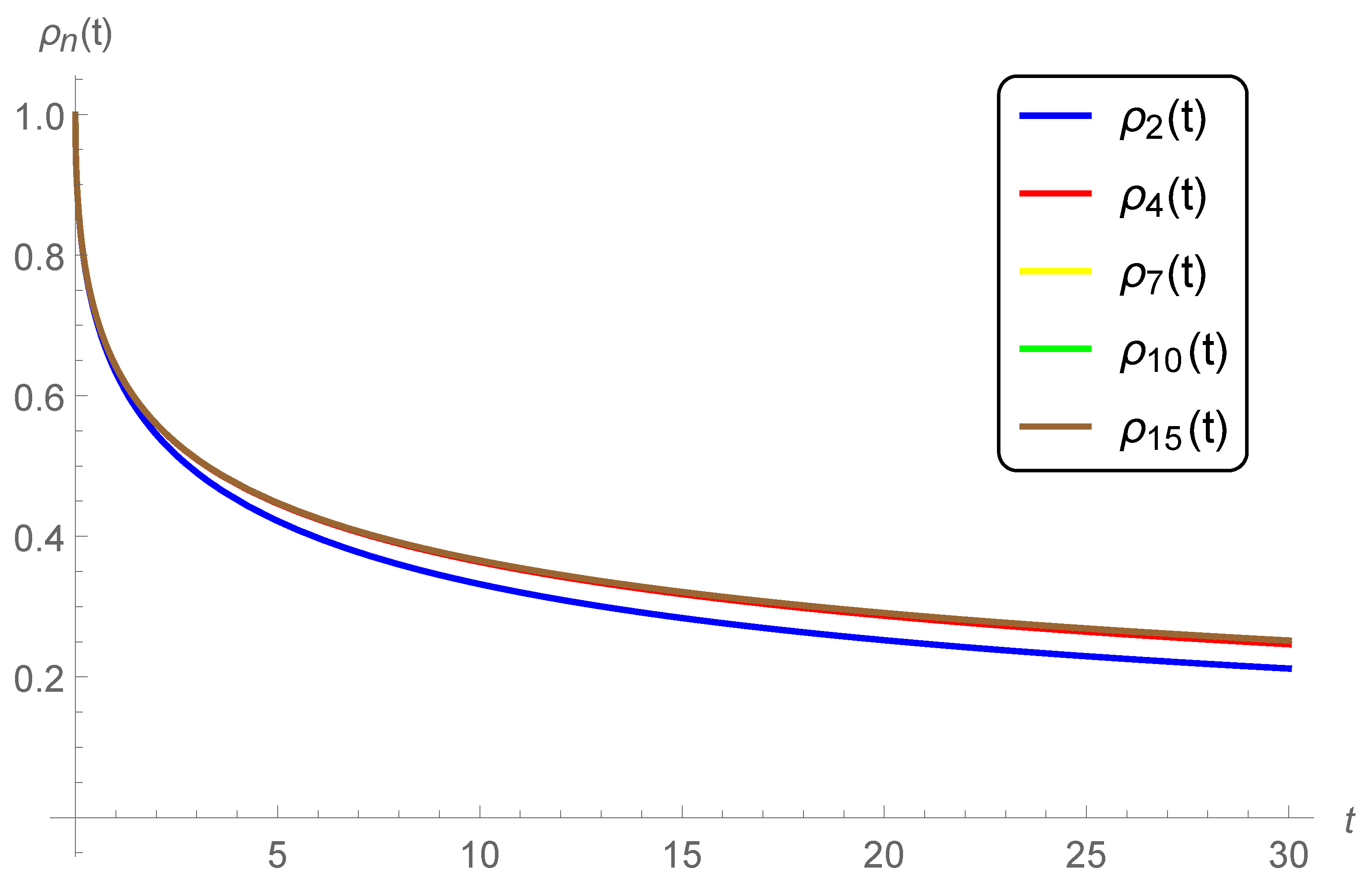
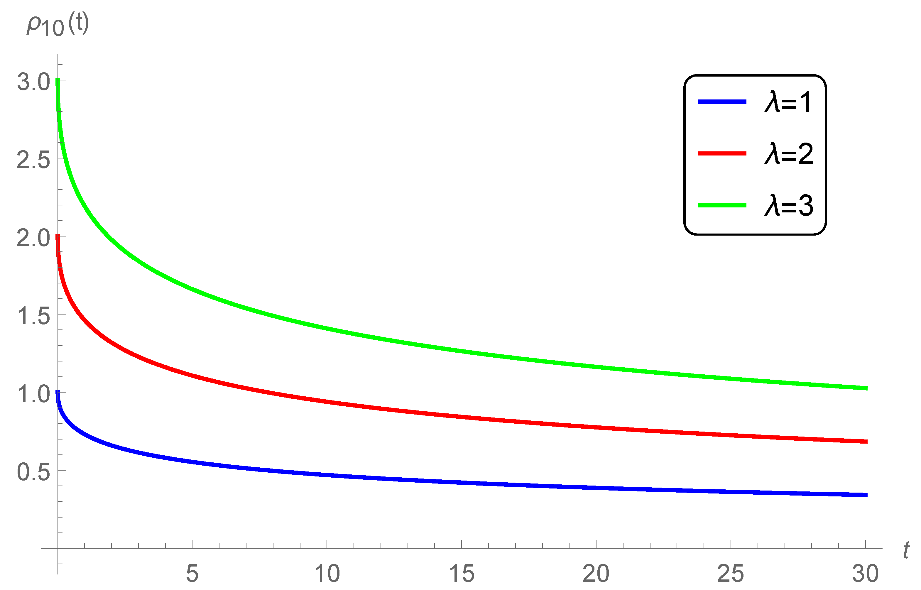
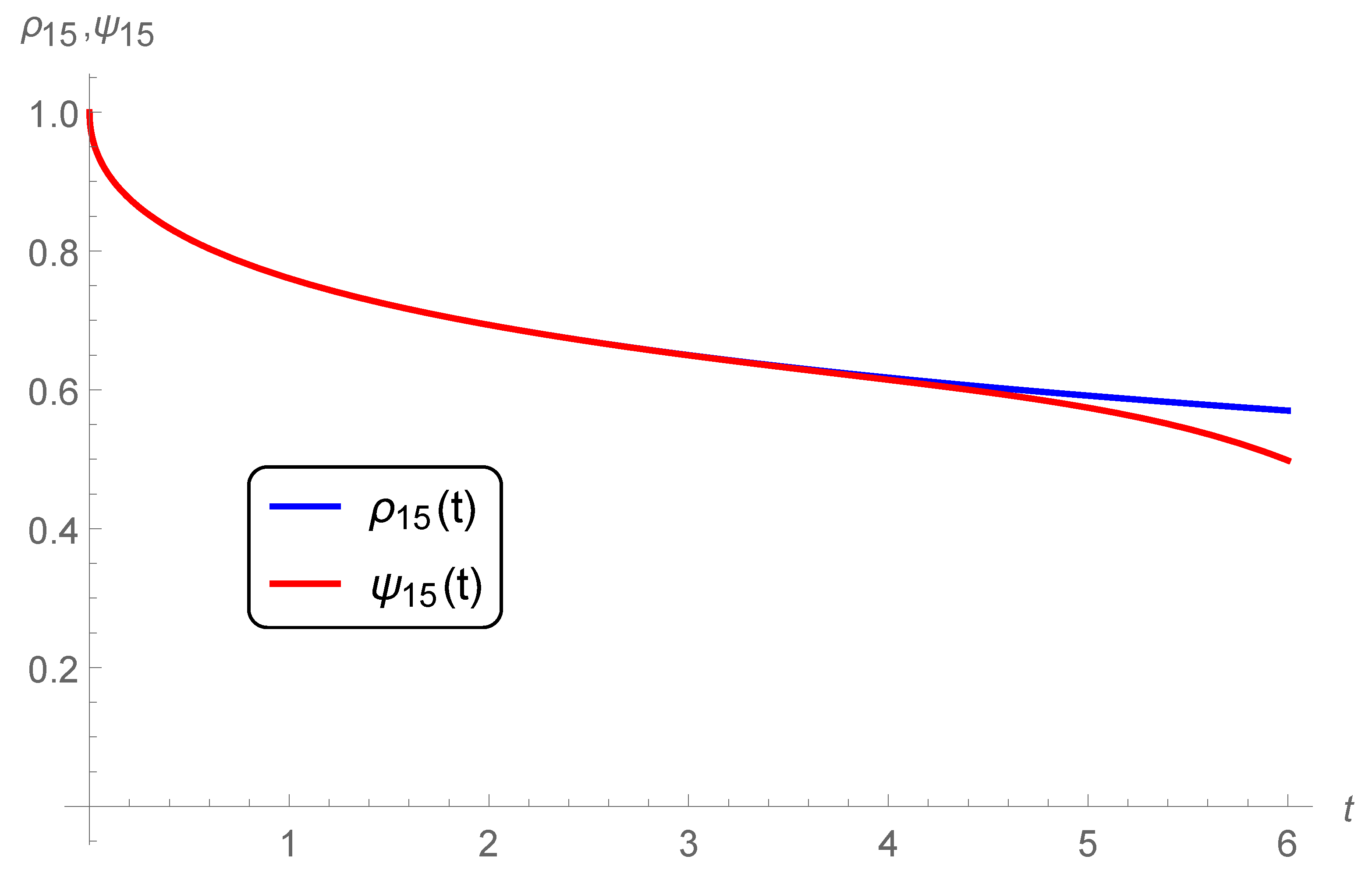
6. Numerical Simulations and Discussions

We will discuss the series solution (49) in different point of view by computer simulations. We will apply CAS Wolfram Mathematica to simulate and graph the results.

Case 1. Convergence. Consider the n-th partial sums ${\rho }_n\left(t\right)$ of the series solution (49), called n-th approximate solution of (11), (12) and the error function $R{E}_n\left(t\right)$ defined by (50) and (51), respectively. Fix $\lambda =1,q=1.5,\alpha =0.5$ and graph the partial sums (n-th approximate solution of (11), (12) ) for various values of $n=2,4,7,10,15$ (see Figure 1) and the corresponding errors (see Figure 2). In addition, the numerical results of the residual error $R{E}_{10}\left(t\right)$ at various values of $\alpha$ are tabulated in Table 1 when $q=1.5$ and Table 2 when $q=2$. From both Figures and Tables it could be seen the convergence of the n-th approximate solution of (11), (12) with increasing of n. Moreover, the obtained numerical values for the residual error $R{E}_{10}\left(t\right)$ reflects the accuracy of the present analysis.

Figure 1. Graphs of the n-th approximate solution of (11), (12) with $n=2,4,7,10,15$ and $\lambda =1$, $q=1.5$, and $\alpha =0.5$.

Figure 2. Graphs of the n-th errors $R{E}_n\left(t\right)$ with $n=2,4,7,10,15$ and $\lambda =1$, $q=1.5$, and $\alpha =0.5$.

Table 1. The residual error $R{E}_{10}\left(t\right)$ when $\lambda =1$ and $q=1.5$ at three different values of $\alpha$.

	${\mathbf{RE}}_{10}\left(\mathit{t}\right)$
$\mathbf{t}$	$\mathbf{\alpha }=\mathbf{0.5}$	$\mathbf{\alpha }=\mathbf{0.75}$	$\mathbf{\alpha }=\mathbf{1}$
0	1.8600$\times {10}^{-12}$	5.6288$\times {10}^{-14}$	1.3656$\times {10}^{-13}$
2	5.1695$\times {10}^{-9}$	3.3530$\times {10}^{-12}$	6.1451$\times {10}^{-14}$
4	7.4734$\times {10}^{-8}$	3.4129$\times {10}^{-10}$	3.0542$\times {10}^{-13}$
6	3.1829$\times {10}^{-7}$	4.4299$\times {10}^{-9}$	1.4283$\times {10}^{-11}$
8	8.3965$\times {10}^{-7}$	2.5116$\times {10}^{-8}$	1.8487$\times {10}^{-10}$
10	1.7190$\times {10}^{-7}$	9.1315$\times {10}^{-8}$	1.2649$\times {10}^{-9}$

Table 2. The residual error $R{E}_{10}\left(t\right)$ when $\lambda =1$ and $q=2$ at three different values of $\alpha$.

	${\mathbf{RE}}_{10}\left(\mathit{t}\right)$
$\mathbf{t}$	$\mathbf{\alpha }=\mathbf{0.5}$	$\mathbf{\alpha }=\mathbf{0.75}$	$\mathbf{\alpha }=\mathbf{1}$
0	1.0991$\times {10}^{-14}$	1.0603$\times {10}^{-14}$	1.9651$\times {10}^{-14}$
2	1.8281$\times {10}^{-13}$	7.2858$\times {10}^{-15}$	1.4322$\times {10}^{-14}$
4	3.7821$\times {10}^{-12}$	6.7724$\times {10}^{-15}$	1.1852$\times {10}^{-14}$
6	2.0318$\times {10}^{-11}$	9.5479$\times {10}^{-15}$	1.0519$\times {10}^{-14}$
8	6.4565$\times {10}^{-11}$	2.8588$\times {10}^{-14}$	9.8532$\times {10}^{-15}$
10	1.5476$\times {10}^{-10}$	1.0314$\times {10}^{-13}$	9.3953$\times {10}^{-15}$

Case 2. Impact of the parameter q. We fix $\lambda =1,\alpha =0.5$ and graph the n-th approximate solution of (11), (12) at $n=2,4,7,10,15$ for various values of $q=1.5$ (see Figure 1), $q=1.8$ (see Figure 3), $q=2$ (see Figure 4) and $q=2.5$ (see Figure 5). A rapid convergence is observed from these figures using only a few terms of the series solutions (49). We could see, that the rate of convergence is increased for higher values of q, for example $q>2$, where at $q=2.5$ (see Figure 5) the 4-term, 7-term, 10-term, and 15-term are nearly identical. However, a rapid decrease in the surface brightness has been remarked by increasing the delay parameter q. This latest notice reveals that the curves of the approximate solutions tend faster to zero at higher values of q.

Figure 3. Graphs of the n-th approximate solution of (11), (12) with $n=2,4,7,10,15$ and $\lambda =1$, $\alpha =0.5$, and $q=1.8$.

Figure 4. Graphs of the n-th approximate solution of (11), (12) with $n=2,4,7,10,15$ and $\lambda =1$, $\alpha =0.5$, and $q=2$.

Figure 5. Graphs of the n-th approximate solution of (11), (12) with $n=2,4,7,10,15$ and $\lambda =1$, $\alpha =0.5$, and $q=2.5$.

Case 3. Impact of the initial value λ. To study the impacts of the initial value $\lambda$ on the approximation, we fix $q=1.5,\alpha =0.5,n=10$, and graph the 10-th approximate solution ${\rho }_{10}\left(t\right)$ of (11), (12) for various values of $\lambda =1,2,3$ (see Figure 6). It can be seen from Figure 6 that the surface brightness is increased by increasing the given initial value $\lambda$.

Figure 6. Impact of the initial value $\lambda$ on the 10-term approximate solution of (11), (12) at $q=1.5$, and $\alpha =0.5$.

Case 4. Comparing the series solution (49) with known ones in the literature. The initial value problem (11), (12) is studied by some other authors and they obtained some different types of series solution. For example, in [19], the following series solution is obtained:

$$\tilde{y}\left(t\right)=\lambda \sum _{k=0}^{\infty }\frac{t^{k\alpha }}{\Gamma (k\alpha +1)}\prod _{j=1}^k\left(q^{-(k-j)\alpha -1}-1\right),$$

(58)

with n-th partial sum (n-th approximate solution of (11), (12)) defined by

$${\Psi }_n\left(t\right)=\lambda \sum _{k=0}^n\frac{t^{k\alpha }}{\Gamma (k\alpha +1)}\prod _{j=1}^k\left(q^{-(k-j)\alpha -1}-1\right).$$

(59)

We fix $\lambda =1,\alpha =0.5,q=1.4$ and graph both n-the approximate solution ${\rho }_n\left(t\right)$ and ${\Psi }_n\left(t\right)$ of (11), (12) for various values of $n=10$ (see Figure 7), $n=15$ (see Figure 8).

Figure 7. Graphs of the n-th approximate solutions ${\rho }_{10}\left(t\right)$ (present) and ${\Psi }_{10}\left(t\right)$ (Ref. [19]) for $\lambda =1$, $q=1.4$, and $\alpha =0.5$

Figure 8. Graphs of the n-th approximate solutions ${\rho }_{15}\left(t\right)$ (present) and ${\Psi }_{15}\left(t\right)$ (Ref. [19]) for $\lambda =1$, $q=1.4$, and $\alpha =0.5$

Figure 7 and Figure 8 show that both approximations coincide on an interval close to zero, however they differ for large t. However, the interval of coincidence increases by increasing the number of terms taken from both series. For example, our 10-term series solutions coincide on the interval [0, 3] (Figure 7) while taking 15-term from both series led to a coincidence on a slightly wider interval [0, 4] (Figure 8). At the same time, the approximate solutions ${\rho }_n\left(t\right),n=10,15$ are convergent to the exact solution in the whole domain of $t\ge 0$.

The numerical values of ${\rho }_{15}\left(t\right)$ (present), ${\Psi }_{15}\left(t\right)$ (Ref. [19]), and the difference $d_n\left(t\right)={\rho }_n\left(t\right)-{\Psi }_n\left(t\right)$ are tabulated in Table 3. It can be seen from this table that the difference $d_n\left(t\right)$ increases as t increases and hence $d_n\left(t\right)$ is significant. The main observation here is that the values of ${\Psi }_{15}\left(t\right)$ are negative at some points such as at $t=8$ and $t=10$ (see Table 3) which is not physically acceptable. By this, the published solution in the literature [19] is not physical in the whole domain. Therefore, our approach is applicable and convergent in the whole domain which are the main advantages of the present work over the corresponding one in the literature [19].

Table 3. Comparison between ${\rho }_{15}\left(t\right)$ (present), ${\Psi }_{15}\left(t\right)$ (Ref. [19]) when $\lambda =1$, $q=2$ and $\alpha =1$.

	${\mathit{d}}_{\mathit{n}}\left(\mathit{t}\right)={\mathit{\rho }}_{\mathit{n}}\left(\mathit{t}\right)-{\mathbf{\Psi }}_{\mathit{n}}\left(\mathit{t}\right)$
$\mathbf{t}$	${\mathbf{\rho }}_{\mathbf{15}}\left(\mathbf{t}\right)$ (Present)	${\Psi }_{\mathbf{15}}\left(\mathbf{t}\right)$ [26]	${\mathbf{d}}_{\mathbf{15}}\left(\mathbf{t}\right)$
0	1	1	0
2	0.458295	0.458159	8.1554$\times {10}^{-10}$
4	0.284022	0.283919	4.8080$\times {10}^{-5}$
6	0.204525	0.175858	2.8667$\times {10}^{-2}$
8	0.159575	−2.466450	0.2626$\times {10}^{+1}$
10	0.130763	−86.072400	0.8620$\times {10}^{+3}$

7. Conclusions

A combined approach based on the LT and the ADM was developed in this paper to solve the fractional model of the Ambartsumian delay equation with Caputo fractional derivative. The first step of such approach was applying the LT on current fractional equation and then solving the transformed equation by the ADM. It was also shown that a general formula for the $y_i\left(t\right)$-components (Adomian’s components) was successfully obtained. Hence, the exact solution was provided to the first time for fractional model of the Ambartsumian equation. Both of the approximate and the exact solutions were obtained and expressed in terms of the Mittag-Leffler functions. Moreover, the advantage of the present approach over the previous one in the relevant literature was that our solution converges in the whole domain as properties of the Mittag-Leffler functions. While the solution in the relevant literature [7] was given as a power series in terms of $t^{\alpha }$ which converges in certain domains, i.e., not valid in the whole domain of the present model. The results obtained by simulations of the studied equation reveal that the approximate solution is highly accurate. Moreover, the absolute residual error approaches zero even at higher values of the delay parameter. Finally, the authors believe that the current developed approach deserves further extensions to include and investigate other higher-order fractional delay equations.

References

1. Ambartsumian, V.A. On the Fluctuations of the Surface Brightness of Galaxies. In Plasma and the Universe; Fälthammar, C.G., Arrhenius, G., De, B.R., Herlofson, N., Mendis, D.A., Kopal, Z., Eds.; Springer: Dordrecht, The Netherlands, 1988. [Google Scholar] [CrossRef]
2. Kato, T.; McLeod, J.B. The functional-differential equation y(x)=ay(λx)+by(x). Bull. Am. Math. Soc. 1971, 77, 891–935. [Google Scholar]
3. Patade, J.; Bhalekar, S. On analytical solution of Ambartsumian equation. Natl. Acad. Sci. Lett. 2017, 40, 291–293. [Google Scholar] [CrossRef]
4. Bakodah, H.O.; Ebaid, A. Exact solution of Ambartsumian delay differential equation and comparison with Daftardar-Gejji and Jafari approximate method. Mathematics 2018, 6, 331. [Google Scholar] [CrossRef] [Green Version]
5. Alatawi, A.A.; Aljoufi, M.; Alharbi, F.M.; Ebaid, A. Investigation of the Surface Brightness Model in the Milky Way via Homotopy Perturbation Method. J. Appl. Math. Phys. 2020, 3, 434–442. [Google Scholar] [CrossRef] [Green Version]
6. Algehyne, E.A.; El-Zahar, E.R.; Alharbi, F.M.; Ebaid, A. Development of analytical solution for a generalized Ambartsumian equation. AIMS Math. 2019, 5, 249–258. [Google Scholar] [CrossRef]
7. Khaled, S.M.; El-Zahar, E.R.; Ebaid, A. Solution of Ambartsumian delay differential equation with conformable derivative. Mathematics 2019, 7, 425. [Google Scholar] [CrossRef] [Green Version]
8. Kumar, D.; Singh, J.; Baleanu, D.; Rathore, S. Analysis of a fractional model of the Ambartsumian equation. Eur. Phys. J. Plus 2018, 133, 133–259. [Google Scholar] [CrossRef]
9. Ali, E.H.; Ebaid, A.; Rach, R. Advances in the Adomian decomposition method for solving two-point nonlinear boundary value problems with Neumann boundary conditions. Comput. Math. Appl. 2012, 63, 1056–1065. [Google Scholar] [CrossRef] [Green Version]
10. Adomian, G. Solving Frontier Problems of Physics: The Decomposition Method; Kluwer Academic Publ.: Boston, MA, USA, 1994. [Google Scholar]
11. Chun, C.; Ebaid, A.; Lee, M.; Aly, E.H. An approach for solving singular two point boundary value problems: Analytical and numerical treatmen. ANZIAM J. 2012, 53, 21–43. [Google Scholar] [CrossRef] [Green Version]
12. Duan, J.-S.; Chaolu, T.; Rach, R.; Lu, L. The Adomian decomposition method with convergence acceleration techniques for nonlinear fractional differential equations. Comput. Math. Appl. 2013, 66, 728–736. [Google Scholar] [CrossRef]
13. Duan, J.S.; Rach, R. A new modification of the Adomian decomposition method for solving boundary value problems for higher order nonlinear differential equations. Appl. Math. Comput. 2011, 218, 4090–4118. [Google Scholar] [CrossRef]
14. Ebaid, A. A new analytical and numerical treatment for singular two-point boundary value problems via the Adomian decomposition method. J. Comput. Appl. Math. 2011, 235, 1914–1924. [Google Scholar] [CrossRef] [Green Version]
15. Ebaid, A.; Al-Enazi, A.; Albalawi, B.Z.; Aljoufi, M.D. Accurate Approximate Solution of Ambartsumian Delay Differential Equationation via Decomposition Method. Math. Comput. Appl. 2019, 24, 7. [Google Scholar]
16. Rach, R. A bibliography of the theory and applications of the Adomian decomposition method, 1961–2011. Kybernetes 2012, 41, 1087–1148. [Google Scholar] [CrossRef]
17. Jafari, H.; Daftardar-Gejji, V. Solving a system of nonlinear fractional differential equations using Adomian decomposition. J. Comput. Appl. Math. 2006, 196, 644–651. [Google Scholar] [CrossRef] [Green Version]
18. Junsheng, D.; Jianye, A.; Mingyu, X. Solutions of systems of fractional differential equations by Adomian decomposition method. Appl. Math. J. Chin. Univ. Ser. B 2007, 22, 7–12. [Google Scholar]
19. Shah, R.; Khan, H.; Arif, M.; Kumam, P. Application of Laplace-Adomian decomposition method for the analytical solution of third-order dispersive fractional partial differential equations. Entropy 2019, 21, 335. [Google Scholar] [CrossRef] [PubMed] [Green Version]
20. Wazwaz, A.M. The combined Laplace transform-Adomian decomposition method for handling nonlinear Volterra integro-differential equations. Appl. Math. Comput. 2010, 216, 1304–1309. [Google Scholar] [CrossRef]
21. Wazwaz, A.M.; Rach, R.; Duan, J.S. Adomian decomposition method for solving the Volterra integral form of the Lane-Emden equations with initial values and boundary conditions. Appl. Math. Comput. 2013, 219, 5004–5019. [Google Scholar] [CrossRef]
22. Fatoorehchi, H.; Rach, R. A method for inverting the Laplace transforms of two classes of rational transfer functions in control engineering. Alexandria Eng. J. 2020. [Google Scholar] [CrossRef]
23. Alharbi, W.; Petrovskii, S. Numerical Analysis for the Fractional Ambartsumian Equation via the Homotopy Herturbation Method. Mathematics 2020, 8, 2247. [Google Scholar] [CrossRef]
24. Podlubny, I. Fractional Differential Equationations; Academic Press: San Diego, CA, USA, 1999. [Google Scholar]
25. Spiegel, M.R. Laplac Transforms; McGraw-Hill Inc.: New York, NY, USA, 1965. [Google Scholar]
26. Patade, J. Series solution of system of fractional order Ambartsumian equations: Application in Astronomy. arXiv 2020, arXiv:2008.04904v1. [Google Scholar]