A New Derivative-Free Method to Solve Nonlinear Equations

Abstract

A new high-order derivative-free method for the solution of a nonlinear equation is developed. The novelty is the use of Traub’s method as a first step. The order is proven and demonstrated. It is also shown that the method has much fewer divergent points and runs faster than an optimal eighth-order derivative-free method.

1. Introduction

In engineering and applied science, we encounter the problem of solving a nonlinear equation

$$f\left(x\right)=0$$

(1)

For example, the Colebrook equation [1] to find the friction factor, or finding critical values of some nonlinear function. Another example is given by Ricceri [2] where the first eigenvalue of Helmholtz equation is found by minimizing a functional. See also [3]. Most numerical solution methods are based on Newton’s scheme, i.e., starting with an initial guess $x_0$ for the root $\xi$, we create a sequence $\left\{x_n\right\}$

$$x_{n+1}=x_n-\frac{f\left(x_n\right)}{f^{\prime }\left(x_n\right)}.$$

(2)

The convergence is quadratic, that is,

$$|x_{n+1}-\xi |\le C_2{|x_n-\xi |}^2.$$

(3)

To increase the order, one has to include higher derivatives, such as Halley’s scheme [4] using first and second derivatives and is of a cubic order. In order to avoid higher derivatives, one can use multipoint methods, see Petković et al. [5].

Derivative-free methods are either linear (such as Picard), super-linear (such as secant) or even quadratic, such as Steffensen’s method [6], given by

$$\begin{array}{c}{\displaystyle w_n=x_n+\gamma \left(f\left(x_n\right)\right)}\hfill \\ {\displaystyle x_{n+1}=x_n-\frac{\gamma {\left(f\left(x_n\right)\right)}^2}{f(w_n-f\left(x_n\right))}}\hfill \end{array}$$

(4)

Because multistep methods are usually based on Newton’s steps, derivative-free methods are based on Steffensen’s method as the first step. There are several derivative-free methods based on Steffensen’s method for simple and multiple roots. See Kansal et al. [7] for such family of methods for multiple roots and Zhanlav and otgondorj [8] for simple roots. In a recent article, Neta [9] has shown that there is a better choice for a first step, even though it is NOT second order. Traub’s method [10], given by

$${\displaystyle x_{n+1}=x_n-\frac{f\left(x_n\right)}{{\displaystyle \frac{(f\left(x_{n-2}\right)--f\left(x_n\right))}{(x_{n-2}-x_n)}-\frac{f\left(x_{n-2}\right)-f\left(x_{n-1}\right)}{x_{n-2}-x_{n-1}}+\frac{f\left(x_{n-1}\right)-f\left(x_n\right)}{x_{n-1}-x_n}}}}$$

(5)

is of order 1.839, and it runs faster and has better dynamics than several other derivative-free methods. Clearly, one cannot get optimal methods (see Kung and Traub [11]) this way. Kung and Traub [11] conjectured that multipoint methods without memory using d function evaluations could have an order no larger than $2^{d-1}$. The efficiency index I is defined as $p^{1/d}$. Thus, an optimal method of order 8 has an efficiency index of $I=8^{1/4}=1.6817$ and an optimal method of order 4 has an efficiency index $I=4^{1/3}=1.5874$, which is better than Newton’s method for which $I=\sqrt{2}=1.4142$. The efficiency index of optimal method cannot reach a value of 2. In fact, realistically, one uses methods of an order of at most 8. For high order derivative-free methods based on Steffensen’s method as a first step, see Zhanlav and Otgondorj [8] and references there. Such methods are especially useful when the derivative is very expensive to evaluate and, of course, when the function is non-differentiable.

Here, we develop a derivative-free method with memory based on Traub’s method (5) as the first step and the other two steps are based on replacing the derivative by the derivative of Newton interpolating polynomial of degree 3. In the next section, we will discuss the order of the scheme and the computational order of convergence, COC, defined by

$${\displaystyle coc=\frac{{\displaystyle ln\left|\frac{x_i-\alpha }{x_{i-1}-\alpha }\right|}}{{\displaystyle ln\left|\frac{x_{i-1}-\alpha }{x_{i-2}-\alpha }\right|}}}$$

(6)

where $\alpha$ is the final approximation for the zero $\xi$.

2. New Method

We suggest a 3-step method having (5) as the first step. The method is

$$\begin{array}{c}{\displaystyle y_n=x_n-\frac{f\left(x_n\right)}{{\displaystyle \frac{(f\left(x_{n-2}\right)-f\left(x_n\right))}{(x_{n-2}-x_n)}-\frac{f\left(x_{n-2}\right)-f\left(x_{n-1}\right)}{x_{n-2}-x_{n-1}}+\frac{f\left(x_{n-1}\right)-f\left(x_n\right)}{x_{n-1}-x_n}}},}\hfill \\ \\ {\displaystyle z_n=y_n-\frac{f\left(y_n\right)}{f^{\prime }\left(y_n\right)},}\hfill \\ \\ {\displaystyle x_{n+1}=z_n-\frac{f\left(z_n\right)}{f^{\prime }\left(z_n\right)}.}\hfill \end{array}$$

(7)

The derivatives in the last two steps are approximated by the derivative of Newton interpolating polynomial of degree 3:

$$f^{\prime }\left(y_n\right)=f[y_n,x_n]+f[y_n,x_n,x_{n-1}](y_n-x_n)+f[y_n,x_n,x_{n-1},x_{n-2}](y_n-x_n)(y_n-x_{n-1}),$$

(8)

and

$$f^{\prime }\left(z_n\right)=f[z_n,y_n]+f[z_n,y_n,x_n](z_n-y_n)+f[z_n,y_n,x_n,x_{n-1}](z_n-y_n)(z_n-x_n),$$

(9)

and $f[a,b]$ is the divided difference.

Let us denote the errors $e_n=x_n-\xi$, $e_y=y_n-\xi$ and $e_z=z_n-\xi$. The error in the first step is given by Traub

$$e_y=C{e}_n^{1.839}.$$

The other two steps are of the same order as the Newton’s method, i.e., $e_z=e_y^2$ and $e_{n+1}=e_z^2.$ Therefore, the order of the method is $4\times 1.839=7.356.$ The efficiency index ${\displaystyle I=p^{1/d}=7.{356}^{1/3}=1.945}$ is higher than that of the 3-step optimal eighth order method. This is typical of methods with memory.

In

Table 1. Computational order of convergence for several functions using our new method.

Index	$\mathit{f}\left(\mathit{x}\right)$	${\mathit{x}}_0$	Number of Iterations	COC
1	$\left(e^{x+3}-1\right)(x-1)$	10.0	8	6.78
2	$x^3+4x^2-10$	−2.6	30	7.048
3	${(sinx)}^2-x^2+1$	2.0	3	6.622
4	${(x-1)}^3-1$	3.5	4	6.728
5	$x^3-10$	4.0	4	6.901
6	$x{e}^{x^2}-{(sinx)}^2+3cosx+5$	−1.0	3	7.048
7	$e^{x^2+7x-30}-1$	4.0	9	6.793
8	$sinx-x/2$	2.0	3	6.848
9	$x^5+x-10,000$	4.0	4	6.780
10	$\sqrt{(}x)-1/x-3$	9.0	3	6.674
11	$e^x+x-20$	0.0	5	7.049
12	$lnx+\sqrt{(}x)-5$	10.0	3	6.659
13	$x^3-x^2-1$	4.0	4	6.912
14	$x^5-1$	10.0	7	6.749
15	$\left(e^{x+1}-1\right)(x-1)$	5.0	5	7.394
16	$\left(e^{x+3}-1\right)\left(e^{x-1}-1\right)$	15.0	14	6.964

, we list the computational order of convergence as defined by (6) for 16 different nonlinear functions. The values range from 6.622 to 7.394 with an average value of 6.872.

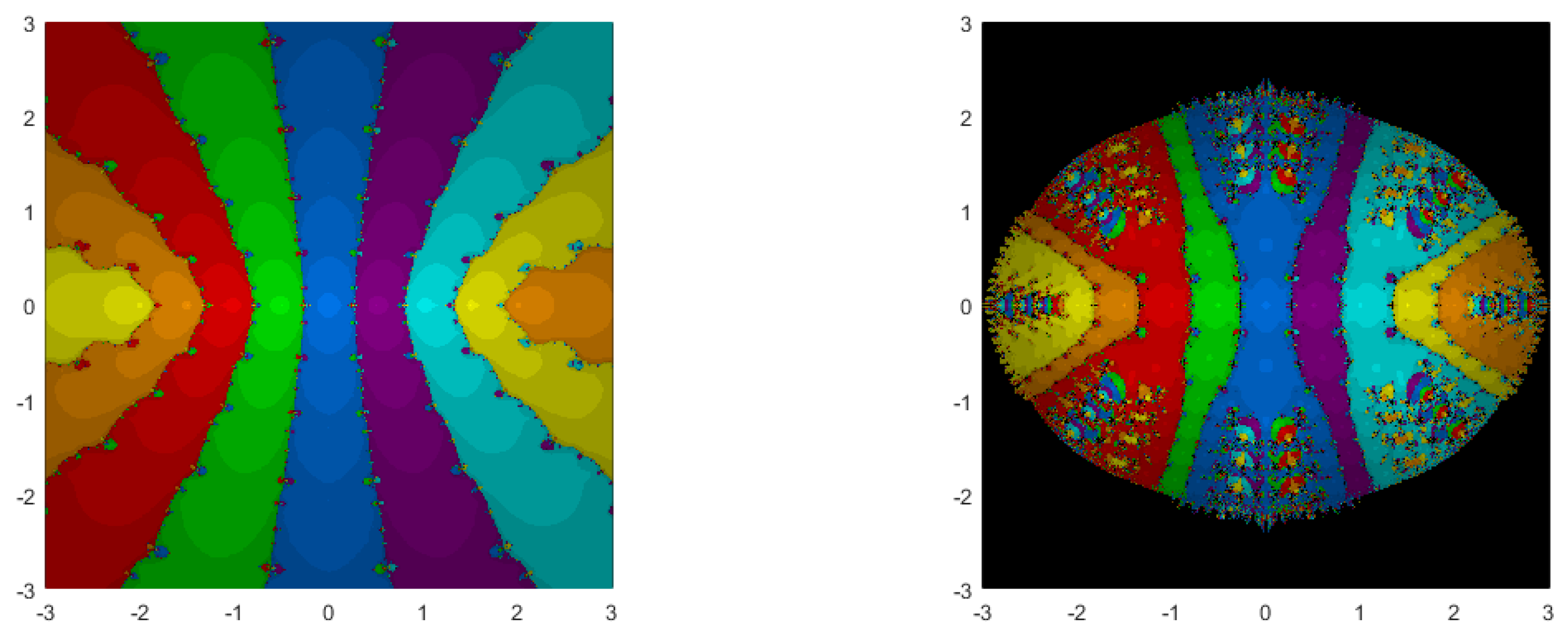
3. Dynamics Study of the Methods

The basin of attraction method was initially discussed by Stewart [12]. This is better than comparing methods on the basis of running several nonlinear functions using a certain initial value. In the last decade, many papers appeared using the idea of basin of attraction to compare the efficiency of many methods. See, for example, Chun and Neta [13,14] and references there.

In this section, we describe the experiments with our method as compared to TZKO [8].

We chose four polynomials and one non-polynomial function all having roots within a 6 by 6 square centered at the origin. The square is divided horizontally and vertically by equally spaced lines. We took the intersection of all these lines as initial points in the complex plane for the iterative schemes. The code collected the number of iteration or function evaluation to converge within a tolerance of ${10}^{-7}$ and the root to which the sequence converged. If the sequence did not converge within 40 iterations, we denote it as a divergent point. We also collected the CPU run time to execute the code on all initial points using a Dell Optiplex 990 desktop computer.

We ran all methods on the following five examples, four of which are polynomials:

• $z^2-1$
• $z^3-1$
• $z^4-1$
• $z^5-1$
• $\left(e^{z+1}-1\right)(z-1)$

Remark 1.

The additional starting values are $x_{-1}=x_0+0.01$ and $x_{-2}=x_0+0.02$.

It is clear from these tables that our method runs faster (see

Table 2. CPU time (msec) for each example (1–5) and each of the methods.

Method	Ex1	Ex2	Ex3	Ex4	Ex5	Average
TZKO	290.886	545.869	621.265	745.541	334.541	507.620
Neta	201.156	277.703	391.063	435.844	302.438	321.641

), uses fewer function-evaluations per point (see

Table 3. Average number of function evaluations per point for each example (1–5) and each of the methods.

Method	Ex1	Ex2	Ex3	Ex4	Ex5	Average
TZKO	11.85	19.52	25.60	29.26	12.25	19.70
Neta	6.77	8.01	10.72	11.02	8.37	8.98

) and has much fewer divergent points (see

Table 4. Number of black points for each example (1–5) and each of the methods.

Method	Ex1	Ex2	Ex3	Ex4	Ex5	Average
TZKO	2364	16,674	27,745	33,419	2640	16,568
Neta	487	0	0	0	2542	606

). In fact, for 3 out of 5 examples, our method had NO divergent points. We now take an example known to be hard, i.e., the Wilkinson-type polynomial

$$q\left(z\right)=z(z^2-1/4)(z^2-1)(z^2-9/4)(z^2-4)$$

(10)

which has roots at $z=0,\pm 1/2,\pm 1,\pm 3/2,\pm 2.$ Our method runs fast and had no divergent points. TZKO requires more than double the CPU run time for our method and had 166,138 divergent points. The plots of the basins for this example are given in Figure 1.

4. Conclusions

We have developed a derivative-free method with memory based on Traub’s method as the first step. The method is of order 7.356 and has an efficiency index of 1.945, which is higher than any optimal eighth order method. We have shown that our method is faster, uses fewer function evaluations per point, and has much fewer divergent points.

References

1. Colebrook, C.F. Turbulent flows in pipes, with particular reference to the transition between the smooth and rough pipe laws. J. Inst. Civ. Eng. 1939, 11, 130. [Google Scholar] [CrossRef]
2. Ricceri, B. A class of equations with three solutions. Mathematics 2020, 8, 478. [Google Scholar] [CrossRef] [Green Version]
3. Treantă, S. Gradient structures associated with a polynomial differential equation. Mathematics 2020, 8, 535. [Google Scholar] [CrossRef] [Green Version]
4. Halley, E. A new, exact and easy method of finding the roots of equations generally and that without any previous reduction. Philos. Trans. R. Soc. Lond. 1694, 18, 136–148. [Google Scholar]
5. Petković, M.S.; Neta, B.; Petković, L.D.; Džunić, J. Multipoint Methods for the Solution of Nonlinear Equations; Elsevier: Amsterdam, The Netherlands, 2012. [Google Scholar]
6. Steffensen, J.F. Remarks on iteration. Scand. Actuar. J. 1933, 1, 64–72. [Google Scholar] [CrossRef]
7. Kansal, M.; Alshomrani, A.S.; Bhalla, S.; Behl, R.; Salimi, M. One parameter optimal derivative-free family to find the multiple roots of algebraic nonlinear equations. Mathematics 2020, 8, 2223. [Google Scholar] [CrossRef]
8. Zhanlav, T.; Otgondorj, K. Comparison of some optimal derivative-free three-point iterations. J. Numer. Anal. Approx. Theory 2020, 49, 76–90. [Google Scholar]
9. Neta, B. Basin attractors for derivative-free methods to find simple roots of nonlinear equations. J. Numer. Anal. Approx. Theory 2020, 49, 177–189. [Google Scholar]
10. Traub, J.F. Iterative Methods for the Solution of Equations; Prentice Hall: New York, NY, USA, 1964. [Google Scholar]
11. Kung, H.T.; Traub, J.F. Optimal order of one-point and multipoint iteration. J. Assoc. Comput. Math. 1974, 21, 634–651. [Google Scholar] [CrossRef]
12. Stewart, B.D. Attractor Basins of Various Root-Finding Methods. Master’s Thesis, Naval Postgraduate School, Department of Applied Mathematics, Monterey, CA, USA, June 2001. [Google Scholar]
13. Chun, C.; Neta, B. Comparative study of methods of various orders for finding simple roots of nonlinear equations. J. Appl. Anal. Comput. 2019, 9, 400–427. [Google Scholar] [CrossRef]
14. Chun, C.; Neta, B. Comparative study of methods of various orders for finding repeated roots of nonlinear equations. J. Comput. Appl. Math. 2018, 340, 11–42. [Google Scholar] [CrossRef]
Figure 1. Our method (left) and TZKO (right) for the roots of the polynomial q ( z ) (10).
Mathematics 09 00583 g001