Abstract
A straightforward family of one-point multiple-root iterative methods is introduced. The family is generated using the technique of weight functions. The order of convergence of the family is determined in its convergence analysis, which shows the constraints that the weight function must satisfy to achieve order three. In this sense, a family of iterative methods can be obtained with a suitable design of the weight function. That is, an iterative algorithm that depends on one or more parameters is designed. This family of iterative methods, starting with proper initial estimations, generates a sequence of approximations to the solution of a problem. A dynamical analysis is also included in the manuscript to study the long-term behavior of the family depending on the parameter value and the initial guess considered. This analysis reveals the good properties of the family for a wide range of values of the parameter. In addition, a numerical test on academic and engineering multiple-root functions is performed.
1. Introduction
Solving nonlinear equation has been a difficult problem to handle for a long time in several branches of Science and Engineering. Although Newton’s method dates from the 17th century, it is at the end of the 20th century that computing drives research in the discipline of iterative methods. Hundreds of papers can be found covering this topic in the most recent literature.
An initial classification splits the problem in methods without or with memory for single or multiple roots. The variety of publications is vast. Furthermore, the stability of the iterative procedures is also analyzed in several publications. Focusing on methods without memory, we can find complete analysis for single-root finding on simple two-step methods [1,2,3,4,5], as well as those that reach orders of convergence of value 16 [6,7,8,9] most of them collected in [10]. In a similar manner, multiple-root finding procedures—recently very aptly named as root-ratio methods [11]—are also present in the literature with a large variety of orders of convergence (see [12,13] and the references therein). In this sense, the higher order of convergence, the higher computational cost.
Iterative methods for finding single roots of a nonlinear equation often lose their order of convergence when used for multiple roots. A classic example is Newton’s method, with quadratic order of convergence for single roots, but it has linear convergence when it is applied for finding multiple roots. However, several modifications have been proposed in order to keep its quadratic order. Among them, we find Newton’s accelerated method (or Rall’s method [14]) and the modified Newton’s scheme (or Schröder’s method [15]), based on applying Newton’s iterative scheme to the functions and , respectively. In both cases, the problem becomes finding a simple root of a nonlinear equation, so the order of convergence is again quadratic.
Linear combinations of these two previous methods can also generate schemes that hold the order of convergence two. Mora [16] proposes a one-parametric family. In particular, the method of the family obtained when is the well-known SuperHalley’s method that has order of convergence three.
In this paper we focus on a simple idea for generating a class of one-step iterative methods for finding multiple roots of nonlinear equations. A specific case of weight function is developed, including a parameter, and therefore a family of iterative methods is generated. In order to select the most stable methods of the family, a dynamical study is carried out. To this end, we perform a complex dynamics analysis, in which fixed and critical points—and their asymptotic behavior—allows the knowledge of the stability of the family. As a consequence, we will be able to select the members of the family whose basins of attraction are wider, ensuring the convergence of the method for a wide set of initial estimates. This analysis is more common for single root methods; however, there are papers that include it for multiple root methods [17,18,19,20,21].
This paper is organized as follows. In Section 2 we present the iterative one-step family based on a weight function, as well as its convergence analysis. The stability analysis of the family is performed in Section 3, where we find that compliance with the Scaling Theorem simplifies the study. Section 4 covers the numerical analysis for specific members of the family on different nonlinear functions with multiple roots. Finally, Section 5 collects the main conclusions.
2. Convergence Analysis of the Parametric Family
Mora [16] introduced the one-parameter family
Family (1) can also be written as
Following this guideline and in order to design iterative schemes of order three for multiple roots, we propose the following triparametric family
where the weight function and its variable are given by
Theorem 1 shows the conditions that the parameters and must satisfy for the family to reach the order of convergence three. The proof of the theorem is based on Taylor series developments around the solution since the initial estimates are taken close to the solution. The only requirement for the function is to be sufficiently differentiable.
Theorem 1.
Let us consider a multiple root with multiplicity of a sufficiently differentiable function defined in an open interval I. If the initial estimation is close enough to r, then iterative family (3) has order of convergence 3 when parameters satisfy
In addition, its error equation is given by
where , , and denotes the error in each iteration.
Proof.
Considering the Taylor series expansions of , and around r and taking into account that , and , we have
being
Using Equation (5) and developing the weight function variable , we obtain
where the coefficients , , are given by
In order to achieve order of convergence 3, we must solve equations and . Then, we obtain the values for parameters and :
After some algebraic manipulations, (8) can be written as a Chebyshev-Halley type expression:
Let us note that gives Chebyshev-Halley’s family of iterative schemes for simple roots
From now on, we consider the third-order iterative family resulting after applying the previous conditions. This parametric family can be expressed as follows:
Family Equation (10) collects all Chebyshev-Halley’s methods for single or multiple roots and only these. Some of the well-known methods of this family can be deduced from different values of :
- Chebyshev ():
- Halley ():
- Super-Halley ():
- Osada ():
3. Dynamical Analysis of the Family
In this section, we conduct a dynamical analysis of the iterative family under study trough complex dynamics. After a review of the basics on complex dynamics, we apply the scaling theorem. The rational function after Möbius conjugation gives us an expression from which the fixed and critical points are obtained. Finally, some well-known representations–such as the stability, the parameters or the dynamical plane–provides us with important information about the stability of the family.
First, the fundamental tools needed to begin this complex dynamics study are described in Section 3.1. This dynamical tools are defined for a rational function, which is obtained later after applying the corresponding iterative method on a polynomial.
3.1. Preliminaries on Complex Dynamics
In this part, the basics of the complex dynamics are revisited. For a more extensive explanation, see [22,23,24].
Let be a rational function, where is the Riemann sphere. The orbit of a point is the set consisting of the successive applications of Q on the point , i.e.,
A point that remains unaltered with the application of Q is a fixed point, that satisfies . The asymptotic behavior of the fixed points sorts them into attracting, repelling, neutral or superattracting, depending on the value of the multiplier . Table 1 gathers the conditions for classifying a fixed point inside one of the above-mentioned groups.

Table 1.
Classification of fixed points.
The evaluation of the infinity as a fixed point and its asymptotic behavior can be obtained with the technique presented in [25] and widely applied ([26] or [27], among others).
When the rational function is the result of the application of a function on an iterative method, the fixed points match with the roots of f. In addition, more fixed points may appear, which are called strange fixed points. The presence of these additional points may alter the stability of the iterative method, as long as its asymptotic behavior is not repelling.
A critical point is a point that satisfies . Again, the roots of f match with the critical points, and the additional points that do not match are named free critical points.
Finally, the basin of attraction of an attracting fixed point is the set of initial estimations whose orbit converge to this attracting fixed point, i.e.,
When the iterative expression includes a parameter, it is worth mentioning the associated graphic tools [28]. On the one hand, the unified stability plane gathers in one representation the regions of the parameter where the strange fixed points behave as attracting points, altering the stability of the method. On the other hand, the unified parameter plane represents the regions of the parameter where the free critical points converge either to a root of the function f or to another point.
3.2. The Rational Function
In the following, we are going to analyze the stability of family (10) on cubic polynomials with double roots. We will use for this study the generic polynomial , . Previously, we will apply the Scaling Theorem in order to simplify this study.
For this purpose, let us recall the fixed point operator obtained when family (10) is applied to an analytical function in :
where .
Theorem 2
Proof.
First, let us consider the following equalities:
- ,
- ,
- .
Then we have
and
The Scaling Theorem (Theorem 2) proves that the fixed point operators associated to family (10) applied to different analytic functions are affine conjugated by an affine map. Thus, the dynamical study of the roots of a cubic polynomial with a double root can be reduced by an affine change of coordinates to the dynamics associated with the generic cubic polynomial .
The rational operator obtained when family (10) is applied on is
which depends not only on but also on parameters a and b.
In order to work with a rational operator with dependence only on a parameter, we apply Möbius transformation
and we obtain a rational operator that only depends on parameter
Fixed point operator is affine conjugated to by M, so the study of the dynamics is equivalent.
Since , and , Möbius transformation has sent the roots a and b to 0 and ∞, respectively, while the divergence is set in 1. Now the fixed points of are 0 and ∞, which correspond to the roots of with multiplicity 2 and 1, respectively.
In order to study the asymptotic behavior of the fixed points and to obtain the critical points of the rational operator, we consider its derivative, whose expression is
However, the study of the fixed point ∞ requires a different analysis [25]. The point ∞ is a fixed point of if, and only if, is a fixed point of the function . In addition, ∞ is classified as attracting when , repelling if and neutral when . In this analysis, rational functions and are given by
For all value of it is satisfied and , so the roots and are fixed points of the fixed point operator.
Now, we analyze the set of strange fixed points and free critical points of and also the asymptotic behavior of the fixed points.
Lemma 1.
The fixed point operator has the following three strange fixed points
when .
Proof.
Solving the equation , we obtain the strange fixed points , and .
On the one hand, the values are roots of , so they cancel the numerator of and . On the other hand, and are roots of . In addition, is solution of the equations and . Then, we consider this set of values of and the associated fixed point operator is analyzed for each case.
- When , we getThe solutions of are , and , so the rational operator has two strange fixed points.
- If ,and is the only strange fixed point.
- When , turns intoThe points , and are the solutions of . Then, there exist two strange fixed points.
- If , the fixed point operator isThe only strange fixed point for this case is . □
From (20), solving equation we obtain the critical points as shown the following result.
Lemma 2.
The critical points of the fixed point operator are , corresponding to the double root of the polynomial, and four free critical points, corresponding to the roots of polynomial
In particular, when there is only a free critical point, for there exist two different free critical points, and if , the fixed point operator has three free critical points.
3.3. Asymptotic Behavior of Fixed and Critical Points
In order to design iterative schemes with stability depending on the initial estimations, it is desirable that the strange fixed points are repelling, so the iterative process does not converge to points different to the roots of the function.
According to Lemma 1, rational operator has strange fixed points, so we must study its asymptotic behavior to determine the values of parameter that correspond to the methods of the family with the best dynamic properties.
Lemma 3.
Fixed point is superattracting for all value of α. Fixed point is attracting when , neutral if , and repelling when .
Proof.
On the one hand, from (20) we have , so is a superattracting fixed point.
On the other hand, from (22), . Then, is:
- Attracting if , that is, when (and superattracting when ).
- Neutral when , so .
- Repelling if , and then . □
Lemma 4.
The strange fixed point of the rational function is attracting inside the disk
where and denote the real and imaginary parts of α, respectively; repelling outside the disk; neutral when , and superattracting if .
Proof.
From (20), we get
Then, is:
- Attracting if .
- Neutral if .
- Repelling: when .
- Superattracting if , that is when .
Developing , we get , which corresponds to the circumference . Then, we obtain the above results. □
The asymptotic behavior of the strange fixed points and is set through the derivatives
However, the resulting expressions make difficult the analytical study. Instead of it, we represent the stability regions in the complex plane for each strange fixed point depending on the value of .
Figure 1 and Figure 2 represent the stability planes associated to the strange fixed points and , respectively. The real part of is represented in the abscissas axis and the imaginary part of is represented in the ordinate axis. White regions represent the values of where the strange fixed point is attracting, while blue color represents the values of the parameter where the strange fixed point is repelling. The borders between the regions are the values where the strange fixed point is neutral.

Figure 1.
Stability plane of for .

Figure 2.
Stability plane of .
In addition, Figure 2 shows the value of in the complex plane where the strange fixed points and behave as attracting points. Let us remark that Figure 3b is a detail of the red region represented in Figure 3a where the root is attracting.

Figure 3.
Asymptotic behavior of the strange fixed points of and .
According to Figure 3a, the only attracting point outside the green and red regions is the double root . In order to choose the methods of the family with the best properties in terms of stability, we must avoid the areas represented with any color other than white in Figure 3b.
In a family of iterative schemes with dependence on a parameter, the parameters plane provides an overview of the stability of the family. In this paper, parameters planes are generated using a mesh of points in the complex plane, where the real and imaginary part of parameter are represented in the abscissas and ordinate axis, respectively. Each point in the plane corresponds to a value of , that is, with a method of the iterative family. Taking a free critical point as initial estimation to iterate each method associated to a value of , the point is represented in red when there is convergence to any root of the polynomial and otherwise, the point is plotted in black. Therefore, there exist points in the black regions, different to the roots 0 and ∞, that behave as attracting points. These points can be strange fixed points or attracting periodic points. Then, the most stable methods of the family are located in the plane in the red regions.
According to Lemma 2, rational operator has four free critical points. We can see in Figure 4 the parameters plane associated to each free critical point for . They have been generated using Matlab and the implementation presented in [29]. The iterative process finishes when the difference between the point and some of the roots is lower than with a maximum of 150 iterations.

Figure 4.
Parameters plane.
Figure 4 shows wide red areas for the four free critical points. This areas allow us to select values of parameter where the associated scheme converges to a root taking as initial iterate a free critical point. In addition, we have choose from Figure 4 different values of to generate the corresponding dynamical planes and then compare the stability of methods that belong to the same family.
The dynamical planes show the basins of attraction of an attracting point. Each point in the complex plane is taken as initial estimation to iterate the method and, according to the root to which its orbit converges, it is represented with a color. In this paper, the dynamical planes have been generated in Matlab according to [29]. A mesh of points in the complex plane are taken as initial estimations, being the stopping criteria a maximum of 50 iterations or a difference between the point and an attracting point lower than .
We have denoted the basins of attraction of and in orange or green, respectively. Moreover, colors blue and red denote the convergence to a strange fixed point. Finally, the point in the plane is depicted in black when its orbit is divergent or converges to any other attracting point different to the roots or the strange fixed points. Moreover, colors are lighter when less iterations are required until the convergence.
Figure 5 and Figure 6 show the dynamical planes associated to values of where the number of strange fixed points is lower than three (Lemma 1), that is . In all the cases the strange fixed points are repelling, so we do not observe red or blue regions. In particular, for there is only convergence to the double root or to the periodic orbit .
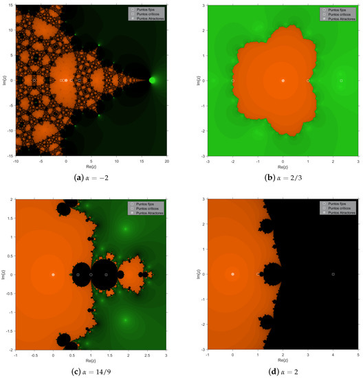
Figure 5.
Dynamical planes for different values of

Figure 6.
Dynamical plane for and a maximum of 100 iterations.
In Figure 7 we can observe the dynamical planes corresponding to Chebyshev (), Halley (), SuperHalley () and Osada’s method () for multiple roots taking . Although each of these methods has three strange fixed points, they are not attracting. As for the first three methods , they can converge to the single root. Moreover, Osada’s method has a wide black area of convergence to the attracting periodic orbit .

Figure 7.
Dynamical planes for (a) Chebyshev; (b) Halley; (c) SuperHalley; (d) Osada.
Finally, we show in Figure 8 the dynamical planes associated with values of the parameter with attracting strange fixed points. For , the strange fixed point is superattracting, while if , and are attracting, so we can observe their basins of attraction represented in red and blue. Both values of correspond to points represented in black in the parameters plane, so they are unstable methods.

Figure 8.
Dynamical planes for different values of .
4. Numerical Test
In order to analyze the behavior of the family for solving multiple-root nonlinear equations, this section performs a numerical test on different problems.
The computations have been performed using MATLAB R2017b. We use of variable precision arithmetic with 50 digits of mantissa. We consider that the solution has been obtained when the absolute difference of two iterates is lower than . If the iterative method needs more than 50 iterations to reach the solution, we consider that the procedure does not converge (N.C.).
We compare the features of our family for with other members included in the family like Chebyshev’s () and SuperHalley’s () methods.
Table 2, Table 3 and Table 4 collect the results of the numerical test on different nonlinear functions with multiple roots. They display the method, the initial guess (), the amount of iterates to reach the multiple root (# iter), the difference between the two last iterates () and the approximated computational order of convergence (ACOC) [30].
Table 2.
Numerical results for the test function .
Table 3.
Numerical results for the test function .
Table 4.
Numerical results for the test function .
The first nonlinear function under study is
Let us note that this function has a double real root for and a single root for . Table 2 shows the results of the iterative methods for two different initial estimations for reaching the double real root.
The second nonlinear function under study is
that has two double real roots: and . Table 3 collects the values resulting from the application of the iterative methods to solve .
The third nonlinear function is
that has a root with multiplicity 9. Table 4 displays the resulting results.
5. Conclusions
A new family of iterative methods for solving multiple-root nonlinear equations based on weight functions with parameters has been introduced.
The introduced family satisfies the scaling theorem. Therefore, the stability analysis is simplified. A complete dynamical analysis of the family – including the analysis of the fixed and critical points, or the parameters and stability planes – has been performed. This study allows the selection of the best members of the family in terms of stability, with the help of the stability and the parameters planes. For a wide set of values of , we can guarantee the convergence to the desired root, as the dynamical planes show.
Selected members of the family have been tested in a numerical comparison with other well-known methods. The use of nonlinear functions with multiple roots evidences in the numerical results that the proposed family is competitive with the rest of the methods.
Author Contributions
Conceptualization, F.I.C.; methodology, N.G.; software, R.A.C.; validation, R.C.; formal analysis, R.A.C.; investigation, R.A.C.; resources, N.G.; data curation, N.G.; writing—original draft preparation, R.A.C.; writing—review and editing, F.I.C.; visualization, R.A.C.; supervision, F.I.C.; project administration, F.I.C.; funding acquisition, F.I.C. All authors have read and agreed to the published version of the manuscript.
Funding
This research was partially supported by Ministerio de Ciencia, Innovación y Universidades under grant PGC2018-095896-B-C22 (MCIU/AEI/FEDER/UE).
Acknowledgments
The authors would like to thank the anonymous reviewers for their comments and suggestions that have improved this manuscript.
Conflicts of Interest
The authors declare no conflict of interest.
References
- Amat, S.; Busquier, S.; Plaza, S. Chaotic dynamics of a third-order Newton-type method. J. Math. Anal. Appl. 2010, 366, 24–32. [Google Scholar] [CrossRef]
- Chicharro, F.I.; Cordero, A.; Gutiérrez, J.M.; Torregrosa, J.R. Complex dynamics of derivative-free methods for nonlinear equations. Appl. Math. Comput. 2013, 219, 7023–7035. [Google Scholar] [CrossRef]
- Chicharro, F.I.; Cordero, A.; Garrido, N.; Torregrosa, J.R. Generating root-finder iterative methods of second order: Convergence and stability. Axioms 2019, 8, 55. [Google Scholar] [CrossRef]
- Chun, C.; Lee, M.Y.; Neta, B.; Dzunic, J. On optimal fourth-order iterative methods free from second derivative and their dynamics. Appl. Math. Comput. 2012, 218, 6427–6438. [Google Scholar] [CrossRef]
- Iliev, A.; Kyurkchiev, N. Nontrivial Methods in Numerical Analysis (Selected Topics in Numerical Analysis); Lambert Academy: Plovdiv, Bulgary, 2010. [Google Scholar]
- Salimi, M.; Behl, R. Sixteenth-order optimal iterative scheme based on inverse interpolatory rational function for nonlinear equations. Symmetry 2019, 11, 691. [Google Scholar] [CrossRef]
- Babajee, D.K.R.; Thukral, R. On a 4-point sixteenth-order King family of iterative methods for solving nonlinear equations. Int. J. Math. Math. Sci. 2012, 2012, 979245. [Google Scholar] [CrossRef]
- Sharma, J.R.; Guha, R.K.; Gupta, P. Improved King’s methods with optimal order of convergence based on rational approximations. Appl. Math. Lett. 2013, 26, 473–480. [Google Scholar] [CrossRef]
- Ignatova, N.; Kyurkchiev, N.; Iliev, A. Multipoint algorithms arising from optimal in the sense of Kung-Traub iterative procedures for numerical solution of nonlinear equations. Gen. Math. Notes 2011, 6, 45–79. [Google Scholar]
- Cordero, A.; Torregrosa, J.R. Chapter On the design of optimal iterative methods for solving nonlinear equations. In Advances in Iterative Methods for Nonlinear Equations; Springer: Cham, Switzerland, 2016; pp. 79–111. [Google Scholar]
- Petkovic, M.S.; Petkovic, L.D. Construction and efficiency of multipoint root-ratio methods for finding multiple zeros. J. Comput. Appl. Math. 2019, 351, 54–65. [Google Scholar] [CrossRef]
- Petkovic, I.; Neta, B. On an application of symbolic computation and computer graphics to root-finders: The case of multiple roots of unknown multiplicity. J. Comput. Appl. Math. 2016, 308, 215–230. [Google Scholar] [CrossRef]
- Proinov, P.D.; Vasileva, M. Local and semilocal convergence of Nourein?s iterative method for finding all zeros of a polynomial simultaneously. Symmetry 2020, 12, 1801. [Google Scholar] [CrossRef]
- Rall, L. Convergence of Newton’s process to multiple solutions. Numer. Math. 1966, 9, 23–37. [Google Scholar] [CrossRef]
- Schröder, E. On infinitely many algorithms. Tech. Rep. 1992, 57, 92–121. [Google Scholar]
- Mora, M. Estabilidad de los métodos Iterativos Para la Aproximación de raíces múltiples de Ecuaciones no Lineales. Master’s Thesis, Universitat Politècnica de València, València, Spain, 2019. [Google Scholar]
- Behl, R.; Cordero, A.; Motsa, S.S.; Torregrosa, J.R. On developing fourth-order optimal families of methods for multiple roots and their dynamics. Appl. Math. Comput. 2015, 265, 520–532. [Google Scholar] [CrossRef]
- Geum, Y.H.; Kim, Y.I.; Neta, B. A family of optimal quartic-order multiple-zero finders with a weight function of the principal kth root of a derivative-to-derivative ratio and their basins of attraction. Math. Comput. Simul. 2017, 136, 1–21. [Google Scholar] [CrossRef]
- Geum, Y.H.; Kim, Y.I.; Neta, B. Constructing a family of optimal eighth-order modified Newton-type multiple-zero finders along with the dynamics behind their purely imaginary extraneous fixed points. J. Comput. Appl. Math. 2018, 333, 121–156. [Google Scholar] [CrossRef]
- Cordero, A.; Jaiswal, J.P.; Torregrosa, J.R. Stability analysis of fourth-order iterative method for finding multiple roots of nonlinear equations. Appl. Math. Nonl. Sci. 2019, 4, 43–56. [Google Scholar]
- Akram, S.; Zafar, F.; Yasmin, N. An optimal eighth-order family of iterative methods for multiple roots. Mathematics 2019, 7, 672. [Google Scholar] [CrossRef]
- Blanchard, P. Complex analytic dynamics on the Riemann sphere. Bull. AMS 1984, 11, 85–141. [Google Scholar] [CrossRef]
- Devaney, R.L. An Introduction to Chaotic Dynamical Systems; Addison-Wesley: Redwood, CA, USA, 1989. [Google Scholar]
- Schlag, W. A Course in Complex Analysis and Riemann Surfaces; American Mathematical Society: Providence, RI, USA, 2014. [Google Scholar]
- Gutiérrez, J.M.; Plaza, S.; Romero, N. Dynamics of a fifth-order iterative method. Int. J. Comput. Math. 2012, 89, 822–835. [Google Scholar] [CrossRef]
- Cordero, A.; Giménez-Palacios, I.; Torregrosa, J.R. Avoiding strange attractors in efficient parametric families of iterative methods for solving nonlinear problems. Appl. Numer. Math. 2019, 137, 1–18. [Google Scholar] [CrossRef]
- Amiri, A.; Cordero, A.; Darvishi, M.T.; Torregrosa, J.R. Stability analysis of a parametric family of seventh-order iterative methods for solving nonlinear systems. Appl. Math. Comput. 2018, 323, 43–57. [Google Scholar] [CrossRef]
- Chicharro, F.I.; Cordero, A.; Garrido, N.; Torregrosa, J.R. On the choice of the best members of the Kim family and the improvement of its convergence. Math. Meth. Appl. Sci. 2019, 43, 8051–8066. [Google Scholar] [CrossRef]
- Chicharro, F.I.; Cordero, A.; Torregrosa, J.R. Drawing dynamical and parameters planes of iterative families and methods. Sci. World J. 2013, 2013, 1–8. [Google Scholar] [CrossRef]
- Cordero, A.; Torregrosa, J.R. Variants of Newton’s method using fifth-order quadrature formulas. Appl. Math. Comput. 2007, 190, 686–698. [Google Scholar] [CrossRef]


Publisher’s Note: MDPI stays neutral with regard to jurisdictional claims in published maps and institutional affiliations. |
© 2020 by the authors. Licensee MDPI, Basel, Switzerland. This article is an open access article distributed under the terms and conditions of the Creative Commons Attribution (CC BY) license (http://creativecommons.org/licenses/by/4.0/).