The Exponentiated Burr–Hatke Distribution and Its Discrete Version: Reliability Properties with CSALT Model, Inference and Applications

Abstract

Continuous and discrete distributions are essential to model both continuous and discrete lifetime data in several applied sciences. This article introduces two extended versions of the Burr–Hatke model to improve its applicability. The first continuous version is called the exponentiated Burr–Hatke (EBuH) distribution. We also propose a new discrete analog, namely the discrete exponentiated Burr–Hatke (DEBuH) distribution. The probability density and the hazard rate functions exhibit decreasing or upside-down shapes, whereas the reversed hazard rate function. Some statistical and reliability properties of the EBuH distribution are calculated. The EBuH parameters are estimated using some classical estimation techniques. The simulation results are conducted to explore the behavior of the proposed estimators for small and large samples. The applicability of the EBuH and DEBuH models is studied using two real-life data sets. Moreover, the maximum likelihood approach is adopted to estimate the parameters of the EBuH distribution under constant-stress accelerated life-tests (CSALTs). Furthermore, a real data set is analyzed to validate our results under the CSALT model.

1. Introduction

Statistical distributions are very important in predicting and describing different real-world phenomena. Choosing a probability distribution that should be utilized to make inference about the real-life data under study is a critical issue in statistics. Hence, considerable efforts over the last few years have been expended in constructing more flexible generalized distributions to model several real data sets encountered in different applied fields such as medicine, insurance, economics, engineering, and agriculture, among others.

Exponentiated models and their successful applications in several applied sciences have been prevalent in the statistical literature. Moreover, one of the most widely adopted generalization techniques is the exponentiated-G (Exp-G) class that can be traced back to [1]. This technique of generalization has received significant attention in the last three decades, and more than forty Exp-G distributions have been published. Some notable models include the Exp-Weibull [2], Exp-exponential [3], Exp-gamma, Exp-Fréchet and Exp-Gumbel [4], Exp-generalized modified-Weibull [5], Exp-Weibull Pareto [6], Exp-Weibull family [7], and Exp Chen-G family [8], among others.

On the other hand, discrete distributions have their importance in modeling count data encountered in many applied fields such as biology, insurance, medicine, life testing, and engineering. Recently, several statisticians constructed new, more flexible discrete models using different discretization techniques and discrete analogs. For example, discrete Burr–Hatke [9], natural discrete Lindley [10], uniform Poisson–Ailamujia [11], and transmuted record type geometric distributions [12].

The aim of the current paper is five-fold as follows:

• Introducing a more flexible two-parameter version of the Burr–Hatke (BuH) distribution [13] based on the exponentiated-G (E-G) family. The proposed model is called the exponentiated Burr–Hatke (EBuH) distribution. Some statistical and reliability properties of the EBuH distribution are derived in explicit forms. This distribution includes the BuH model as a special case, and it can provide decreasing and unimodal hazard shapes.
• Proposing a discrete version of the new EBuH distribution called the discrete exponentiated Burr–Hatke (DEBuH) distribution based on the survival discretization approach. The DEBuH distribution with a decreasing hazard rate shape fits real-life data better than eight competing discrete models.
• Discussing the estimation of the EBuH parameters using eight classical approaches of estimation, including the maximum likelihood estimators (MLE), Cramér–von Mises estimators (CVME), maximum product of spacing estimators (MPSE), right-tail Anderson–Darling estimators (RADE), least-squares estimators (LSE), Anderson–Darling estimators (ADE), percentile-based estimators (PCE), and weighted least-squares estimators (WLSE). The simulation results are conducted to assess the performance of the estimators and compare between them to determine the best approach to estimate the EBuH parameters.
• Studying the empirical importance of the EBuH and DEBuH distributions using two real-life data sets, illustrating that the two introduced models compare very well with other competing continuous and discrete distributions in modeling data.
• Discussing the estimation of the EBuH parameters using the maximum likelihood under CSALT. Further, the EBuH distribution is fitted to a CSALT data set.

The paper is outlined in eight sections. In Section 2, we define the new EBuH distribution. We derive its properties in Section 3. We define the discrete version of the EBuH distribution in Section 4. The EBuH parameters are estimated using several approaches of estimation in Section 5. The simulation results are also investigated in the same section. Section 6 illustrates the potentiality and importance of the new two distributions by using two real-life data sets. We consider the estimation of the two parameters of the EBuH under CSALT model and validate the results using a real data set in Section 7. Section 8 presents some conclusions.

2. The EBuH Distribution

Maniu and Voda [13] proposed the continuous BuH model, which is specified by the following CDF

$$G(x;\alpha )=1-\frac{e^{-\alpha x}}{x+1},x>0,$$

(1)

where $\alpha >0$ is a shape parameter. In this section, we introduce a new generalization of the BuH model based on the exponentiated technique (adding another shape parameter to the base CDF) to increase the flexibility of this distribution in modeling various types of data in different fields. The newly generated model is called the EBuH distribution. The CDF and PDF of the EBuH distribution can be formulated, respectively, as

$$F(x;\alpha ,\beta )={\left(1-\frac{e^{-\alpha x}}{x+1}\right)}^{\beta },x>0$$

(2)

and

$$f(x;\alpha ,\beta )=\frac{\beta (\alpha x+\alpha +1){\left(1+x-e^{-\alpha x}\right)}^{\beta -1}}{{\left(x+1\right)}^{\beta +1}}{e}^{-\alpha x},x>0,$$

(3)

where $\alpha >0$ and $\beta >0$ are shape parameters. The asymptotic behavior of the PDF is

$$f(x;\alpha ,\beta )\sim \left\{\begin{array}{cc}\beta (\alpha +1)x^{\beta -1},& x\to 0,\\ \frac{\alpha \beta }{1+x}exp(-\alpha x),& x\to \infty .\end{array}\right.$$

(4)

A physical interpretation of the EBuH model based on the newly added parameter $\beta$ can be provided as follows. Let $\beta >0$ be an integer number and let $X_1,...,X_{\beta }$ be a random sample from the BuH distribution with shape parameter $\alpha$. If we define $X=max(X_1,...,X_{\beta })$, then the distribution of X leads to the EBuH distribution, which certainly can be used to model the last failure time of a random sample from the BuH distribution.

The following proposition summarizes the possible shape properties for the PDF of the EBuH distribution.

Proposition 1.

The PDF of the EBuH distribution is decreasing for $0<\beta \le 1.$ It is unimodal for $\beta >1,$ where the mode is the root of the following nonlinear equation

$$(\beta -1)\left(1+\alpha (1+x)\right)\left[1+\alpha exp(-\alpha x)\right]={\alpha }^2{(1+x)}^2\left[1+x-exp(-\alpha x)\right]+v\left(x\right),$$

where

$$v\left(x\right)=\frac{(\beta +1)}{1+x}(1+\alpha (x+1))\left[1+x-exp(-\alpha x)\right].$$

Proof. 

Let

$$\begin{array}{cc}\hfill g\left(x\right)& =ln\left[f\right(x,\alpha ,\beta \left)\right]=ln[1+\alpha (x+1\left)\right]+(\beta -1)ln[1+x-exp(-\alpha x\left)\right]\hfill \\ \hfill & -\alpha x-(\beta +1)ln[1+x].\hfill \end{array}$$

By differentiating the above equation with respect to x, followed by rearranging the terms, it follows that

$$g^{{}^{\prime }}\left(x\right)=-{\alpha }^2\frac{1+x}{1+(1+x)\alpha }+(\beta -1)\frac{1+\alpha exp(-\alpha x)}{1+x-exp(-\alpha x)}-\frac{\beta +1}{1+x}.$$

(5)

Clearly, when $\beta \le 1,$ we have $g^{{}^{\prime }}\left(x\right)<0$ for $\forall x>0.$ Therefore, $g\left(x\right)$ is a decreasing function, and hence the PDF of the EBuH distribution is a decreasing function. Next, suppose that $\beta >1,$ and Equation (5) is rewritten as follows:

$$g^{{}^{\prime }}\left(x\right)=\frac{\Delta \left(x\right)}{(\frac{1}{1+x}+\alpha )\left(1-\frac{exp(-\alpha x)}{1+x}\right)},$$

where

$$\begin{array}{cc}\hfill \Delta \left(x\right)& =-\left[{\alpha }^2+\frac{\beta +1}{(1+x)}\left(\frac{1}{1+x}+\alpha \right)\right]\left(1-\frac{exp(-\alpha x)}{1+x}\right)\hfill \\ \hfill & +(\beta -1)\left(\frac{1}{1+x}+\alpha \right)\left[\frac{1+\alpha exp(-\alpha x)}{1+x}\right].\hfill \end{array}$$

Clearly, $g^{{}^{\prime }}\left(x\right)=0$ if and only if $\Delta \left(x\right)=0$. Assume that there exists a root, say $x_0>0$, for Equation (5). It then follows that $g^{{}^{\prime }}\left(x_0\right)=\Delta \left(x_0\right)=0.$ Observe now that ${lim}_{x\to 0}\Delta \left(x\right)={(1+\alpha )}^2(\beta -1)>0$ and ${lim}_{x\to \infty }\Delta \left(x\right)=-{\alpha }^2.$ Immediately, it follows that ${lim}_{x\to 0}{g}^{{}^{\prime }}\left(x\right)=(1+\alpha )(\beta -1){lim}_{x\to 0}{\left(1-\frac{exp(-\alpha x)}{1+x}\right)}^{-1}=+\infty$ and ${lim}_{x\to \infty }{g}^{{}^{\prime }}\left(x\right)=-\alpha .$ This implies that $f(x;\alpha ,\beta )$ is an increasing function for $x<x_0$ and a decreasing function for $x>x_0.$ So, the PDF of the EBuH distribution is a unimodal function with a mode that occurs at $x_0.$ □

Figure 1 shows that the PDF of the EBuH model can be decreasing or unimodal as proved in Proposition 1.

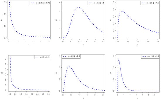
Figure 1. Some possible shapes for the PDF of the EBuH distribution.

3. Properties of the EBuH Distribution

3.1. Moment and Related Measures

If $X\sim$ EBuH$\left(\alpha ,\beta \right)$, the rth moment of X can be formulated as

$${\mu }_r^{\prime }=\underset{0}{\overset{\infty }{\int }}{x}^{r}f(x;\alpha ,\beta )dx.$$

(6)

Using the negative binomial series, Equation (3) can be expressed in a simple form as follows:

$$\begin{array}{ccc}\hfill f(x;\alpha ,\beta )& =& \beta (\alpha x+\alpha +1)\sum _{j=0}^{\infty }\frac{{(-1)}^j\Gamma \left(\beta \right)}{j!{(x+1)}^{j+2}\Gamma (\beta -j)}{e}^{-\alpha (j+1)x}\hfill \\ & =& \beta (\alpha x+\alpha +1)\sum _{j,k=0}^{\infty }\frac{{(-1)}^{j+k}\Gamma \left(\beta \right)}{j!\Gamma (\beta -j)}\left(\genfrac{}{}{0pt}{}{j+k+1}{k}\right)x^k{e}^{-\alpha (j+1)x}\hfill \\ & =& \beta \sum _{j,k=0}^{\infty }{\Theta }_{\beta }^{(j,k)}\left[\alpha x^{k+1}+(\alpha +1)x^k\right]e^{-\alpha (j+1)x},\hfill \end{array}$$

(7)

where

$${\Theta }_{\beta }^{(j,k)}=\frac{{(-1)}^{j+k}\Gamma \left(\beta \right)}{j!\Gamma (\beta -j)}\left(\genfrac{}{}{0pt}{}{j+k+1}{k}\right).$$

Using Equations (6) and (7), we get

$$\begin{array}{ccc}\hfill {\mu }_r^{\prime }& =& \beta \sum _{j,k=0}^{\infty }{\Theta }_{\beta }^{(j,k)}\left[\alpha \underset{0}{\overset{\infty }{\int }}{x}^{r+k+1}{e}^{-\alpha (j+1)x}dx+(\alpha +1)\underset{0}{\overset{\infty }{\int }}{x}^{r+k}{e}^{-\alpha (j+1)x}dx\right]\hfill \\ & =& \beta \sum _{j,k=0}^{\infty }{\Theta }_{\beta }^{(j,k)}\frac{\left(r+k+1\right)(j+1)(\alpha +1)}{{\left(j+1\right)}^{r+k+2}{\alpha }^{r+k+1}}\Gamma \left(r+k+1\right),\hfill \end{array}$$

(8)

where $\left(r+k+1\right)\ne 0,-1,-2,-3,...$.

The qth incomplete moment of X can be expressed as follows

$$\begin{array}{ccc}\hfill {\mathsf{\Phi }}_{\left(q\right)}\left(x\right)& =& {\int }_0^x{t}^{q}f(t;\alpha ,\beta )dx\hfill \\ & =& \beta \sum _{j,k=0}^{\infty }{\Theta }_{\beta }^{(j,k)}\left[\alpha \underset{0}{\overset{x}{\int }}{t}^{q+k+1}{e}^{-\alpha (j+1)t}dt+(\alpha +1)\underset{0}{\overset{x}{\int }}{t}^{q+k}{e}^{-\alpha (j+1)t}dt\right]\hfill \\ & =& \beta \sum _{j,k,m=0}^{\infty }{\Theta }_{\beta }^{(j,k)}\frac{{[-\alpha (j+1)]}^m}{m!}\left[\frac{\alpha x^{q+k+m+2}}{q+k+m+2}+\frac{(\alpha +1)x^{q+k+m+1}}{q+k+m+1}\right].\hfill \end{array}$$

(9)

Table 1 lists some statistical computations of the EBuH model for various values of the model parameters.

Table 1. Some descriptive statistics of the EBuH model.

Parameter		Measure
$\mathit{\alpha }$	$\mathit{\beta }$	Mean	Variance	Skewness	Kurtosis	Index of Dispersion
$0.05$	$0.05$	$0.169113$	$1.784937$	$23.90187$	$970.79179$	$10.554675$
	$0.50$	$1.459027$	$15.63631$	$8.167996$	$115.04027$	$10.716944$
	$1.50$	$3.551243$	$38.64713$	$5.233569$	$48.62806$	$10.88270$
	$2.00$	$4.390324$	$47.91511$	$4.702076$	$39.76626$	$10.91379$
$0.50$	$0.05$	$0.068414$	$0.116458$	$10.88104$	$186.8619$	$1.702242$
	$0.50$	$0.549573$	$0.838333$	$3.813721$	$26.06214$	$1.525425$
	$1.50$	$1.208888$	$1.613429$	$2.579902$	$13.83731$	$1.334638$
	$2.00$	$1.442168$	$1.843117$	$2.370207$	$12.22692$	$1.278018$
$1.50$	$0.05$	$0.034694$	$0.024182$	$8.886853$	$120.2940$	$0.697004$
	$0.50$	$0.272041$	$0.160844$	$3.067550$	$17.40487$	$0.591247$
	$1.50$	$0.578837$	$0.280556$	$2.078336$	$9.931718$	$0.484689$
	$2.00$	$0.682764$	$0.310802$	$1.919330$	$9.004244$	$0.455212$
$2.00$	$0.05$	$0.028164$	$0.015420$	$8.596504$	$111.7193$	$0.547495$
	$0.50$	$0.219971$	$0.101137$	$2.952361$	$16.22215$	$0.459776$
	$1.50$	$0.465489$	$0.173284$	$1.995780$	$9.358395$	$0.372262$
	$2.00$	$0.548039$	$0.190881$	$1.843722$	$8.520078$	$0.348298$

From Table 1, it is clear that the EBuH distribution can be used to model positively skewed and leptokurtic data sets. Moreover, the proposed model is suitable for studying data suffering from over- and under-dispersed data where the index of dispersion “variance to mean ratio” >(<) 1.

3.2. Hazard Rate Function and Availability

If $X\sim$ EBuH$\left(\alpha ,\beta \right)$, then the hazard rate function (HRF) can be expressed by utilizing the well-known relationship $h(x;\alpha ,\beta )=\frac{f(x;\alpha ,\beta )}{R(x;\alpha ,\beta )}$, where $R(x;\alpha ,\beta )=1-F(x;\alpha ,\beta )$ represents the reliability function (RF) of the EBuH distribution. The asymptotic behavior of the HRF is given by

$$\begin{array}{c}\hfill h(x;\alpha ,\beta )\sim \left\{\begin{array}{cc}\beta (\alpha +1)x^{\beta -1},& x\to 0,\\ \alpha ,& x\to \infty .\end{array}\right.\end{array}$$

(10)

Note that for $\beta <1,$ it is observed that the HRF is a decreasing function. The following proposition provides possible shape properties for the HRF of the EBuH distribution.

Proposition 2.

The HRF of the EBuH distribution is decreasing for $0<\beta \le 1$ and is upside-down shaped (unimodal) for $\beta >1.$ In the last scenario, the turning point (mode) of the HRF can be determined as the root for the following equation:

$$(\beta -1)\frac{\left[{\alpha }^2(1+x)+2\alpha +exp\left(\alpha x\right)\right]exp(-\alpha x)}{{(1+x-exp(-\alpha x))}^2}=\frac{\beta {\alpha }^2{(1+x)}^2-(\beta +1)[1+2\alpha (1+x)]}{{(1+x)}^2{(1+\alpha (1+x))}^2}.$$

Proof. 

Put $\psi \left(x\right)=-(\partial /\partial x)[ln(f(x,\alpha ,\beta )\left)\right].$ Then

$$\psi \left(x\right)=\frac{{\alpha }^2(1+x)}{(1+\alpha (1+x\left)\right)}-(\beta -1)\frac{1+\alpha exp(-\alpha x)}{1+x-exp(-\alpha x)}+\frac{\beta +1}{1+x}.$$

The first derivative of $\psi \left(x\right)$ is

$$\begin{array}{cc}\hfill {\psi }^{{}^{\prime }}\left(x\right)& =(\beta -1)\frac{\left[{\alpha }^2(1+x)+2\alpha +exp\left(\alpha x\right)\right]exp(-\alpha x)}{{(1+x-exp(-\alpha x))}^2}\hfill \\ \hfill & -\frac{\beta {\alpha }^2{(1+x)}^2+(\beta +1)[1+2\alpha (1+x)]}{{(1+x)}^2{(1+\alpha (1+x))}^2}.\hfill \end{array}$$

(11)

It can be easily seen that ${\psi }^{{}^{\prime }}\left(x\right)<0$ whenever $0<\beta \le 1,$ and hence it follows from Glaser’s theorem [14] that the HRF is a decreasing function. Next, suppose that $\beta >1$ and suppose there exists $x_0$ such that ${\psi }^{{}^{\prime }}\left(x_0\right)=0.$

Observe that

$$\underset{x\to 0^{+}}{lim}{\psi }^{{}^{\prime }}\left(x\right)=(\beta -1){(1+\alpha )}^2\underset{x\to 0^{+}}{lim}\frac{1}{{(1+x-exp(-\alpha x))}^2}-\frac{\xi (\alpha ,\beta )}{{(1+\alpha )}^2},$$

where $\xi (\alpha ,\beta )=\beta {\alpha }^2+(\beta +1)(1+2\alpha ).$ Due to the assumption that $\beta >1,$ it follows that ${lim}_{x\to 0^{+}}{\psi }^{{}^{\prime }}\left(x\right)=+\infty .$ Note that the first term in Equation (11) is positive for all $x>0$ since $\beta >1$, whereas the second term is negative for all $x>0.$ Consequently, we have (for $\beta >1$)

$$\underset{x\to \infty }{lim}{\psi }^{{}^{\prime }}\left(x\right)\le (\beta -1){(1+\alpha )}^2\underset{x\to \infty }{lim}\frac{1}{{(1+x-exp(-\alpha x))}^2}=0.$$

Therefore, $\psi \left(x\right)$ has a root at $x=x_0$ with ${\psi }^{{}^{\prime }}\left(x\right)>0$ for all $x<x_0$ and ${\psi }^{{}^{\prime }}\left(x\right)<0$ for all $x>x_0.$ Since ${lim}_{x\to 0^{+}}f(x,\alpha ,\beta )=0,$ it then follows from Glaser’s theorem that the HRF of the EBuH distribution is upside-down shaped. □

Figure 2 shows the plots of the HRF for some values of the parameters $\alpha$ and $\beta$. It is evident that the HRF can be decreasing or upside-down shaped. Further, it can be seen that the HRF converges to $\alpha$ for large values of x (see Equation (10)).

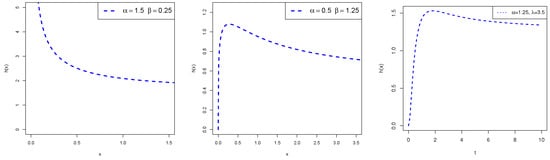
Figure 2. Some possible shapes for the HRF of the EBuH distribution.

3.3. Reversed Hazard Rate Function

The reversed HRF (RHRF) for an absolutely continuous random variable x is defined as the ratio between the PDF of X and its corresponding CDF as follows:

$$\begin{array}{c}\hfill r^{\ast }(x;\alpha ,\beta )=\frac{\partial ln\left(F\right(x,\alpha ,\beta \left)\right)}{\partial x}=\frac{f(x;\alpha ,\beta )}{F(x;\alpha ,\beta )}.\end{array}$$

(12)

It can be considered as one of reliability functions that can be used to identify lifetime variables. In addition, it can be interpreted as the instantaneous rate of increase in the RF. The RHRF of the two-parameter EBuH distribution has the form

$$\begin{array}{c}\hfill r^{\ast }(x;\alpha ,\beta )=\frac{\beta exp(-\alpha x)}{{\left(1+x-exp(-\alpha x)\right)}^2}.\end{array}$$

(13)

The following proposition illustrates that the RHRF of the EBuH distribution is deceasing for all $\alpha ,\beta >0$.

Proposition 3.

The RHRF of the EBuH distribution is deceasing for all $\alpha ,\beta >0$.

Proof. 

On differentiating Equation (13), we obtain the following:

$$\frac{\partial r^{\ast }(x;\alpha ,\beta )}{\partial x}=-\frac{\beta \left[\alpha (1+x-exp(-\alpha x\left)\right)+2\right]exp(-\alpha x)}{{\left(1+x-exp(-\alpha x)\right)}^3}<0,$$

and hence the result follows. □

3.4. The Odds Function

The odds function (OF) at time x is defined as the quotient between the RF and the CDF as follows:

$$OF\left(x\right)=\frac{F\left(x\right)}{1-F\left(X\right)}.$$

Recently, Lando et al. [15] discussed the problem of examining aging forms of the lifetime in the so-called k-out-n systems. Such systems are of practical interest in engineering reliability. Notable, among the four classes of probability distribution function they considered, they showed that the class identified by the convexity of the OF, say (${\mathcal{F}}_{CO}$ ), is the widest class. Additionally, $F\in {\mathcal{F}}_{CO}$ if and only if the quotient between the HRF and the RF, i.e., $O^{\ast }\left(x\right)=h\left(x\right)/(1-F\left(x\right))$, is an increasing function. Obviously, if h is an increasing function, then $O^{\ast }\left(x\right)$ is also an increasing function. In this subsection, we study the OF of the EBuH distribution. Unfortunately, the HRF of the EBuH distribution (as shown in Proposition 2) can be either decreasing or upside-down, and hence the CDF of the EBuH does not belong to ${\mathcal{F}}_{CO}$. In the following proposition, we show that $O^{\ast }$ can be either increasing or bathtub-shaped.

Proposition 4.

The $O^{\ast }\left(x\right)$ function of the EBuH distribution is increasing for $\beta >1$, and it is bathtub-shaped for $\beta \le 1.$

Proof. 

We have that $O^{\ast }\left(x\right)=h(x;\alpha ,\beta )/(1-F(x;\alpha ,\beta ))$, where $h(x;\alpha ,\beta )$ and $F(x;\alpha ,\beta )$ are the HRF and CDF of the EBuH distribution. Let

$$\begin{array}{cc}\hfill \Lambda (x;\alpha ,\beta )& =ln\left[O^{\ast }(x,\alpha ,\beta )\right]\hfill \\ \hfill & =ln\left(\beta \right)+(\beta -1)ln[1+X-exp(-\alpha x\left)\right]+ln[1+\alpha (1+x\left)\right]-\alpha \hfill \\ \hfill & -(\beta +1)ln(1+x)-2ln[1-F(x;\alpha ,\beta \left)\right].\hfill \end{array}$$

The first derivative of $\Lambda (x;\alpha ,\beta )$ is

$$\begin{array}{c}\hfill {\Lambda }^{{}^{\prime }}(x;\alpha ,\beta )=(\beta -1)\frac{1+\alpha exp(-\alpha x)}{1+x-exp(-\alpha x)}-\rho (x,\alpha ,\beta )+2h(x,\alpha ,\beta ),\end{array}$$

(14)

where

$$\rho (x,\alpha ,\beta )=\frac{{\alpha }^2{(1+x)}^2+(\beta +1)[1+\alpha (1+x)]}{(1+x)(1+\alpha (1+x\left)\right)}.$$

Since $h(x;\alpha ,\beta )\ge 0$ for all $x,$ it then follows that

$${\Lambda }^{{}^{\prime }}(x;\alpha ,\beta )\ge (\beta -1)\frac{1+\alpha exp(-\alpha x)}{1+x-exp(-\alpha x)}-\rho (x,\alpha ,\beta ).$$

If $\beta >1,$ it then follows that

$$\underset{x\to 0}{lim}{\Lambda }^{{}^{\prime }}(x;\alpha ,\beta )\ge (\beta -1)\underset{x\to 0}{lim}\frac{1+\alpha exp(-\alpha x)}{1+x-exp(-\alpha x)}-\underset{x\to 0}{lim}\rho (x,\alpha ,\beta ).$$

Since ${lim}_{x\to 0}\rho (x,\alpha ,\beta )=[{\alpha }^2+(1+\alpha )(\beta +1)]/(1+\alpha ),$ then we have that ${lim}_{x\to 0}{\Lambda }^{{}^{\prime }}(x;\alpha ,\beta )$ > $0.$ On the other hand, since $-\rho (x,\alpha ,\beta )<0,$ it then follows that

$${\Lambda }^{{}^{\prime }}(x;\alpha ,\beta )<(\beta -1)\frac{1+\alpha exp(-\alpha x)}{1+x-exp(-\alpha x)}+2h(x,\alpha ,\beta ).$$

Notice that $2h(x,\alpha ,\beta )\sim 2\alpha$ as $\to \infty$ (see Equation (10)) and $1+x-exp(-\alpha x)\ge 1-exp(-\alpha x).$ So,

$$\underset{x\to \infty }{lim}{\Lambda }^{{}^{\prime }}(x;\alpha ,\beta )<(\beta -1)\underset{x\to \infty }{lim}\frac{(\beta -1)}{1-exp(-\alpha x)}+2\alpha =(\beta -1)+2\alpha .$$

Therefore, we have for all $\beta >1$ that ${lim}_{x\to \infty }{\Lambda }^{{}^{\prime }}(x;\alpha ,\beta )>0.$ Next suppose that $\beta \le 1,$ and assume that there exists a root, say $x_0$, for Equation (14), i.e., ${\Lambda }^{{}^{\prime }}(x_0;\alpha ,\beta )=0.$ As $x\to 0,$ we have that ${lim}_{x\to 0}h(x,\alpha ,\beta )=0$ and ${lim}_{x\to 0}\rho (x,\alpha ,\beta )=[{\alpha }^2+(1+\alpha )(\beta +1)]/(1+\alpha ).$ Therefore, we have ${lim}_{x\to 0}{\Lambda }^{{}^{\prime }}(x;\alpha ,\beta )=-\infty .$

On the other hand, as $x\to \infty ,$ we have $h(x,\alpha ,\beta )\to 2\alpha$ and $\rho (x,\alpha ,\beta )\to \alpha .$ Hence, we have ${\Lambda }_{x\to \infty }^{{}^{\prime }}(x_0;\alpha ,\beta )=\alpha >0.$ Therefore, for all $x<x_0$ we have ${\Lambda }^{{}^{\prime }}(x;\alpha ,\beta )<0$ and for $x>x_0,$ we have ${\Lambda }^{{}^{\prime }}(x;\alpha ,\beta )>0.$ Hence, $\Lambda (x;\alpha ,\beta )$ is bathtub-shaped. □

Notice that the CDF of the EBuH distribution lies in ${\mathcal{F}}_{CO}$ for $\beta >1.$ Figure 3 shows the behavior of the $O^{\ast }$ of the EBuH distribution for some values of $\alpha$ and $\beta$.

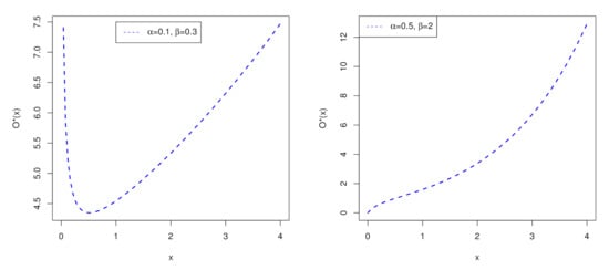
Figure 3. Some possible shapes for the $O^{\ast }$ of the EBuH distribution.

Recall, Equation (8), we can derive some important measures in survival analysis such as the mean time to failure (MTTF), mean time to repair (MTTR), mean time between failures (MTBF), and availability (Av). These measures can be adopted to design and manufacture a maintainable system. Assume $X_1$ represents the time to failure with parameters ${\alpha }_1$ and ${\beta }_1$ ($X_1\sim$ EBuH$\left({\alpha }_1,{\beta }_1\right)$), and $X_2$ represents the time to repair with parameters ${\alpha }_2$ and ${\beta }_2$ ($X_1\sim$ EBuH$\left({\alpha }_1,{\beta }_1\right)$), then MTTF = ${\mu }_1^{\prime }({\alpha }_1,{\beta }_1)$, MTTR = ${\mu }_1^{\prime }({\alpha }_2,{\beta }_2)$, MTBF = ${\mu }_1^{\prime }({\alpha }_1,{\beta }_1)+{\mu }_1^{\prime }({\alpha }_2,{\beta }_2)$, and Av $={\mu }_1^{\prime }({\alpha }_1,{\beta }_1)/\left[{\mu }_1^{\prime }({\alpha }_1,{\beta }_1)+{\mu }_1^{\prime }({\alpha }_2,{\beta }_2)\right]$. The Av is the probability that the system can conduct its required function when it is called upon given that it is not failed or undergoing a repair action. Therefore, the Av is not only a function of reliability, but it is also a function of maintainability. Table 2 reports some reliability computations of the EBuH model for various values of its parameters.

Table 2. Some reliability computations of the EBuH model.

Parameter		Measure
$\mathit{\alpha }$	$\mathit{\beta }$	MTTF	MTTR${}_{\mathit{\alpha }=\mathbf{1}.\mathbf{5}}^{\mathit{\beta }=\mathbf{2}.\mathbf{5}}$	MTBF	Av
$0.05$	$0.05$	$0.169113$	$0.769202$	$0.938315$	$0.180230$
	$0.50$	$1.459027$	$0.769202$	$2.228229$	$0.654792$
	$1.50$	$3.551243$	$0.769202$	$4.320446$	$0.821962$
	$2.00$	$4.390324$	$0.769202$	$5.159527$	$0.850916$
$0.50$	$0.05$	$0.068414$	$0.769202$	$0.837617$	$0.081677$
	$0.50$	$0.549573$	$0.769202$	$1.318775$	$0.416729$
	$1.50$	$1.208888$	$0.769202$	$1.978091$	$0.611139$
	$2.00$	$1.442168$	$0.769202$	$2.211371$	$0.652160$
$1.50$	$0.05$	$0.034694$	$0.769202$	$0.80389$	$0.043157$
	$0.50$	$0.272041$	$0.769202$	$1.041244$	$0.261266$
	$1.50$	$0.578837$	$0.769202$	$1.348039$	$0.429391$
	$2.00$	$0.682764$	$0.769202$	$1.451966$	$0.470234$
$2.00$	$0.05$	$0.028164$	$0.769202$	$0.797367$	$0.035322$
	$0.50$	$0.219971$	$0.769202$	$0.989174$	$0.222379$
	$1.50$	$0.465489$	$0.769202$	$1.234692$	$0.377008$
	$2.00$	$0.548039$	$0.769202$	$1.317242$	$0.416050$

From Table 2, it is observed that the MTTF, MTBF, and Av increase for fixed values of $\alpha$ with the increasing of $\beta$.

4. The DEBuH Distribution

If $X\sim$ EBuH$\left(\alpha ,\beta \right)$, then the CDF of the DEBuH model can be formulated as

$$\Pi (x;p,\beta )={\left(1-\frac{p^{x+1}}{x+2}\right)}^{\beta },x\in {\mathbb{N}}_0,$$

(15)

where $p=e^{-\alpha }$and ${\mathbb{N}}_0=\left\{0,1,2,3,...,s\right\}$ for $0<s<\infty$.

The probability mass function (PMF) of the DEBuH model reduces to

$$\pi (x;p,\beta )={\left(1-\frac{p^{x+1}}{x+2}\right)}^{\beta }-{\left(1-\frac{p^x}{x+1}\right)}^{\beta },x\in {\mathbb{N}}_0.$$

Now, we discuss the shape characteristics of the CDF and PMF of the DEBuH model. The behavior of the CDF and PMF are given, respectively, by

$$\Pi (x;p,\beta )=\left\{\begin{array}{cc}1,& \beta ⟶0,\\ {\left(\frac{x+1}{x+2}\right)}^{\beta },& p⟶1\end{array}\right.$$

(16)

and

$$\pi (x;p,\beta )=\left\{\begin{array}{cc}0,& \beta ⟶0,\\ {\left(\frac{x+1}{x+2}\right)}^{\beta }-{\left(\frac{x}{x+1}\right)}^{\beta },& p⟶1.\end{array}\right.$$

(17)

The HRF can be introduced by using the well-known relationship $h^{\ast }(x;p,\beta )=\frac{\pi (x;p,\beta )}{1-\Pi (x-1;p,\beta )}$. The behavior of the HRF of the DEBuH model is given by

$$h^{\ast }(x;p,\beta )=\left\{\begin{array}{cc}1-\frac{1}{ln\left(1-\frac{p^x}{x+1}\right)}ln\left(1-\frac{p^{x+1}}{x+2}\right);& \beta ⟶0,\\ \frac{{\left(\frac{x}{x+1}\right)}^{\beta }-{\left(\frac{x+1}{x+2}\right)}^{\beta }}{{\left(\frac{x}{x+1}\right)}^{\beta }-1};& p⟶1.\end{array}\right.$$

(18)

Figure 4 and Figure 5 display the PMF and HRF plots for different values of the parameters p and $\beta$.

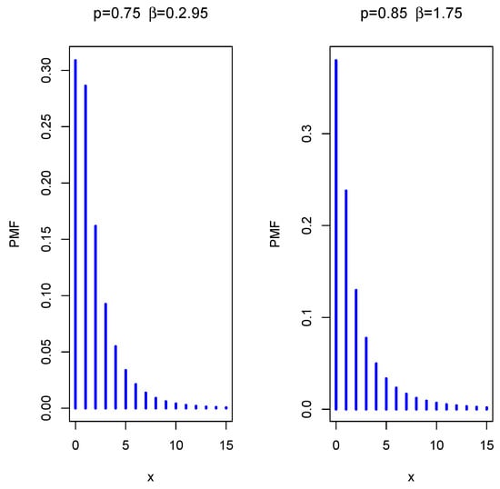
Figure 4. The PMF plots of the DEBuH distribution.

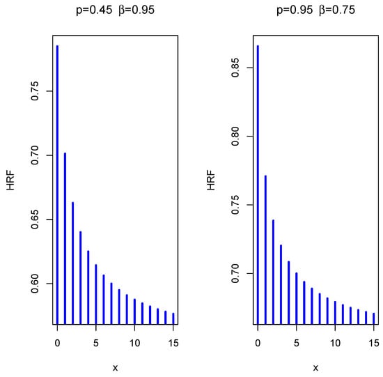
Figure 5. The HRF plots of the DEBuH distribution.

From Figure 4 and Figure 5, it is noted that the PMF and HRF of the DEBuH model are decreasing functions of X.

5. Estimation Methods

In this section, we estimate the unknown parameters $\alpha$ and $\beta$of the EBuH model by utilizing the eight most frequent estimators.

5.1. Maximum Likelihood Estimators

In this section, we present the MLE of the EBuH parameters. Let $x_1,x_2,...,x_m$ be m independent random variables with the EBuH($\alpha ,\beta$) model, then the log-likelihood function, say $L(\alpha ,\beta ;x)$, of the EBuH model can be formulated as

$$\begin{array}{cc}\hfill L(\alpha ,\beta ;x)=& \sum _{j=1}^{m}log\beta (\alpha x_j+\alpha +1)+(\beta -1)\sum _{j=1}^{m}log(1+x_j-e^{-\alpha x_j})\hfill \\ \hfill & -\alpha \sum _{j=1}^m{x}_j-(\beta +1)\sum _{j=1}^{m}log\left(x_j+1\right).\hfill \end{array}$$

To estimate the unknown parameters $\alpha$ and $\beta$, we take the partial derivative of $L(\alpha ,\beta ;x)$ with respect to $\alpha$ and $\beta$, and equate the result equation to zero. The solution can be reported by utilizing the Newton–Raphson procedure.

5.2. Maximum Product of Spacings Estimators

For $j=1,2,\dots ,m+1$, let

$$K_j(\alpha ,\beta )=F\left(x_{\left(j\right)}|\alpha ,\beta \right)-F\left(x_{(j-1)}|\alpha ,\beta \right),$$

be the uniform spacings of a random sample from the EBuH model, where $F\left(x_{\left(0\right)}|\alpha ,\beta \right)=0$, $F\left(x_{(m+1)}|\alpha ,\beta \right)=1$ and ${\sum }_{j=1}^{m+1}{K}_j(\alpha ,\beta )=1$.

The MPSEs of $\alpha$ and $\beta$, say ${\widehat{\alpha }}_{MPS}$ and ${\widehat{\beta }}_{MPS}$, can be derived by maximizing the geometric mean of the spacings

$$G\left(\alpha ,\beta \right)={\left[\prod _{j=1}^{m+1}{K}_j(\alpha ,\beta )\right]}^{\frac{1}{m+1}},$$

with respect to the parameters $\alpha$ and $\beta$.

5.3. Least-Squares Estimators

Let $x_{\left(1\right)},x_{\left(2\right)},\cdots ,x_{\left(m\right)}$ be the order statistics of a random sample from the EBuH model. The LSE of the EBuH parameters, say ${\widehat{\alpha }}_{LS}$ and ${\widehat{\beta }}_{LS}$, can be derived by solving the non-linear equation defined by

$$\sum _{j=1}^m\left[{\left(1-\frac{e^{-\alpha x_j}}{x_j+1}\right)}^{\beta }-\frac{j}{m+1}\right]{\Delta }_l\left(x_{\left(j\right)}|\alpha ,\beta \right)=0;l=1,2,$$

(19)

where

$${\Delta }_1\left(x_{\left(i\right)}|\alpha ,\beta \right)=\frac{\partial }{\partial \alpha }{\left(1-\frac{e^{-\alpha x_j}}{x_j+1}\right)}^{\beta }\mathrm{and}{\Delta }_2\left(x_{\left(i\right)}|\alpha ,\beta \right)=\frac{\partial }{\partial \beta }{\left(1-\frac{e^{-\alpha x_j}}{x_j+1}\right)}^{\beta }.$$

(20)

Note that the solution of ${\Delta }_l\left(x_{\left(j\right)}|\alpha ,\beta \right)$ can be obtained numerically.

5.4. Cramer–Von Mises Estimators

The CVME follows as the difference between the estimate of the CDF and the empirical CDF. The CVME of the EBuH parameters can be estimated by solving the non-linear equation defined as

$$\sum _{j=1}^m\left[{\left(1-\frac{e^{-\alpha x_j}}{x_j+1}\right)}^{\beta }-\frac{2j-1}{2m}\right]{\Delta }_l\left(x_{\left(j\right)}|\alpha ,\beta \right)=0;l=1,2,$$

(21)

where ${\Delta }_l\left(x_{\left(j\right)}|\alpha ,\beta \right)$ is defined in Equation (20).

5.5. Percentile Estimator

Let $u_j=j/\left(m+1\right)$ be an unbiased estimator of $F\left(x_{\left(j\right)}|\alpha ,\beta \right)$. Hence, the PCE of the parameters $\alpha$and $\beta$, denoted by ${\widehat{\alpha }}_{PT}$ and ${\widehat{\beta }}_{PT}$, can be reported by minimizing

$$P(\alpha ,\beta )=\sum _{j=1}^m{\left(x_{\left(j\right)}-Q\left(u_j\right)\right)}^2,$$

with respect to the parameters $\alpha$ and $\beta$, where $Q\left(u_j\right)=F^{-1}\left(x_{\left(j\right)}|\alpha ,\beta \right)$ is the quantile function (QF) of the EBuH model.

5.6. Weighted Least-Squares Estimators

The WLSE of the EBuH parameters, say ${\widehat{\alpha }}_{WLS}$ and ${\widehat{\beta }}_{WLS}$, can be derived by solving the non-linear equation defined by

$$\sum _{j=1}^m\frac{{\left(m+1\right)}^2\left(m+2\right)}{j\left(m-j+1\right)}\left[{\left(1-\frac{e^{-\alpha x_j}}{x_j+1}\right)}^{\beta }-\frac{j}{m+1}\right]{\Delta }_l\left(x_{\left(j\right)}|\alpha ,\beta \right)=0,$$

(22)

where ${\Delta }_l\left(x_{\left(j\right)}|\alpha ,\beta \right)$ is provided in Equation (20).

5.7. Anderson–Darling and Right-Tail Anderson–Darling Estimators

The ADE is another type of minimum distance estimator. The ADEs of the EBuH parameters, say ${\widehat{\alpha }}_{AD}$ and ${\widehat{\beta }}_{AD}$, are derived by minimizing

$$AD(\alpha ,\beta )=-m-\frac{1}{m}\sum _{j=1}^m(2j-1)\left[\beta log\left(1-\frac{e^{-\alpha x_j}}{x_j+1}\right)+log\left(1-{\left(1-\frac{e^{-\alpha x_j}}{x_j+1}\right)}^{\beta }\right)\right],$$

with respect to the parameters $\alpha$ and $\beta$, whereas the RADE of the model parameters can be obtained by minimizing

$$RTAD(\alpha ,\beta )=\frac{m}{2}-2\sum _{j=1}^{m}F\left(x_{(j:m)}|\alpha ,\beta \right)-\frac{1}{m}\sum _{j=1}^m(2j-1)\left[log\left(1-F\left(x_{(m+1-j:m)}|\alpha ,\beta \right)\right)\right],$$

with respect to the parameters $\alpha$ and $\beta .$

5.8. Simulation Results

This section is devoted to exploring the performance of several estimators by the following algorithm.

1.

Random samples of sizes $n=20,50,150$ and 300 are generated using the QF of the EBuH distribution. Its QF has the form

$x_i=-1+\frac{1}{\alpha }W\left(\frac{\alpha e^{\alpha }}{u^{1/\beta }-1}\right),i=1,2,\dots ,n.$

2.

The simulation results are obtained based on 8 combinations of the parameters, i.e., $\alpha =0.50,1.50,3.00$ and $\beta =0.50,1.50,3.00$.

3.

Each sample is repeated $N=5000$ times.

4.

The results of average absolute biases $\left|BIAS\right|=\frac{1}{N}{\sum }_{i=1}^N|\widehat{\mathit{\delta }}-\mathit{\delta }|$, the average mean square errors ($MSE$), $MSE=\frac{1}{N}{\sum }_{i=1}^N{(\widehat{\mathit{\delta }}-\mathit{\delta })}^2$, and average mean relative errors ($MRE$), $MRE=\frac{1}{N}{\sum }_{i=1}^N|\widehat{\mathit{\delta }}-\mathit{\delta }|/\mathit{\delta }$, where $\mathit{\delta }={(\alpha ,\beta )}^{{}^{\prime }}$, are computed, using the R software, for all combinations and presented in Table 3, Table 4, Table 5 and Table 6.

Table 3. Simulation results of the eight estimation methods for $\alpha =0.5$ and $\beta =0.5,1.5$.

n	Est	Par	MLE	MPSE	LSE	CVME	WLSE	PCE	ADE	RADE
		$\alpha =0.5$				$\beta =0.5$
20	$\left|Bias\right|$	$\widehat{\alpha }$	$0.23722$	$0.27668$	$0.34071$	$0.32819$	$0.31814$	$0.32973$	$0.28512$	$0.26870$
		$\widehat{\beta }$	$0.08737$	$0.08549$	$0.09428$	$0.09916$	$0.08978$	$0.15681$	$0.08473$	$0.09921$
	$MSE$	$\widehat{\alpha }$	$0.05627$	$0.07655$	$0.11608$	$0.10771$	$0.10121$	$0.10872$	$0.08129$	$0.07220$
		$\widehat{\beta }$	$0.00763$	$0.00731$	$0.00889$	$0.00983$	$0.00806$	$0.02459$	$0.00718$	$0.00984$
	$MRE$	$\widehat{\alpha }$	$0.47443$	$0.55335$	$0.68141$	$0.65639$	$0.63628$	$0.65947$	$0.57024$	$0.53739$
		$\widehat{\beta }$	$0.17475$	$0.17098$	$0.18857$	$0.19832$	$0.17957$	$0.31363$	$0.16946$	$0.19842$
50	$\left|Bias\right|$	$\widehat{\alpha }$	$0.15666$	$0.17705$	$0.20838$	$0.20459$	$0.17955$	$0.21029$	$0.18225$	$0.16923$
		$\widehat{\beta }$	$0.05446$	$0.05683$	$0.05811$	$0.05934$	$0.05943$	$0.12094$	$0.05313$	$0.06225$
	$MSE$	$\widehat{\alpha }$	$0.02454$	$0.03135$	$0.04342$	$0.04186$	$0.03224$	$0.04422$	$0.03321$	$0.02864$
		$\widehat{\beta }$	$0.00297$	$0.00323$	$0.00338$	$0.00352$	$0.00353$	$0.01463$	$0.00282$	$0.00387$
	$MRE$	$\widehat{\alpha }$	$0.31331$	$0.35409$	$0.41676$	$0.40917$	$0.35910$	$0.42058$	$0.36450$	$0.33846$
		$\widehat{\beta }$	$0.10892$	$0.11366$	$0.11622$	$0.11868$	$0.11886$	$0.24188$	$0.10625$	$0.12450$
150	$\left|Bias\right|$	$\widehat{\alpha }$	$0.08750$	$0.09626$	$0.12423$	$0.1177$	$0.10233$	$0.14031$	$0.10166$	$0.09940$
		$\widehat{\beta }$	$0.03092$	$0.03314$	$0.03579$	$0.03553$	$0.03166$	$0.08872$	$0.03261$	$0.03476$
	$MSE$	$\widehat{\alpha }$	$0.00766$	$0.00927$	$0.01543$	$0.01387$	$0.01047$	$0.01969$	$0.01033$	$0.00988$
		$\widehat{\beta }$	$0.00096$	$0.00110$	$0.00128$	$0.00126$	$0.00100$	$0.00787$	$0.00106$	$0.00121$
	$MRE$	$\widehat{\alpha }$	$0.17500$	$0.19252$	$0.24845$	$0.23552$	$0.20467$	$0.28062$	$0.20331$	$0.19880$
		$\widehat{\beta }$	$0.06184$	$0.06629$	$0.07158$	$0.07105$	$0.06331$	$0.17744$	$0.06522$	$0.06952$
300	$\left|Bias\right|$	$\widehat{\alpha }$	$0.06342$	$0.06800$	$0.08196$	$0.08513$	$0.07609$	$0.09662$	$0.06943$	$0.07255$
		$\widehat{\beta }$	$0.02101$	$0.02288$	$0.02474$	$0.02624$	$0.02302$	$0.06228$	$0.02304$	$0.02466$
	$MSE$	$\widehat{\alpha }$	$0.00402$	$0.00462$	$0.00672$	$0.00725$	$0.00579$	$0.00934$	$0.00482$	$0.00526$
		$\widehat{\beta }$	$0.00044$	$0.00052$	$0.00061$	$0.00069$	$0.00053$	$0.00388$	$0.00053$	$0.00061$
	$MRE$	$\widehat{\alpha }$	$0.12685$	$0.13599$	$0.16393$	$0.17025$	$0.15219$	$0.19324$	$0.13886$	$0.14511$
		$\widehat{\beta }$	$0.04202$	$0.04576$	$0.04948$	$0.05247$	$0.04604$	$0.12457$	$0.04609$	$0.04933$
		$\alpha =0.5$				$\beta =1.5$
20	$\left|Bias\right|$	$\widehat{\alpha }$	$0.16642$	$0.19079$	$0.21021$	$0.21342$	$0.19171$	$0.22395$	$0.16993$	$0.17923$
		$\widehat{\beta }$	$0.29323$	$0.29386$	$0.34907$	$0.36117$	$0.29864$	$0.43715$	$0.29031$	$0.34217$
	$MSE$	$\widehat{\alpha }$	$0.02770$	$0.03640$	$0.04419$	$0.04555$	$0.03675$	$0.05016$	$0.02888$	$0.03212$
		$\widehat{\beta }$	$0.08598$	$0.08635$	$0.12185$	$0.13044$	$0.08918$	$0.19110$	$0.08428$	$0.11708$
	$MRE$	$\widehat{\alpha }$	$0.33284$	$0.38159$	$0.42042$	$0.42685$	$0.38342$	$0.44791$	$0.33986$	$0.35846$
		$\widehat{\beta }$	$0.19549$	$0.19591$	$0.23271$	$0.24078$	$0.19909$	$0.29143$	$0.19354$	$0.22811$
50	$\left|Bias\right|$	$\widehat{\alpha }$	$0.10566$	$0.11679$	$0.12932$	$0.12951$	$0.11824$	$0.14983$	$0.11307$	$0.11572$
		$\widehat{\beta }$	$0.18331$	$0.18701$	$0.20858$	$0.21783$	$0.18733$	$0.33351$	$0.18904$	$0.21078$
	$MSE$	$\widehat{\alpha }$	$0.01116$	$0.01364$	$0.01672$	$0.01677$	$0.01398$	$0.02245$	$0.01279$	$0.01339$
		$\widehat{\beta }$	$0.03360$	$0.03497$	$0.04350$	$0.04745$	$0.03509$	$0.11123$	$0.03574$	$0.04443$
	$MRE$	$\widehat{\alpha }$	$0.21132$	$0.23357$	$0.25864$	$0.25902$	$0.23649$	$0.29967$	$0.22614$	$0.23145$
		$\widehat{\beta }$	$0.12221$	$0.12467$	$0.13905$	$0.14522$	$0.12489$	$0.22234$	$0.12603$	$0.14052$
150	$\left|Bias\right|$	$\widehat{\alpha }$	$0.05879$	$0.06331$	$0.07489$	$0.07387$	$0.06563$	$0.08672$	$0.06150$	$0.06668$
		$\widehat{\beta }$	$0.10070$	$0.10767$	$0.12217$	$0.12126$	$0.11415$	$0.21314$	$0.10941$	$0.12615$
	$MSE$	$\widehat{\alpha }$	$0.00346$	$0.00401$	$0.00561$	$0.00546$	$0.00431$	$0.00752$	$0.00378$	$0.00445$
		$\widehat{\beta }$	$0.01014$	$0.01159$	$0.01493$	$0.01470$	$0.01303$	$0.04543$	$0.01197$	$0.01591$
	$MRE$	$\widehat{\alpha }$	$0.11758$	$0.12662$	$0.14978$	$0.14774$	$0.13125$	$0.17345$	$0.12301$	$0.13336$
		$\widehat{\beta }$	$0.06714$	$0.07178$	$0.08145$	$0.08084$	$0.07610$	$0.14209$	$0.07294$	$0.08410$
300	$\left|Bias\right|$	$\widehat{\alpha }$	$0.04119$	$0.04401$	$0.04948$	$0.04997$	$0.04759$	$0.06348$	$0.04638$	$0.04581$
		$\widehat{\beta }$	$0.07171$	$0.07178$	$0.08188$	$0.08412$	$0.07626$	$0.16093$	$0.07559$	$0.08796$
	$MSE$	$\widehat{\alpha }$	$0.00170$	$0.00194$	$0.00245$	$0.00250$	$0.00226$	$0.00403$	$0.00215$	$0.00210$
		$\widehat{\beta }$	$0.00514$	$0.00529$	$0.00670$	$0.00708$	$0.00582$	$0.02590$	$0.00571$	$0.00774$
	$MRE$	$\widehat{\alpha }$	$0.08237$	$0.08801$	$0.09895$	$0.09994$	$0.09517$	$0.12696$	$0.09277$	$0.09162$
		$\widehat{\beta }$	$0.04780$	$0.04850$	$0.05459$	$0.05608$	$0.05084$	$0.10728$	$0.05039$	$0.05864$

Table 4. Simulation results of the eight estimation methods for $\alpha =0.5,1.5$ and $\beta =0.5,3.0$.

n	Est	Par	MLE	MPSE	LSE	CVME	WLSE	PCE	ADE	RADE
		$\alpha =0.5$				$\beta =3.0$
20	$\left|Bias\right|$	$\widehat{\alpha }$	$0.13710$	$0.15163$	$0.16056$	$0.16007$	$0.14606$	$0.17658$	$0.13811$	$0.14064$
		$\widehat{\beta }$	$0.66604$	$0.66802$	$0.73752$	$0.71864$	$0.69278$	$0.92649$	$0.65335$	$0.77032$
	$MSE$	$\widehat{\alpha }$	$0.01880$	$0.02299$	$0.02578$	$0.02562$	$0.02133$	$0.03118$	$0.01907$	$0.01978$
		$\widehat{\beta }$	$0.44361$	$0.44625$	$0.54393$	$0.51645$	$0.47994$	$0.85838$	$0.42687$	$0.59339$
	$MRE$	$\widehat{\alpha }$	$0.27419$	$0.30325$	$0.32111$	$0.32014$	$0.29211$	$0.35317$	$0.27622$	$0.28128$
		$\widehat{\beta }$	$0.22201$	$0.22267$	$0.24584$	$0.23955$	$0.23093$	$0.30883$	$0.21778$	$0.25677$
50	$\left|Bias\right|$	$\widehat{\alpha }$	$0.08079$	$0.09341$	$0.09837$	$0.10138$	$0.08887$	$0.12180$	$0.08980$	$0.09521$
		$\widehat{\beta }$	$0.39722$	$0.43020$	$0.47341$	$0.46289$	$0.41913$	$0.64776$	$0.42198$	$0.48202$
	$MSE$	$\widehat{\alpha }$	$0.00653$	$0.00873$	$0.00968$	$0.01028$	$0.00790$	$0.01483$	$0.00806$	$0.00907$
		$\widehat{\beta }$	$0.15778$	$0.18507$	$0.22412$	$0.21427$	$0.17567$	$0.41959$	$0.17807$	$0.23234$
	$MRE$	$\widehat{\alpha }$	$0.16157$	$0.18683$	$0.19674$	$0.20277$	$0.17773$	$0.24359$	$0.17960$	$0.19043$
		$\widehat{\beta }$	$0.13241$	$0.14340$	$0.15780$	$0.15430$	$0.13971$	$0.21592$	$0.14066$	$0.16067$
150	$\left|Bias\right|$	$\widehat{\alpha }$	$0.04963$	$0.04975$	$0.05792$	$0.05732$	$0.05231$	$0.07053$	$0.05290$	$0.05541$
		$\widehat{\beta }$	$0.22530$	$0.23303$	$0.26602$	$0.27166$	$0.25062$	$0.42233$	$0.24857$	$0.27333$
	$MSE$	$\widehat{\alpha }$	$0.00246$	$0.00247$	$0.00335$	$0.00329$	$0.00274$	$0.00497$	$0.00280$	$0.00307$
		$\widehat{\beta }$	$0.05076$	$0.05430$	$0.07076$	$0.07380$	$0.06281$	$0.17836$	$0.06179$	$0.07471$
	$MRE$	$\widehat{\alpha }$	$0.09925$	$0.09949$	$0.11584$	$0.11464$	$0.10463$	$0.14105$	$0.10580$	$0.11082$
		$\widehat{\beta }$	$0.07510$	$0.07768$	$0.08867$	$0.09055$	$0.08354$	$0.14078$	$0.08286$	$0.09111$
300	$\left|Bias\right|$	$\widehat{\alpha }$	$0.03357$	$0.03566$	$0.04066$	$0.04120$	$0.03662$	$0.05295$	$0.03472$	$0.03936$
		$\widehat{\beta }$	$0.16199$	$0.16688$	$0.19048$	$0.18551$	$0.16784$	$0.31531$	$0.16637$	$0.20481$
	$MSE$	$\widehat{\alpha }$	$0.00113$	$0.00127$	$0.00165$	$0.00170$	$0.00134$	$0.00280$	$0.00121$	$0.00155$
		$\widehat{\beta }$	$0.02624$	$0.02785$	$0.03628$	$0.03441$	$0.02817$	$0.09942$	$0.02768$	$0.04195$
	$MRE$	$\widehat{\alpha }$	$0.06713$	$0.07131$	$0.08132$	$0.08240$	$0.07324$	$0.10590$	$0.06945$	$0.07871$
		$\widehat{\beta }$	$0.05400$	$0.05563$	$0.06349$	$0.06184$	$0.05595$	$0.10510$	$0.05546$	$0.06827$
		$\alpha =1.5$				$\beta =0.5$
20	$\left|Bias\right|$	$\widehat{\alpha }$	$0.55333$	$0.61664$	$0.69601$	$0.68754$	$0.60181$	$0.72988$	$0.55489$	$0.57848$
		$\widehat{\beta }$	$0.09267$	$0.09250$	$0.10210$	$0.10488$	$0.09108$	$0.17221$	$0.09377$	$0.10395$
	$MSE$	$\widehat{\alpha }$	$0.30617$	$0.38025$	$0.03123$	$0.47271$	$0.36218$	$0.53273$	$0.30791$	$0.33464$
		$\widehat{\beta }$	$0.00859$	$0.00856$	$0.00079$	$0.01100$	$0.00830$	$0.02966$	$0.00879$	$0.01080$
	$MRE$	$\widehat{\alpha }$	$0.36888$	$0.41110$	$0.46401$	$0.45836$	$0.40121$	$0.48659$	$0.36993$	$0.38565$
		$\widehat{\beta }$	$0.18535$	$0.18499$	$0.20419$	$0.20977$	$0.18217$	$0.34442$	$0.18754$	$0.20789$
50	$\left|Bias\right|$	$\widehat{\alpha }$	$0.34677$	$0.37896$	$0.41602$	$0.42225$	$0.39230$	$0.49684$	$0.36109$	$0.36519$
		$\widehat{\beta }$	$0.05600$	$0.05969$	$0.06457$	$0.06216$	$0.06002$	$0.13105$	$0.05730$	$0.06699$
	$MSE$	$\widehat{\alpha }$	$0.12025$	$0.14361$	$0.06692$	$0.17830$	$0.15390$	$0.24685$	$0.13038$	$0.13336$
		$\widehat{\beta }$	$0.00314$	$0.00356$	$0.00142$	$0.00386$	$0.00360$	$0.01718$	$0.00328$	$0.00449$
	$MRE$	$\widehat{\alpha }$	$0.23118$	$0.25264$	$0.27734$	$0.28150$	$0.26154$	$0.33122$	$0.24073$	$0.24346$
		$\widehat{\beta }$	$0.11199$	$0.11938$	$0.12914$	$0.12433$	$0.12004$	$0.26211$	$0.11460$	$0.13398$
150	$\left|Bias\right|$	$\widehat{\alpha }$	$0.19410$	$0.20715$	$0.25869$	$0.24023$	$0.22276$	$0.31247$	$0.21283$	$0.20047$
		$\widehat{\beta }$	$0.03126$	$0.03216$	$0.03772$	$0.03478$	$0.03385$	$0.08456$	$0.03483$	$0.03611$
	$MSE$	$\widehat{\alpha }$	$0.03768$	$0.04291$	$0.17307$	$0.05771$	$0.04962$	$0.09764$	$0.04530$	$0.04019$
		$\widehat{\beta }$	$0.00098$	$0.00103$	$0.00417$	$0.00121$	$0.00115$	$0.00715$	$0.00121$	$0.00130$
	$MRE$	$\widehat{\alpha }$	$0.12940$	$0.13810$	$0.17246$	$0.16016$	$0.14851$	$0.20831$	$0.14189$	$0.13364$
		$\widehat{\beta }$	$0.06252$	$0.06433$	$0.07544$	$0.06955$	$0.06770$	$0.16913$	$0.06965$	$0.07221$
300	$\left|Bias\right|$	$\widehat{\alpha }$	$0.13498$	$0.14512$	$0.17673$	$0.18095$	$0.14821$	$0.22005$	$0.15110$	$0.14417$
		$\widehat{\beta }$	$0.02255$	$0.02404$	$0.02808$	$0.02620$	$0.02308$	$0.06334$	$0.02364$	$0.02637$
	$MSE$	$\widehat{\alpha }$	$0.01822$	$0.02106$	$0.48443$	$0.03274$	$0.02197$	$0.04842$	$0.02283$	$0.02078$
		$\widehat{\beta }$	$0.00051$	$0.00058$	$0.01042$	$0.00069$	$0.00053$	$0.00401$	$0.00056$	$0.00070$
	$MRE$	$\widehat{\alpha }$	$0.08999$	$0.09675$	$0.11782$	$0.12063$	$0.09881$	$0.14670$	$0.10073$	$0.09611$
		$\widehat{\beta }$	$0.04510$	$0.04808$	$0.05615$	$0.05240$	$0.04617$	$0.12669$	$0.04728$	$0.05274$

Table 5. Simulation results of the eight estimation methods for $\alpha =1.5$ and $\beta =1.5,3.0$.

n	Est	Par	MLE	MPSE	LSE	CVME	WLSE	PCE	ADE	RADE
		$\alpha =1.5$				$\beta =1.5$
20	$\left|Bias\right|$	$\widehat{\alpha }$	$0.38640$	$0.42631$	$0.44734$	$0.44410$	$0.42012$	$0.51001$	$0.41872$	$0.41095$
		$\widehat{\beta }$	$0.32617$	$0.33283$	$0.35062$	$0.37408$	$0.32936$	$0.47681$	$0.32292$	$0.38228$
	$MSE$	$\widehat{\alpha }$	$0.14931$	$0.18174$	$0.20011$	$0.19723$	$0.17650$	$0.26012$	$0.17533$	$0.16888$
		$\widehat{\beta }$	$0.10638$	$0.11078$	$0.12293$	$0.13993$	$0.10848$	$0.22735$	$0.10428$	$0.14614$
	$MRE$	$\widehat{\alpha }$	$0.25760$	$0.28421$	$0.29823$	$0.29607$	$0.28008$	$0.34001$	$0.27915$	$0.27397$
		$\widehat{\beta }$	$0.21744$	$0.22189$	$0.23375$	$0.24938$	$0.21957$	$0.31787$	$0.21528$	$0.25485$
50	$\left|Bias\right|$	$\widehat{\alpha }$	$0.24614$	$0.26438$	$0.28343$	$0.30310$	$0.25686$	$0.34405$	$0.25667$	$0.26600$
		$\widehat{\beta }$	$0.19580$	$0.20293$	$0.22222$	$0.24482$	$0.20090$	$0.33171$	$0.20288$	$0.24313$
	$MSE$	$\widehat{\alpha }$	$0.06059$	$0.06990$	$0.08033$	$0.09187$	$0.06598$	$0.11837$	$0.06588$	$0.07075$
		$\widehat{\beta }$	$0.03834$	$0.04118$	$0.04938$	$0.05993$	$0.04036$	$0.11003$	$0.04116$	$0.05911$
	$MRE$	$\widehat{\alpha }$	$0.16410$	$0.17625$	$0.18895$	$0.20207$	$0.17124$	$0.22937$	$0.17111$	$0.17733$
		$\widehat{\beta }$	$0.13053$	$0.13529$	$0.14815$	$0.16321$	$0.13393$	$0.22114$	$0.13525$	$0.16209$
150	$\left|Bias\right|$	$\widehat{\alpha }$	$0.13168$	$0.14588$	$0.16947$	$0.17281$	$0.13983$	$0.20146$	$0.14645$	$0.14508$
		$\widehat{\beta }$	$0.10996$	$0.11734$	$0.13544$	$0.12774$	$0.11770$	$0.20736$	$0.11265$	$0.13733$
	$MSE$	$\widehat{\alpha }$	$0.01734$	$0.02128$	$0.02872$	$0.02986$	$0.01955$	$0.04058$	$0.02145$	$0.02105$
		$\widehat{\beta }$	$0.01209$	$0.01377$	$0.01834$	$0.01632$	$0.01385$	$0.04300$	$0.01269$	$0.01886$
	$MRE$	$\widehat{\alpha }$	$0.08779$	$0.09725$	$0.11298$	$0.11521$	$0.09322$	$0.13430$	$0.09764$	$0.09672$
		$\widehat{\beta }$	$0.07331$	$0.07823$	$0.09030$	$0.08516$	$0.07847$	$0.13824$	$0.07510$	$0.09155$
300	$\left|Bias\right|$	$\widehat{\alpha }$	$0.10220$	$0.09939$	$0.11390$	$0.11316$	$0.10156$	$0.14464$	$0.10667$	$0.11071$
		$\widehat{\beta }$	$0.08087$	$0.08350$	$0.09395$	$0.09354$	$0.08145$	$0.15428$	$0.08611$	$0.09689$
	$MSE$	$\widehat{\alpha }$	$0.01045$	$0.00988$	$0.01297$	$0.01280$	$0.01031$	$0.02092$	$0.01138$	$0.01226$
		$\widehat{\beta }$	$0.00654$	$0.00697$	$0.00883$	$0.00875$	$0.00663$	$0.02380$	$0.00741$	$0.00939$
	$MRE$	$\widehat{\alpha }$	$0.06814$	$0.06626$	$0.07594$	$0.07544$	$0.06770$	$0.09643$	$0.07111$	$0.07381$
		$\widehat{\beta }$	$0.05391$	$0.05566$	$0.06263$	$0.06236$	$0.05430$	$0.10285$	$0.05741$	$0.06459$
		$\alpha =1.5$				$\beta =3.0$
20	$\left|Bias\right|$	$\widehat{\alpha }$	$0.32486$	$0.38065$	$0.42240$	$0.39870$	$0.36699$	$0.42294$	$0.33770$	$0.37698$
		$\widehat{\beta }$	$0.75200$	$0.75190$	$0.86270$	$0.87298$	$0.75880$	$0.97122$	$0.74942$	$0.87183$
	$MSE$	$\widehat{\alpha }$	$0.10553$	$0.14489$	$0.17842$	$0.15896$	$0.13468$	$0.17888$	$0.11404$	$0.14212$
		$\widehat{\beta }$	$0.56550$	$0.56536$	$0.74425$	$0.76209$	$0.57578$	$0.94328$	$0.56163$	$0.76008$
	$MRE$	$\widehat{\alpha }$	$0.21657$	$0.25377$	$0.28160$	$0.26580$	$0.24466$	$0.28196$	$0.22513$	$0.25132$
		$\widehat{\beta }$	$0.25067$	$0.25063$	$0.28757$	$0.29099$	$0.25293$	$0.32374$	$0.24981$	$0.29061$
50	$\left|Bias\right|$	$\widehat{\alpha }$	$0.20578$	$0.21148$	$0.24213$	$0.24123$	$0.21523$	$0.28514$	$0.21028$	$0.23042$
		$\widehat{\beta }$	$0.44026$	$0.46643$	$0.52753$	$0.53593$	$0.48764$	$0.68585$	$0.46757$	$0.53640$
	$MSE$	$\widehat{\alpha }$	$0.04235$	$0.04472$	$0.05863$	$0.05819$	$0.04632$	$0.08131$	$0.04422$	$0.05309$
		$\widehat{\beta }$	$0.19383$	$0.21756$	$0.27829$	$0.28722$	$0.23779$	$0.47039$	$0.21863$	$0.28772$
	$MRE$	$\widehat{\alpha }$	$0.13719$	$0.14099$	$0.16142$	$0.16082$	$0.14348$	$0.19010$	$0.14019$	$0.15361$
		$\widehat{\beta }$	$0.14675$	$0.15548$	$0.17584$	$0.17864$	$0.16255$	$0.22862$	$0.15586$	$0.17880$
150	$\left|Bias\right|$	$\widehat{\alpha }$	$0.11517$	$0.1234$	$0.13070$	$0.13567$	$0.12492$	$0.16900$	$0.12654$	$0.12773$
		$\widehat{\beta }$	$0.24791$	$0.26461$	$0.30714$	$0.29786$	$0.27247$	$0.44131$	$0.27571$	$0.31094$
	$MSE$	$\widehat{\alpha }$	$0.01326$	$0.01523$	$0.01708$	$0.01841$	$0.01560$	$0.02856$	$0.01601$	$0.01631$
		$\widehat{\beta }$	$0.06146$	$0.07002$	$0.09433$	$0.08872$	$0.07424$	$0.19475$	$0.07602$	$0.09668$
	$MRE$	$\widehat{\alpha }$	$0.07678$	$0.08226$	$0.08714$	$0.09045$	$0.08328$	$0.11266$	$0.08436$	$0.08515$
		$\widehat{\beta }$	$0.08264$	$0.08820$	$0.10238$	$0.09929$	$0.09082$	$0.14710$	$0.09190$	$0.10365$
300	$\left|Bias\right|$	$\widehat{\alpha }$	$0.08373$	$0.08239$	$0.09719$	$0.09941$	$0.08805$	$0.12275$	$0.08429$	$0.09315$
		$\widehat{\beta }$	$0.17666$	$0.18621$	$0.21308$	$0.22002$	$0.19417$	$0.31404$	$0.18537$	$0.22774$
	$MSE$	$\widehat{\alpha }$	$0.00701$	$0.00679$	$0.00945$	$0.00988$	$0.00775$	$0.02856$	$0.00710$	$0.00868$
		$\widehat{\beta }$	$0.03121$	$0.03467$	$0.04541$	$0.04841$	$0.03770$	$0.19475$	$0.03436$	$0.05186$
	$MRE$	$\widehat{\alpha }$	$0.05582$	$0.05493$	$0.06479$	$0.06628$	$0.05870$	$0.08183$	$0.05619$	$0.06210$
		$\widehat{\beta }$	$0.05889$	$0.06207$	$0.07103$	$0.07334$	$0.06472$	$0.10468$	$0.06179$	$0.07591$

Table 6. Simulation results of the eight estimation methods for $\alpha =3.0$ and $\beta =0.5,3.0$.

n	Est	Par	MLE	MPSE	LSE	CVME	WLSE	PCE	ADE	RADE
		$\alpha =3.0$				$\beta =0.5$
20	$\left|Bias\right|$	$\widehat{\alpha }$	$0.92424$	$1.05720$	$1.15802$	$1.17835$	$1.08802$	$1.25299$	$1.00147$	$0.96678$
		$\widehat{\beta }$	$0.08968$	$0.09370$	$0.09921$	$0.10314$	$0.09497$	$0.17558$	$0.09293$	$0.10666$
	$MSE$	$\widehat{\alpha }$	$0.92424$	$1.11766$	$1.34102$	$1.38850$	$1.18378$	$.56998$	$1.00295$	$0.93467$
		$\widehat{\beta }$	$0.08968$	$0.00878$	$0.00984$	$0.01064$	$0.00902$	$0.03083$	$0.00864$	$0.01138$
	$MRE$	$\widehat{\alpha }$	$0.30808$	$0.35240$	$0.38601$	$0.39278$	$0.36267$	$0.41766$	$0.33382$	$0.32226$
		$\widehat{\beta }$	$0.17935$	$0.18739$	$0.19843$	$0.20628$	$0.18994$	$0.35116$	$0.18586$	$0.21331$
50	$\left|Bias\right|$	$\widehat{\alpha }$	$0.59365$	$0.62749$	$0.72994$	$0.75127$	$0.68634$	$0.85446$	$0.64666$	$0.63685$
		$\widehat{\beta }$	$0.05551$	$0.05863$	$0.06820$	$0.07019$	$0.05944$	$0.12463$	$0.06059$	$0.06594$
	$MSE$	$\widehat{\alpha }$	$0.59365$	$0.39375$	$0.53281$	$0.56440$	$0.47106$	$0.73010$	$0.41817$	$0.40558$
		$\widehat{\beta }$	$0.05551$	$0.00344$	$0.00465$	$0.00493$	$0.00353$	$0.01553$	$0.00367$	$0.00435$
	$MRE$	$\widehat{\alpha }$	$0.19788$	$0.20916$	$0.24331$	$0.25042$	$0.22878$	$0.28482$	$0.21555$	$0.21228$
		$\widehat{\beta }$	$0.11102$	$0.11726$	$0.13639$	$0.14037$	$0.11888$	$0.24925$	$0.12119$	$0.13189$
150	$\left|Bias\right|$	$\widehat{\alpha }$	$0.32568$	$0.35803$	$0.42058$	$0.41293$	$0.38203$	$0.50455$	$0.35425$	$0.37857$
		$\widehat{\beta }$	$0.03255$	$0.03311$	$0.03732$	$0.03799$	$0.03502$	$0.08078$	$0.03326$	$0.03878$
	$MSE$	$\widehat{\alpha }$	$0.32568$	$0.12818$	$0.17689$	$0.17052$	$0.14595$	$0.25458$	$0.12549$	$0.14332$
		$\widehat{\beta }$	$0.03255$	$0.00110$	$0.00139$	$0.00144$	$0.00123$	$0.00652$	$0.00111$	$0.00150$
	$MRE$	$\widehat{\alpha }$	$0.10856$	$0.11934$	$0.14019$	$0.13764$	$0.12734$	$0.16818$	$0.11808$	$0.12619$
		$\widehat{\beta }$	$0.06509$	$0.06623$	$0.07465$	$0.07598$	$0.07004$	$0.16155$	$0.06651$	$0.07755$
300	$\left|Bias\right|$	$\widehat{\alpha }$	$0.22924$	$0.25101$	$0.29912$	$0.29820$	$0.25644$	$0.38293$	$0.25940$	$0.27077$
		$\widehat{\beta }$	$0.02331$	$0.02345$	$0.02632$	$0.02558$	$0.02393$	$0.06243$	$0.02418$	$0.02705$
	$MSE$	$\widehat{\alpha }$	$0.22924$	$0.06301$	$0.08947$	$0.08892$	$0.06576$	$0.14664$	$0.06729$	$0.07331$
		$\widehat{\beta }$	$0.02331$	$0.00055$	$0.00069$	$0.00065$	$0.00057$	$0.00390$	$0.00058$	$0.00073$
	$MRE$	$\widehat{\alpha }$	$0.07641$	$0.08367$	$0.09971$	$0.09940$	$0.08548$	$0.12764$	$0.08647$	$0.09026$
		$\widehat{\beta }$	$0.04662$	$0.04690$	$0.05264$	$0.05115$	$0.04785$	$0.12485$	$0.04837$	$0.05410$
		$\alpha =3.0$				$\beta =3.0$
20	$\left|Bias\right|$	$\widehat{\alpha }$	$0.35563$	$0.67929$	$0.72716$	$0.72107$	$0.6728$	$0.77999$	$0.60401$	$0.66579$
		$\widehat{\beta }$	$0.53339$	$0.80527$	$0.89407$	$0.87971$	$0.82125$	$0.97336$	$0.74822$	$0.87495$
	$MSE$	$\widehat{\alpha }$	$0.59634$	$0.46144$	$0.52877$	$0.51995$	$0.45274$	$0.60838$	$0.36482$	$0.44327$
		$\widehat{\beta }$	$0.73033$	$0.64847$	$0.79936$	$0.77389$	$0.67445$	$0.94743$	$0.55983$	$0.76553$
	$MRE$	$\widehat{\alpha }$	$0.19878$	$0.22643$	$0.24239$	$0.24036$	$0.22429$	$0.26000$	$0.20134$	$0.22193$
		$\widehat{\beta }$	$0.24344$	$0.26842$	$0.29802$	$0.29324$	$0.27375$	$0.32445$	$0.24941$	$0.29165$
50	$\left|Bias\right|$	$\widehat{\alpha }$	$0.13360$	$0.40658$	$0.46046$	$0.42838$	$0.40043$	$0.47610$	$0.39291$	$0.39464$
		$\widehat{\beta }$	$0.20698$	$0.50872$	$0.55273$	$0.57878$	$0.49298$	$0.66999$	$0.48462$	$0.56211$
	$MSE$	$\widehat{\alpha }$	$0.36552$	$0.16531$	$0.21202$	$0.18351$	$0.16035$	$0.22668$	$0.15438$	$0.15574$
		$\widehat{\beta }$	$0.45495$	$0.25879$	$0.30551$	$0.33499$	$0.24303$	$0.44888$	$0.23486$	$0.31597$
	$MRE$	$\widehat{\alpha }$	$0.12184$	$0.13553$	$0.15349$	$0.14279$	$0.13348$	$0.15870$	$0.13097$	$0.13155$
		$\widehat{\beta }$	$0.15165$	$0.16957$	$0.18424$	$0.19293$	$0.16433$	$0.22333$	$0.16154$	$0.18737$
150	$\left|Bias\right|$	$\widehat{\alpha }$	$0.04550$	$0.22413$	$0.25665$	$0.24801$	$0.22401$	$0.29708$	$0.21820$	$0.23174$
		$\widehat{\beta }$	$0.07250$	$0.27363$	$0.32220$	$0.31850$	$0.27846$	$0.41561$	$0.27978$	$0.32834$
	$MSE$	$\widehat{\alpha }$	$0.21330$	$0.05023$	$0.06587$	$0.06151$	$0.05018$	$0.08826$	$0.04761$	$0.05370$
		$\widehat{\beta }$	$0.26926$	$0.07487$	$0.10381$	$0.10144$	$0.07754$	$0.17273$	$0.07828$	$0.10780$
	$MRE$	$\widehat{\alpha }$	$0.07110$	$0.07471$	$0.08555$	$0.08267$	$0.07467$	$0.09903$	$0.07273$	$0.07725$
		$\widehat{\beta }$	$0.08975$	$0.09121$	$0.10740$	$0.10617$	$0.09282$	$0.13854$	$0.09326$	$0.10945$
300	$\left|Bias\right|$	$\widehat{\alpha }$	$0.02115$	$0.15295$	$0.18254$	$0.16874$	$0.15710$	$0.20636$	$0.15155$	$0.17288$
		$\widehat{\beta }$	$0.03211$	$0.20131$	$0.22892$	$0.22484$	$0.19284$	$0.30563$	$0.19767$	$0.23609$
	$MSE$	$\widehat{\alpha }$	$0.14543$	$0.02339$	$0.03332$	$0.02847$	$0.02468$	$0.04258$	$0.02297$	$0.02989$
		$\widehat{\beta }$	$0.17918$	$0.04053$	$0.05240$	$0.05055$	$0.03719$	$0.09341$	$0.03907$	$0.05574$
	$MRE$	$\widehat{\alpha }$	$0.04848$	$0.05098$	$0.06085$	$0.05625$	$0.05237$	$0.06879$	$0.05052$	$0.05763$
		$\widehat{\beta }$	$0.05973$	$0.06710$	$0.07631$	$0.07495$	$0.06428$	$0.10188$	$0.06589$	$0.07870$

From the results in Table 3, Table 4, Table 5 and Table 6, we observe that all the estimation methods show the property of consistency for all parameter combinations.

6. Applications of the EBuH and DEBuH Distributions

This section is devoted to illustrating the practical importance of the EBuH model and its discrete version, the DEBuH model, using two real data applications as compared with various competing continuous and discrete distributions. We adopted some fitting measures to compare the EBuH and DEBuH distributions and other compared models such as the minus log-likelihood ($-L$), Akaike information (AIC), consistent Akaike information (CAIC), Bayesian information (BIC), and Hannan-Quinn information (HQIC) criteria along with the Cramér–von Mises (W${}^{\ast }$), Anderson–Darling (A${}^{\ast }$), and Kolmogorov–Smirnov (K-S) with its associated p-value.

6.1. Data Set I: Continuous Data

The first data set refers to strengths of glass fibers [16]. The data are: 1.014, 1.081, 1.082, 1.185,1.223, 1.248, 1.267, 1.271, 1.272, 1.275, 1.276, 1.278, 1.286, 1.288, 1.292, 1.304, 1.306, 1.355, 1.361, 1.364, 1.379, 1.409, 1.426, 1.459, 1.460, 1.476, 1.481, 1.484, 1.501, 1.506, 1.524, 1.526, 1.535, 1.541, 1.568, 1.579, 1.581, 1.591, 1.593, 1.602, 1.666, 1.670, 1.684, 1.691, 1.704, 1.731, 1.735, 1.747, 1.748, 1.757, 1.800, 1.806, 1.867, 1.876, 1.878, 1.910, 1.916, 1.972, 2.012, 2.456, 2.592, 3.197, 4.121. The EBuH distribution is compared with some continuous rival models, namely the exponential (E), Rayleigh (R), Lindley (Li), Burr X (BuX) [17], Gompertz (Gz), Weibull (W), odd exponentiated Burr–Hatke (OEBuH), odd Lindley Burr–Hatke (OLiBuH), Burr VII (Bu-VII), Marshall–Olkin exponential (MOE) [18] and BuH.

The parameters of all models were estimated using the maximum likelihood (ML) approach. Table 7 reports the ML estimates (MLEs), the standard errors (SE) and the confidence intervals (C.I.) of the estimates. Table 8 lists the fitting measures for all compared distributions. The estimated CDF and PDF plots of the best seven fitted models are displayed in Figure 6, whereas the PP plots of all models are depicted in Figure 7. The values in Table 8 are supported by the plots in Figure 6 and Figure 7, showing that the new EBuH model provides the best fit for glass fibers data. Further, the profile log-likelihood functions of the EBuH parameters are displayed in Figure 8 for data set I.

Table 7. The MLEs, SE, and C.I. of the EBuH model and other models for data set I.

Model	$\mathit{\alpha }$			$\mathit{\beta }$
	MLE	SE	C.I.	MLE	SE	C.I.
E	$0.6189$	$0.0779$	$[0.4661,0.7718]$	−	−	−
R	$0.3523$	$0.0444$	$[0.2653,0.4393]$	−	−	−
Li	$0.9383$	$0.0889$	$[0.7639,1.1126]$	−	−	−
BuX	$8.0472$	$1.0139$	$[6.0601,10.0344]$	−	−	−
MOE	$1819.2109$	$1519.8527$	$[1159.6457,4798.0674]$	$4.8464$	$0.5296$	$[3.8084,5.8844]$
Gz	$0.1791$	$0.04076$	$[0.0992,0.2590]$	$1.0509$	$0.1174$	$[0.8209,1.2809]$
W	$3.0620$	$0.2403$	$[2.5909,3.5331]$	$1.7876$	$0.0784$	$[1.6339,1.9412]$
OEBuH	$0.8235$	$0.1075$	$[0.6129,1.0341]$	$0.0849$	$0.0247$	$[0.0365,0.1334]$
OLiBuH	$0.6256$	$0.0823$	$[0.4642,0.7870]$	$0.2455$	$0.0488$	$[0.1499,0.3411]$
Bu-VII	$20.3511$	$2.56400$	$[15.3258,25.3765]$	−	−	−
BuH	$0.2325$	$0.0776$	$[0.0804,0.3846]$	−	−	−
EBuH	$3.1599$	$0.3641$	$[2.4463,3.8737]$	$227.9811$	$114.8811$	$[2.8183,453.1439]$

Table 8. Fitting measures of the EBuH model and other models for data set I.

Models	Fitting Measures
	$-\mathit{L}$	AIC	CAIC	BIC	HQIC	W${}^{\ast }$	A${}^{\ast }$	K-S	p-Value
E	$93.2229$	$188.4457$	$188.5113$	$190.5889$	$189.2886$	$0.3046$	$2.1029$	$0.4721$	$0.0000$
Rl	$56.8472$	$115.6944$	$115.7600$	$117.8376$	$116.5373$	$0.4703$	$3.0503$	$0.3461$	$0.0000$
Li	$85.4759$	$172.9519$	$173.0175$	$175.0950$	$173.7948$	$0.3328$	$2.2696$	$0.4347$	$0.0000$
BuX	$30.7515$	$63.5031$	$63.5686$	$65.6462$	$64.3459$	$0.2669$	$1.8773$	$0.1093$	$0.4099$
MOE	$30.4045$	$64.8090$	$65.0090$	$69.0953$	$66.4948$	$0.2499$	$1.7998$	$0.1091$	$0.4123$
Gz	$64.3839$	$132.7679$	$132.9679$	$137.0542$	$134.4537$	$1.1813$	$6.6993$	$0.2964$	$0.0000$
W	$46.3669$	$96.7338$	$96.9337$	$101.0200$	$98.4196$	$0.7078$	$4.3254$	$0.2051$	$0.0084$
OEBuH	$62.5454$	$129.0907$	$129.2907$	$133.3770$	$130.7765$	$1.1365$	$6.4814$	$0.2874$	$0.0000$
OLiBuH	$56.5322$	$117.0643$	$117.2643$	$121.3506$	$118.7502$	$1.0086$	$5.8543$	$0.2464$	$0.0007$
Bu-VII	$36.1698$	$74.3396$	$74.4051$	$76.4827$	$75.1825$	$0.1982$	$1.4605$	$0.2583$	$0.0003$
BuH	$113.3643$	$228.7286$	$228.7941$	$230.8717$	$229.5715$	$0.2352$	$1.6851$	$0.6104$	$0.0000$
EBuH	$22.2290$	$48.4580$	$48.6580$	$52.7443$	$50.1438$	$0.0918$	$0.7442$	$0.0725$	$0.8713$

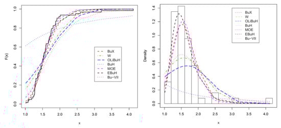
Figure 6. Estimated CDFs (left panel) and PDFs (right panel) of the EBuH distribution and other models for data set I.

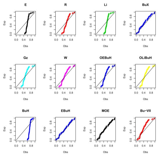
Figure 7. The PP plots of the fitted models for data set I.

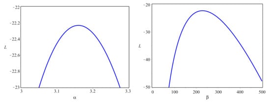
Figure 8. The profile L functions for the EBuH parameters for data set I.

6.2. Data Set II: Discrete Data

Now, we check the flexibility of the DEBuH distribution using a real data set, which refers to final mathematics examination marks of 48 slow space students in the Indian Institute of Technology at Kanpur [19]. The data are: 29, 25, 50, 15, 13, 27, 15, 18, 7, 7, 8, 19, 12, 18, 5, 21, 15, 86, 21, 15, 14, 39, 15, 14, 70, 44, 6, 23, 58, 19, 50, 23, 11, 6, 34, 18, 28, 34, 12, 37, 4, 60, 20, 23, 40, 65, 19, 31. The DEBuH distribution is compared with some discrete rival models called the Geometric (Geo), generalized geometric (GGeo), discrete Pareto (DPar), discrete Lindley (DLi), discrete flexible one parameter [20] (DFI), negative Binomial (NeBi), discrete Burr X type II (DBuX-II), and discrete Burr–Hatke (DBuH).

The parameters of the DEBuH and other competing models are estimated using the ML approach. Table 9 reports the MLEs, SE, and C.I. of the estimates. Table 10 shows the fitting measures of all studied distributions. The estimated CDFs of all considered models are displayed in Figure 9, whereas the PP plots of these discrete models are depicted in Figure 10. The values in Table 10 are supported by the plots in Figure 9 and Figure 10, showing that the new DEBuH model provides a superior fit to the analyzed data. Further, the profile log-likelihood functions of the DEBuH parameters are shown in Figure 11 for data set II.

Table 9. The MLEs, SE, and C.I. of the DEBuH model and other discrete models for data set II.

Model	p			$\mathit{\beta }$
	MLE	SE	C.I.	MLE	SE	C.I.
Geo	$0.9628$	$0.0053$	$[0.953,0.9731]$	−	−	−
GGeo	$0.9262$	$0.0134$	$[0.8997,0.9525]$	$4.7513$	$2.2301$	$[0.3804,9.1223]$
DPar	$0.7243$	$0.0337$	$[0.6583,0.7904]$	−	−	−
DLi	$0.9294$	$0.0069$	$[0.9158,0.9430]$	−	−	−
DFI	$0.9709$	$0.0036$	$[0.9639,0.9781]$	−	−	−
NeBi	$0.9137$	$0.01847$	$[0.8775,0.9499]$	$2.4447$	$0.5219$	$[1.4218,3.4676]$
DBuX-II	$0.9757$	$0.0604$	$[0.8573,1]$	$13.3408$	$33.5855$	$[0,79.1671]$
DBuH	$0.9990$	$0.0046$	$[0.9901,1]$	−	−	−
DEBuH	$0.9693$	$0.0085$	$[0.9527,0.9858]$	$27.6957$	$5.1760$	$[17.5509,7.8406]$

Table 10. Fitting measures of the DEBuH model and other discrete models for data set II.

Model	Fitting Measures
	$-\mathit{L}$	AIC	CAIC	BIC	HQIC	K-S	p-Value
Geo	$205.1110$	$412.2221$	$412.3090$	$414.0933$	$412.9292$	$0.2223$	$0.0174$
GGeo	$200.1725$	$404.3451$	$404.6118$	$408.0875$	$405.7593$	$0.1583$	$0.0962$
DPar	$251.1808$	$504.3617$	$504.4486$	$506.2329$	$505.0688$	$0.4469$	$0.0000$
DLi	$198.2620$	$398.5239$	$398.6109$	$400.3951$	$399.2310$	$0.1048$	$0.6676$
DFI	$202.5758$	$407.1516$	$407.2386$	$409.0228$	$407.8588$	$0.1892$	$0.0642$
NeBi	$197.5218$	$399.0435$	$399.3102$	$402.7859$	$400.4578$	$0.1029$	$0.6810$
DBuX-II	$247.4837$	$498.9674$	$499.2341$	$502.7098$	$500.3817$	$0.4308$	$0.0000$
DBuH	$297.6761$	$597.3523$	$597.4392$	$599.2235$	$598.0594$	$0.8371$	$0.0000$
DEBuH	$196.5340$	$397.0681$	$397.3347$	$400.8105$	$398.4823$	$0.1019$	$0.7008$

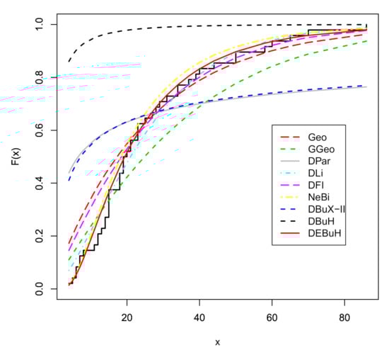
Figure 9. Estimated CDFs of the DEBuH model and other discrete models for data set II.

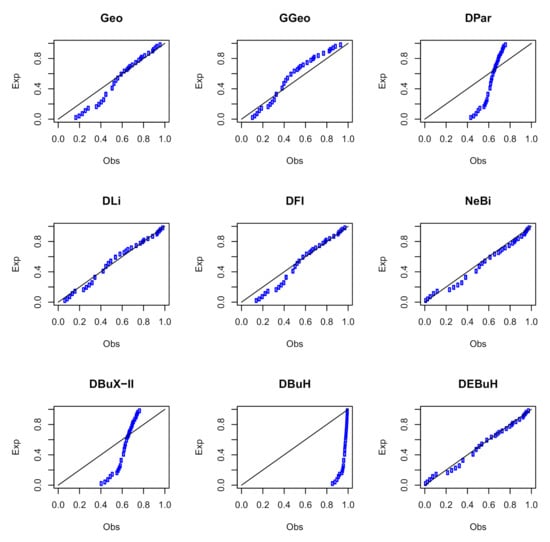
Figure 10. The PP plots of the fitted models for data set II.

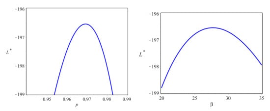
Figure 11. The profile L functions of the DEBuH parameters for data set II.

7. Estimation of the EBuH Parameters under CSALT

In this section, we consider the ML method to estimate the unknown parameters of the EBuH CSALT model. The estimated shape parameter, RF, and MTTF are also obtained under normal use conditions. One real data set is analyzed for illustration purposes. For estimation under CSALT, we need the following assumptions:

1

Let $S_u$ be the stress under normal use condition and $S_1<S_2<...<S_r$ are r increased stress levels, where $S_u<S_1$.

2

A sample size of N identical units is divided into $n_1,n_2,....,n_k$, where $n_j$ units are operated at a fixed stress level $S_j,j=1,...,r.$.

3

The failure times $X_{ij}$, $i=1,2,...,n_j;j=1,2,...,r.$ are independently and identically distributed EBuH random variables with PDF (3).

4

The shape parameter ${\beta }_j,j=1,2,...,r$ is related to the stress level through a log linear relationship, i.e., $log{\beta }_j=v+u{S}_j$, where v and u are two unknown parameters.

7.1. The MLE of the EBuH under the CSALT Model

On the basis of the PDF of the EBuH distribution (3), the likelihood function under CSALT can be expressed as

$$L(\underline{x};\alpha ,v,u)=\prod _{j=1}^r\prod _{i=1}^{n_r}\frac{e^{v+u{S}_j-\alpha x_{ij}}(\alpha x_{ij}+\alpha +1){\left(1+x_{ij}-e^{-\alpha x_{ij}}\right)}^{e^{v+u{S}_j}-1}}{{\left(x_{ij}+1\right)}^{e^{v+u{S}_j}+1}}.$$

(23)

The natural logarithm of the likelihood function (23), say $\ell (\underline{x};\alpha ,v,u)=logL(\underline{x};\alpha ,v,u)$, takes the form

$$\begin{array}{ccc}\hfill \ell (\underline{x};\alpha ,v,u)& =& \sum _{j=1}^r\sum _{i=1}^{n_r}\left[v+u{S}_j-\alpha x_{ij}+log(\alpha x_{ij}+\alpha +1)\right]\hfill \\ & +& \sum _{j=1}^r\sum _{i=1}^{n_r}\left(e^{v+u{S}_j}-1\right)log\left(1+x_{ij}-e^{-\alpha x_{ij}}\right)\hfill \\ & -& \sum _{j=1}^r\sum _{i=1}^{n_r}\left(e^{v+u{S}_j}+1\right)log(x_{ij}+1).\hfill \end{array}$$

(24)

The MLEs of the unknown parameters $u,v$, and $\beta$ can be obtained by maximizing (24) with respect to $u,v$, and $\beta$, or equivalently by solving the following three nonlinear equations:

$$\begin{array}{c}\hfill \sum _{j=1}^r\sum _{i=1}^{n_r}\left[\frac{x_{ij}+1}{\alpha x_{ij}+\alpha +1}-x_{ij}\right]+\sum _{j=1}^r\sum _{i=1}^{n_r}\left(e^{v+u{S}_j}-1\right)\frac{x_{ij}{e}^{-\alpha x_{ij}}}{1+x_{ij}-e^{-\alpha x_{ij}}}=0,\end{array}$$

(25)

$$\begin{array}{c}\hfill N+\sum _{j=1}^r\sum _{i=1}^{n_r}{e}^{v+u{S}_j}log\left(1+x_{ij}-e^{-\alpha x_{ij}}\right)-\sum _{j=1}^r\sum _{i=1}^{n_r}{e}^{v+u{S}_j}log(x_{ij}+1)=0\end{array}$$

(26)

and

$$\begin{array}{c}\hfill N\sum _{j=1}^r{S}_j+\sum _{j=1}^r\sum _{i=1}^{n_r}{S}_j{e}^{v+u{S}_j}log\left(1+x_{ij}-e^{-\alpha x_{ij}}\right)-\sum _{j=1}^r\sum _{i=1}^{n_r}{S}_j{e}^{v+u{S}_j}log(x_{ij}+1)=0.\end{array}$$

(27)

Any numerical technique can be used to solve (25)–(27) to obtain the MLEs of $u,v$, and $\beta$ denoted by $\widehat{u},\widehat{v}$, and $\widehat{\beta }$. Upon obtaining $\widehat{u},\widehat{v}$, and $\widehat{\beta }$, we can obtain the MLE of the shape parameter at stress level j as follows:

$$\begin{array}{c}\hfill {\widehat{\beta }}_j=e^{\widehat{v}+\widehat{u}{S}_j},j=1,...,r.\end{array}$$

(28)

Similarly, the estimated shape parameter, RF at life time $x_0$ and MTTF can be obtained under normal use conditions, respectively, as follows:

$$\begin{array}{c}\hfill {\widehat{\beta }}_u=e^{\widehat{v}+\widehat{u}{S}_u},\end{array}$$

$$\begin{array}{c}\hfill {\widehat{R}}_u\left(x_0\right)=1-{\left(1-\frac{e^{-\widehat{\alpha }{x}_0}}{x_0+1}\right)}^{{\widehat{\beta }}_u}\end{array}$$

and

$$\begin{array}{ccc}\hfill MTT{F}_u& =& {\widehat{\beta }}_u\sum _{j,k=0}^{\infty }{\Theta }_{{\widehat{\beta }}_u}^{(j,k)}\frac{\left(k+2\right)(j+1)(\widehat{\alpha }+1)}{{\left(j+1\right)}^{k+3}{\widehat{\alpha }}^{k+2}}\Gamma \left(k+2\right),\hfill \end{array}$$

7.2. Data Analysis under CSALT

In this subsection, we analyze the data set considered by [21] and analyzed recently by [22]. The data refer to the M00071 white organic light-emitting diode (WOLED) mixed with red, green, and blue colors. The failure times of CSALT samples at $S_1=9.64$ mA and $S_2=17.09$ mA are displayed in Table 4 in [21]. For computational purposes, we subtracted 1500 from each data point at $S_1$ and divided them by 300; we also subtracted 500 from each data point at $S_2$ and divided them by 200. The transformed data are displayed in Table 11. The MLEs are obtained and used to check the validity of the EBuH distribution to fit these data.

Table 11. WOLED data, K-S statistic, and the corresponding p-value.

Stress Level	Failure Data					K-S Distance (p-Value)
$S_1=9.64$ mA	0.638	1.949	2.001	2.915	3.042	0.3009(0.3255)
	3.620	3.738	3.935	4.560	4.598
$S_2=17.09$ mA	0.507	0.949	0.986	1.083	1.428	0.1744(0.9213)
	1.772	1.947	3.079	3.156	3.757

For this purpose, the K-S distance and the corresponding p-value are obtained for each stress level and displayed in Table 11. It is observed from Table 11 that the EBuH distribution provides acceptable fit to the CSALT data. Figure 12 presents the empirical and the estimated EBuH CDF for the two stress levels, indicating that the EBuH distribution is a good choice for modeling this data set. The different estimates of the unknown parameters and MTTF at each stress level, estimated shape parameter, and MTTF at normal use conditions are given by $\widehat{\alpha }=0.350$, $\widehat{v}=4.157$, $\widehat{u}=-0.173$, $\widehat{{\beta }_1}=12.395$, $\widehat{{\beta }_2}=3.302$, $\widehat{{\beta }_u}=22.581$, $\widehat{MTT{F}_1}=4.389$, $\widehat{MTT{F}_2}=2.376$, and $\widehat{MTT{F}_u}=5.476$.

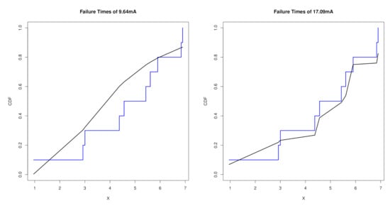
Figure 12. The empirical and estimated CDFs of the EBuH distribution for the two stress levels.

In addition, the estimated RFs for some selected values, $x_0=1,2,3$, at normal use conditions are given by $\widehat{R_u}\left(1\right)=1.000$, $\widehat{R_u}\left(2\right)=0.873$, and $\widehat{R_u}\left(3\right)=0.485$. From these results we conclude that the MTTF decreases as the stress level increases; this is due to the fact that at higher levels of stress the products will fail more quickly. Additionally, it is observed that the MTTF at the normal use condition is higher than those at higher levels of stress. Finally, we can see that the estimated reliability at different mission times decreases as the mission time increases.

8. Conclusions

In this article, we proposed a new form of the Burr–Hatke distribution, called exponentiated Burr–Hatke (EBuH) distribution, that provides more accuracy and flexibility in modeling real data. The discrete version of the new EBuH model is also derived to introduce the discrete exponentiated Burr–Hatke (DEBuH) distribution. The hazard rate and density functions of the EBuH distribution are addressed analytically, and they can be decreasing or unimodal shaped. Furthermore, we studied the shape properties for the reversed hazard rate and odds functions of the EBuH distribution. The reversed hazard function is deceasing for all $\alpha ,\beta >0$, whereas the odds function can be either increasing or bathtub-shaped. Some of the basic reliability properties of the EBuH distribution are derived. The parameters of the EBuH distribution are estimated using several estimation approaches. The behaviors of these estimators are assessed via simulation results. The importance of the EBuH and DEBuH distributions is illustrated empirically using two real-life datasets. It is shown that the two distributions have superior fits compared to other competing models. Additionally, the maximum likelihood approach is adopted to estimate the EBuH parameters under constant-stress accelerated life tests, and a real data set is analyzed to validate our results.

References

- Lehmann, E.L. The power of rank tests. Ann. Math. Stat. 1952, 24, 23–43. [Google Scholar] [CrossRef]
- Mudholkar, G.S.; Srivastava, D.K. Exponentiated Weibull family for analyzing bathtub failure-rate data. IEEE Trans. Reliab. 1993, 42, 299–302. [Google Scholar] [CrossRef]
- Gupta, R.C.; Gupta, P.L.; Gupta, R.D. Modeling failure time data by Lehmann alternatives. Commun. Stat. Theory Methods 1998, 27, 887–904. [Google Scholar] [CrossRef]
- Nadarajah, S.; Kotz, S. The exponentiated type distributions. Acta Appl. Math. 2006, 92, 97–111. [Google Scholar] [CrossRef]
- Aryal, G.; Elbatal, I. On the exponentiated generalized modified Weibull distribution. Commun. Stat. Appl. Methods 2015, 22, 333–348. [Google Scholar] [CrossRef] [Green Version]
- Afify, A.Z.; Yousof, H.M.; Hamedani, G.G.; Aryal, G. The exponentiated Weibull-Pareto distribution with application. J. Stat. Theory Appl. 2016, 15, 328–346. [Google Scholar] [CrossRef] [Green Version]
- Cordeiro, G.M.; Afify, A.Z.; Yousof, H.M.; Pescim, R.R.; Aryal, G.R. The exponentiated Weibull-H family of distributions: Theory and Applications. Mediterr. J. Math. 2017, 14, 155. [Google Scholar] [CrossRef]
- Eliwa, M.S.; El-Morshedy, M.; Ali, S. Exponentiated odd Chen-G family of distributions: Statistical properties, Bayesian and non-Bayesian estimation with applications. J. Appl. Stat. 2020, 48, 1–27. [Google Scholar] [CrossRef]
- El-Morshedy, M.; Eliwa, M.S.; Altun, E. Discrete Burr-Hatke distribution with properties, estimation methods and regression model. IEEE Access 2020, 8, 74359–74370. [Google Scholar] [CrossRef]
- Al-Babtain, A.A.; Ahmed, A.H.N.; Afify, A.Z. A new discrete analog of the continuous Lindley distribution, with reliability applications. Entropy 2020, 22, 603. [Google Scholar] [CrossRef]
- Aljohani, H.M.; Akdoğan, Y.; Cordeiro, G.M.; Afify, A.Z. The uniform Poisson–Ailamujia distribution: Actuarial measures and applications in biological science. Symmetry 2021, 13, 1258. [Google Scholar] [CrossRef]
- Almazah, M.M.A.; Erbayram, T.; Akdoğan, Y.; ALSobhi, M.M.; Afify, A.Z. A new extended geometric distribution: Properties, regression model, and actuarial applications. Mathematics 2021, 9, 1336. [Google Scholar] [CrossRef]
- Maniu, A.I.; Voda, V.G. Generalized Burr-Hatke equation as generator of a homogaphic failure rate. J. Appl. Quant. Methods 2008, 3, 215–222. [Google Scholar]
- Glaser, R.E. Bathtub and related failure rate characterizations. J. Am. Stat. Assoc. 1980, 75, 667–672. [Google Scholar] [CrossRef]
- Lando, T.; Arab, I.; Oliveira, P.E. Second-order stochastic comparisons of order statistics. Statistics 2021. [Google Scholar] [CrossRef]
- Mahmoud, M.R.; Mandouh, R.M. On the transmuted Fréchet distribution. J. Appl. Sci. Res. 2013, 9, 5553–5561. [Google Scholar]
- Raqab, M.Z.; Kundu, D. Burr type X distribution: Revisited. J. Probab. Stat. Sci. 2006, 4, 179–193. [Google Scholar]
- Marshall, A.W.; Olkin, I. A new method for adding a parameter to a family of distributions with application to the exponential and Weibull families. Biometrika 1997, 84, 641–652. [Google Scholar] [CrossRef]
- Gupta, R.D.; Kundu, D. A new class of weighted exponential distributions. Statistics 2009, 43, 621–634. [Google Scholar] [CrossRef]
- Eliwa, M.S.; El-Morshedy, M. A one-parameter discrete distribution for over-dispersed data: Statistical and reliability properties with applications. J. Appl. Stat. 2021. [Google Scholar] [CrossRef]
- Zhang, J.; Cheng, G.; Chen, X.; Han, Y.; Zhou, T.; Qiu, Y. Accelerated life test of white OLED based on lognormal distribution. Indian J. Pure Appl. Phys. 2014, 52, 671–677. [Google Scholar]
- Lin, C.; Hsu, Y.; Lee, S.; Balakrishnan, N. Inference on constant stress accelerated life tests for log-location-scale lifetime distributions with type-I hybrid censoring. J. Stat. Comput. Simul. 2019, 89, 720–749. [Google Scholar] [CrossRef]
Publisher’s Note: MDPI stays neutral with regard to jurisdictional claims in published maps and institutional affiliations. |
© 2021 by the authors. Licensee MDPI, Basel, Switzerland. This article is an open access article distributed under the terms and conditions of the Creative Commons Attribution (CC BY) license (https://creativecommons.org/licenses/by/4.0/).