Residual Probability Function for Dependent Lifetimes

Abstract

In this paper, the residual probability function is applied to analyze the survival probability of two used components relative to each other in the case when their lifetimes are dependent. The expression of the function by copulas has been derived along with some examples of particular copulas. The behaviour of the residual probability function in terms of the underlying dependence is also discussed. The residual probability order is also considered in the dependent case. In the class of Archimedean survival copulas, we prove that the residual probability order implies the usual stochastic order in the reversed direction, and the hazard rate order concludes the residual probability order.

1. Introduction

In statistical survival analysis, various measures have been proposed to predict the future events like the time of the failure of a system or the time of the death of a life span. The hazard rate and the mean residual life of a lifetime unit are two intrinsic characteristics for analyzing lifetime data (see, e.g., Maguluri and Zhang [1], Gupta [2], Klein and Moeschberger [3], Miller Jr. [4] and Cox [5]). In reliability and life testing, the residual life of a unit plays an important role in analysis (cf. Barlow and Proschan [6] and Lai and Xie [7]). In bivariate settings, the role of dependence structures between lifetime random variables is extremely important in applied probability literature (cf. Bassan et al. [8], Finkelstein and Esaulova [9], Pellerey [10] and Mulinacci [11]). Let the random variables X and Y denote the lifetimes of two components of the same system. Usually these random variables are dependent, because they can be affected by the common shock. Suppose further that both components are operating at time $t>0$. In this case, the residual lifetimes of X and Y are given by $(X-t|X>t)$ and $(Y-t|Y>t)$, respectively. Denote by $(X_t,Y_t)=(X-t,Y-t|X>t,Y>t)$ the bivariate residual life of the pair $(X,Y)$ at the point $t>0$ (cf. Mulero and Pellerey [12]). In the case where X and Y and, therefore, $X_t$ and $Y_t$, are independent, it holds that $X_t=(X-t|X>t)$ and $Y_t=(Y-t|Y>t).$ The objective of this research is to investigate the properties of the probability $R(t)=P[X_t>Y_t]$ when X and Y are dependent. Suppose that X and Y are the lifetime of two units. If $X_t$ and $Y_t$ are the lifetimes of the two used units of age $t,$ then the quantity $R(t)$ measures the survival probability of the first used unit relative to the other used unit. In particular, we examine the effect of the dependency of X and Y on the function R of t. In the case when the lifetimes X and Y are independent, this function has been intensively studied—see for example, Zardasht and Asadi [13] and Kayid et al. [14].

The paper is organized as follows. In Section 2, the notions of copulas and stochastic orders are recalled. Section 3 provides main results where the study of the behaviour of $R(t)$ at the disposal of the dependency. Section 4 is dedicated to examine the residual probability order in the dependent case. Finally in Section 5 we conclude the paper with some remarks and further explanations.

2. Preliminary

To evaluate the behaviour of $R(t)$ in the present context, the notion of copula is begged. The latter is a function of dependence which plays a central role for modelling the dependence the components of a random pair have. Specifically, let X and Y be a continuous random variables with joint distribution H and marginal distributions F and G. The copula C associated to the random pair $(X,Y)$ is the distribution of the uniform pair $(U,V)$ such that $U=F(X)$ and $V=G(Y)$. According the Sklar’s theorem, one can express the copula in terms of the joint and marginal distribution functions as follows,

$$C(u,v)=H(F^{-1}(u),G^{-1}(v))\hspace{1em}\mathrm{for} \mathrm{all} (u,v)\in {[0,1]}^2.$$

where $F^{-1}$ and $G^{-1}$ are the inverses of F and G. Notice that the previous formula is equivalent to

$$H(x,y)=C(F(x),G(y))\hspace{1em}\mathrm{for} \mathrm{all} (x,y)\in {\mathbb{R}}^2.$$

Let $\overline{H}$, $\overline{F}$ and $\overline{G}$ denote the survival functions of $(X,Y)$, X and Y, respectively. The previous formula leads to

$$\begin{array}{c}\hfill \overline{H}(x,y)=\widehat{C}(\overline{F}(x),\overline{G}(y))\hspace{1em}\mathrm{for} \mathrm{all} (x,y)\in {\mathbb{R}}^2.\end{array}$$

(1)

The function $\widehat{C}$ is called survival copula. The function $\widehat{C}:[0,1]\times [0,1]\to [0,1]$ is the survival copula associated with the random vector $(X,Y)$ if the identity in (1) holds true. Equivalently, $\widehat{C}$ is the survival copula of $(X,Y)$ with copula function C if

$$\widehat{C}(u,v)=u+v-1+C(1-u,1-v)\hspace{1em}\mathrm{for} \mathrm{all} (u,v)\in {[0,1]}^2.$$

Remark that C and $\widehat{C}$ coincide with independent copula when X and Y are independent, that is,

$$C(u,v)=\widehat{C}(u,v)=\Pi (u,v)=uv\hspace{1em}\mathrm{for} \mathrm{all} (u,v)\in {[0,1]}^2.$$

It is well-known that (see, e.g., Nelsen [15]) for the copula function C and for all $u,v\in [0,1]$,

$$\begin{array}{c}\hfill max(u+v-1,0)\le C(u,v)\le min(u,v).\end{array}$$

(2)

Note that previous bivariate functions $W(u,v)=max(u+v-1,0)$ and $M(u,v)=min(u,v)$ are themselves copulas called Fréchet-Hoeffding bounds. More information about the construction of these bounds is presented in Frechet [16]. For more details on the notion of copulas, we refer the interested reader to Nelsen [15].

One of the well-known class of symmetric survival copulas, is the class of Archimedean survival copulas (cf. Pellerey [10]). A survival copula is said to be Archimedean if it admits the form

$$\begin{array}{c}\hfill \widehat{C}(u,v)=\varphi ({\varphi }^{-1}(u)+{\varphi }^{-1}(v)),u,v\in [0,1],\end{array}$$

(3)

where $\varphi :{\mathbb{R}}^{+}\to [0,1]$ is continuous, positive, decreasing, and convex such that $\varphi (0)=1$ and $\varphi (\infty )=0$. The function ${\varphi }^{-1}$ which is the inverse function of $\varphi$ is called the generator of the Archimedean survival copula $\widehat{C}$. It has been mentioned in Nelsen [15], that a number of standard survival copulas (e.g., Gumbel, Frank, Clayton, and Ali-Mikhail-Haq families) belong to the class of Archimedean survival copulas. Bivariate lifetimes with an Archimedean survival copula are of great interest in reliability and actuarial sciences, and also in many other applied contexts, for instance the dependence structure of frailty models is characterized via the Archimedean survival copulas (see Oakes [17]). The reader can be referred to Genest and Rivest [18,19], Bassan and Spizzichino [20], and references therein, for more aspects of Archimedean survival copulas.

Hereafter, we recall the definitions of certain stochastic orders.

Definition 1.

Let X and Y be two random variables with distribution functions F and G, survival functions $\overline{F}$ and $\overline{G}$ and density functions f and g, respectively. In this paper, we denote the hazard rate of random variables X and Y by $r_X(t)=f(t)/\overline{F}(t)$ and $r_Y(t)=g(t)/\overline{G}(t)$, respectively. X is said to be smaller than Y in the

(i) 

usual stochastic order, denoted by $X{⪯}_{st}Y$, if $\overline{F}(x)\le \overline{G}(x)$ for all x;

(ii) 

hazard rate order, denoted by $X{⪯}_{hr}Y$, if $r_X(t)\ge r_Y(t),$ for all $t\ge 0$, or equivalently if $\overline{G}(x)/\overline{F}(x)$ is increasing in x.

3. Main Results

Expression of $R(t)$ in Dependent Case

In this section, we study the link between probability $R(t)$ and the survival copula of $(X,Y)$. This allows to evaluate the impact of the dependence on $R(t)$. To this end, we first derive a closed-form expression of the probability $R(t)$ in terms of the survival function of $(X,Y)$. Note that $\frac{\partial \overline{H}}{\partial y}(x,x)$ and $\frac{\partial \overline{H}}{\partial x}(x,x)$ are the amounts of the functions $\frac{\partial \overline{H}}{\partial y}$ and $\frac{\partial \overline{H}}{\partial x},$ at the point $(x,x)$, respectively. We will use only differentiable probability distribution functions H and also differentiable copula functions C so that the partial derivatives of H, $\overline{H}$ and C exist and they are continuous.

Theorem 1.

For all $t>0$, the probability $R(t)$ is given by

$$\begin{array}{ccc}\hfill R(t)& =& -\frac{1}{\overline{H}(t,t)}{\int }_t^{\infty }\frac{\partial \overline{H}}{\partial y}(x,x)dx\hfill \end{array}$$

(4)

$$\begin{array}{ccc}\hspace{1em}\hspace{1em}& =& 1+\frac{1}{\overline{H}(t,t)}{\int }_t^{\infty }\frac{\partial \overline{H}}{\partial x}(x,x)dx\hfill \end{array}$$

(5)

Proof. 

One has

$$\begin{array}{ccc}\hfill R(t)& =& P[X_t>Y_t]\hfill \\ & =& P[X>Y|X>t,Y>t]\hfill \\ & =& \frac{{\int }_t^{\infty }P[X>x|Y=x]g(x)dx}{\overline{H}(t,t)}.\hfill \end{array}$$

(6)

For all $x\in \mathbb{R}$ and $y\in S_Y=\{y:g(y)>0\}$

$$\begin{array}{c}\hfill P[X>x|Y=y]=-\frac{1}{g(y)}\frac{\partial \overline{H}}{\partial y}(x,y).\end{array}$$

(7)

The expression (4) is then deduced from (6) and (7). The previous arguments can be easily adapted to derive (5). This can be done by using the relation

$$R(t)=1-\frac{{\int }_t^{\infty }P[Y>x|X=x]dF(x)}{\overline{H}(t,t)}.$$

□

As consequence one can deduced an expression of $R(t)$ in terms of the survival copula and marginal survival functions of $(X,Y)$.

Theorem 2.

For all $t>0$, the probability $R(t)$ is given by

$$\begin{array}{ccc}\hfill R(t)& =& \frac{{\int }_t^{\infty }{\widehat{C}}_{01}(\overline{F}(x),\overline{G}(x))dG(x)}{\widehat{C}(\overline{F}(t),\overline{G}(t))}\hfill \end{array}$$

(8)

$$\begin{array}{ccc}& \hspace{1em}\hspace{1em} =& 1-\frac{{\int }_t^{\infty }{\widehat{C}}_{10}(\overline{F}(x),\overline{G}(x))dF(x)}{\widehat{C}(\overline{F}(t),\overline{G}(t))}\hfill \end{array}$$

(9)

where ${\widehat{C}}_{01}$ and ${\widehat{C}}_{10}$ denote the right and left partial derivative of $\widehat{C}$, namely

$${\widehat{C}}_{01}(u,v)=\frac{\partial \widehat{C}}{\partial v}(u,v)\hspace{1em}\mathit{and}\hspace{1em}{\widehat{C}}_{10}(u,v)=\frac{\partial \widehat{C}}{\partial u}(u,v).$$

Proof. 

From (1), one has, for all $x,y\in \mathbb{R}$

$$\begin{array}{c}\hfill \frac{\partial \overline{H}}{\partial y}(x,x)=-\frac{\partial \widehat{C}}{\partial v}(\overline{F}(x),\overline{G}(x))g(x)=-{\widehat{C}}_{01}(\overline{F}(x),\overline{G}(x))g(x).\end{array}$$

Therefore, (8) and (9) are immediately obtained from (4) and (5). □

Notice that the formulas of $R(t)$ obtained in [13] in dependent case can be deduced from the Formulas (8) and (9). This is immediately obtained from the fact ${\widehat{C}}_{01}(u,v)=u$ and ${\widehat{C}}_{01}(u,v)=v$ when the random variables X and Y are independent. In addition, the previous corollary can be used to analyse the impact of the degree of dependence between the random components X and Y on $R(t)$, as discussed in the next example.

Example 1.

To examine the behaviour of $R(t)$ when random variables X and Y are stochastically dependent, let us suppose that the survival copula of the random pair $(X,Y)$ is a member of the Farlie-Gumbel-Morgenstern family of copulas defined, for all $(u,v)\in {[0,1]}^2$, by

$$\widehat{C}(u,v)=uv+\theta uv(1-u)(1-v),\hspace{1em}\theta \in [-1,1].$$

Clearly, this family of copula includes the independence copula when $\theta =0$ and produces both negative and positive dependence when $\theta \in [-1,0)$ and $\theta \in (0,1]$, respectively. In addition, the partial derivative with respect to the second component of $\widehat{C}(u,v)$ is given by

$${\widehat{C}}_{01}(u,v)=u+\theta u(1-u)(1-2v),(u,v)\in {[0,1]}^2.$$

To analyse the impact of the dependence parameter θ on the probability $R(t)$, let us consider the case when the marginal random variables X and Y are exponentially distributed with survival functions $\overline{F}(x)=e^{-\lambda x}$ and $\overline{G}(x)=e^{-\mu x}$, $x\ge 0$, respectively. By making the substitution $u=\overline{G}$ in (8), one has

$$\begin{array}{ccc}\hfill R_{\theta }(t)& =& \frac{{\int }_0^{\overline{G}(t)}{\widehat{C}}_{01}(\overline{F}\circ {\overline{G}}^{-1}(u),u)du}{\widehat{C}(\overline{F}(t),\overline{G}(t))}\hfill \\ & =& \frac{{\int }_0^{e^{-\mu t}}{\widehat{C}}_{01}(u^{\frac{\lambda }{\mu }},u)du}{\widehat{C}(\overline{F}(t),\overline{G}(t))}\hfill \\ & =& \frac{{\int }_0^{e^{-\mu t}}\{u^{\frac{\lambda }{\mu }}+\theta u^{\frac{\lambda }{\mu }}(1-u^{\frac{\lambda }{\mu }})(1-2u)\}du}{\widehat{C}(\overline{F}(t),\overline{G}(t))}.\hfill \end{array}$$

An explicit form of $R_{\theta }(t)$ is then derived by carrying out the previous integral, that is,

$$\begin{array}{ccc}\hfill R_{\theta }(t)& =& \frac{A(t)+\theta B(t)}{1+\theta D(t)},\hfill \end{array}$$

(10)

with

$$\begin{array}{ccc}\hfill A(t)& =& \frac{\mu }{\lambda +\mu },B(t)=\frac{\mu \{1+e^{-(\lambda +\mu )t}\}}{\lambda +\mu }-\frac{\mu e^{-\lambda t}}{2\lambda +\mu }-\frac{2\mu e^{-\mu t}}{\lambda +2\mu },D(t)=(1-e^{-\lambda t})(1-e^{-\mu t}).\hfill \end{array}$$

Note that $R(t)=\mu /(\lambda +\mu )$ when $\theta =0$. This coincides with the expression of $R(t)$ computed when X and Y are assumed independent. In addition, for fixed $t>0$, one has from (10),

$$\begin{array}{ccc}\hfill \frac{d{R}_{\theta }(t)}{d\theta }& =& \frac{B(t)-A(t)D(t)}{{(1+\theta D(t))}^2}\hfill \\ & =& \frac{\lambda }{(\lambda +\mu ){(1+\theta D(t))}^2}\{\frac{e^{-\lambda t}}{2\lambda +\mu }-\frac{e^{-\mu t}}{\lambda +2\mu }\}.\hfill \end{array}$$

It is easy to check that $\lambda <\mu$ (resp. $\lambda >\mu$) implies $d{R}_{\theta }(t)/d\theta >0$ (resp. $d{R}_{\theta }(t)/d\theta <0$). This means that for any $t>0$, $R_{\theta }(t)$ increases (resp. decreases) in terms of the dependence parameter when $\lambda <\mu$ (resp. $\mu <\lambda$).

Hereafter, we derive bounds on the reliability function $R(t)$ in terms of the diagonal section of the survival copula.

Theorem 3.

Assume that the survival copula $\widehat{C}$ of X and Y is symmetric, that is, $\widehat{C}(u,v)=\widehat{C}(v,u)$, for all $(u,v)\in {[0,1]}^2$. Let ${\delta }_{\widehat{C}}$ be the diagonal section of $\widehat{C}$ defined by ${\delta }_{\widehat{C}}(t)=\widehat{C}(t,t)$ for all $t\in [0,1]$.

(i) 

If $X{⪯}_{st}Y$ then

$$\begin{array}{c}\hfill R(t)\le 1-\frac{{\delta }_{\widehat{C}}(\overline{F}(t))}{2\widehat{C}(\overline{F}(t),\overline{G}(t))}.\end{array}$$

(11)

(ii) 

If $Y{⪯}_{st}X$ then

$$\begin{array}{c}\hfill R(t)\ge \frac{{\delta }_{\widehat{C}}(\overline{G}(t))}{2\widehat{C}(\overline{F}(t),\overline{G}(t))}.\end{array}$$

(12)

Proof. 

(i) It is well known from Theorem 2.2.7 in Nelsen [15] that ${\widehat{C}}_{10}(u,v)$ is an increasing function of v for all u. So, $X{⪯}_{st}Y$ or equivalently $\overline{F}(x)\le \overline{G}(x)$ for all x, implies from (9) that

$$\begin{array}{ccc}\hfill R(t)& \le & 1-\frac{{\int }_t^{\infty }{\widehat{C}}_{10}(\overline{F}(x),\overline{F}(x))dF(x)}{\widehat{C}(\overline{F}(t),\overline{G}(t))}\hfill \\ & =& 1-\frac{{\int }_0^{\overline{F}(t)}{\widehat{C}}_{10}(u,u)du}{\widehat{C}(\overline{F}(t),\overline{G}(t))},\hfill \end{array}$$

(13)

where the last equality is obtained by setting $u=\overline{F}(x)$. Since the copula $\widehat{C}$ is symmetric, then

$${\delta }_{\widehat{C}}^{\prime }(t)=C_{01}(t,t)+C_{10}(t,t)=2C_{10}(t,t).$$

Therefore,

$$\begin{array}{c}\hfill {\int }_0^{\overline{F}(t)}{\widehat{C}}_{10}(u,u)du=\frac{1}{2}{\int }_0^{\overline{F}(t)}{\delta }_{\widehat{C}}^{\prime }(u)du=\frac{1}{2}{\delta }_{\widehat{C}}(\overline{F}(t)).\end{array}$$

(14)

Finally, (11) is deduced from (13) and (14). (ii) Similarly, if $Y{⪯}_{st}X$, then one has from (8)

$$\begin{array}{ccc}\hfill R(t)& \ge & \frac{{\int }_t^{\infty }{\widehat{C}}_{01}(\overline{G}(x),\overline{G}(x))dG(x)}{\widehat{C}(\overline{F}(t),\overline{G}(t))}\hfill \\ & =& \frac{1}{2}\frac{{\int }_0^{\overline{G}(t)}{\delta }_{\widehat{C}}^{\prime }(u)du}{\widehat{C}(\overline{F}(t),\overline{G}(t))}=\frac{{\delta }_{\widehat{C}}(\overline{G}(t))}{2\widehat{C}(\overline{F}(t),\overline{G}(t))}.\hfill \end{array}$$

□

Furthermore, if the survival copula of $(X,Y)$ is Archimedean with generator $\varphi$, then the upper and lower bounds described in (11) and (12) are explicitly expressed in terms of $\varphi$ as follows

$$1-\frac{\varphi [2{\varphi }^{-1}(\overline{F}(t)]}{2\varphi [{\varphi }^{-1}(\overline{F}(t))+{\varphi }^{-1}(\overline{G}(t))]}\hspace{1em}\mathrm{and}\hspace{1em}\frac{\varphi [2{\varphi }^{-1}(\overline{G}(t)]}{2\varphi [{\varphi }^{-1}(\overline{F}(t))+{\varphi }^{-1}(\overline{G}(t))]}.$$

In particular, if the random variables X and Y are independent, that is, the copula of $(X,Y)$ is Archimedean with generator $\varphi (t)=e^{-t}$, $t\ge 0$. In such case, the previous bounds become,

$$1-\frac{{\delta }_{\widehat{C}}(\overline{F}(t))}{2\widehat{C}(\overline{F}(t),\overline{G}(t))}=1-\frac{\overline{F}(t)}{2\overline{G}(t)}\hspace{1em}\mathrm{and}\hspace{1em}\frac{{\delta }_{\widehat{C}}(\overline{G}(t))}{2\widehat{C}(\overline{F}(t),\overline{G}(t))}=\frac{\overline{G}(t)}{2\overline{F}(t)},$$

respectively. The latter coincide with the bounds stated in Theorem 2 in [13].

Remark that the bounds (11) and (12) depend on the survival copulas and the marginal survivals of the random pair $(X,Y)$. However, when the dependence structure induces via the survival copula is unknown, one can use the Fréchet-Hoeffding bounds described in (2) to derive bounds on $R(t)$ which dependent only on the marginal distributions of $(X,Y)$ as stated below.

Corollary 1.

(i) 

If $X{⪯}_{st}Y$ then

$$\begin{array}{c}\hfill R(t)\le 1-\frac{max(2\overline{F}(t)-1,0)}{2\overline{F}(t)}.\end{array}$$

(15)

(ii) 

If $Y{⪯}_{st}X$ then

$$\begin{array}{c}\hfill R(t)\ge \frac{max(2\overline{G}(t)-1,0)}{2\overline{G}(t)}.\end{array}$$

(16)

Proof. 

From (2), one has for every survival copulas $\widehat{C}$, ${\delta }_{\widehat{C}}(u)\ge max(2u-1,0)$ and $\widehat{C}(u,v)\le min(u,v)$ for all $u,v\in [0,1]$. We deduce from (11) that if $X{⪯}_{st}Y$, that is, $\overline{F}(x)\le \overline{G}(x)$ for all x, then

$$R(t)\le 1-\frac{{\delta }_{\widehat{C}}(\overline{F}(t))}{2\widehat{C}(\overline{F}(t),\overline{G}(t))}\le 1-\frac{max(2\overline{F}(t))-1,0)}{2min[\overline{F}(t),\overline{G}(t)]}=1-\frac{max(2\overline{F}(t))-1,0)}{2\overline{F}(t)},$$

which ensures the inequality (15). Similar arguments imply (16). □

Hereafter, we discuss the monotonicity of the survival function $R(t)$.

Theorem 4.

Let $\rho (t)=\frac{\partial \overline{H}}{\partial y}(t,t)/\frac{\partial \overline{H}}{\partial x}(t,t)$ for all $t\in \mathcal{S}=\{t:\frac{\partial \overline{H}}{\partial x}(t,t)>0\}$.

1. 

$R(t)$ is increasing (decreasing) if $\rho (t)$ is increasing (decreasing) for all $t\in \mathcal{S}$.

2. 

$R(t)$ is constant if $\rho (t)$ is constant for all $t\in \mathcal{S}$.

Proof. 

Let $f_Z$ be the density function of the random variable $Z=min(X,Y)$. Clearly,

$$f_Z(t)=-\frac{\partial \overline{H}}{\partial x}(t,t)-\frac{\partial \overline{H}}{\partial y}(t,t).$$

So, one has from (4),

$$R(t)=\frac{{\int }_t^{\infty }{f}_Z(x)w(x)dx}{{\int }_t^{\infty }{f}_Z(x)dx},$$

where

$$w(t)=\frac{\rho (t)}{1+\rho (t)}.$$

Therefore,

$$\begin{array}{c}\hfill R^{\prime }(t)=\frac{f_Z(t){\int }_t^{\infty }{f}_Z(x)[w(x)-w(t)]dx}{{\left({\int }_t^{\infty }{f}_Z(x)dx\right)}^2},\end{array}$$

(17)

which implies that $R^{\prime }(t)\ge 0$ ($R^{\prime }(t)\le 0$) if $w(t)$ is increasing (decreasing). The part (1) is then deduced from the fact that $w(t)$ and $\rho (t)$ possess the same shape behaviour, since the function $x/(1+x)$ is increasing in $x>0$. To show the part (2), suppose that $\rho (t)$ is constant which implies that $w(t)$ is also constant. It follows from (17) that $R^{\prime }(t)=0$, $t\in \mathcal{S}$, that is, $R(t)$ is constant in $\mathcal{S}$. To prove the converse of (2), first observe from (17) that

$$\begin{array}{c}\hfill R^{\prime }(t)=r_Z(t)[R(t)-w(t)],\hspace{1em}t\in \mathcal{S},\end{array}$$

where $r_Z(t)=f_Z(t)/{\int }_t^{\infty }{f}_Z(x)dx$ is the hazard rate corresponding to Z. It follows from the above formula that $R(t)$ constant leads to $\rho (t)$ is constant over $\mathcal{S}$ which completes the proof. □

Remark that if X and Y are independent, one has for all $t\in \mathcal{S}=\{t:\frac{\partial \overline{H}}{\partial x}(t,t)>0\}$,

$$\rho (t)=\frac{\partial \overline{H}}{\partial y}(t,t)/\frac{\partial \overline{H}}{\partial x}(t,t)=\frac{r_Y(t)}{r_X(t)}.$$

In that case, the statements (1) and (2) of the Theorem 4 reduce to those of Theorem 1 in [13].

In what follows, we discuss the behaviour of $R(t)$ when the underlying copula of $(X,Y)$ is Archimedean.

Theorem 5.

Assume that the random variables X and Y are connected with an Archimedean copula with generator ϕ.

1. 

Assume that $X{⪯}_{hr}({⪰}_{hr})Y$ and $\frac{\varphi (u)}{{\varphi }^{\prime }(u)}$ is increasing (decreasing) and convex (concave), then $r_Y(t)/r_X(t)$ is increasing implies $R(t)$ is increasing.

2. 

Assume that $Y{⪯}_{hr}({⪰}_{hr})X$ and $\frac{\varphi (u)}{{\varphi }^{\prime }(u)}$ is increasing (decreasing) and convex (concave), then $r_Y(t)/r_X(t)$ is decreasing implies $R(t)$ is decreasing.

Proof. 

From, one has

$$\begin{array}{c}\hfill \rho (t)=\frac{\partial \overline{H}}{\partial y}(t,t)/\frac{\partial \overline{H}}{\partial x}(t,t)=\frac{{\varphi }^{\prime }[{\varphi }^{-1}(\overline{F}(t))]}{{\varphi }^{\prime }[{\varphi }^{-1}(\overline{G}(t))]}\times \frac{\overline{G}(t)}{\overline{F}(t)}\times \frac{r_Y(t)}{r_X(t)}.\end{array}$$

The latter is increasing if $\mathcal{K}(t)=\{{\varphi }^{\prime }[{\varphi }^{-1}(\overline{F}(t))]/\overline{F}(t))\}/\{{\varphi }^{\prime }[{\varphi }^{-1}(\overline{G}(t))]/\overline{G}(t))\}$ is increasing. Therefore, $\mathcal{K}{(t)}^{\prime }\ge 0$ if

$$\begin{array}{ccc}\hfill & & \frac{{\left\{{\varphi }^{\prime }\left[{\varphi }^{-1}\left(\overline{F}\left(t\right)\right)\right]\right\}}^2-\varphi \left[{\varphi }^{-1}\left(\overline{F}\left(t\right)\right)\right]{\varphi }^{\prime \prime }\left[{\varphi }^{-1}\left(\overline{F}\left(t\right)\right)\right]}{{\left\{{\varphi }^{\prime }\left[{\varphi }^{-1}\left(\overline{F}\left(t\right)\right)\right]\right\}}^2}{r}_X(t)\hfill \\ & -& \frac{{\left\{{\varphi }^{\prime }\left[{\varphi }^{-1}\left(\overline{G}\left(t\right)\right)\right]\right\}}^2-\varphi \left[{\varphi }^{-1}\left(\overline{G}\left(t\right)\right)\right]{\varphi }^{\prime \prime }\left[{\varphi }^{-1}\left(\overline{G}\left(t\right)\right)\right]}{{\left\{{\varphi }^{\prime }\left[{\varphi }^{-1}\left(\overline{G}\left(t\right)\right)\right]\right\}}^2}{r}_Y(t)\ge 0.\hfill \end{array}$$

(18)

Remark that

$$\frac{{\left\{{\varphi }^{\prime }[{\varphi }^{-1}(\overline{F}(t))]\right\}}^2-\varphi [{\varphi }^{-1}(\overline{F}(t))]{\varphi }^{″}[{\varphi }^{-1}(\overline{F}(t))]}{{\left\{{\varphi }^{\prime }[{\varphi }^{-1}(\overline{F}(t))]\right\}}^2}=m[{\varphi }^{-1}(\overline{F}(t))]$$

where $m(u)={\left(\frac{\varphi (u)}{{\varphi }^{\prime }(u)}\right)}^{\prime }$ which is positive and increasing if $\frac{\varphi (u)}{{\varphi }^{\prime }(u)}$ is increasing and convex. In addition, $X{⪯}_{hr}Y$ implies $r_Y(t)\le r_X(t)$ and $\overline{F}(t)\le \overline{G}(t)$. Consequently,

$$0\le m([{\varphi }^{-1}(\overline{G}(t))])\le m([{\varphi }^{-1}(\overline{F}(t))])\hspace{1em}\mathrm{and}\hspace{1em}0\le r_Y(t)\le r_X(t).$$

Thus (18) is satisfied, which shows the first part of (1). Suppose that $\frac{\varphi (u)}{{\varphi }^{\prime }(u)}$ is decreasing and concave, so $\tilde{m}(t)=-m(t)$ is positive and increasing. It follows that $Y{⪯}_{hr}X$ implies

$$\tilde{m}([{\varphi }^{-1}(\overline{G}(t))])r_Y(t)-\tilde{m}([{\varphi }^{-1}(\overline{F}(t))])r_X(t)\ge 0.$$

Therefore, (18) is verified which completes the proof of the second part of (1). Similar arguments lead to (2), hence the proof is omitted. □

Example 2.

To illustrate the Theorem 5, assume that the copula of the random pair $(X,Y)$ is Archimedean $C_{\varphi }$ with generator ϕ. The conditions on the generator ϕ indicated in Theorem 5 hold for most of the Archimedean copulas mentioned in Nelsen [15]. For example, suppose that $C_{\varphi }$ is Gumbel copula with generator

$${\varphi }_{\theta }(t)=e^{-t^{\frac{1}{\theta }}},\hspace{1em}t>0\hspace{1em}\theta \ge 1.$$

This model generate only the positive dependence. Furthermore, standard calculations show that

$${\left(\frac{{\varphi }_{\theta }(t)}{{\varphi }_{\theta }^{\prime }(t)}\right)}^{\prime }=(1-\theta )t^{-\frac{1}{\theta }}\hspace{1em}\mathrm{and}\hspace{1em}{\left(\frac{{\varphi }_{\theta }(t)}{{\varphi }_{\theta }^{\prime }(t)}\right)}^{″}=\frac{1}{\theta }(\theta -1)t^{1-\frac{1}{\theta }}$$

which implies that ${\varphi }_{\theta }/{\varphi }_{\theta }^{\prime }$ is decreasing and convex for any $\theta \ge 1$. Let us now consider Frank copula which generates both positive and negative dependence. This copula is characterized by the following generator

$${\varphi }_{\theta }(t)=-\frac{1}{\theta }ln[f_{\theta }(t)],\hspace{1em}\theta \in \mathbb{R},\hspace{1em}\theta \ne 0,$$

where $f_{\theta }(t)=1+e^{-t}(e^{-\theta }-1)$, $t>0$. Elementary calculations show that

$$\frac{{\varphi }_{\theta }(t)}{{\varphi }_{\theta }^{\prime }(t)}=\frac{f_{\theta }(t)ln\{f_{\theta }(t)\}}{1-f_{\theta }(t)},\hspace{1em}t>0.$$

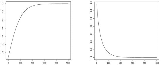
It is easy to check numerically that ${\varphi }_{\theta }/{\varphi }_{\theta }^{\prime }$ is decreasing (increasing) and convex (concave) if $\theta >0$ ($\theta <0$). For example, the next Figure 1 displays the graphics of the function $\frac{{\varphi }_{\theta }(t)}{{\varphi }_{\theta }^{\prime }(t)}$ for $\theta =-2$ and $\theta =2$, respectively. These graphics suggest that $\frac{{\varphi }_{\theta }(t)}{{\varphi }_{\theta }^{\prime }(t)}$ is decreasing (increasing) and convex (concave) for $\theta =-2$ ($\theta =2$).

4. Probability Ordering of Residual Lifetimes in Dependent Case

Stochastic comparison of lifetime random variables according to their residual life has attracted the attention of many researchers during the past decades (cf. Bassan and Spizzichino [21], Belzunce et al. [22], Misra et al. [23], Kayid [24] and Gupta et al. [25]). Mi [26] introduced the concept of probability ordering for comparison of lifetimes of systems as follows. The variable X is said to be less than Y in probability ordering (denoted by $X{⪯}_{pr}Y$) whenever $P(X>Y)\le 1/2$. To affect the probability ordering of the lifetime units by the age of them, Zardasht and Asadi [13] proposed the residual probability ordering, denoted by $X{⪯}_{rpr}Y,$ when $R(t)\le 1/2$ for all $t\ge 0,$ where X and Y are assumed to be independent. Recently, Kayid et al. [14] conducted a further study of the residual probability order and its related aging classes. Here, the residual probability order in the dependent case is considered. Formally, we say X is smaller than Y in the residual probability order in dependent case, denoted by $X{⪯}_{rpr}^{(d)}Y,$ if $R(t)\le 1/2$ for all $t\ge 0$ where X and Y can be dependent.

The following result presents some equivalent conditions for the order ${⪯}_{rpr}^{(d)}.$

Theorem 6.

Let $(X,Y)$ be a pair of non-negative random variables with joint survival function $\overline{H}$ and joint probability density function $h.$ Then the following assertions are equivalent.

(i) 

$X{⪯}_{rpr}^{(d)}Y.$

(ii) 

$P(X>Y>t)\le P(Y\ge X>t),$ for all $t\ge 0.$

(iii) 

${\int }_t^{\infty }{\int }_x^{\infty }(h(x,y)-h(y,x))dydx\ge 0,$ for all $t\ge 0.$

(iv) 

${\int }_t^{\infty }(\frac{\partial }{\partial y}\overline{H}(x,x)-\frac{\partial }{\partial x}\overline{H}(x,x))dx\ge 0,$ for all $t\ge 0.$

Proof. 

To demonstrate that $(i)$ and $(ii)$ are equivalent, observe first that

$$\begin{array}{ccc}\hfill P(X>t,Y>t)& =& P(X>t,Y>t,X>Y)+P(X>t,Y>t,X\le Y)\hfill \\ & =& P(X>Y>t)+P(Y\ge X>t),\mathrm{for} \mathrm{all} t\ge 0.\hfill \end{array}$$

Therefore,

$$\begin{array}{ccc}\hfill R(t)& =& \frac{P(X>Y>t)}{P(X>t,Y>t)}\hfill \\ & =& \frac{P(X>Y>t)}{P(X>Y>t)+P(Y\ge X>t)},\mathrm{for} \mathrm{all} t\ge 0,\hfill \end{array}$$

from which $R(t)\le 1/2,$ for all $t\ge 0,$ if and only if, $P(X>Y>t)\le P(Y\ge X>t),$ for all $t\ge 0.$ The equivalence between (i) and $(iii)$ is shown from (ii), by noting that

$$\begin{array}{ccc}\hfill P(X>Y>t)& =& {\int }_t^{\infty }{\int }_x^{\infty }h(y,x)dydx,\hfill \end{array}$$

and

$$\begin{array}{ccc}\hfill P(Y\ge X>t)& =& {\int }_t^{\infty }{\int }_x^{\infty }h(x,y)dydx.\hfill \end{array}$$

Likewise, we can deduce from $(iii)$ that $(iv)$ and $(i)$ are equivalent because

$$\begin{array}{ccc}\hfill {\int }_t^{\infty }{\int }_x^{\infty }h(y,x)dydx& =& {\int }_t^{\infty }-\frac{\partial }{\partial y}\overline{H}(x,x)dx,\hfill \end{array}$$

and

$$\begin{array}{ccc}\hfill {\int }_t^{\infty }{\int }_x^{\infty }h(x,y)dydx& =& {\int }_t^{\infty }-\frac{\partial }{\partial x}\overline{H}(x,x)dx.\hfill \end{array}$$

 □

Theorem 7.

Let $(X,Y)$ be a pair of non-negative random variables sharing the Archimedean survival copulas as in (3), and let X and Y have absolutely continuous distributions, and ϕ is differentiable. Suppose that the limit of ${\varphi }^{-1}(\overline{F}(s))-{\varphi }^{-1}(\overline{G}(s))$ as $s\to \infty$ exists and is negative. Then $X{⪯}_{rpr}^{(d)}Y$ implies $X{⪰}_{st}Y.$

Proof. 

Note that from (1) and (3), $(X,Y)$ has joint survival function

$$\begin{array}{c}\hfill \overline{H}(x,y)=\varphi ({\varphi }^{-1}(\overline{F}(x))+{\varphi }^{-1}(\overline{G}(y))),x,y\ge 0,\end{array}$$

from which we get

$$\begin{array}{ccc}\hfill -\frac{\partial }{\partial x}\overline{H}(x,x)& =& f(x)\frac{-{\varphi }^{\prime }({\varphi }^{-1}(\overline{F}(x))+{\varphi }^{-1}(\overline{G}(x)))}{-{\varphi }^{\prime }({\varphi }^{-1}(\overline{F}(x)))},x\ge 0,\hfill \end{array}$$

and

$$\begin{array}{ccc}\hfill -\frac{\partial }{\partial y}\overline{H}(x,x)& =& g(x)\frac{-{\varphi }^{\prime }({\varphi }^{-1}(\overline{F}(x))+{\varphi }^{-1}(\overline{G}(x)))}{-{\varphi }^{\prime }({\varphi }^{-1}(\overline{G}(x)))},x\ge 0.\hfill \end{array}$$

Thus, by Theorem 6 (iv), $X{⪯}_{rpr}^{(d)}Y$ holds if, and only if, for all $t\ge 0,$

$${\int }_t^{\infty }-{\varphi }^{\prime }({\varphi }^{-1}(\overline{F}(x))+{\varphi }^{-1}(\overline{G}(x)))\{\frac{f(x)}{-{\varphi }^{\prime }({\varphi }^{-1}(\overline{F}(x)))}-\frac{g(x)}{-{\varphi }^{\prime }({\varphi }^{-1}(\overline{G}(x)))}\}dx\ge 0,$$

(19)

which by Lemma 7.1 (b) of Barlow and Proschan [6] implies that

$${\int }_t^{\infty }(\frac{f(x)}{-{\varphi }^{\prime }({\varphi }^{-1}(\overline{F}(x)))}-\frac{g(x)}{-{\varphi }^{\prime }({\varphi }^{-1}(\overline{G}(x)))})dx\ge 0,\forall t\ge 0,$$

(20)

because $1/(-{\varphi }^{\prime }({\varphi }^{-1}(\overline{F}(x))+{\varphi }^{-1}(\overline{G}(x))))$ is positive and also increasing in $x\ge 0$. Now, let us observe that for all $s>t\ge 0$

$$\begin{array}{ccc}\hfill {\int }_t^s\frac{f(x)}{-{\varphi }^{\prime }({\varphi }^{-1}(\overline{F}(x)))}dx& =& {\varphi }^{-1}(\overline{F}(s))-{\varphi }^{-1}(\overline{F}(t)),\hfill \end{array}$$

and that

$$\begin{array}{ccc}\hfill {\int }_t^s\frac{g(x)}{-{\varphi }^{\prime }({\varphi }^{-1}(\overline{G}(x)))}dx& =& {\varphi }^{-1}(\overline{G}(s))-{\varphi }^{-1}(\overline{G}(t)).\hfill \end{array}$$

Hence, (20) is equivalent to ${\varphi }^{-1}(\overline{F}(t))-{\varphi }^{-1}(\overline{G}(t))\le {lim}_{s\to \infty }({\varphi }^{-1}(\overline{F}(s))-{\varphi }^{-1}(\overline{G}(s))),$ for all $t\ge 0.$ By assumption, it concludes that ${\varphi }^{-1}(\overline{F}(t))\le {\varphi }^{-1}(\overline{G}(t))$ for all $t\ge 0$. Since, ${\varphi }^{-1}$ is a decreasing function, thus $\overline{G}(t)\le \overline{F}(t),$ for all $t\ge 0.$ That is, $X{⪰}_{st}Y.$ □

Theorem 8.

Let $(X,Y)$ be a pair of non-negative random variables sharing the Archimedean survival copulas as in (3), and let X and Y have absolutely continuous distributions, and ϕ is differentiable. If ϕ is, a log-convex function, then $X{⪯}_{hr}Y$ implies $X{⪯}_{rpr}^{(d)}Y$.

Proof. 

Let $r_X(x)=f(x)/\overline{F}(x)$ and $r_Y(x)=g(x)/\overline{G}(x)$, $x\in \mathbb{R}$, be the hazard rate of X and Y, respectively. Assume that $X{⪯}_{hr}Y$, then $r_X(x)\ge r_Y(x)$ and $\overline{F}(x)\le \overline{G}(x)$ for all $x\in \mathbb{R}$. Furthermore, the function $-\varphi ({\varphi }^{-1}(t))/{\varphi }^{\prime }({\varphi }^{-1}(t))$ is positive and decreasing in $t>0$, if $\varphi$ is a log-convex function. Consequently,

$$0\le \frac{\varphi ({\varphi }^{-1}(\overline{G}(x)))}{-{\varphi }^{\prime }({\varphi }^{-1}(\overline{G}(x)))}\le \frac{\varphi ({\varphi }^{-1}(\overline{F}(x)))}{-{\varphi }^{\prime }({\varphi }^{-1}(\overline{F}(x)))}\hspace{1em}\mathrm{and}\hspace{1em}0\le r_Y(x)\le r_X(x)$$

which imply

$$\begin{array}{ccc}& & \frac{f(x)}{-{\varphi }^{\prime }({\varphi }^{-1}(\overline{F}(x)))}-\frac{g(x)}{-{\varphi }^{\prime }({\varphi }^{-1}(\overline{G}(x)))}\hfill \\ & =& \frac{\varphi ({\varphi }^{-1}(\overline{F}(x)))}{-{\varphi }^{\prime }({\varphi }^{-1}(\overline{F}(x)))}{r}_X(x)-\frac{\varphi ({\varphi }^{-1}(\overline{G}(x)))}{-{\varphi }^{\prime }({\varphi }^{-1}(\overline{G}(x)))}{r}_Y(x)\ge 0.\hfill \end{array}$$

This in turn ensures that (19) is satisfied, that is, $X{⪯}_{rpr}^{(d)}Y$. □

Note that if X and Y are independent, the generator of the copula associated to $(X,Y)$ is the form $\varphi (t)=e^{-t}$, $t\ge 0$ which is a log-convex function. In this situation, the result of previous Theorem is valid in the dependence case, as indicated in Theorem 6 in [13]. More generally, the implication stated in the Theorem 8 is still true when the random variables X and Y are positively dependent. To see this, let us recall an important notion of association defined as follows: Y is left tail decreasing in X, denoted LTD$(X|Y)$, if $P[Y\le y|X\le x]$ is a decreasing function of x for all y. It is well known that this concept of association characterizes the positive dependence. In particular, if the copula of $(X,Y)$ is Archimedean with generator $\varphi$, then LTD$(X|Y)$ is equivalent to $\varphi$ is a log-convex function.

5. Conclusions

The residual probability function as a measure of relative survival probability for random dependent lifetimes was considered. The class of Archimedean copulas as a typical dependence structure was applied to examine some interesting examples. Bounds on the survival probability of the first used unit relative to the other used unit were derived in terms of underlying copula diagonal section. These bounds were reduced for unknown copulas through the Fréchet-Hoeffding bounds. The monotonicity behavior of the residual probability function in terms of the age of the two units with dependent lifetimes is a useful observation to detect the unit which fails faster. This property was studied in Theorem 5 with some conditions on the generator of the Archimedean copula and also further ordering relations of distributions of lifetimes of units. The residual probability ordering was introduced and studied before closing the paper. This stochastic ordering property means that the rate of survival of one unit is better (worse) that the other during the time which may be useful for example to recognize better product with high survival between two products with dependent lifetimes.

References

- Maguluri, G.; Zhang, C.H. Estimation in the mean residual life regression model. J. R. Stat. Soc. Ser. B Methodol. 1994, 56, 477–489. [Google Scholar] [CrossRef]
- Gupta, R.C. On the mean residual life function in survival studies. In Statistical Distributions in Scientific Work; Springer: Dordrecht, The Netherlands, 1981; pp. 327–334. [Google Scholar]
- Klein, J.P.; Moeschberger, M.L. Survival Analysis: Techniques for Censored and Truncated Data; Springer Science & Business Media: New York, NY, USA, 2005. [Google Scholar]
- Miller, R.G., Jr. Survival Analysis; John Wiley & Sons: Hoboken, NJ, USA, 2011; Volume 66. [Google Scholar]
- Cox, D.R. Analysis of Survival Data; Routledge: London, UK, 2018. [Google Scholar]
- Barlow, R.E.; Proschan, F. Statistical Theory of Reliability and Life Testing: Probability Models; Florida State University: Tallahassee, FL, USA, 1975. [Google Scholar]
- Lai, C.D.; Xie, M. Stochastic Ageing and Dependence for Reliability; Springer Science & Business Media: New York, NY, USA, 2006. [Google Scholar]
- Bassan, B.; Kochar, S.; Spizzichino, F. Some bivariate notions of IFR and DMRL and related properties. J. Appl. Probab. 2002, 39, 533–544. [Google Scholar] [CrossRef][Green Version]
- Finkelstein, M.; Esaulova, V. On the weak IFR aging of bivariate lifetime distributions. Appl. Stoch. Model. Bus. Ind. 2005, 21, 265–272. [Google Scholar] [CrossRef]
- Pellerey, F. On univariate and bivariate aging for dependent lifetimes with Archimedean survival copulas. Kybernetika 2008, 44, 795–806. [Google Scholar]
- Mulinacci, S. Archimedean-based Marshall-Olkin Distributions and Related Dependence Structures. Methodol. Comput. Appl. Probab. 2018, 20, 205–236. [Google Scholar] [CrossRef]
- Mulero, J.; Pellerey, F. Bivariate aging properties under Archimedean dependence structures. Commun. Stat. Theory Methods 2010, 39, 3108–3121. [Google Scholar] [CrossRef]
- Zardasht, V.; Asadi, M. Evaluation of P(Xt > Yt) when both Xt and Yt are residual lifetimes of two systems. Stat. Neerl. 2010, 64, 460–481. [Google Scholar] [CrossRef]
- Kayid, M.; Izadkhah, S.; Alshami, S. Residual probability function, associated orderings, and related aging classes. Math. Probl. Eng. 2014, 2014. [Google Scholar] [CrossRef]
- Nelsen, R.B. An Introduction to Copulas, 2nd ed.; Springer: New York, NY, USA, 2006. [Google Scholar]
- Fréchet, M. Sur les tableaux dont les marges et des bornes sont données. Rev. L’Institut Int. Stat. 1960, 28, 10–32. [Google Scholar] [CrossRef]
- Oakes, D. Bivariate survival models induced by frailties. J. Am. Stat. Assoc. 1989, 84, 487–493. [Google Scholar] [CrossRef]
- Avérous, J.; Dortet-Bernadet, J.L. Dependence for Archimedean copulas and aging properties of their generating functions. Sankhya Indian J. Stat. 2004, 66, 607–620. [Google Scholar]
- Genest, C.; Rivest, L.P. Statistical inference procedures for bivariate Archimedean copulas. J. Am. Stat. Assoc. 1993, 88, 1034–1043. [Google Scholar] [CrossRef]
- Bassan, B.; Spizzichino, F. Bivariate survival models with Clayton aging functions. Insur. Math. Econ. 2005, 37, 6–12. [Google Scholar] [CrossRef]
- Bassan, B.; Spizzichino, F. Stochastic comparisons for residual lifetimes and Bayesian notions of multivariate ageing. Adv. Appl. Probab. 1999, 31, 1078–1094. [Google Scholar] [CrossRef]
- Belzunce, F.; Ortega, E.M.; Ruiz, J.M. A note on stochastic comparisons of excess lifetimes of renewal processes. J. Appl. Probab. 2001, 38, 747–753. [Google Scholar] [CrossRef]
- Misra, N.; Gupta, N.; Dhariyal, I.D. Stochastic properties of residual life and inactivity time at a random time. Stoch. Model. 2008, 24, 89–102. [Google Scholar] [CrossRef]
- Kayid, M. Preservation properties of the moment generating function ordering of residual lives. Stat. Pap. 2011, 52, 523–529. [Google Scholar] [CrossRef]
- Gupta, N.; Misra, N.; Kumar, S. Stochastic comparisons of residual lifetimes and inactivity times of coherent systems with dependent identically distributed components. Eur. J. Oper. Res. 2015, 240, 425–430. [Google Scholar] [CrossRef]
- Mi, J. Optimal active redundancy allocation in k-out-of-n system. J. Appl. Probab. 1999, 36, 927–933. [Google Scholar] [CrossRef]
Publisher’s Note: MDPI stays neutral with regard to jurisdictional claims in published maps and institutional affiliations. |
© 2021 by the authors. Licensee MDPI, Basel, Switzerland. This article is an open access article distributed under the terms and conditions of the Creative Commons Attribution (CC BY) license (https://creativecommons.org/licenses/by/4.0/).