Abstract
The value and importance of leadership is evident by its prevalence throughout human societies and organizations. Based on an evolutionary argument, models are presented here that provide a mathematical justification as to how and why leadership arose in the first place and then persisted. In this setting, by a leader is meant a person whose overall actions are ultimately responsible for the well-being and survival of the group. The proposed models contain parameters whose values reflect group size, harshness of the environment, diversity of actions taken by individuals, and the amount of group cohesion. Mathematical analysis and computer simulations are used to identify conditions on these parameters under which leadership results in an increased survival probability for the community.
1. Introduction
Leadership—both beneficial and harmful—is known to be critical to the functioning and survival of an organization, a community, and even a society, whether the unit is large or small (see [1,2]). On the beneficial side, leadership bestows power to, and exerts influence over, individuals (see [3]), resulting in better performance of the group as a whole. On the harmful side, leadership involves challenges, costs, and the potential for abuse of power and influence. A leader who effectively uses his or her influence helps a group of followers to succeed (or survive), whereas a leader who ineffectively uses his or her influence hinders the survival of a group. In essence, group survival, from an evolutionary standpoint, is the ultimate outcome of leadership and is probably the ultimate measure of leader effectiveness. The term “survival” is used here in the broadest sense and can be affected by such factors as availability of resources, intergroup competition, overall group performance, and so on.
In studying the emergence of leadership, we choose selection at the group level rather than at the individual level. There are several reasons for this. First, in a general evolutionary sense, previous research has shown that there have been increases in complexity such as from the development of multicellular organisms to the development and transformation of complex cognitive skills such as language and coordination (see [4]). Complexity does not necessarily exist for the sake of complexity, but because there are advantages to selection, such as coordination payoffs and complex institutional memory that can assist group members (see [5]). As such, selection here is deemed to be at the group level.
The evolution and existence of leadership at multiple levels—work team, organization, community, country—is a topic of great interest to both practitioners and scholars. For example, at various times, the world has witnessed the evolution of freedom movements together with leaders that were able to lead these movements to fruition (e.g., Nelson Mandela in South Africa, Mahatma Gandhi in India, Martin Luther King in the US). Many of those groups originated without a leader. A key turning point, then, is the transition from a leaderless group to a group with a leader. A network approach to identifying a group leader is the H index, defined as the largest value of the integer h such that the network contains at least h nodes, each having at least h neighbors. A node is characterized as a leader if its H index is not less than the average of the H indices of its neighbors (see [6]). Using this approach in the context of academic publications and citations leads to the conclusion that approximately half of the researchers can be considered leaders. While this is an important contribution to the field of academic leadership, our results take a more general and nuanced approach to studying the evolution of leadership by studying group survival rates that include such factors as group size and the harshness of the environment. While the H index shows the influence (or the potential for influence) of a highly central node (or a highly cited researcher), it does not address leadership emergence from an evolutionary standpoint, such as survival.
With regard to the emergence of leadership, [7] provide an overview of the origin of leadership from an evolutionary point of view and [8] develop a computer model to identify conditions under which some individuals emerge as effective leaders. The work proposed here addresses the emergence and persistence of leadership and is based on an evolutionary argument that leadership is a trait that was tried and selected for because, on balance, leadership has desirable properties that are beneficial to the survival of the community. Our contribution is a model that provides a mathematical justification of the foregoing argument by showing that, under certain conditions, groups with the presence of a leader will have a statistically greater probability for survival compared to groups without a leader (similar to the argument used by [9] in the evolution of organizations). Therefore, as with many other traits, leadership has been tried and selected for over the history of evolution and has therefore become prevalent and necessary today.
The remainder of the paper is organized as follows. In Section 2, a mathematical and computational model is developed that accounts for such contingencies as group size, external environment, diversity of actions, and group cohesion, all of which may have affected the emergence and persistence of the leadership roles observed today. The use of such analytical modeling—which is a less common technique used in the study of leadership—allows for the rigorous and robust study of multiple effects and tradeoffs between the contingencies presented and their effects on leadership emergence and effectiveness. In Section 3, factors affecting the emergence of leadership in large groups are investigated analytically. In Section 4, factors affecting the emergence of leadership in small groups are studied using computer simulation. In Section 5, the effect of group members’ dependent actions on the emergence of leadership is examined. Conclusions that include managerial and social implications, as well as future research, are discussed in Section 6.
2. A Mathematical Model of Leadership
In developing the model, consider a community in the early development of the human race, consisting of a group of individuals living together whose actions collectively determined the likelihood of the community surviving. The action of individual i over the long term is represented here by a real number and so is the collection of actions of the n individuals in the group. These long-term actions x result in a probability of survival denoted by the survival function . A specific form for is proposed subsequently; however, regardless of the form, a primary question is the role of the leader in this setting.
While a leader in today’s world plays many roles—whether the unit is large or small—the primary role of a leader for early humans was to coordinate the actions of the individuals in the group (see [2]). By “coordinate” is meant any of the direct and indirect means by which a leader seeks to improve the survival probability of the group by changing the behavior of the individuals. In animals, this change-in-behavior was achieved through dominance, based exclusively on strength and fighting ability, with the other animals in the group becoming subordinate. In humans, however, this change-in-behavior can be accomplished, for example, by issuing rules, orders, and regulations; by providing incentives; or by achieving cooperation among the individuals. The specifics of how a leader achieves this change-in-behavior—whether by control or cooperation—is a topic of interest in its own right (see, for example [10]) but is not addressed here because the key issue is the resulting change-in-behavior of the individuals under the leader and not how this change is achieved.
Thus, consider a leaderless group in which each individual i has the potential to become a leader. Previous studies in psychology and management show that individuals who have become effective leaders originally possessed certain characteristics. For example, transformational leadership theory suggests that effective leaders will use their charisma and inspirational motivation (see [11]). These characteristics relate to having a vision, setting a goal and strategy to achieve that vision, and inspiring followers to achieve that vision. Recent research shows that having a vision has a powerful effect on followers, even more than being a part of the group membership (see [12]). As in previous studies of visionary leadership, it is assumed that each individual has a personal vision of the ideal actions that all individuals should perform. For some leaders, such actions might be what is in the leader’s best interest; in other cases where the leader is more collectively oriented, these actions might be what the leader believes is best for some people, or even everyone in the group. Note that there is no assumption that the actions envisioned by the leader will actually result in what is best—or even good—for the group as a whole. Hence, for each individual i, let be the action that individual i believes individual j should take and so are the actions of all individuals that potential leader i believes are best for survival. However, even if individual i becomes the leader, that individual may not be able to induce the others to perform these desired actions. This is because the leader may not possess other requisite leadership skills (e.g., social and/or cognitive intelligence) or because the others in the group are unable or unwilling to do exactly what is required of them (see [13,14]). Thus, while are the actions that potential leader i would like the individuals to take—that is, the actions that the potential leader believes would be best for the group—suppose that are the actions that the individuals actually take under leader i. These latter actions are the important ones because, under leader i, the probability of the group surviving is based on what the individuals actually do and not on what the leader hoped or wanted them to do. Therefore, as in previous studies, we suggest that leadership emergence does not guarantee leader effectiveness.
It is now possible to compare the chances of a group’s survival under each leader as well as under no leader. For example, when there is no leader, each individual i chooses some action and so, given the collective actions under no leader, the probability of survival is . In contrast, the probability of survival when individual i is the leader and the individuals take actions is , for . One can now ask the following interesting questions pertaining to a large number of different groups:
- For those groups that have some positive probability of surviving without a leader: What fraction of leaders would result in an increased likelihood of survival and by how much? What fraction of leaders would reduce the chances of survival, but still have some positive probability of survival, and by how much? What fraction of leaders would reduce the chances of survival to 0?
- For those groups that would have no chance of surviving without a leader: What fraction of leaders would result in a positive probability of survival and, on average, what would their chances of survival be under such a leader? What fraction of leaders would result in no chance of survival?
- How important is it to choose a good leader—that is, how does the best leader affect the probability of survival, compared to the second-best leader, and so on?
To answer the foregoing questions, it is necessary to have a specific form for the survival function . Whatever the form, this function will have some optimal actions, say , that achieve the maximum chance of survival, say . Without loss of generality, suppose that these actions are . For the work here, it is assumed that the probability of survival decreases monotonically as the agents’ actions x vary more and more from 0. A key issue in this regard is not only how but also how fast survival probability drops off. To model this aspect, consider the following survival function, whose maximum value of 1 is achieved when x = 0 and for which is a parameter:
For fixed individual actions x, the larger the value of , the more quickly the survival probability declines. Thus, the value of the parameter reflects the harshness of the environment in which the group is living: the larger the value of , the more challenging the environment and hence the more important it is for the actions of the agents to be close to zero in order to have a better chance of survival.
For mathematical convenience, the form of in (1) is replaced with the following, in which the chance of survival is now a percentage on a scale up to 100:
Note in (2) that it is possible for some actions x to result in , which is interpreted to mean that the group has no chance of survival. A plot of (2) with various values of appears in Figure 1.
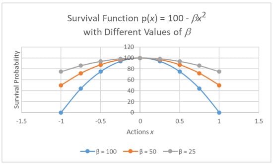
Figure 1.
The survival function.
To perform analysis on the model in (2), the actions of the individuals should be thought of as random variables, each of which can be any real number. Furthermore, as a first approximation, consider the case where the individuals choose their actions—and those which they, as leaders, believe are best for survival—independently and randomly from an arbitrary probability distribution with mean and standard deviation . This is surely not what happened in early human groups, although this may be what happened in early groups of cellular organisms. Nevertheless, analysis in this case will still provide some interesting insights. The consequences of relaxing this assumption are examined in Section 5.
In the context of this setting, the value of can be interpreted as the degree to which the individuals tend to choose actions on their own that are aligned with the well-being of the community: the closer is to 0—the actions that maximize —the more the individuals tend to choose actions that result in a high probability of group survival. The value of reflects the degree to which individuals choose actions that are different from the mean: the larger the value of , the more individual actions vary from the mean and hence the more diversity there is in their choice of actions.
3. Analytical Results for Large Groups
The next step to answering the questions posed in Section 2 is to use the actions represented by the random variables to compute, from (2), the following random variable that represents the likelihood of survival:
Even without knowing the distribution function of , it follows that
From (4), one sees that, for a fixed value of , the expected probability of survival becomes smaller as the group size increases. This observation is consistent with some prior research in which increased team size leads to reduced communication between group members and therefore reduces overall performance (see [15] and also [16]). Other literature points to larger groups having better performance, for example, due to more diversity. From a leadership point of view, it might actually be the case that increasing group size, up to a point, is better but that eventually the group is too large for a single leader to manage optimally. In any event, this model shows that large groups whose individuals randomly choose their actions independently—that is, large groups with no leadership—have little chance of survival. This also means that, as the group size increases, so does the need for leadership so as to improve the chances of survival.
To answer the questions posed in Section 2, it is necessary to know the probability distribution of , which is not readily available. However, it is possible to rewrite as follows:
In this form, when n is large, the central limit theorem allows the use of a normal distribution as an approximation to the distribution function of because is the average of the iid random variables . Specifically, if and , then is approximately normal, with a mean of and a standard deviation of . Then, , being a linear transformation of , also follows a normal distribution, specifically:
It is now possible to use (5), with the corresponding cumulative distribution function and density function , to answer the questions posed in Section 2. This is done first for groups that, without leadership, have a positive probability of survival. The corresponding questions for groups that have no chance of surviving without a leader are addressed subsequently in Section 3.2. To this end, let be the actions chosen by the n individuals in a group without a leader with the survival function given in (3). Proofs for all results are provided in Appendix A.
3.1. Analysis for Leaderless Groups with Positive Survival Probability
Throughout this section, it is assumed that the group has a positive probability of survival without a leader—that is, , where x are the actions that the individuals take without a leader. The first quantity of interest is the fraction of individuals whose leadership would result in an increased likelihood of survival. This fraction is the same as the probability that a leader chosen at random from the group improves the probability of survival. Thus, suppose that this random leader induces the individuals to take actions , which are also iid random variables following the same distribution as the actions x. The desired fraction is then
In the foregoing case, it is also interesting to know the chances of survival with such a leader, on average. This value is given by
The next quantity of interest is the fraction of leaders who would reduce the chances of survival, but still have some positive probability of survival—that is,
In the foregoing case, the expected (positive) survival probability when the leader decreases the chances of survival is given by
The final quantity of interest for a leaderless group that has a positive probability of survival is the fraction of individuals who, as leaders, would reduce the chances of survival to 0—that is,
3.2. Analysis for Leaderless Groups with No Chance of Survival
Throughout this section, it is assumed that the group has no chance of survival without a leader—that is, . The first quantity of interest is the fraction of individuals whose leadership would result in a positive probability of survival. This fraction is the same as the probability that a leader chosen at random from the group improves the probability of survival to a positive value. Thus, suppose that this random leader induces the individuals to take actions . The desired fraction is then
In the foregoing case, it is also interesting to know what the group’s survival probability is with such a leader, on average. This value is given by
The final quantity of interest is the fraction of leaders under whom the group has no chance of survival—that is,
The final question posed in Section 2 is about the importance of choosing a good leader. To this end, it would be desirable to know the expected probability of survival under the best leader, under the second-best leader, and so on. However, these results are challenging to compute analytically and so are estimated using simulation. This, together with estimates of the probabilities in Equations (6)–(13) for small groups, is reported in the next section.
4. Simulation Results for Small Groups
The results obtained in Section 3 are approximations that pertain to large groups. In this section, simulations are used to see how accurate the approximations are for small groups.
To implement the simulation, it is necessary to choose a specific distribution for the actions of the individuals. As a starting point, suppose that, in the absence of a leader, these actions follow a uniform distribution with mean 0, indicating that individuals on average choose actions that are good for survival. While, in theory, an individual’s action can be any real number, from a practical perspective, their actions are restricted to the interval , where a is a controllable measure of the diversity (variance) of the individuals’ actions without a leader. In summary, the actions are iid random variables with .
With this assumption, it is possible to compare the theoretical results in Section 3 pertaining to large groups with the simulation results described in this section for small groups. To this end, because each , it follows that and . Thus, for large n, from (5),
While there are several research studies that have looked at the effect of heterogeneity or diversity in teams, there seem to be fewer studies that actually look at the impact of diversity on a leader’s actions. Previous research has shown that while some diversity can be positive, in that it brings different external perspectives to the performance of a team, diversity will also have negative effects. In [17] it is shown that functional and tenure diversity are negatively correlated to team performance. A higher level of diversity of actions in such a situation means that achieving coordination of those diverse actions is also important. Prior research shows that increased diversity within a team also introduces other factors that may affect the functioning of the team. One of the immediate consequences of diversity is conflict, which in turn affects team performance (see [18] and also [19]). Thus, higher diversity of actions within teams necessitates a focal person—that is, a leader—to coordinate actions so that the team is effective (see [20]).
4.1. General Comments about the Simulations
Simulation results are collected for various combinations of the size of the groups (n), the harshness of the environment (), and the diversity of the individuals’ actions (a). In so doing, it is important to note that for fixed values of n and , the value of a must be chosen carefully for the effect of a to be interesting. This is because the effects of n and result in different ranges of a over which statistics of interest vary enough so that the effect of a can be easily observed. For example, when and , for any value of a above 8, almost every leader will result in the group having no chance of survival, making it difficult to observe the effect of changing a across values greater than 8 on the fraction of leaders who result in no chance of survival.
In general, two extreme scenarios are possible. One is when the environment is so unfavorable that the group will not survive, no matter which leader, if any, is chosen. This scenario corresponds to all groups having a 0% chance of survival without a leader and each leader providing a 0% chance of survival. Another such scenario is when the environment is so favorable that the group will survive, no matter which leader, if any, is chosen. This scenario corresponds to all groups having a 100% chance of surviving without a leader and each leader providing a 100% chance of survival. In both of these extreme cases, leadership has no impact on the survival of the group and so one would not expect leadership to emerge. Hence, we choose parameter values to explore the range of scenarios between these two extremes to demonstrate when leadership can have an impact on survival and will be likely to emerge.
To determine the values of n, , and a used in the simulations, we focused on small values of n, as this is the purpose of the simulation experiments. This being the case, we chose n = 5, 10, and 20. Here, n = 5 represents the smallest sort of group that is likely to require the coordination of a leader and n = 20 represents the largest group for which the simulation results may vary significantly from the analytical results. As the effects of and a are dependent on each other, after selecting n, we can then set either or a to arbitrary baseline values and vary the other parameter to obtain meaningful results. In this case, we chose to set = 1, 2, and 4. Finally, for fixed values of n and , values of a were chosen so that the following statistics could be computed using a reasonable number of “survival groups” (i.e., groups that have a positive probability of surviving without a leader):
- The fraction of leaders who are “beneficial leaders” (i.e., leaders who increase the survival probability of the group when compared to having no leader) and the corresponding average improvement in survival probability under such beneficial leaders.
- The fraction of leaders who are “harmful leaders” (i.e., leaders who decrease the survival probability of the group but still maintain a positive probability of survival) and the corresponding average decrease in survival probability under such harmful leaders.
- The fraction of leaders who are “deadly leaders” (i.e., leaders who result in the group dying off because the survival probability under their leadership is 0).
For “non-survival groups” (i.e., groups that would not survive without a leader), the fraction of leaders that are “survival leaders” (i.e., leaders that result in a positive probability of survival) and the average survival probability over all such leaders are calculated. Finally, over all groups, the average survival probability of the best leader, the second-best leader, and so on are also computed.
In performing these simulations, a sufficient number of groups are generated so that for each desired statistic, there are exactly 1000 cases of that type over which averages are computed. Thus, for example, for groups that have a positive probability of survival with no leader, when , , and , it was necessary to generate 580,974 groups to ensure that there were 1000 groups having at least one deadly leader.
4.2. Simulation Results on the Leaders
Figure 2, Figure 3, Figure 4 and Figure 5 contain results for beneficial leaders of survival groups, harmful leaders of survival groups, deadly leaders of survival groups, and survival leaders of non-survival groups, respectively. The x axis in these graphs represents the various values of n, , and a over which the simulations were performed, and the y axis represents the fraction of leaders with the corresponding survival property for the figure. Tick marks associated with each bar indicate the fractions obtained from the analytical formulas in Section 3 for the corresponding values of the parameters n, , and a associated with that bar. When interpreting the charts, it is important to observe that although the values are the same for each value of n, the a values are different with different values of n. Although this makes the effect of a on the various fractions obvious, determining the effect of n requires simultaneously considering the effect of a. This can be done by considering the different values of a that provide similar results for different values of n. The following are some key observations from Figure 2, Figure 3, Figure 4 and Figure 5:
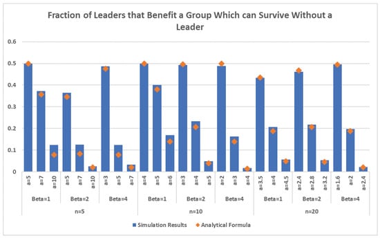
Figure 2.
Results for beneficial leaders of survival groups.
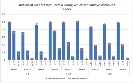
Figure 3.
Results for harmful leaders of survival groups.
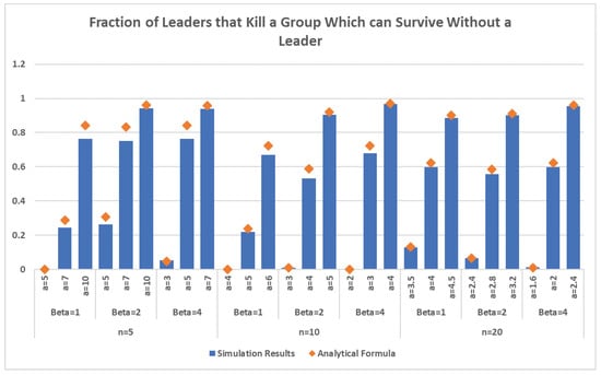
Figure 4.
Results for deadly leaders of survival groups.
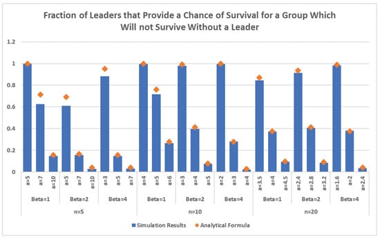
Figure 5.
Results for survival leaders of non-survival groups.
- For survival groups: Across all values of the parameters, the fraction of beneficial and harmful leaders is approximately the same—which agrees with the analytical results from (6) and (8) for large groups—as can be seen by observing that Figure 2 and Figure 3 are nearly identical. This is not surprising because when leaders randomly choose ideal actions for individuals that do not end up killing the group, one would expect an equal number of better and worse leaders. Moreover, as can be seen from Figure 4, for fixed values of n and , as the actions of the individuals become more variable—that is, as a increases—the fraction of deadly leaders increases. This same result holds for fixed values of n and a as the environment becomes more challenging—that is, as increases. This is because, in either case, the ideal actions chosen by leaders are more likely to result in the group dying off.
- For non-survival groups: As can be seen from Figure 5, for fixed values of n and , as the individuals become more diverse—that is, as a increases—the fraction of survival leaders decreases. This same result holds for fixed values of n and a as the environment becomes more challenging—that is, as increases. This is because, in either case, fewer leaders are able to identify actions that lead to group survival.
- For all groups The range of values of a over which groups have some chance of survival shrinks as n increases. This can be seen in Figure 4, which shows that when , groups of size have some non-deadly leaders in a range of to 10, while a corresponding range for groups of size when is to 4.5. Similarly, for non-survival groups, as seen in Figure 5, when , groups of size have some chance of survival in a range of to 10, while a corresponding range for groups of size when is to 4.5. Larger values of also have a shrinking effect on valid ranges of a for both survival and non-survival groups, but to a much lesser degree. This means that the larger the groups, and the harsher the environment, the more important it is to survival for individual actions to be coordinated, and hence the more important it should be to have a good leader, as confirmed by the foregoing results.
Taken together, the above-mentioned results provide evidence for the tradeoff between group size, harshness of the environment, and diversity of actions. Specifically, harsher environments, more diverse actions, and larger group size hinder group survival on average, and also point to the importance of having good leaders. These results contribute to previous findings that harsher environments facilitate the emergence of leaders (see [21]) and that increased heterogeneity—and thereby diversity—in teams could help or hinder performance in harsher environments depending on how well the group adapts (see [22]).
Moreover, in all of these cases, the analytical results associated with large groups derived in Section 2 are relatively close to the simulation results for small groups (see the tick marks in Figure 2, Figure 3, Figure 4 and Figure 5). In fact, the smaller the values of a and and the larger the value of n, the closer the analytical and simulation results are.
4.3. Simulation Results on the Survival Probabilities
The graphs in Figure 6, Figure 7 and Figure 8 are similar to those in Figure 2, Figure 3, Figure 4 and Figure 5 except that the y axis represents survival probabilities of interest. Figure 6 and Figure 7 correspond to survival groups and Figure 8 corresponds to non-survival groups. The vertical bars in Figure 6 show the average probability of survival for a survival group with a beneficial leader, and the tick marks in Figure 6 show the average probability of survival for a survival group without a leader. Similarly, Figure 7 depicts results for harmful leaders of survival groups. The vertical bars in Figure 8 show the average probability of survival for a non-survival group with a beneficial leader. Recall that, for a non-survival group, the probability of survival without a leader is 0 and so Figure 8 does not include tick marks. The following are key observations from these graphs:
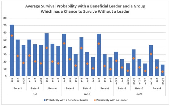
Figure 6.
Results for survival probabilities with a beneficial leader of a survival group.
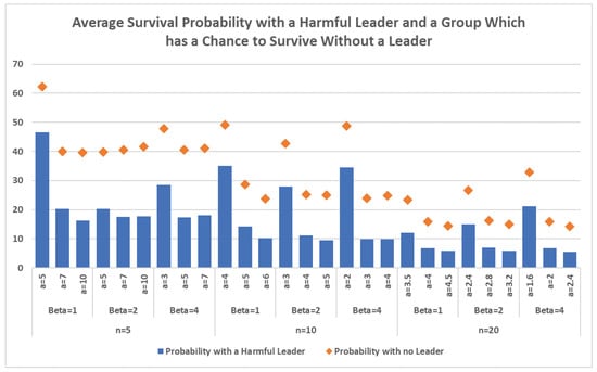
Figure 7.
Results for survival probabilities with a harmful leader of a survival group.
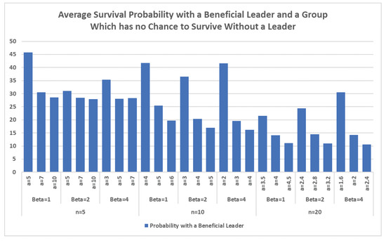
Figure 8.
Results for survival probabilities with a beneficial leader of a non-survival group.
- For groups that have a positive probability of survival with no leader: For fixed values of n and , as the individuals become more diverse—that is, as a increases—the average survival probability over all better leaders and all worse leaders decreases. Over better leaders, this decrease is more pronounced the larger the value of n. This means that the more diverse the individuals are in choosing their actions, the less a leader can improve the survival probability (or the more a leader can harm the survival probability). In contrast, for fixed values of n and a, the average survival probabilities over better and worse leaders remain relatively constant as the environment becomes more challenging—that is, as increases.
- For groups that would not survive without a leader: For fixed values of n and , as the individuals become more diverse—that is, as a increases—the average survival probability over all survival leaders decreases. The same is true for fixed values of n and a, as the environment becomes more challenging—that is, as increases—although less data points are available in this case as the range of values of a over which the simulations are performed changes as increases. This means that the more diverse the individuals are, or the more challenging the environment, the less effective survival leaders become.
In all of these cases, the analytical results associated with large groups are relatively close to the simulation results (except for and the large value of ). Furthermore, the smaller the values of a and and the larger the value of n, the closer are the analytical and simulation results.
4.4. Simulation Results on the Importance of Having a Good Leader
It has been shown that as certain conditions within groups change, the importance of leadership to a group’s survival increases. The next step to understanding the evolutionary significance of leader emergence is to ask the question: Does the quality of the leader matter and, if so, in what ways? Although leadership itself is important, it is also useful to understand the quality of the different potential leaders that would emerge in a group or a community. This is because individuals who successfully emerge as leaders may or may not be equally effective in carrying out their leadership duties (see [23]). Previous research indicates that certain kinds of leadership qualities or traits do make a difference in a leader’s effectiveness (see, for example [24]). However, from an evolutionary survival perspective, and in keeping with this paper’s purview, it is especially important to compare the effectiveness of all potential leaders and hence rank them from most effective to least effective. The most effective leader is defined in our model as one who achieves the best coordination and hence survival probability. The least effective leader is one who achieves the lowest survival probability. The results discussed below show that, in more diverse groups and harsher environments, the differences in survival rates between better and worse leaders are more pronounced and so the importance of selecting a better leader is more crucial.
Figure 9 shows the effects of the quality of the leader—that is, the best leader, the second-best leader, and so on—on the survival probability of the group for different levels of diversity. Specifically, the three curves in Figure 9 show the effect of the quality of the leader on the average survival probability for 1000 groups of size for and , and 6, respectively. The x axis represents the rank order of the leaders (1 is the best leader, 2 is the next best leader, and so on) and the y axis represents average survival probability. The dotted line in each curve is the average survival probability of the 1000 groups under no leader. As one would expect, for a fixed quality of leader, the average survival probability decreases as diversity increases—that is, as a increases. What is interesting, however, is that for , the survival probability decreases almost linearly in the quality of the leader. However, as a increases, the curves become increasingly more nonlinear, with a steeper drop-off in survival probability from the best leader to the second-best leader and to the third-best leader. Similar patterns hold for and 4 and over all values of n tested (however, the larger the value of n, the lower the curve). This means that, as diversity increases, having a good leader is ever more important to survival when the size of the group and the harshness of the environment are fixed.
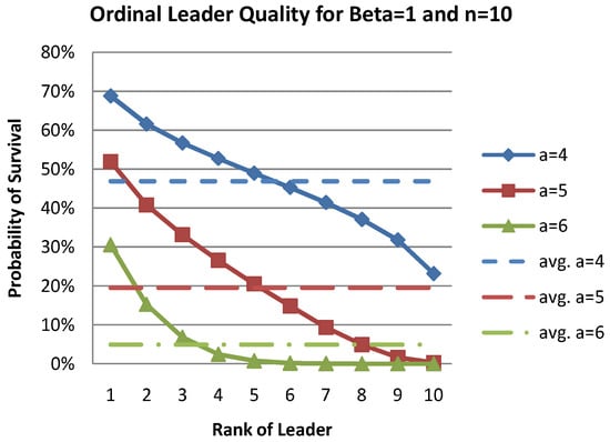
Figure 9.
Results for importance of having a good leader when = 1 and n = 10.
Figure 10 shows the effects of the quality of the leader on the survival probability of the group for different values of the harshness of the environment. Specifically, the three curves in Figure 10 show the effect of the quality of the leader on the average survival probability for 1000 groups of size for and , and 4, respectively. The x and y axes are the same as in Figure 9 and the dotted line in each curve is the average survival probability of the 1000 groups under no leader. The pattern seen in Figure 10 is similar to that seen in Figure 9 in that, as one would expect, for a fixed quality of leader, the average survival probability decreases as the environment becomes more harsh—that is, as increases. Furthermore, as increases, the curves become increasingly more nonlinear, with a steeper drop-off in survival probability from the best leader to the second-best leader and to the third-best leader. This means that, as the environment becomes more harsh, having a good leader is ever more important to survival when the size of the group and the variability in agent actions are fixed.
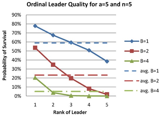
Figure 10.
Results for importance of having a good leader when a = 5 and n = 5.
In summary, it is most important to survival to identify a good leader when either there is a lot of diversity or the environment is harsh, all else being the same.
5. A Model with Dependent Actions
One of the key assumptions in the model in Section 2 is that the actions taken by the individuals are independent of each other. While this assumption leads to the ability to obtain analytical results, this may not always be the case. Even without the presence of a leader, individuals within a group may be motivated to work together or in unison due to several reasons. First, the nature of a task may encourage them to act in a similar and coordinated manner. This is sometimes called pooled interaction. Here, the effectiveness of the team depends on the amount of information and resources pooled or aggregated by the team members. Second, team members may be affectively or emotionally bound by their desire for belonging to a particular group (social or group identity). In both cases, the actions taken by group members are not independent of each other, but are guided by a common goal or the nature of the task. In this section, a new model is proposed in which it is possible to control the degree to which the actions of individuals depend on each other. Simulation results with the new model are also presented.
5.1. Model Development for Cohesiveness
In the proposed model, a controllable parameter, in the form of a real number c, is introduced to represent the “cohesiveness” of the group. At one extreme, when the value of c is 0, the group has no cohesiveness and so the actions of the individuals are independent of each other. At the other extreme, when , the group is completely cohesive and the actions of all individuals are identical. More generally, the closer the value of c is to 1, the closer the actions of the individuals are to each other.
To create such a model for a group of n individuals, n iid real numbers, , are generated from an arbitrary distribution. These values represent the actions that the individuals take when there is no cohesiveness (). At the other extreme, when there is full cohesiveness (), let the common action taken by all n individuals be the average of the foregoing actions—that is,
Then, for an arbitrary value of the cohesiveness parameter c with , each individual’s action is
Higher cohesion therefore results in more coordination and less conflict within the team and results in better team effectiveness. In an evolutionary sense, this means a higher chance of surviving. When the cohesion is high, the group members already have incentives (task type and desire to be part of the group) to take collective action. As explained previously, a leader’s role is to help facilitate coordination and ultimately to increase coordination within groups. Therefore, if the group members are already united and coordinated in their actions, the role of a leader will be less critical.
5.2. Results with Dependent Actions
As in the original model, it is now possible to compare the survival probability of the group when there is no leader, namely , to the survival probability, , when individual i becomes the leader and induces the individuals to perform actions , which the leader deems best for survival. The values for z are generated randomly and independently of the same distribution as the leaderless actions in (14). Simulation results obtained from this model are now reported.
To perform the simulations, as in the model in Section 2, individual actions that are independent come from . Statistics similar to those described in Section 4 are collected for all combinations of the size of the groups with and ; the cohesiveness of the group with ; the harshness of the environment with ; and the variability in the individuals’ actions with appropriate values chosen for a. Note that small values of n have been chosen as high levels of cohesiveness are intuitively unlikely in large groups. The results of the simulations appear in Figure 11, Figure 12 and Figure 13.
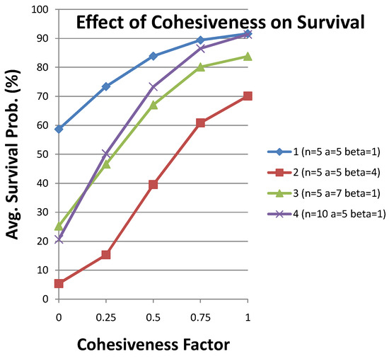
Figure 11.
The effect of cohesiveness on group survival without a leader.
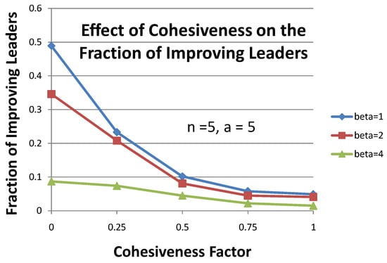
Figure 12.
The effect of cohesiveness on the fraction of improving leaders when a = 5 and n = 5.
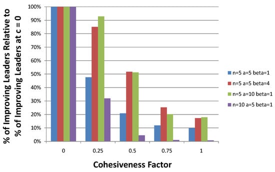
Figure 13.
The interaction between cohesiveness and n, a, and .
Figure 11 shows the fundamental effect of cohesiveness on the survival of the group when there is no leader. As one would expect, the more cohesive a group, the greater that group’s chances of survival without a leader. Further, the rate of increase in survival probability as a function of cohesiveness—indicated by the slopes of the line segments of the curves in Figure 11—is increasing with more diverse groups (compare curve 1 and curve 3), harsher environments (compare curve 1 and curve 2), and larger groups (compare curve 1 and curve 4). To see why cohesiveness improves group survivability without a leader, consider Equation (5): . From (5), it is seen that . Hence, as decreases, the expected survival probability without a leader increases. From (14), note that as cohesiveness c increases, decreases from to , resulting in a decrease in and a corresponding increase in the expected survival probability . That this relationship is magnified by a, n, and is again clear from (5).
Figure 12 shows how the increase in survival probability without a leader associated with increasing cohesiveness results in smaller fractions of leaders being able to improve group survivability. Though the figure shows results only for and , the same patterns were observed for other combinations of n and a. For a fixed group size (n) and level of diversity (a), the fraction of leaders that can improve group performance decreases as cohesiveness increases and the rate of this decrease is steeper for less harsh environments (smaller ). Furthermore, for a fixed level of cohesiveness (c), the harsher the environment (larger ), the smaller the fraction of leaders who will improve survival probabilities, with the difference between two such fractions for two different levels of harshness decreasing as cohesiveness increases (compare the curves for with and the curves for with , for example). The increase in survival probability associated with increasing cohesiveness seen in Figure 11 is the cause of the decrease in the fraction of leaders that can improve group survivability as cohesiveness increases and also explains the rate of this decrease being steeper for less harsh environments. The negative effect of harsher environments (larger ) on the fraction of leaders who will improve survival probabilities and the diminishing nature of this effect as c increases follow from the term in .
Figure 13 shows what happens to the fraction of leaders who improve group survivability that continue to improve group survivability as c increases. In the figure, columns in successive groups are all relative to the fraction of leaders who improve group survivability when . For example, suppose that for a fixed value of n, a, and , 50% of leaders improve the chance of survival when , 45% improve the chance of survival when , 40% improve the chance of survival when , 35% improve the chance of survival when , and 30% improve the chance of survival when . The corresponding columns in Figure 11 for , and 1 would be 0.50/0.50 = 100%, 0.45/0.50 = 90%, 0.40/0.50 = 80%, 0.35/0.50 = 70%, and 0.30/0.50 = 60%, respectively. The columns in Figure 11 corresponding to , and show that, for larger groups with less diversity in more benign environments, increasing cohesiveness rapidly eliminates members from the pool of leaders who improve survivability—in other words, in such an environment, increasing cohesiveness quickly results in few leaders who can provide survival benefits. The relationship with group size is consistent with previous results, but the other two relationships—diversity and harshness—are surprising given the previous results. The fact that cohesiveness more slowly eliminates improving leaders when diversity is high (see the columns for , and ) and environments are harsh (see the columns for , and ) may result from the fact that such leaders must already be extremely skilled to improve group survivability (see the discussion in Section 4.2).
In summary, while cohesiveness in general reduces the need for, and ability to find, improving leaders, there are still many situations—such as high levels of diversity and harsh environments—in which the evolutionary benefit of such leaders is evident.
6. Summary and Conclusions
In this work, models were created that provide a mathematical justification for the emergence and persistence of leadership. Specifically, using the theory of social coordination (see [25] and also [26]) as a foundation, it is shown that with a large number of groups, there are some leaders who are able to alter the behaviors of individuals to increase the group’s survival probability. Such leaders, therefore, provide an evolutionary benefit to these groups: groups with effective leaders are more likely to survive and persist. However, depending on the circumstances of the group, the probability of leadership improving the group’s chances of survival could be high or low. Several findings here help to explain these circumstances better. First, it is seen that diversity in actions or behaviors can hinder leadership in general, especially in large groups or harsh environments. These two conditions (diversity of actions and harshness of the environment) do not exclude the possibility that leaders will emerge—alternatively, it shows that leaders who emerge in conducive contexts (e.g., followers desperately looking for an idealistic leader) characterized by a smaller number of followers and a less harsh environment will have a better chance to lead the group to survival than a leader that emerges in a larger group under uncertain and harsh conditions.
Additionally, when looking at groups or teams with no leaders but which can survive (e.g., self-managing teams), we have shown that better leaders are more severely affected by the diversity of the actions of their followers than are worse leaders. We also found that for teams that absolutely need a leader for survival, both harsher environments and greater diversity of actions lead to lower survivability.
Other interesting results pertain to the quality of the leader. We ranked leaders from best (1) to worst (10). Our findings show that as group size increases, the effectiveness of the best to the second-best leader becomes more prominent (the relationship becomes nonlinear or drops off faster). A similar effect is also seen in increasingly harsh environments. These findings show that for larger groups in harsher environments, leader quality is much more important than in smaller groups. Additionally, the emergence process itself could be smoother and fairer for larger groups in harsher environments. Because, in larger groups, there is a greater difference between the effectiveness of the best and the second-best leader, the followers are more likely to choose the more effective leader and by a larger margin. This could perhaps explain the finding that the world’s most revered and admired leaders—such as Nelson Mandela, Mahatma Gandhi, and Martin Luther King Jr.—often arise in large communities under troubled and tested times.
To examine the impact of group cohesion on leader effectiveness, simulations were performed by relaxing the assumption that the actions of individuals are independent of each other. More action dependence means that team members are closer and more cohesive, resulting in a lesser need for leaders to engage in social coordination. Our results show that the effect of cohesiveness is more pronounced in harsher environments. Therefore, the presence of a leader is most important when environmental conditions are worse and there is little dependence between the follower actions. However, we also found that harsher environments and greater diversity result in a slower elimination of effective leaders as cohesiveness increases. One possible explanation could be that in harsher environments and when greater diversity is present, the roles of leaders could have been already less significant when cohesiveness is extremely low. Therefore, the slower loss of successful leaders with increasing cohesiveness could simply reflect the lower starting point.
Our models show the importance of contingencies involved in the outcomes relating to the existence of leadership. Taken together, our findings have important implications within a social as well as organizational context. While there have been several theories of leadership development and effectiveness (see [27]), our study and its findings provide key insights into the potential mechanisms of early group survival based on better and more effective processes of coordination. Additionally, the finding that the leader’s role is substantially more critical when the situations are less favorable (less task interdependence, harsher environments) confirms earlier findings of contingency theories of leadership, such as Fiedler’s findings on situational favorability and leadership effectiveness (see [28]). Our findings on leader ability and quality underlines previous findings on the use of specific styles or behaviors according to the specific contexts (e.g., situational models of leadership [29]). Teams or groups in the general society can be made up of people who may or may not take up the role of a leader. Understanding the appropriate conditions conducive (or not) to leadership is important in both managerial and general contexts. The knowledge that certain conditions can facilitate the emergence of a good leader can be important to leaderless groups in deciding whether to select a leader. Over the years, several groups of people have spontaneously formed movements and have had challenges related to unique but related criteria, such as the emergence and effectiveness of leadership both in larger and smaller communities (see [2]). Understanding the importance of the external environment (e.g., less harsh environment) as well as the internal environment (e.g., task interdependence) will go a long way in determining and perpetuating effective leadership in the larger society. This will also facilitate the survival of groups with leaders as opposed to leaderless groups.
Results from the models presented here are based on several assumptions. For example, we assume that, with regard to the emergence of leadership, selection occurs at the group level rather than at the individual level, which is not standard and may affect the plausibility of the model. However, this assumption is based on previous research that demonstrates the creation and evolution of more complex units (single-cellular to multicellular; individual to groups, etc.) such as that suggested by [4]. Our hypotheses and the related conceptual foundations and discussions highlight the role of leaders in facilitating processes such as coordination, communication, and complex learning that are outlined in [5].
Another limitation is that the survival function used here is concave and means that the survival probability monotonically decreases as the individuals’ actions are farther away from the actions that maximize the chances of survival. Moreover, in the simulations, it is assumed that each individual’s action is a random variable that follows a uniform distribution with a mean of 0 (so, on average, individual actions are aligned with the survival interests of the group). It might be interesting to see how the results obtained here change if the foregoing assumptions are relaxed. In addition, in the current “static” model, the actions of the individuals are interpreted as long-term behavior that affects the group’s long-term survival probability. Another direction for future research might be to develop a dynamic model in which the individual actions vary from one time period to another under the influence of a leader.
Another related area of interest is the effect of the visionary skill of the leader—as measured by how close the leader’s vision of ideal actions of the individuals is to those actions that maximize the group’s survival probability—and the charismatic skill of the leader to induce individuals to take the ideal actions envisioned by the leader. It might be possible to build mathematical models to study these leadership skills.
Author Contributions
Methodology, D.S. and J.S.; Project administration, J.S.; Software, D.S. and J.S.; Supervision, D.S.; Validation, S.K.; Writing—review and editing, S.K. All authors have read and agreed to the published version of the manuscript.
Funding
This research received no external funding.
Institutional Review Board Statement
Not applicable.
Informed Consent Statement
Not applicable.
Data Availability Statement
All data were generated randomly, as described in the paper.
Acknowledgments
We are grateful to two anonymous referees who understood the value of our contributions and whose comments were aimed at improving the exposition. We hope that we have achieved their goals.
Conflicts of Interest
The authors declare no conflict of interest.
Appendix A. Proofs of Analytical Results
Appendix A.1. Derivation of (6), (8), (10), (11), and (13)
Equations (6), (8), (10), (11), and (13) follow primarily from the independence of and , as follows:
Note that the last equation in (A1) is precisely (6).
Note that the last equation in (A2) is precisely (8). Also, in the following, note that (A3) below is (10), (A4) below is (11), and (A5) below is (13).
Appendix A.2. Derivation of (12)
Appendix A.3. Derivation of (7) and (9)
Now, (7) is derived as follows:
Consider the second term of the last expression in (A8) first. Noting that is the density of a truncated normal distribution, (A6) is used to obtain
Now, the integral in the first term of last expression in (A8) is evaluated by substituting to obtain:
The challenge in evaluating (A10) further is in evaluating and . To that end, the normal error function and are used. Recalling we calculate as:
Similarly, can be evaluated as follows:
Next, substituting (A11) and (A12) into (A10) gives
References
- Pietraszewski, T. The evolution of leadership: Leadership and followership as a solution to the problem of creating and executing successful coordination and cooperation enterprises. Leadersh. Q. 2019, 32, 101299. [Google Scholar] [CrossRef]
- Von Rueden, C.; Van Vugt, M. Leadership in small-scale societies: Some implications for theory, research, and practice. Leadersh. Q. 2015, 26, 978–990. [Google Scholar] [CrossRef]
- Van Vugt, M.; Grabo, A.E. The Many Faces of Leadership: An Evolutionary-Psychology Approach. Curr. Dir. Psychol. Sci. 2016, 24, 484–489. [Google Scholar] [CrossRef]
- Szathmary, E.; Smith, J.M. The major evolutionary transitions. Nature 1995, 374, 227–232. [Google Scholar] [CrossRef] [PubMed]
- Richerson, P.; Baldini, R.; Bell, A.V.; Demps, K.; Frost, K.; Hillis, V.; Mathew, S.; Newton, E.K.; Naar, N.; Newson, L.; et al. Cultural group selection plays an essential role in explaining human cooperation: A sketch of the evidence. Behav. Brain Sci. 2016, 39, e30. [Google Scholar] [CrossRef] [PubMed] [Green Version]
- Shang, Y. A note on the H index in random networks. J. Math. Sociol. 2018, 42, 77–82. [Google Scholar] [CrossRef]
- King, A.J.; Johnson, D.D.; Van Vugt, M. The origins and evolution of leadership. Curr. Biol. 2009, 19, R911–R916. [Google Scholar] [CrossRef] [Green Version]
- Forno, A.D.; Merlone, U. The Emergence of Effective Leaders: An Experimental and Computational Approach. Emergence Complex. Organ. 2006, 8, 36–51. [Google Scholar]
- Hannan, M.T.; Freeman, J. The population ecology of organizations. Am. J. Sociol. 1977, 82, 929–964. [Google Scholar] [CrossRef]
- Solow, D.; Szmerekovsky, J. Factors that Affect the Optimal Amount of Central Control in Complex Systems. Nav. Res. Logist. 2008, 55, 478–491. [Google Scholar] [CrossRef]
- Bass, B.M. From transactional to transformational leadership: Learning to share the vision. Organ. Dyn. 1990, 18, 9–31. [Google Scholar] [CrossRef] [Green Version]
- Halevy, N.; Berson, Y.; Galinsky, A.D. The mainstream is not electable: When vision triumphs over representativeness in leader emergence and effectiveness. Personal. Soc. Psychol. Bull. 2011, 37, 893–904. [Google Scholar] [CrossRef]
- Judge, T.A.; Colbert, A.E.; Ilies, R. Intelligence and Leadership: A Quantitative Review and Test of Theoretical Propositions. J. Appl. Psychol. 2004, 89, 542–552. [Google Scholar] [CrossRef] [PubMed]
- Graeff, C.L. The situational leadership theory: A critical view. Acad. Manag. Rev. 1983, 8, 285–291. [Google Scholar] [CrossRef]
- Blau, P.M. A formal theory of differentiation in organizations. Am. Sociol. Rev. 1970, 35, 201–218. [Google Scholar] [CrossRef]
- Shaw, M.E.; Harkey, B. Some effects of congruency of member characteristics and group structure upon group behavior. J. Personal. Soc. Psychol. 1976, 34, 412–418. [Google Scholar] [CrossRef]
- Ancona, D.G.; Caldwell, D.F. Bridging the boundary: External activity and performance in organizational teams. Adm. Sci. Q. 1992, 37, 634–665. [Google Scholar] [CrossRef] [Green Version]
- Jehn, K.E.; Northcraft, G.B.; Neale, M.A. Why differences make a difference: A field study of diversity, conflict, and performance in work groups. Adm. Sci. Q. 1999, 44, 741–763. [Google Scholar] [CrossRef] [Green Version]
- Pelled, L.H.; Eisenhardt, K.M.; Xin, K.R. Exploring the black box: An analysis of work group diversity, conflict, and performance. Adm. Sci. Q. 1999, 44, 1–28. [Google Scholar] [CrossRef] [Green Version]
- Kearney, E.; Gebert, D. Managing diversity and enhancing team outcomes: The promise of transformational leadership. J. Appl. Psychol. 2009, 94, 77–89. [Google Scholar] [CrossRef]
- De Hoogh, A.H.B.; Den Hartog, D.N.; Koopman, P.L. Linking the Big Five-Factors of personality to charismatic and transactional leadership; perceived dynamic work environment as a moderator. J. Organ. Behav. 2005, 26, 839–865. [Google Scholar] [CrossRef]
- Murray, A.I. Top management group heterogeneity and firm performance. Strateg. Manag. J. 1989, 10, 125–141. [Google Scholar] [CrossRef]
- Taggar, S.; Hackett, R.; Saha, S. Leadership emergence in autonomous work teams: Antecedents and outcomes. Pers. Psychol. 1999, 52, 899–926. [Google Scholar] [CrossRef]
- Judge, T.A.; Bono, J.E.; Ilies, R.; Gerhardt, M.W. Personality and leadership: A qualitative and quantitative review. J. Appl. Psychol. 2002, 87, 765–780. [Google Scholar] [CrossRef] [PubMed]
- Van Vugt, M.; Hogan, R.; Kaiser, R.B. Leadership, followership, and evolution: Some lessons from the past. Am. Psychol. 2008, 63, 182–196. [Google Scholar] [CrossRef] [Green Version]
- Calvert, R. Leadership and its basis in problems of social coordination. Int. Political Sci. Rev. 1992, 13, 7–24. [Google Scholar] [CrossRef]
- Dinh, J.E.; Lord, R.G.; Gardner, W.L.; Meuser, J.D.; Liden, R.C.; Hu, J. Leadership theory and research in the new millennium: Current theoretical trends and changing perspectives. Leadersh. Q. 2014, 25, 36–62. [Google Scholar] [CrossRef] [Green Version]
- Miller, R.L.; Butler, J.; Cosentino, C.J. Followership effectiveness: An extension of Fiedler’s contingency model. Leadersh. Organ. Dev. J. 2004, 25, 362–368. [Google Scholar] [CrossRef]
- Thompson, G.; Glasø, L. Situational leadership theory: A test from three perspectives. Leadersh. Organ. Dev. J. 2015, 36, 527–544. [Google Scholar] [CrossRef]
- Barr, D.R.; Sherrill, E.T. Mean and Variance of Truncated Normal Distribution. Am. Stat. 1999, 53, 357–361. [Google Scholar]
Publisher’s Note: MDPI stays neutral with regard to jurisdictional claims in published maps and institutional affiliations. |
© 2021 by the authors. Licensee MDPI, Basel, Switzerland. This article is an open access article distributed under the terms and conditions of the Creative Commons Attribution (CC BY) license (https://creativecommons.org/licenses/by/4.0/).