
Acceleration and Parallelization of a Linear Equation Solver for Crack Growth Simulation Based on the Phase Field Model


Abstract
:1. Introduction
2. Crack Growth Simulation Based on the Phase Field Model
2.1. The Two-Dimensional Case
- The direction of crack growth is automatically determined by the PDEs. Hence, total energy evaluation under multiple possible scenarios, which is needed in simulation methods based directly on (3), is not necessary;
- By introducing the phase field variable and the regularization parameter , the divergence of the stress at the tip of the crack is kept to a level manageable by numerical methods;
- It is not necessary to regenerate the mesh at every time step to conform to the crack boundary.
2.2. The Three-Dimensional Case
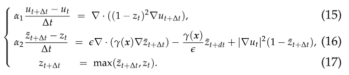
2.3. Temporal Discretization

3. Properties of the Coefficient Matrices Arising from Phase Field-Based Crack Growth Simulation
3.1. The Two-Dimensional Case
- The weak forms
- Properties of the coefficient matrix for
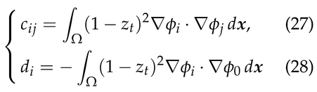
- Properties of the coefficient matrix for

3.2. The Three-Dimensional Case
- The weak forms
- Properties of the coefficient matrix for
- Properties of the coefficient matrix for
4. Application of the Incomplete Cholesky Preconditioner and Its Parallelization
4.1. The Incomplete Cholesky Preconditioner
| Algorithm 1: IC(0) decomposition |
| 1: for to n do 2: 3: for to n if do 4: 5: end for 6: end for |
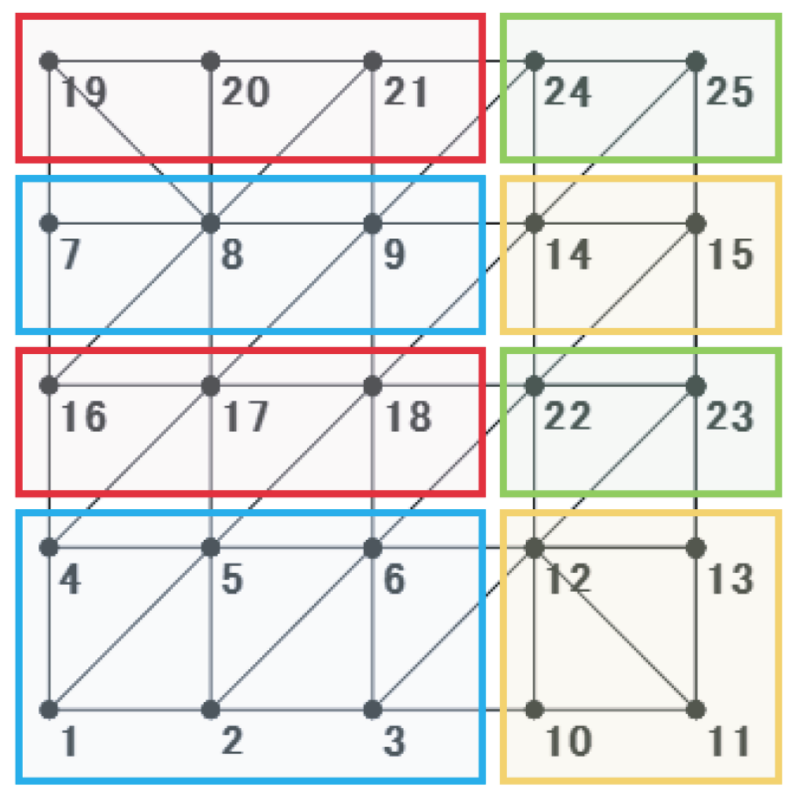
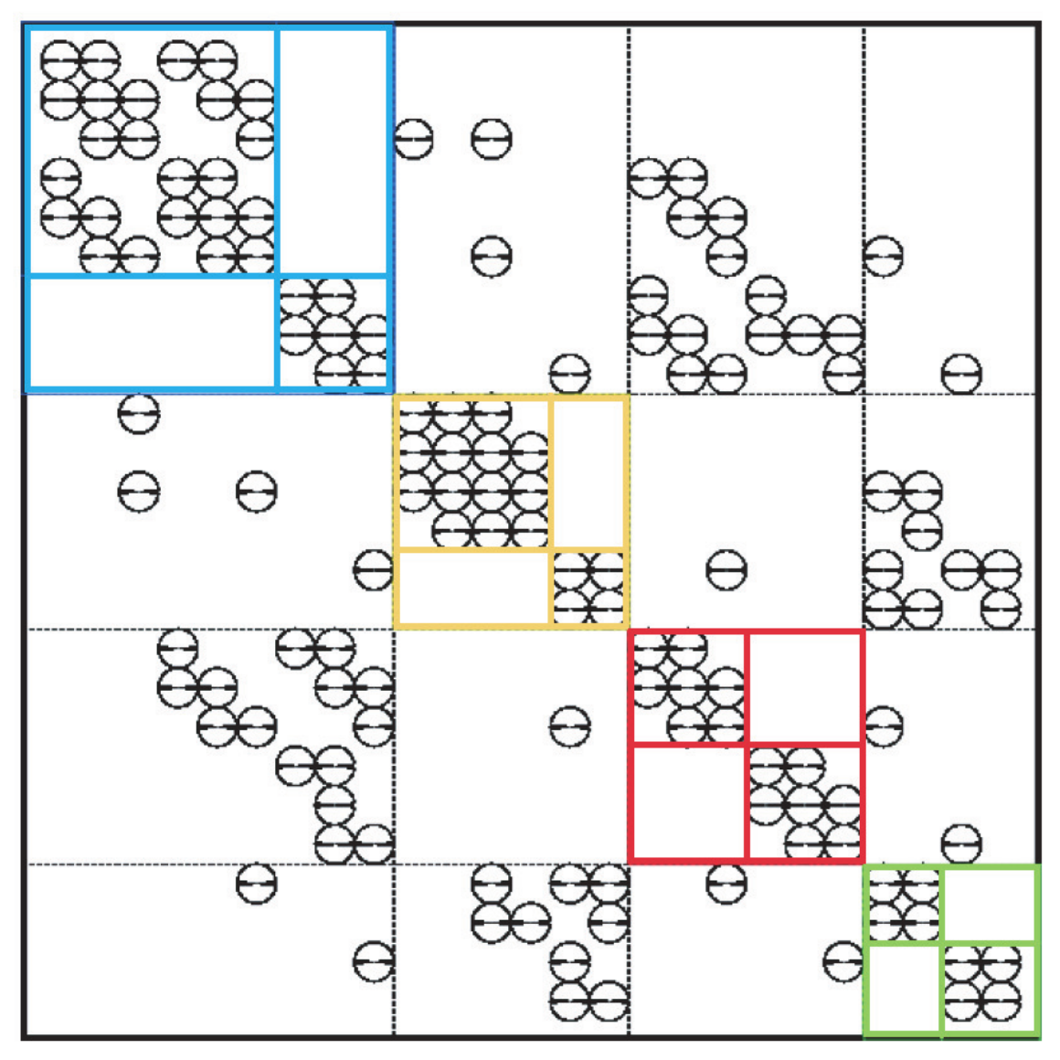
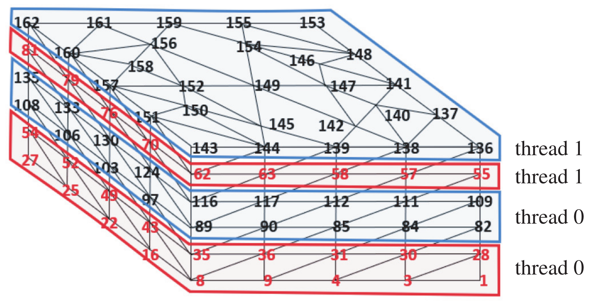
4.2. Parallelization by the Block Multi-Color Ordering
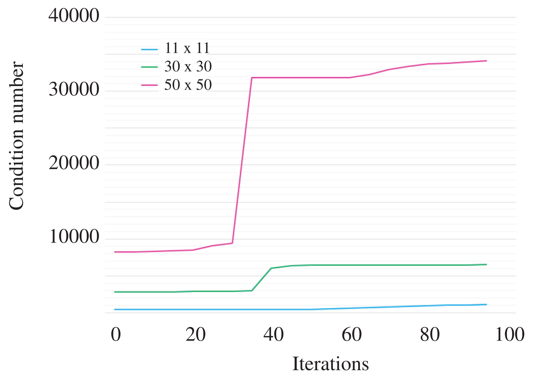
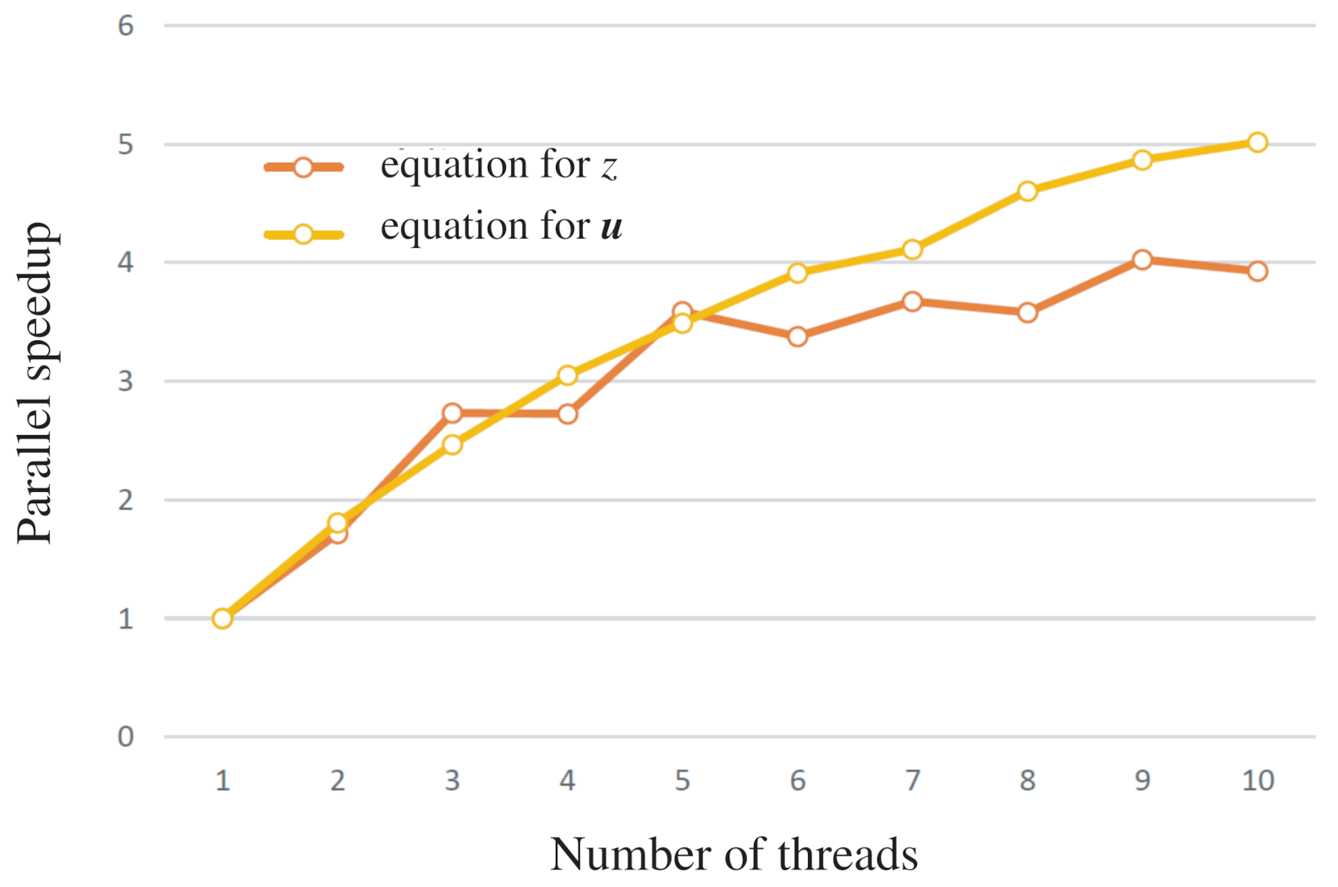
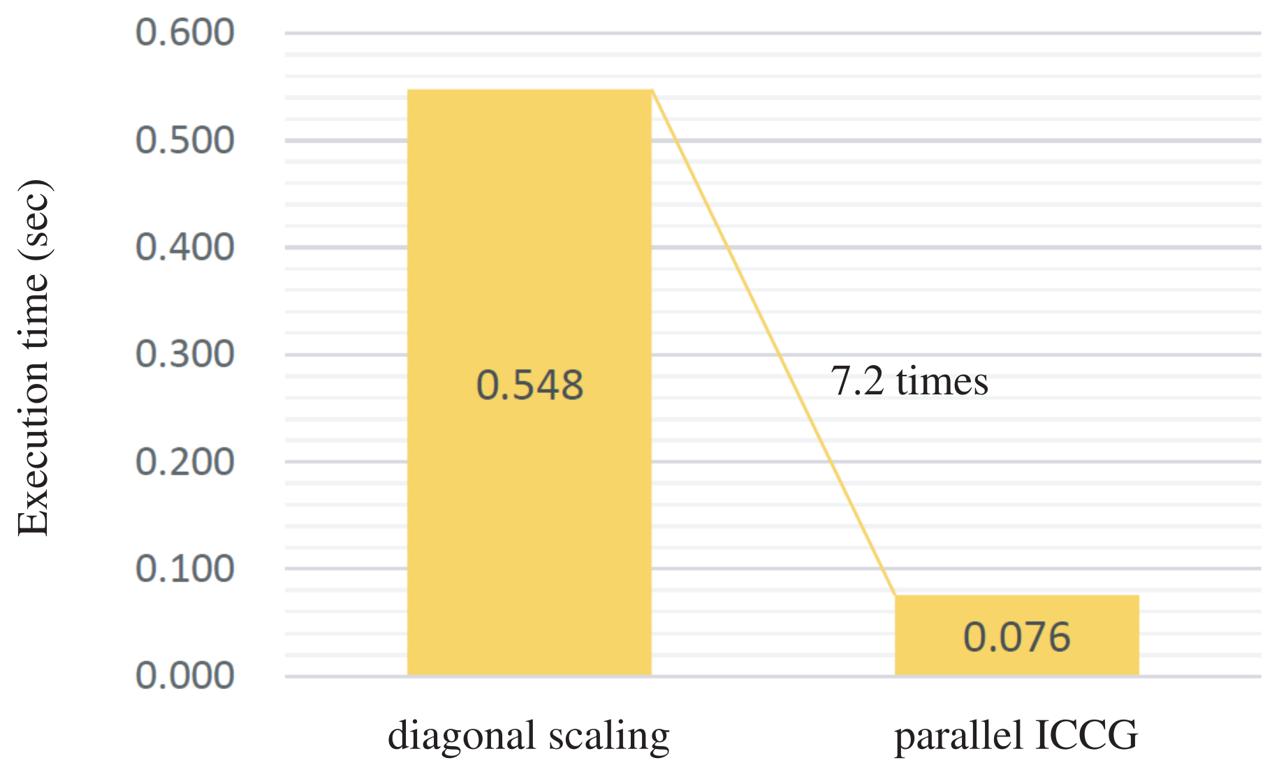
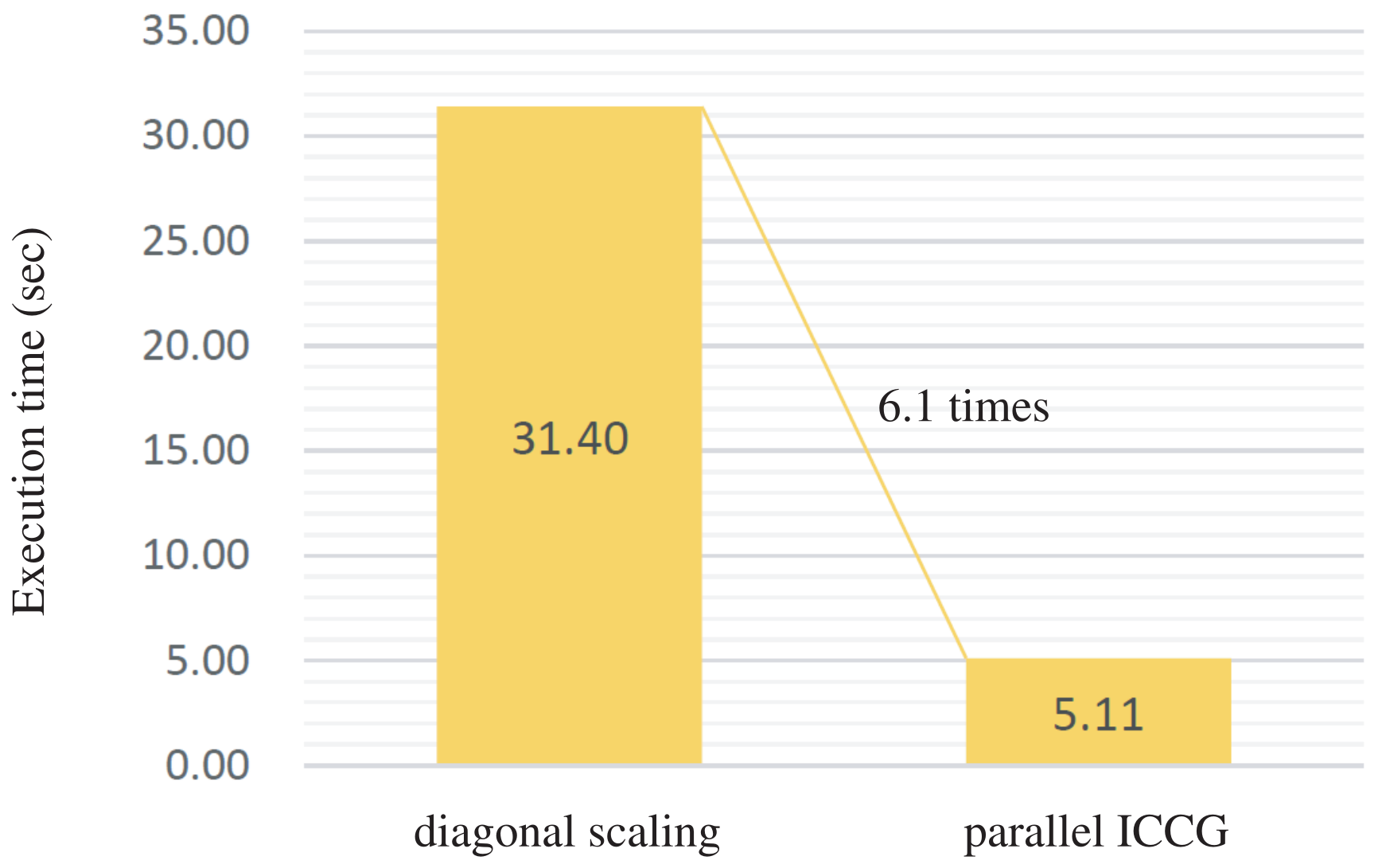
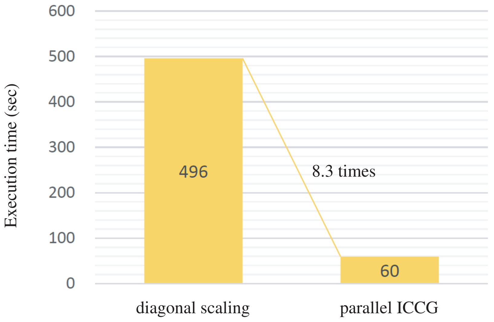
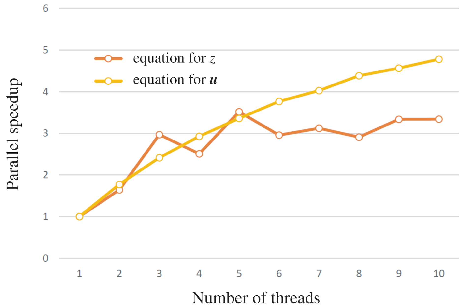
5. Numerical Results
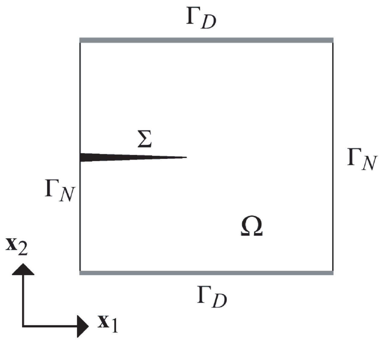
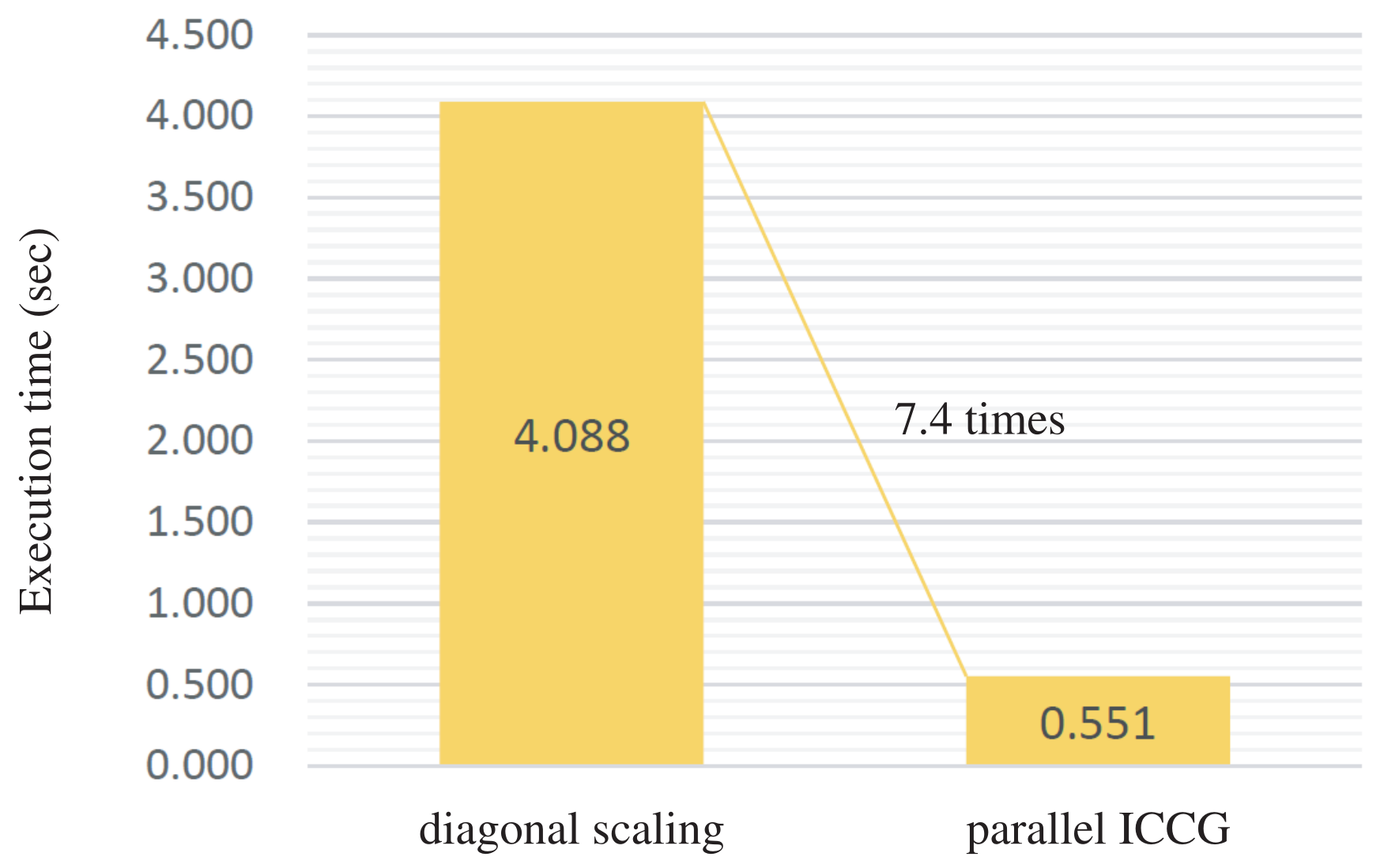
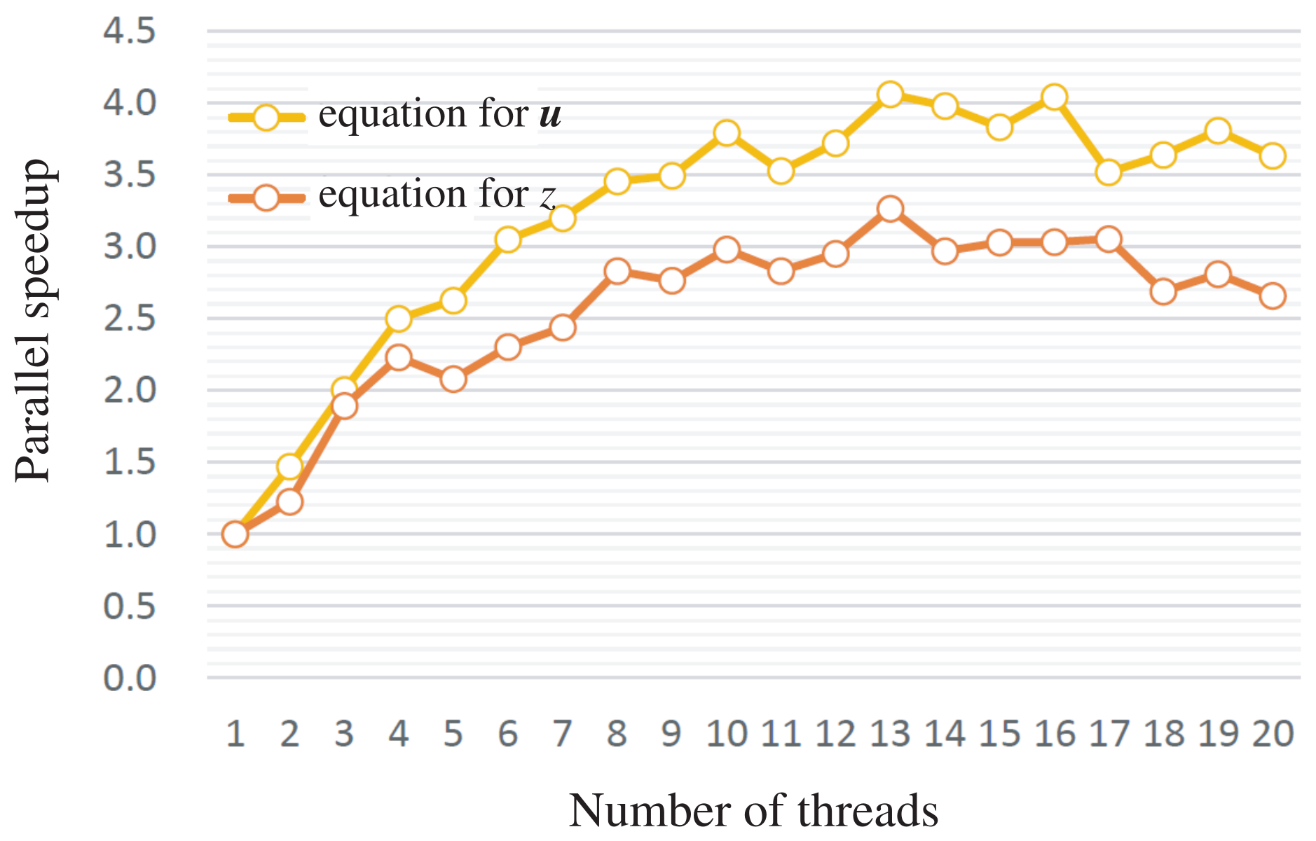
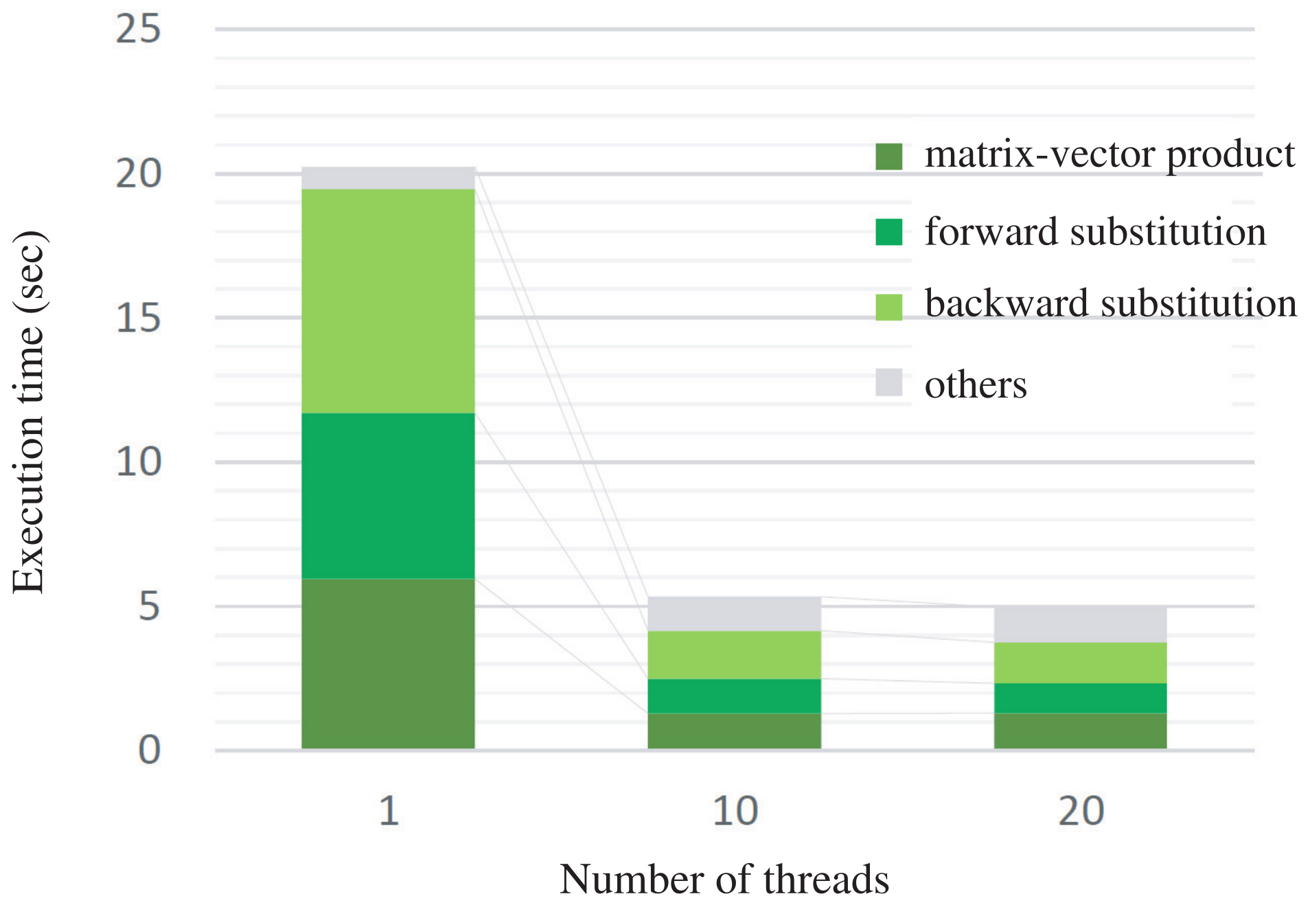
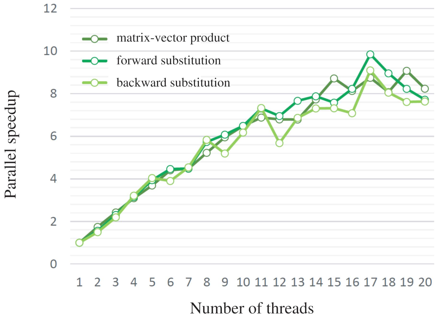
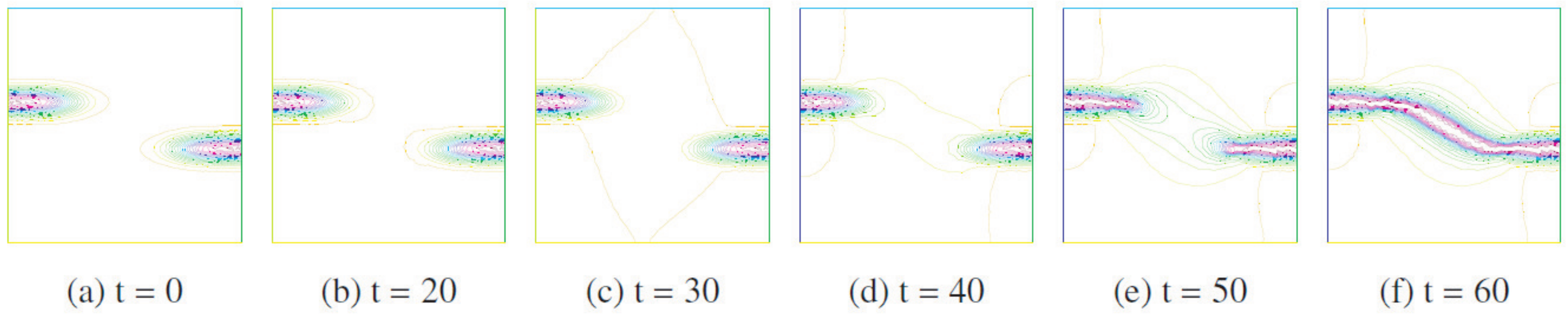
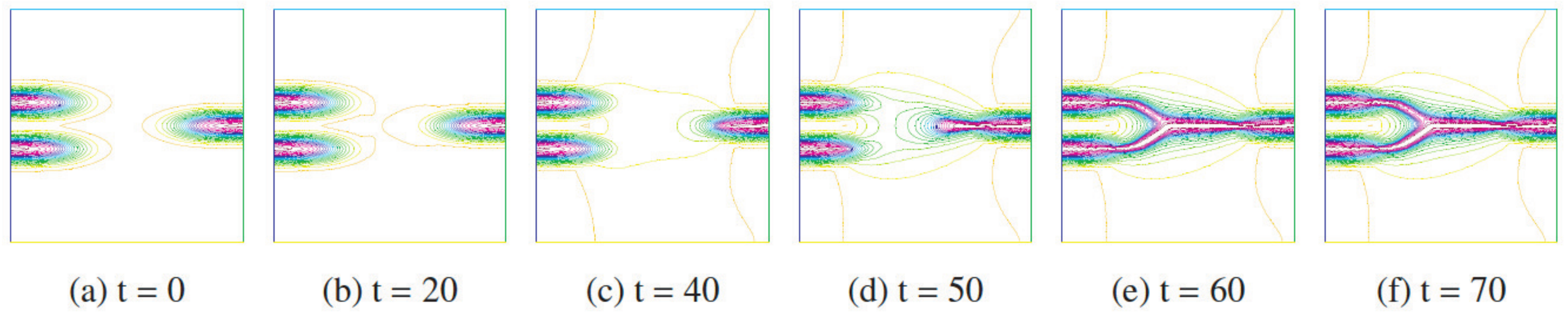
5.1. The Two-Dimensional Case
- Computational region: .
- Dirichlet boundary: .
- Neumann boundary: .
- Time step: .
- Parameters: .
- Initial conditions: , where .
- Convergence criterion of the CG method: relative residual .
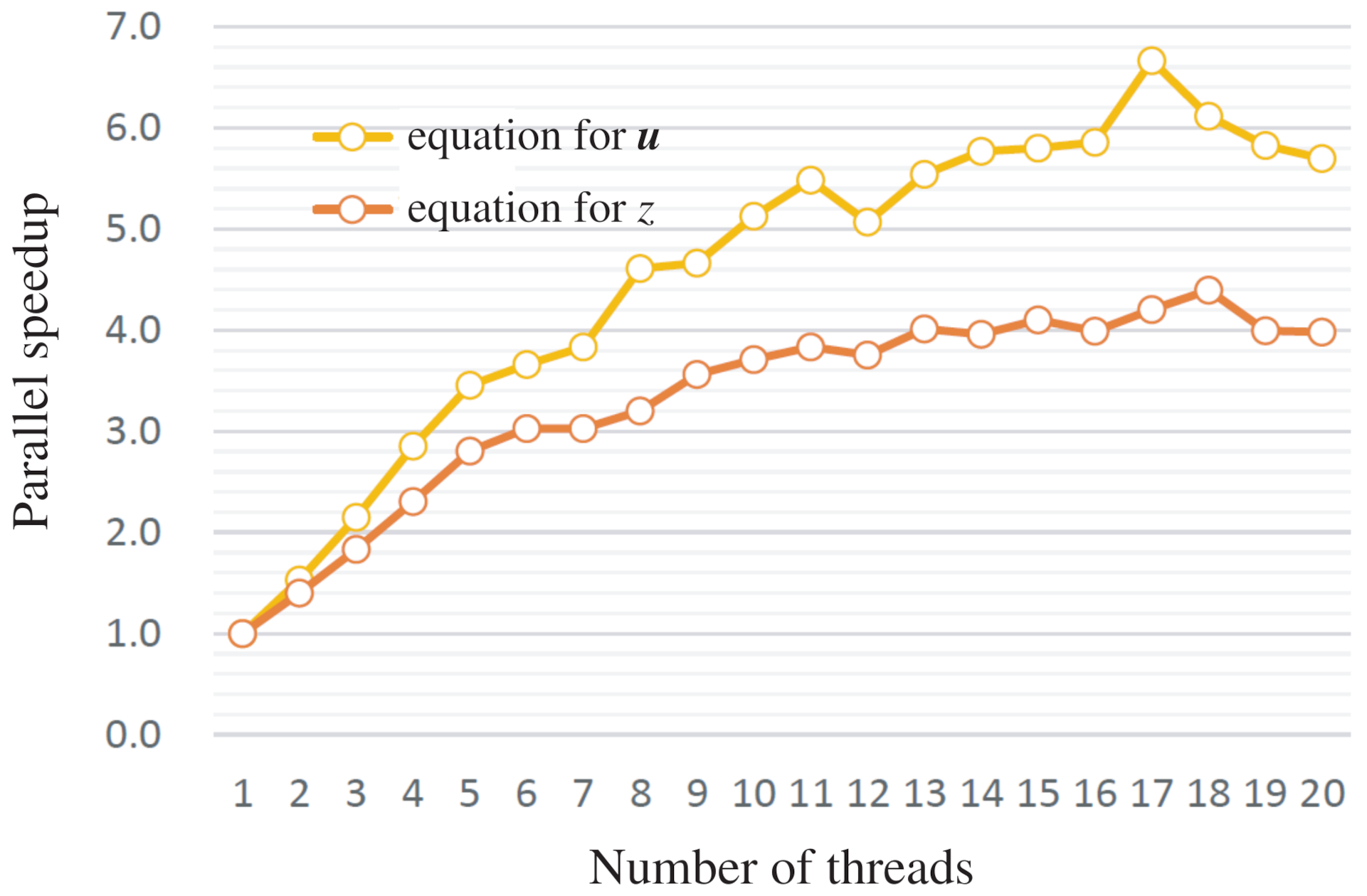
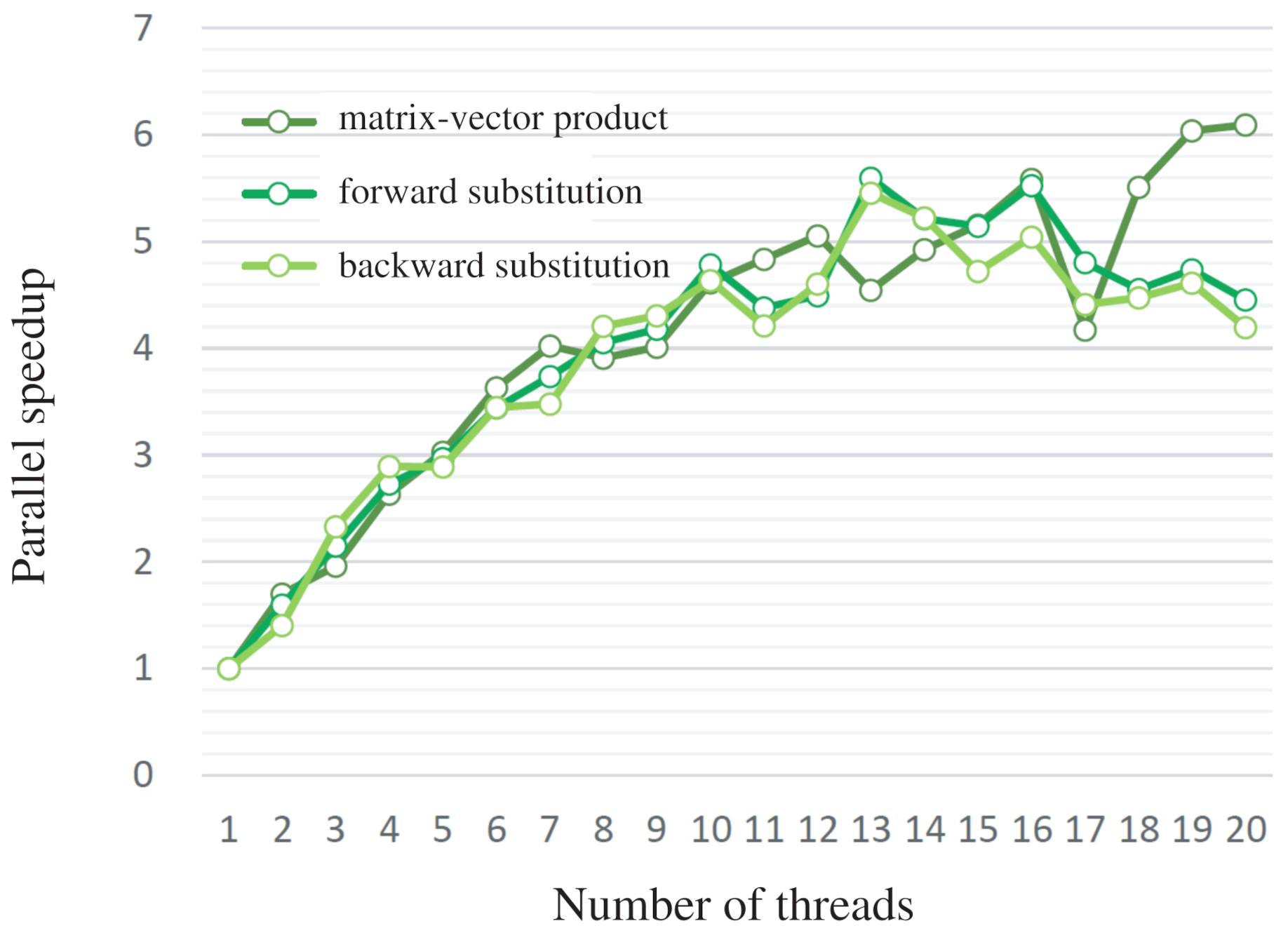
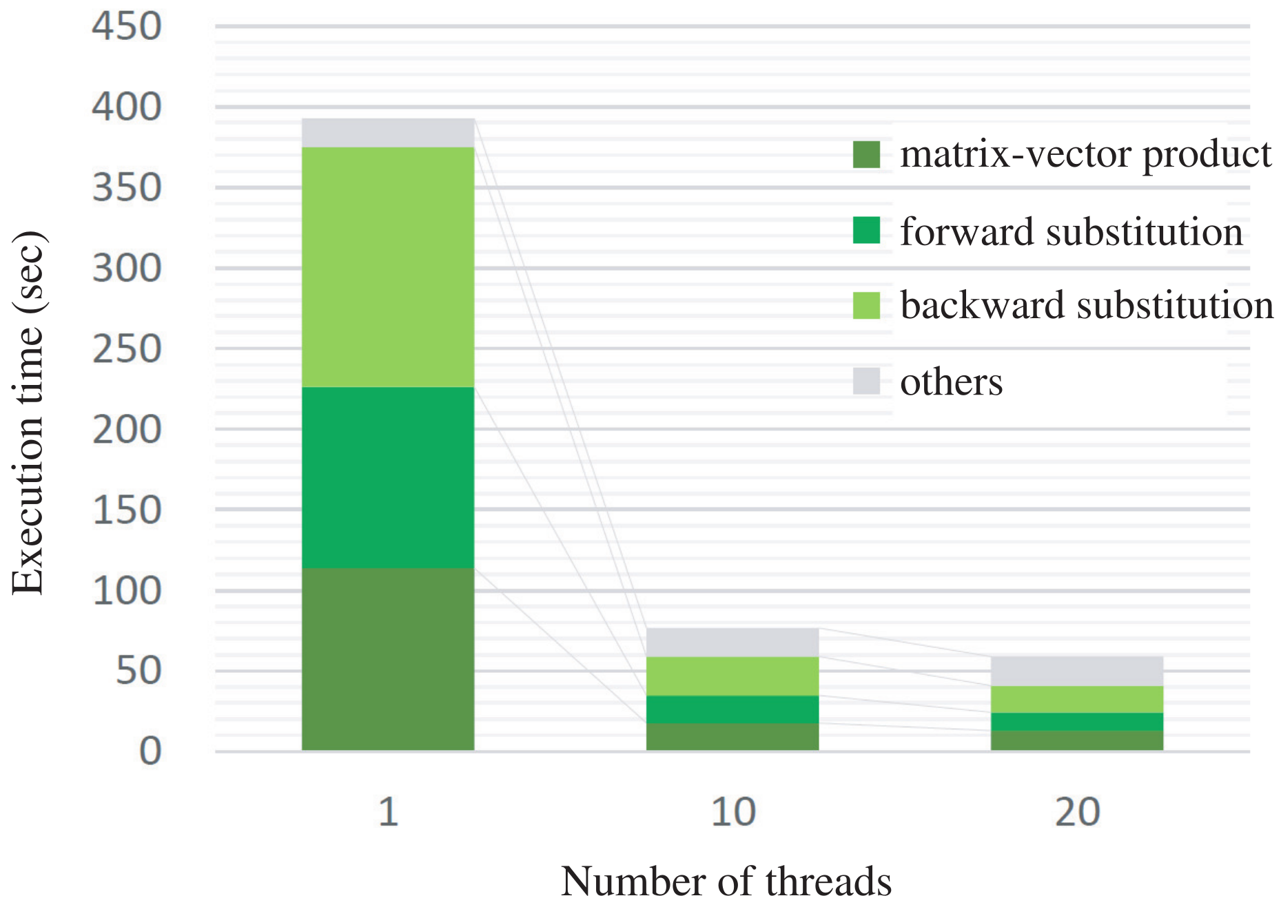
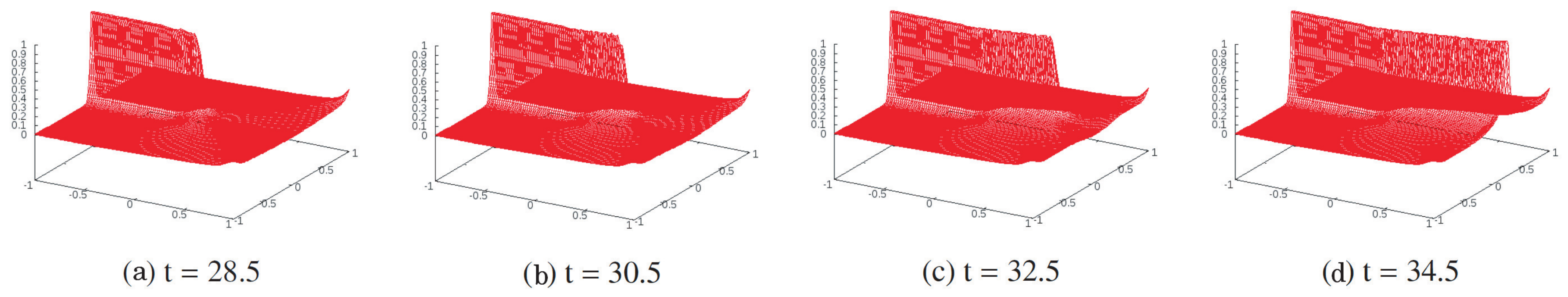
5.2. The Three-Dimensional Case
- Computational region: ;
- Dirichlet boundary: ;
- Dirichlet boundary: ;
- Neumann boundary: ;
- Time step: ;
- Parameters: ;
- Initial conditions: , where ;
- Convergence criterion of the CG method: relative residual .
6. Conclusions
Author Contributions
Funding
Institutional Review Board Statement
Informed Consent Statement
Data Availability Statement
Acknowledgments
Conflicts of Interest
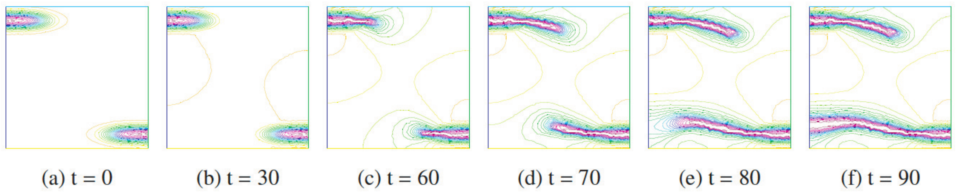
Appendix A. Two-Dimensional Crack Growth Simulation for Various Initial Conditions
- 1.
- 2.
- 3.


References
- Francfort, G.A.; Marigo, J.-J. Revisiting Brittle Fracture as an Energy Minimization Problem. J. Mech. Phys. Solids 1998, 46, 1319–1342. [Google Scholar] [CrossRef]
- Kimura, M.; Takaishi, T.; Alfat, S.; Nakano, T.; Tanaka, Y. Irreversible phase field models for crack growth in industrial applications: Thermal stress, viscoelasticity, hydrogen embrittlement. SN Appl. Sci. 2021, 3, 781. [Google Scholar]
- Takaishi, T.; Kimura, M. Phase field model for mode III crack growth. Kybernetika 2009, 45, 605–614. [Google Scholar]
- Takaishi, T. Numerical simulations of a phase field model for mode III crack growth. Trans. Jpn. Soc. Ind. Appl. Math. 2009, 19, 351–369. (In Japanese) [Google Scholar]
- Kobayashi, R. Modeling and numerical simulations of dendritic crystal growth. Phys. D 1998, 63, 410–423. [Google Scholar] [CrossRef]
- Provatas, N.; Elder, K. Phase-Field Methods in Materials Science and Engineering; Wiley-VCH: Weinheim, Germany, 2010. [Google Scholar]
- Iwashita, T.; Nakashima, H.; Takahashi, Y. Algebraic block multi-color ordering method for parallel multi-threaded sparse triangular solver in ICCG method. In Proceedings of the 2012 IEEE 26th International Parallel and Distributed Processing Symposium, Shanghai, China, 21 May 2012; pp. 474–483. [Google Scholar]
- Iwashita, T.; Li, S.; Fukaya, T. Hierarchical block multi-color ordering: A new parallel ordering method for vectorization and parallelization of the sparse triangular solver in the ICCG method. CCF Trans. High. Perform. Comput. 2020, 2, 84–97. [Google Scholar] [CrossRef]
- Griffith, A.A. The Phenomena of Rupture and Flow in Solids. Phil. Trans. R. Soc. Lond. 1921, A221, 163–198. [Google Scholar]
- Bourdin, B.; Francfort, G.A.; Marigo, J.-J. Numerical Experiments in Revisited Brittle Fracture. J. Mech. Phys. Solids 2000, 48, 797–826. [Google Scholar] [CrossRef]
- Ambrosio, L.; Tortorelli, V.M. On the approximation of free discountinuity problems. Boll. Un. Mat. Ital. 1992, 7, 105–123. [Google Scholar]
- Akagi, G.; Kimura, M. Unidirectional evolution equations of diffusion type. J. Differ. Equ. 2019, 266, 1–43. [Google Scholar] [CrossRef] [Green Version]
- Visintin, A. Models of Phase Transitions; Birkhaeuser: Basle, Switzerland, 1996. [Google Scholar]
- Saad, Y. Iterative Methods for Sparse Linear Systems; SIAM: Philadelphia, PA, USA, 2003. [Google Scholar]
- Iwashita, T.; Nakanishi, Y.; Shimasaki, M. Comparison criteria for parallel orderings in ILU preconditioning. SIAM J. Sci. Comput. 2005, 26, 1234–1260. [Google Scholar] [CrossRef]
- FreeFEM. Available online: https://freefem.org/ (accessed on 20 August 2021).


| Point | ||||||
|---|---|---|---|---|---|---|
| Before growth | 1.000 | 493.486 | 0.182 | 520.190 | 0.063 | 522.691 |
| During growth | 0.544 | 424.596 | 0.070 | 428.934 | 0.015 | 504.204 |
| After growth | 0.376 | 424.558 | 0.065 | 428.934 | 0.014 | 504.204 |
| Number of Threads | ||
|---|---|---|
| 1 | (1, 4) | (1, 4) |
| 2 | (2, 4) | (2, 4) |
| 3 | (2, 6) | (2, 6) |
| 4 | (2, 8) | (2, 8) |
| 5 | (2, 10) | (2, 10) |
| 6 | (4, 6) | (4, 6) |
| 7 | (14, 2) | (14, 2) |
| 8 | (4, 8) | (4, 8) |
| 9 | (6, 6) | (6, 6) |
| 10 | (4, 10) | (4, 10) |
Publisher’s Note: MDPI stays neutral with regard to jurisdictional claims in published maps and institutional affiliations. |
© 2021 by the authors. Licensee MDPI, Basel, Switzerland. This article is an open access article distributed under the terms and conditions of the Creative Commons Attribution (CC BY) license (https://creativecommons.org/licenses/by/4.0/).
Share and Cite
Ishii, G.; Yamamoto, Y.; Takaishi, T. Acceleration and Parallelization of a Linear Equation Solver for Crack Growth Simulation Based on the Phase Field Model. Mathematics 2021, 9, 2248. https://doi.org/10.3390/math9182248
Ishii G, Yamamoto Y, Takaishi T. Acceleration and Parallelization of a Linear Equation Solver for Crack Growth Simulation Based on the Phase Field Model. Mathematics. 2021; 9(18):2248. https://doi.org/10.3390/math9182248
Chicago/Turabian StyleIshii, Gaku, Yusaku Yamamoto, and Takeshi Takaishi. 2021. "Acceleration and Parallelization of a Linear Equation Solver for Crack Growth Simulation Based on the Phase Field Model" Mathematics 9, no. 18: 2248. https://doi.org/10.3390/math9182248
APA StyleIshii, G., Yamamoto, Y., & Takaishi, T. (2021). Acceleration and Parallelization of a Linear Equation Solver for Crack Growth Simulation Based on the Phase Field Model. Mathematics, 9(18), 2248. https://doi.org/10.3390/math9182248