NICE: Noise Injection and Clamping Estimation for Neural Network Quantization

Abstract

Convolutional Neural Networks (CNNs) are very popular in many fields including computer vision, speech recognition, natural language processing, etc. Though deep learning leads to groundbreaking performance in those domains, the networks used are very computationally demanding and are far from being able to perform in real-time applications even on a GPU, which is not power efficient and therefore does not suit low power systems such as mobile devices. To overcome this challenge, some solutions have been proposed for quantizing the weights and activations of these networks, which accelerate the runtime significantly. Yet, this acceleration comes at the cost of a larger error unless spatial adjustments are carried out. The method proposed in this work trains quantized neural networks by noise injection and a learned clamping, which improve accuracy. This leads to state-of-the-art results on various regression and classification tasks, e.g., ImageNet classification with architectures such as ResNet-18/34/50 with as low as 3 bit weights and activations. We implement the proposed solution on an FPGA to demonstrate its applicability for low-power real-time applications. The quantization code will become publicly available upon acceptance.

1. Introduction

Deep neural networks are important tools in the machine learning arsenal. They have shown spectacular success in a variety of tasks in a broad range of fields such as computer vision, computational and medical imaging, signal, image, speech, and language processing [1,2,3].

However, while deep learning models’ performance is impressive, the computational and storage requirements of both training and inference are harsh. For example, ResNet-50 [4], a popular choice for image detection, has 98 MB parameters and requires 4 GFLOPs of computations for a single inference. Common devices do not have such resources, which makes deep learning infeasible especially when it comes to low-power devices such as smartphones and the Internet of Things (IoT).

In an attempt to solve these problems, many researchers have recently proposed less demanding models, often at the expense of more complicated training procedures. Since the training is usually performed on servers with significantly larger resources, this is usually an acceptable trade-off. Some methods include pruning weights and feature maps, which reduce the model’s memory print and compute resources [5,6], low-rank decompression that removes the redundancy of parameters and feature maps [7,8], and efficient architecture design that requires less communication and has more feasible deployment [9,10].

One prominent approach is to quantize the networks. This approach reduces the size of memory needed to keep a large number of parameters while also reducing the computation resources. The default choice for the data type of the neural networks’ weights and feature maps (activations) is 32 bit (single-precision) floating point. Gupta et al. [11] have shown that quantizing the pre-trained weights to a 16 bit fixed point has almost no effect on the accuracy of the networks. Moreover, minor modifications allow performing an integer-only 8 bit inference with reasonable performance degradation [12], which is utilized in DL frameworks, such as TensorFlow. One of the current challenges in network quantization is reducing the precision even further, up to 1–5 bits per value. In this case, straightforward techniques may result in unacceptable quality degradation.

Contribution. This paper introduces a novel simple approach denoted NICE (noise injection and clamping estimation) for neural network quantization that relies on the following two easy-to-implement components: (i) noise injection during training that emulates the quantization noise introduced at inference time and (ii) statistics-based initialization of parameter and activation clamping for faster model convergence. In addition, activation clamp is learned during train time. We also propose an integer-only scheme for an FPGA on a regression task [13].

Our proposed strategy for network training leads to an improvement over the state-of-the-art quantization techniques in the performance vs. complexity trade-off. Our approach can be applied directly to existing architectures without the need to modify them at training (as opposed, for example, to the teacher–student approaches [14] that require to train a bigger network, or the XNOR networks [15] that typically increase the number of parameters by a significant factor in order to meet accuracy goals).

Moreover, our new technique allows quantizing all the parameters in the network to fixed point (integer) values. This includes the batch-norm component that is usually not quantized in other works. Thus, our proposed solution allows the integration of neural networks in dedicated hardware devices such as FPGA and ASIC easier. As a proof of concept, we present also a case study of such an implementation on hardware.

2. Related Work

Expressiveness-based methods. The quantization of neural networks to extremely low-precision representations (up to 2 or 3 possible values) has been actively studied in recent years [15,16,17,18]. To overcome the accuracy reduction, some works proposed to use a wider network [14,19,20], which compensates the expressiveness reduction of the quantized networks. For example, 32 bit feature maps were regarded as 32 binary ones. Another way to improve expressiveness, adopted by Zhu et al. [19] and Zhou et al. [21] is to add a linear scaling layer after each of the quantized layers.

Keeping a full-precision copy of quantized weights. Lately, the most common approach to training a quantized neural network [15,16,22,23,24] is to keep two sets of weights—forward pass is performed with quantized weights, and updates are performed on full precision ones, i.e., approximating gradients with the straight-through estimator (STE) [25]. For quantizing the parameters, either a stochastic or deterministic function can be used.

Distillation. One of the leading approaches used today for quantization relies on the idea of distillation [26]. In distillation a teacher–student setup is used, where the teacher is either the same or a larger full precision neural network, and the student is the quantized one. The student network is trained to imitate the output of the teacher network. This strategy is successfully used to boost the performance of existing quantization methods [14,27,28].

Model parametrization. Zhang et al. [18] proposed to represent the parameters with learned basis vectors that allow acquiring an optimized non-uniform representation. In this case, MAC operations can be computed with bitwise operations. Choi et al. [29] proposed to learn the clamping value of the activations to find the balance between clamping and quantization errors. In this work, we also learn this value but with the difference that we are learning the clamps value directly using STE backpropagation method without any regulations on the loss. Jung et al. [28] created a more complex parameterization of both weights and activations and approximated them with symmetric piecewise linear function, learning both the domains and the parameters directly from the loss function of the network.

Optimization techniques. Zhou et al. [21] and Dong et al. [30] used the idea of not quantizing all the weights simultaneously but rather gradually increasing the number of quantized weights to improve the convergence. McKinstry et al. [31] demonstrated that 4 bit fully integer neural networks can achieve full-precision performance by applying simple techniques to combat variance of gradients: larger batches and proper learning rate annealing with longer training time. However, 8 bit and 32 bit integer representations were used for the multiplicative (i.e., batch normalization) and additive constants (biases), respectively.

Generalization bounds. Interestingly, the quantization of neural networks has been used recently as a theoretical tool to understand better the generalization of neural networks. It has been shown that while the generalization error does not scale with the number of parameters in over-parameterized networks, it does so when these networks are being quantized [32].

Hardware implementation complexity. While the quantization of CNN parameters leads to a reduction of power and area, it can also generate unexpected changes in the balance between communication and computation. Karbachevsky et al. [33] studied the impact of CNN quantization on hardware implementation of computational resources. It combines the research conducted in Baskin et al. [34] to propose a computation and communication analysis for quantized CNN.

3. Method

In this work, we propose a training scheme for quantized neural networks designed for fast inference on hardware with integer-only arithmetic. To achieve maximum performance, we applied a combination of several well-known and novel techniques. Firstly, in order to emulate the effect of quantization, we injected additive random noise into the network weights. Uniform noise distribution is known to approximate well the quantization error for fine quantizers; however, our experiments show that it is also suitable for relatively coarse quantization. As seen in Figure 1 the distribution of noise is almost uniform for 4 and 5 bits and only starts to deviate from the uniform model in 3 bits, which corresponds to only 8 bins.

Furthermore, some amount of random weight perturbation seems to have a regularization effect beneficial for the overall convergence of the training algorithm. Secondly, we used a gradual training scheme to minimize the perturbation of network parameters performed simultaneously. In order to give the quantized layers as many gradient updates as possible, we used the STE approach to pass the gradients to the quantized layers. After the gradual phase, the whole network was quantized and trained for a number of fine-tuning epochs. Thirdly, we propose to clamp both the activations and weights in order to reduce the quantization bin size (and, thus, the quantization error) at the expense of some sacrifice of the dynamic range. The clamping values were initialized using the statistics of each layer. In order to truly optimize the trade-off between the reduction of the quantization error vs. that of the dynamic range, we learned optimal clamping values by defining a loss on the quantization error.

Lastly, following the common approach proposed by Zhou et al. [23], we did not quantize the first and last layers of the networks, which have significantly higher impacts on network performance.

Algorithm 1 summarizes the proposed training method for network quantization. The remainder of the section details these main ingredients of our method.

Algorithm 1 Training a neural network with NICE. N denotes the number of layers; S is the number of epochs in which each layer’s weights are noised; T is the total number of training epochs; c is the current noised layer; i denotes the ith layer; W is the weights of the layer; f denotes the layer’s function, i.e, convolution or fully connected; and $\alpha$ and $\beta$ are hyper-parameters.
1:	procedureNICE(Network)	▹ Training using NICE method
2:	for $i=0$ to N do
3:	$mea{n}_{w_i}$←$Running$$mean$$\left(W_i\right)$	▹ Weights of each layer
4:	$st{d}_{w_i}$←$Running$$std$$\left(W_i\right)$	▹ Weights of each layer
5:	$mea{n}_{a_i}$←$Running$$mean$$\left(Ac{t}_i\right)$	▹ Activations of each layer on training set
6:	$st{d}_{a_i}$←$Running$$std$$\left(Ac{t}_i\right)$	▹ Activations of each layer on training set
7:	$c_{w_i}$←$mea{n}_{w_i}$+$\alpha$×$st{d}_{w_i}$	▹ Weight clamp
8:	$c_{a_i}$←$mea{n}_{a_i}$+$\beta$×$st{d}_{a_i}$	▹ Activations clamp
9:	end for
10:	e←0
11:	c←0
12:	while $e\ne T$ do
13:	for $i=0$ to N do
14:	for $s=0$ to S do
15:	$W_{i=c}$←$Noise\left(W_{i=c}\right)$	▹ Adding uniform noise to weights
16:	$W_i$←$Clamp$$(W_i,-c_{w_i},c_{w_i})$
17:	$W_{i<c}$←$Quantize\left(W_{i<c}\right)$
18:	$Ac{t}_i$←f$(W_i,Ac{t}_{i-1})$
19:	$Clampe{d}_i$←$Clamp$$(Ac{t}_i,0,c_{a_i})$
20:	$Ac{t}_i$←$Quantize\left(Clampe{d}_i\right)$
21:	$Learn\left(c_{a_i}\right)$	▹ Backpropagation
22:	end for
23:	c←$c+1$
24:	end for
25:	e←$e+1$
26:	end while
27:	end procedure

3.1. Uniform Noise Injection

We propose to inject uniform additive noise to weights and biases during model training to emulate the effect of quantization incurred at inference. Prior works have investigated the behavior of quantization error [35,36] and concluded that in sufficiently fine-grain quantizers, it can be approximated as a uniform random variable. We observed the same phenomena and empirically verified it for weight quantization as coarse as 5 bits.

The advantage of the proposed method is that the updates performed during the backward pass immediately influence the forward pass, in contrast to strategies that directly quantize the weights, where small updates often leave them in the same bin, thus, effectively unchanged.

In order to achieve a dropout-like effect in the noise injection, we use a Bernoulli distributed mask M, quantizing part of the weights and adding noise to the others. From empirical evidence, we chose $M\sim \mathrm{Ber}\left(0.05\right)$ as it gave the best results for the range of bitwidths in our experiments. Instead of using the quantized value $\widehat{w}={\mathcal{Q}}_{\Delta }\left(w\right)$ of a weight w in the forward pass, $\widehat{w}=(1-M){\mathcal{Q}}_{\Delta }\left(w\right)+M(w-e)$ is used with $e\sim \mathrm{Uni}(-\Delta /2,\Delta /2)$, where $\Delta$ denotes the size of the quantization bin.

3.2. Gradual Quantization

In order to improve the scalability of the method for deeper networks, it is desirable to avoid the significant change of the network behavior due to quantization. Thus, we start by gradually adding a subset of weights to the set of quantized parameters, allowing the rest of the network to adapt to the changes.

The gradual quantization is performed in the following way: the network is split into N equally-sized blocks of layers $\{B_1,\cdots ,B_N\}$. At the i-th stage, we inject the noise into the weights of the layers from block $B_i$. The previous blocks $\{B_1,\cdots ,B_{i-1}\}$ are quantized, while the following blocks $\{B_{i+1},\cdots ,B_N\}$ remain at full precision. We apply the gradual process only once, i.e., when the N-th stage finishes, in the remaining training epochs we quantize and train all the layers using the STE approach.

This gradual process of increasing the number of quantized layers is similar to the one proposed by Xu et al. [37]. This gradual process reduces, via the number of parameters, the amount of simultaneously injected noise and improves convergence. Since we start from the earlier blocks, the later ones have an opportunity to adapt to the quantization error affecting their inputs, and thus, the network does not change drastically during any phase of quantization. After finishing the training with the noise injection into the block of layers $B_N$, we continue the training of the fully quantized network for several epochs until convergence. In the case of a pre-trained network destined for quantization, we have found that the optimal block size is a single layer with the corresponding activation, while using more than one epoch of training with the noise injection per block does not improve performance.

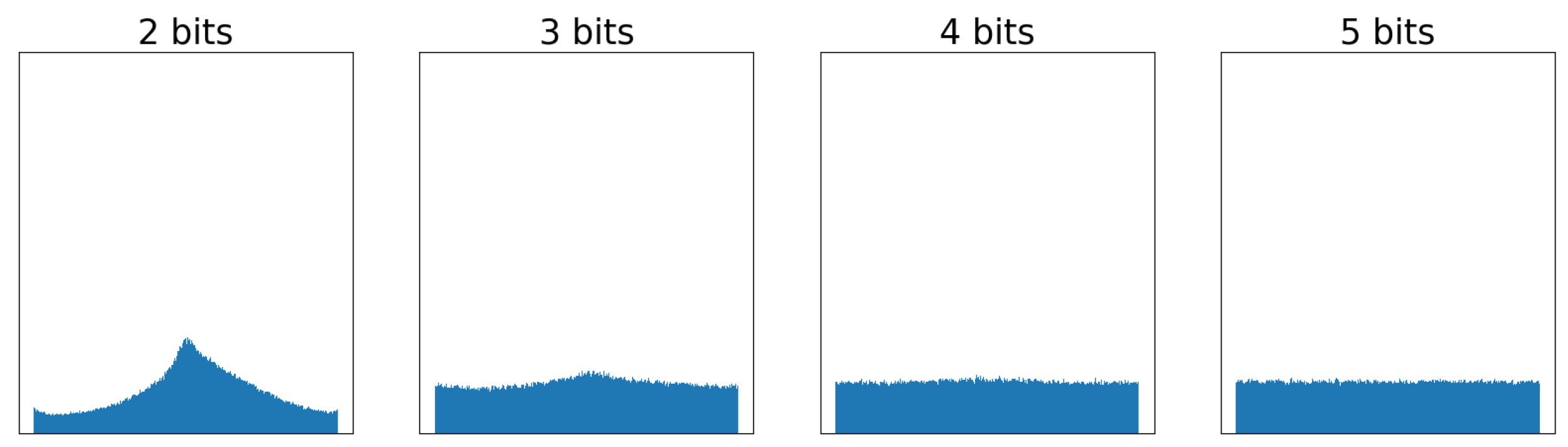
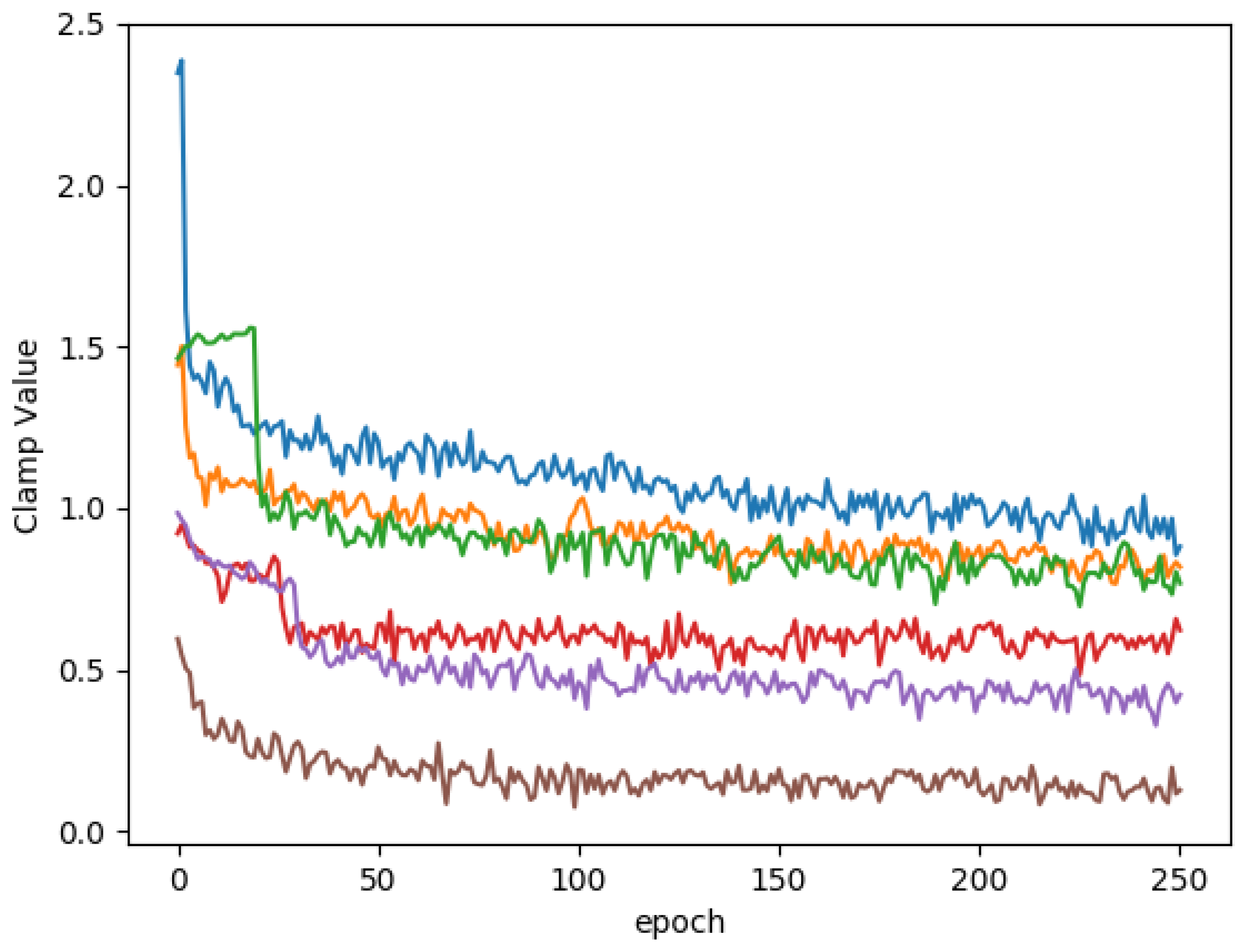
3.3. Clamping and Quantization

In order to quantize the network weights, we clamp their values in the range $[-c_w,c_w]$:

$$\begin{array}{c}\hfill w_c=Clamp(w,-c_w,c_w)=max(-c_w,min(x,c_w)).\end{array}$$

(1)

The parameter $c_w$ is defined per layer and is initialized with $c_w=\mathrm{mean}\left(w\right)+\beta \times \mathrm{std}\left(w\right)$, where w values are the weights of the layer, and $\beta$ is a hyper-parameter. Given $c_w$, we uniformly quantize the clamped weight into $B_w$ bits according to

$$\widehat{w}=\left[w_c\frac{2^{B_w-1}-1}{c_w}\right]\frac{c_w}{2^{B_w-1}-1},$$

where $[·]$ denotes the rounding operation.

The quantization of the network activations is performed in a similar manner. The conventional ReLU activation function in CNNs is replaced by the clamped ReLU,

$$\begin{array}{c}\hfill a_c=Clamp(a,0,c_a),\end{array}$$

(2)

where a denotes the output of the linear part of the layer, $a_c$ is the nonnegative value of the clamped activation prior to quantization, and $c_a$ is the clamping range. The constant $c_a$ is set as a local parameter of each layer and is learned with the other parameters of the network via backpropagation. We used the initialization $c_a=\mathrm{mean}\left(a\right)+\alpha \times \mathrm{std}\left(a\right)$ with the statistics computed on the training dataset and $\alpha$ set as a hyper-parameter.

A quantized version of the truncated activation is obtained by quantizing $a_c$ uniformly to $B_a$ bits,

$$\begin{array}{c}\hfill \widehat{a}=\left[a_c\frac{2^{B_a}-1}{c_a}\right]·\frac{c_a}{2^{B_a}-1}.\end{array}$$

(3)

Since the Round function is non-differentiable, we used the STE approach to propagate the gradients through it to the next layer. For the update of $c_a$, we calculated the derivative of $\widehat{a}$ with respect to $c_a$ as

$$\begin{array}{c}\hfill \frac{\partial \widehat{a}}{\partial a_c}=\{\begin{array}{cc}1,\hfill & a_c\in [0,c_a]\hfill \\ 0,\hfill & \mathrm{otherwise}.\hfill \end{array}\end{array}$$

(4)

Figure 2 depicts the evolution of the activation clamp values throughout the epochs. In this experiment, $\alpha$ was set to 5. It can be seen that activation clamp values converge to values smaller than the initialization. This shows that the layer prefers to shrink the dynamic range of the activations, which can be interpreted as a form of regularization similar in its purpose to weight decay on weights.

The quantization of the layer biases is more complex, since their scale depends on the scales of both the activations and the weights. For each layer, we initialize the bias clamping value as

$$c_b=(\underset{\mathrm{Activation\; scale}}{\underbrace{\frac{c_a}{2^{B_a}-1}}}·\underset{\mathrm{Weight\; scale}}{\underbrace{\frac{c_w}{2^{B_w-1}-1}}})·\left(\underset{\mathrm{Maximal\; bias\; value}}{\underbrace{2^{B_b-1}-1}}\right),$$

(5)

where $B_b$ denotes the bias bitwidth. The biases are clamped and quantized in the same manner as the weights.

4. Results

To demonstrate the effectiveness of our method, we implemented it in PyTorch and evaluated it using image classification datasets (ImageNet and CIFAR-10) and a regression scenario (the MSR joint denoising and demosaicing dataset [38]). In all the experiments, we used a pre-trained FP32 model, which was then quantized using NICE.

4.1. CIFAR-10

We tested NICE with ResNet-18 on CIFAR-10 for various quantization levels of the weights and activations.

Table 1. NICE accuracy (% top-1) on CIFAR-10 for range of bitwidths.

	Activation Bits
		1	2	3	32
Weight bits	2	89.5	92.53	92.69	92.71
	3	91.32	92.74	93.01	93.26
	32	91.87	93.04	93.15	93.02

reports the results. Notice that for the case of 3 bit weights activations, we obtain the same accuracy and for the 2 bit case, only a small degradation. Moreover, observe that when we quantize only the weights or activations, we get a nice regularization effect that improves the achieved accuracy.

4.2. ImageNet

For quantizing the ResNet-18/34/50 networks for ImageNet, we fine-tuned a given pre-trained network using NICE. We trained a network for a total of 120 epochs, following the gradual process described in Section 3.2 with the number of stages N set to the number of trainable layers. We used an SGD optimizer with a learning rate of ${10}^{-4}$, momentum of $0.9$, and weight decay of $4\times {10}^{-5}$.

Table 2. ImageNet comparison. We report top-1, top-5 accuracy on ImageNet compared with state-of-the-art prior methods. For each DNN architecture, rows are sorted in number of bits. Baseline results were taken from PyTorch model zoo. Compared methods: JOINT [28], PACT [29], LQ-Nets [18], FAQ [31].

Network	Method	Precision (w,a)	Accuracy (% Top-1)	Accuracy (% Top-5)
ResNet-18	baseline	32,32	69.76	89.08
ResNet-18	FAQ	8,8	70.02	89.32
ResNet-18	NICE (Ours)	5,5	70.35	89.8
ResNet-18	PACT	5,5	69.8	89.3
ResNet-18	NICE (Ours)	4,4	69.79	89.21
ResNet-18	JOINT	4,4	69.3	-
ResNet-18	PACT	4,4	69.2	89.0
ResNet-18	FAQ	4,4	69.81	89.10
ResNet-18	LQ-Nets	4,4	69.3	88.8
ResNet-18	JOINT	3,3	68.2	-
ResNet-18	NICE (Ours)	3,3	67.68	88.2
ResNet-18	LQ-Nets	3,3	68.2	87.9
ResNet-18	PACT	3,3	68.1	88.2
ResNet-34	baseline	32,32	73.30	91.42
ResNet-34	FAQ	8,8	73.71	91.63
ResNet-34	NICE (Ours)	5,5	73.72	91.60
ResNet-34	NICE (Ours)	4,4	73.45	91.41
ResNet-34	FAQ	4,4	73.31	91.32
ResNet-34	LQ-Nets	3,3	71.9	88.15
ResNet-34	NICE (Ours)	3,3	71.74	90.8
ResNet-50	baseline	32,32	76.15	92.87
ResNet-50	FAQ	8,8	76.52	93.09
ResNet-50	PACT	5,5	76.7	93.3
ResNet-50	NICE (Ours)	5,5	76.73	93.31
ResNet-50	NICE (Ours)	4,4	76.5	93.3
ResNet-50	LQ-Nets	4,4	75.1	92.4
ResNet-50	PACT	4,4	76.5	93.2
ResNet-50	FAQ	4,4	76.27	92.89
ResNet-50	NICE (Ours)	3,3	75.08	92.35
ResNet-50	PACT	3,3	75.3	92.6
ResNet-50	LQ-Nets	3,3	74.2	91.6

compares NICE with other leading approaches to low-precision quantization [18,28,29,31]. Various quantization levels of the weights and activations are presented. As a baseline, we used a pre-trained full-precision model.

Our approach achieves state-of-the-art results for 4 and 5 bits quantization and comparable results for 3 bits quantization, on the different network architectures. Moreover, notice that our results for the 5,5 setup, on all the tested architectures, have slightly outperformed the FAQ 8,8 results.

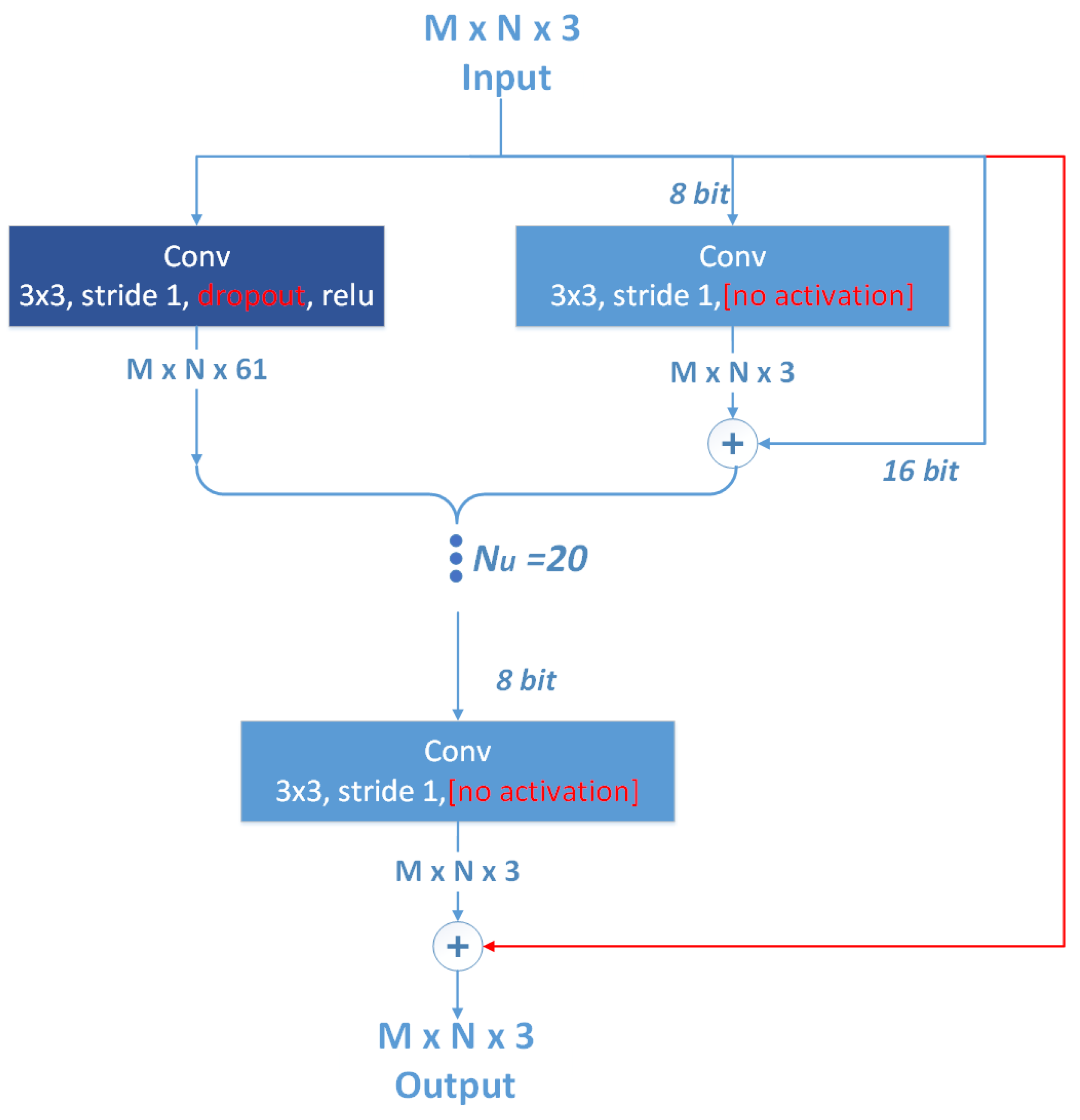
4.3. Regression—Joint Denoising and Demosaicing

In addition to the classification tasks, we apply NICE on a regression task—namely, joint image denoising and demosaicing. The network we used is the one proposed in [13]. We slightly modified it by adding to it Dropout with $p=0.05$, removing the tanh activations, and adding skip connections between the input and the output images. These skip connections improve the quantization results as, in this case, the network only needs to learn the necessary modifications to the input image. Figure 3 shows the whole network, where the modifications are marked in red. The three channels of the input image are quantized to 16 bits, while the output of each convolution, when followed by an activation, are quantized to 8 bits (marked in Figure 3). The first and last layers are also quantized.

We applied NICE on a full-precision pre-trained network for 500 epochs with Adam optimizer with learning rate of $3\times {10}^{-5}$. The data were augmented with random horizontal and vertical flipping. Since we are not aware of any other work of quantization for this task, we implemented WRPN [17] as a baseline for comparison.

Table 3. PSNR [dB] results on joint denoising and demosaicing for different bitwidths.

Method	Bits	Bits	Bits	Bits	Bits
	(w = 32, a = 32)	(w = 4, a = 8)	(w = 4, a = 6)	(w = 4, a = 5)	(w = 3, a = 6)
NICE (Ours)	39.696	39.456	39.332	39.167	38.973
WRPN (our experiments)	39.696	38.086	37.496	36.258	36.002

reports the test set PSNR for the MSR dataset [38]. It can be clearly seen that NICE achieves significantly better results than WRPN, especially for low-weight bitwidths.

4.4. Ablation Study

In order to show the importance of each part of our NICE method, we used ResNet-18 on ImageNet.

Table 4. Ablation study of NICE scheme. Accuracy (% top-1) for ResNet-18 on ImageNet for different setups.

Noise with Gradual Training	Activation Clamping Learning	Accuracy on 5,5 [w,a]	Accuracy on 3,3 [w,a]
-	-	69.72	66.51
-	✓	69.9	67.2
✓	-	70.25	66.7
✓	✓	70.3	67.68

reports the accuracy for various combinations of the NICE components. Notice that for high bitwidths, i.e., 5,5, the noise addition and gradual training contribute to the accuracy more than the clamp learning. This happens since (i) the noise distribution is indeed uniform in this case, as we show in Figure 1 and (ii) the relatively high number of activation quantization levels almost negates the effect of clamping. For low bitwidths, i.e., 3,3, we observe the opposite. The uniform noise assumption is no longer accurate. Moreover, due to the small number of bits, clamping the range of values becomes more significant.

5. Hardware Implementation

5.1. Optimizing Quantization Flow for Hardware Inference

Our quantization scheme can fit an FPGA implementation well for several reasons. Firstly, uniform quantization of both the weights and activation induces uniform steps between each quantized bin. This means that we can avoid the use of a resource costly codebook (look-up table) with the size $B_a\times B_w\times B_a$, for each layer. This also saves calculation time.

Secondly, our method enables having an integer-only arithmetic. In order to achieve that, we start, following (5), by representing each activation and network parameter in the form of $X=N\times S$, where N is the integer code and S is a pre-calculated scale. We then reformulate the scaling factors S into the form $\widehat{S}=q\times 2^p$, where $q\in \mathbb{N},p\in \mathbb{Z}$. Practically, we found that it is sufficient to constrain these values to $q\in [1,256]$ and $p\in [-32,0]$ without an accuracy drop. This representation allows the replacement of hardware costly floating-point operations by a combination of cheap shift operations and integer arithmetics.

5.2. Hardware Flow

In the hardware implementation, for both the regression and the classification tasks, we adopt the PipeCNN [39] implementation released by the authors. (https://github.com/doonny/PipeCNN access on 12 August 2021) In this implementation, the FPGA is programmed with an image containing data moving, convolution, and a pooling kernel. Layers are calculated sequentially. Figure 4 illustrates the flow of feature maps in the residual block from a previous layer to the next one. $S{a}_i,S{w}_i$ are the activations and weights scale factors of layer i, respectively. All these factors are calculated offline and are loaded to the memory along with the rest of the parameters. Note that we use the FPGA for inference only.

We compiled the OpenCL kernel to Intel’s Arria 10 FPGA and ran it with the regression architecture in Figure 3. Weights were quantized to 4 bits, activations to 8 bits, and biases, and the input image to 16 bits. The resource utilization amounts to 222 K LUTs, 650 DSP Blocks, and 35.3 Mb of on-chip RAM. With a maximum clock frequency of 240 MHz, the processing of a single image takes 250 ms. In terms of power, the FPGA requires 30 W, while an NVIDIA Titan X GPU requires 160 W. From standard hardware design practices, we can project that a dedicated ASIC manufactured using a similar process would be much more efficient by at least one order of magnitude.

6. Conclusions

We introduced NICE —a training scheme for quantized neural networks. The scheme is based on using uniform quantized parameters, additive uniform noise injection, and learning the quantization clamping range. The scheme is amenable to efficient training by backpropagation in full precision arithmetic. One advantage of NICE is the ease of its implementation on existing networks. In particular, it does not require changes in the architecture of the network, such as increasing the number of filters as required by some previous works. Moreover, NICE can be used for various types of tasks such as classification and regression.

We report state-of-the-art results on ImageNet for a range of bitwidths and network architectures. Our solution outperforms current works on both the 4,4 and 5,5 setups, for all tested architectures, including non-uniform solutions such as [18]. It shows comparable results in the 3,3 setup.

We showed that quantization error for 4 and 5 bits distributes uniformly, which explains the larger success of our method in these bitwidths compared to the case of 3 bits. This implies that the results for less than 4 bits may be further improved by adding non-uniform noise to the parameters. However, the 4 bit quantization is of special interest since, being a power of 2, it is considered more hardware friendly, and INT4 matrix multiplications are supported by Tensor Cores in recently announced inference-oriented Nvidia’s Tesla GPUs.

References

1. Hinton, G.; Deng, L.; Yu, D.; Dahl, G.E.; Mohamed, A.R.; Jaitly, N.; Senior, A.; Vanhoucke, V.; Nguyen, P.; Sainath, T.N.; et al. Deep Neural Networks for Acoustic Modeling in Speech Recognition: The Shared Views of Four Research Groups. IEEE Signal Process. Mag. 2012, 29, 82–97. [Google Scholar] [CrossRef]
2. Lai, S.; Xu, L.; Liu, K.; Zhao, J. Recurrent Convolutional Neural Networks for Text Classification. In Proceedings of the Twenty-Ninth AAAI Conference on Artificial Intelligence, AAAI’15, Austin, TX, USA, 25–30 January 2015; pp. 2267–2273. [Google Scholar]
3. Chen, L.; Papandreou, G.; Kokkinos, I.; Murphy, K.; Yuille, A.L. DeepLab: Semantic Image Segmentation with Deep Convolutional Nets, Atrous Convolution, and Fully Connected CRFs. IEEE Trans. Pattern Anal. Mach. Intell. 2018, 40, 834–848. [Google Scholar] [CrossRef] [PubMed]
4. He, K.; Zhang, X.; Ren, S.; Sun, J. Deep Residual Learning for Image Recognition. In Proceedings of the IEEE Conference on Computer Vision and Pattern Recognition (CVPR), Las Vegas, NV, USA, 27–30 June 2016. [Google Scholar]
5. He, Y.; Zhang, X.; Sun, J. Channel Pruning for Accelerating Very Deep Neural Networks. In Proceedings of the IEEE International Conference on Computer Vision (ICCV), Venice, Italy, 22–29 October 2017. [Google Scholar]
6. Molchanov, D.; Ashukha, A.; Vetrov, D. Variational Dropout Sparsifies Deep Neural Networks. In Proceedings of the International Conference on Machine Learning, Sydney, Australia, 6–11 August 2017. [Google Scholar]
7. Yu, X.; Liu, T.; Wang, X.; Tao, D. On Compressing Deep Models by Low Rank and Sparse Decomposition. In Proceedings of the IEEE Conference on Computer Vision and Pattern Recognition (CVPR), Honolulu, HI, USA, 21–26 July 2017. [Google Scholar]
8. Denton, E.; Zaremba, W.; Bruna, J.; LeCun, Y.; Fergus, R. Exploiting Linear Structure Within Convolutional Networks for Efficient Evaluation. arXiv 2014, arXiv:1404.0736. [Google Scholar]
9. Iandola, F.N.; Moskewicz, M.W.; Ashraf, K.; Han, S.; Dally, W.J.; Keutzer, K. SqueezeNet: AlexNet-level accuracy with 50x fewer parameters and <1 MB model size. arXiv 2016, arXiv:1602.07360. [Google Scholar]
10. Wu, B.; Wan, A.; Yue, X.; Jin, P.H.; Zhao, S.; Golmant, N.; Gholaminejad, A.; Gonzalez, J.; Keutzer, K. Shift: A Zero FLOP, Zero Parameter Alternative to Spatial Convolutions. arXiv 2017, arXiv:1711.08141. [Google Scholar]
11. Gupta, S.; Agrawal, A.; Gopalakrishnan, K.; Narayanan, P. Deep learning with limited numerical precision. In Proceedings of the 32nd International Conference on Machine Learning (ICML-15), Lille, France, 6–11 July 2015; pp. 1737–1746. [Google Scholar]
12. Jacob, B.; Kligys, S.; Chen, B.; Zhu, M.; Tang, M.; Howard, A.; Adam, H.; Kalenichenko, D. Quantization and Training of Neural Networks for Efficient Integer-Arithmetic-Only Inference. In Proceedings of the IEEE Conference on Computer Vision and Pattern Recognition (CVPR), Salt Lake City, UT, USA, 18–22 June 2018. [Google Scholar]
13. Schwartz, E.; Giryes, R.; Bronstein, A.M. DeepISP: Learning End-to-End Image Processing Pipeline. arXiv 2018, arXiv:1801.06724. [Google Scholar] [CrossRef] [Green Version]
14. Polino, A.; Pascanu, R.; Alistarh, D. Model compression via distillation and quantization. arXiv 2018, arXiv:1802.05668. [Google Scholar]
15. Rastegari, M.; Ordonez, V.; Redmon, J.; Farhadi, A. Xnor-net: Imagenet classification using binary convolutional neural networks. In European Conference on Computer Vision; Springer: Cham, Switzerland, 2016; pp. 525–542. [Google Scholar]
16. Hubara, I.; Courbariaux, M.; Soudry, D.; El-Yaniv, R.; Bengio, Y. Quantized Neural Networks: Training Neural Networks with Low Precision Weights and Activations. J. Mach. Learn. Res. 2018, 18, 1–30. [Google Scholar]
17. Mishra, A.; Nurvitadhi, E.; Cook, J.J.; Marr, D. WRPN: Wide Reduced-Precision Networks. arXiv 2017, arXiv:1709.01134. [Google Scholar]
18. Zhang, D.; Yang, J.; Ye, D.; Hua, G. LQ-Nets: Learned Quantization for Highly Accurate and Compact Deep Neural Networks. In Proceedings of the European Conference on Computer Vision (ECCV), Munich, Germany, 8–14 September 2018. [Google Scholar]
19. Zhu, C.; Han, S.; Mao, H.; Dally, W.J. Trained ternary quantization. arXiv 2016, arXiv:1612.01064. [Google Scholar]
20. Banner, R.; Hubara, I.; Hoffer, E.; Soudry, D. Scalable Methods for 8-bit Training of Neural Networks. arXiv 2018, arXiv:1805.11046. [Google Scholar]
21. Zhou, A.; Yao, A.; Guo, Y.; Xu, L.; Chen, Y. Incremental Network Quantization: Towards Lossless CNNs with Low-Precision Weights. In Proceedings of the International Conference on Learning Representations, ICLR2017, Toulon, France, 24–26 April 2017. [Google Scholar]
22. Hubara, I.; Courbariaux, M.; Soudry, D.; El-Yaniv, R.; Bengio, Y. Binarized neural networks. arXiv 2016, arXiv:1602.02830. [Google Scholar]
23. Zhou, S.; Wu, Y.; Ni, Z.; Zhou, X.; Wen, H.; Zou, Y. DoReFa-Net: Training low bitwidth convolutional neural networks with low bitwidth gradients. arXiv 2016, arXiv:1606.06160. [Google Scholar]
24. Cai, Z.; He, X.; Sun, J.; Vasconcelos, N. Deep Learning with Low Precision by Half-wave Gaussian Quantization. In Proceedings of the IEEE Computer Society Conference on Computer Vision and Pattern Recognition, Honolulu, HI, USA, 21–26 July 2017. [Google Scholar]
25. Bengio, Y.; Léonard, N.; Courville, A.C. Estimating or Propagating Gradients Through Stochastic Neurons for Conditional Computation. arXiv 2013, arXiv:1308.3432. [Google Scholar]
26. Hinton, G.; Vinyals, O.; Dean, J. Distilling the Knowledge in a Neural Network. arXiv 2015, arXiv:1503.02531. [Google Scholar]
27. Mishra, A.; Marr, D. Apprentice: Using Knowledge Distillation Techniques To Improve Low-Precision Network Accuracy. arXiv 2017, arXiv:1711.05852. [Google Scholar]
28. Jung, S.; Son, C.; Lee, S.; Son, J.; Kwak, Y.; Han, J.J.; Choi, C. Joint Training of Low-Precision Neural Network with Quantization Interval Parameters. arXiv 2018, arXiv:1808.05779. [Google Scholar]
29. Choi, J.; Wang, Z.; Venkataramani, S.; Chuang, P.I.; Srinivasan, V.; Gopalakrishnan, K. PACT: Parameterized Clipping Activation for Quantized Neural Networks. arXiv 2018, arXiv:1805.06085. [Google Scholar]
30. Dong, Y.; Ni, R.; Li, J.; Chen, Y.; Zhu, J.; Su, H. Learning Accurate Low-Bit Deep Neural Networks with Stochastic Quantization. In Proceedings of the British Machine Vision Conference (BMVC’17), London, UK, 4–7 September 2017. [Google Scholar]
31. McKinstry, J.L.; Esser, S.K.; Appuswamy, R.; Bablani, D.; Arthur, J.V.; Yildiz, I.B.; Modha, D.S. Discovering Low-Precision Networks Close to Full-Precision Networks for Efficient Embedded Inference. arXiv 2018, arXiv:1809.04191. [Google Scholar]
32. Arora, S.; Ge, R.; Neyshabur, B.; Zhang, Y. Stronger generalization bounds for deep nets via a compression approach. In Proceedings of the International Conference on Machine Learning (ICML), Stockholm, Sweden, 10–15 July 2018. [Google Scholar]
33. Karbachevsky, A.; Baskin, C.; Zheltonozhskii, E.; Yermolin, Y.; Gabbay, F.; Bronstein, A.M.; Mendelson, A. Early-Stage Neural Network Hardware Performance Analysis. Sustainability 2021, 13, 717. [Google Scholar] [CrossRef]
34. Baskin, C.; Schwartz, E.; Zheltonozhskii, E.; Liss, N.; Giryes, R.; Bronstein, A.M.; Mendelson, A. UNIQ: Uniform Noise Injection for the Quantization of Neural Networks. arXiv 2018, arXiv:1804.10969. [Google Scholar]
35. Sripad, A.; Snyder, D. A necessary and sufficient condition for quantization errors to be uniform and white. IEEE Trans. Acoust. Speech, Signal Process. 1977, 25, 442–448. [Google Scholar] [CrossRef]
36. Gray, R.M. Quantization noise spectra. IEEE Trans. Inf. Theory 1990, 36, 1220–1244. [Google Scholar] [CrossRef]
37. Xu, C.; Yao, J.; Lin, Z.; Ou, W.; Cao, Y.; Wang, Z.; Zha, H. Alternating Multi-bit Quantization for Recurrent Neural Networks. arXiv 2018, arXiv:1802.00150. [Google Scholar]
38. Khashabi, D.; Nowozin, S.; Jancsary, J.; Fitzgibbon, A.W. Joint Demosaicing and Denoising via Learned Nonparametric Random Fields. IEEE Trans. Image Process. 2014, 23, 4968–4981. [Google Scholar] [CrossRef]
39. Wang, D.; An, J.; Xu, K. PipeCNN: An OpenCL-Based FPGA Accelerator for Large-Scale Convolution Neuron Networks. arXiv 2016, arXiv:1611.02450. [Google Scholar]
Figure 1. Weight quantization error histogram for a range of bitwidths.
Mathematics 09 02144 g001
Figure 2. Activation clamp values during ResNet-18 training on CIFAR10 dataset.
Mathematics 09 02144 g002
Figure 3. Model used in denoising/demosaicing experiment.
Mathematics 09 02144 g003
Figure 4. Residual block in hardware.
Mathematics 09 02144 g004